Information-Theoretic Measures and Modeling Stock Market Volatility: A Comparative Approach

Abstract

The volatility analysis of stock returns data is paramount in financial studies. We investigate the dynamics of volatility and randomness of the Pakistan Stock Exchange (PSX-100) and obtain insights into the behavior of investors during and before the coronavirus disease (COVID-19 pandemic). The paper aims to present the volatility estimations and quantification of the randomness of PSX-100. The methodology includes two approaches: (i) the implementation of EGARCH, GJR-GARCH, and TGARCH models to estimate the volatilities; and (ii) analysis of randomness in volatilities series, return series, and PSX-100 closing prices for pre-pandemic and pandemic period by using Shannon’s, Tsallis, approximate and sample entropies. Volatility modeling suggests the existence of the leverage effect in both the underlying periods of study. The results obtained using GARCH modeling reveal that the stock market volatility has increased during the pandemic period. However, information-theoretic results based on Shannon and Tsallis entropies do not suggest notable variation in the estimated volatilities series and closing prices. We have examined regularity and randomness based on the approximate entropy and sample entropy. We have noticed both entropies are extremely sensitive to choices of the parameters.

1. Introduction

Measuring and managing financial risk represent key concerns of an investor. The uncertainty of future returns from an investment involves the existence of the risk factor. The commonly used measure of risk is called the standard deviation of the return, usually known as volatility. Therefore, volatility can be regarded as a technical term in finance, and it is related directly to notions used in the asset pricing theory in finance. Measuring volatility requires time to manifest itself. Therefore, we may need to choose between various statistical estimators. The strengths and weaknesses of each method of estimation vary depending upon the choice of the model. This paper explores the performance of several volatility estimators for the Pakistan Stock Exchange, abbreviated as PSX. The PSX (formally Karachi Stock Exchange (KSE))-100 share index emerged as the integration of three local stock exchanges under the promulgation of the new Securities Act, 2015. PSX-100 has shown a significant rise and reached historic levels after the unification. In 2016, PSX-100 was declared an emerging Asian market. Pakistan’s qualification for the Morgan Stanley Capital International (MSCI) Emerging market index in 2017 resulted in a record high of 49,876 base points, which is unbroken to this day. Pakistan Stock Exchange had been named Asia’s best performer in 2016. In 2020, A New York-based global markets research firm, marketcurrentswealthnet.com (accessed on 27 April 2021), published that PSX has become the best performer in Asia and the world’s fourth-best performing market. Pakistan’s stock market is a very sensitive and highly volatile market. It reacts quickly to political news, government policies and media developed stories. On the other hand, rapid growth after unexpected returns is the typical behavior of the market. The dynamics of price movement in a stock market depends on different factors, such as monetary policy, the impact of interest rates, and the promulgation of unfavorable news. The term leverage effect used in financial literature describes the degree of stock volatility and its relationship with any sudden new information. Research on the volatility of stock market returns has always been the focus of financial economists. Therefore, it plays a crucial role to develop a link between macroeconomic policies and financial stability. In finance, volatility interprets market risk, and its prediction is vital for empirical asset pricing, risk management, and portfolio selection.

In literature, researchers have used various volatility forecasting models. These models can be classified into different categories. Some examples of these models include historical volatility models based on the computation of the standard deviation of the historical return series, the random walk model, the historical average model, the simple moving average model, exponential smoothing, and the exponentially weighted moving average model. On the other hand, some examples of the regime-switching models accommodate the threshold-autoregressive model by Cao and Tsay (1992) and the smooth transition exponential smoothing model by Taylor (2004). Few examples of research work that used historical volatility models include Taylor (1986, 1987); Figlewski (1997); Figlewski and Green (1999) and Andersen et al. (2001). In literature, these models have shown good forecasting performance as compared to other class of volatility models. Poon and Granger (2005) discussed several practical problems involved in forecasting volatility.

Engle (1982) introduced the autoregressive conditional heteroskedasticity (ARCH) model to forecast the volatility. Later, its generalized version, GARCH, was developed by Bollerslev (1986). An ARCH model describes a volatile variance over time and incorporates all past error terms. The model is effective for any series that has increased or decreased variance. For the higher-order ARCH process, it is more convenient to use the GARCH model. In this model, the conditional variance is a linear function of its lags. GARCH models provide insight into the nature, extent, and implication of volatility for stock market volatility. The GARCH models have been rapidly extended, and a large family of these models exists in the literature. The standard GARCH models assume symmetric effects on volatility. It leads to the shortfall of these models, that good and bad news has a similar impact on volatility. The standard GARCH model assumes normality condition for errors. As a result, they generally fail to account for excessive skewness and kurtosis in stock returns. In literature, there are thousands of papers on GARCH modeling. Hence, we cannot list all. Therefore, we include a few famous models. The exponential GARCH (EGARCH) model proposed by Nelson (1991) is used to capture serial dependence and leverage effects. GJR-GARCH process of Glosten et al. (1993) models positive and negative shocks on the conditional variance asymmetrically using the indicator function. Asymmetric power ARCH (APARCH) proposed by Ding et al. (1993) is efficient in capturing the conditional-heteroscedasticity behavior in volatility. Zakoian (1994) proposed the threshold GARCH (TGARCH) model. This model is frequently used to handle the leverage effects of good news and bad news on volatility. Lee and Engle (1999) proposed a component-GARCH or CGARCH model to investigate the long and short-run estimates of volatility. McMillan et al. (2000) used threshold GARCH (TGARCH) and EGARCH models for the volatility forecast of daily, weekly, and monthly period for the United Kingdom (UK) Financial Times Actuaries (FTA). Ng and McAleer (2004) compared TARCH and standard GARCH models to forecast the volatility of the daily returns of the Standard and Poor (S&P) 500 Composite Index and the Nikkei 225 Index.

The volatility performance of models that exhibit the asymmetric effect is critical in financial studies. For example, Patev and Kanaryan (2008) applied several asymmetric and symmetric GARCH models on the central European stock market. Similarly, Harrison and Moor (2012) forecasted the stock market volatility of 10 stock exchanges in emerging Central and Eastern European (CEE) countries using asymmetric GARCH models. Abdalla and Suliman (2012) implemented the GARCH models to the Saudi stock market, including a symmetric and asymmetric version. Okicic (2015) investigated the existence of the leverage effect in stock markets of the CEE region. Additionally, in recent studies, we can find systematic reviews on GARCH models and applications. For example, Dhanaiah and Prasad (2017) studied the literature on volatility and co-movements models. In addition, Hussain et al. (2019) have reviewed the empirical literature on stock market volatility. A systematic review of GARCH models to forecast the stock returns volatility was recently given by Bhowmik and Wang (2020).

In information theory, entropy represents a concept used to evaluate the uncertainty or self-information of a source. The use of information measures has now become an alternative method of solving various problems in finance. For example, researchers have used the concept of entropy to measure the variations in the price returns, volatility modeling, option pricing, portfolio selection, and asset pricing. The use of information measures is another way of finding the non-linear dynamics of volatility. Entropy was first defined by German physicist Rudolph Clausius in the mid-nineteenth century. Later, Shannon (1948) introduced information entropy to deal with the entropy of a random variable. It measures the amount of information supplied by a probabilistic experiment or a random variable, based on Boltzmann’s entropy (Boltzmann 1896) from statistical physics. The Shannon entropy can be used in particular manners to evaluate the entropy corresponding to a probability density distribution around some points. Alternatively, sometimes specific events of interest are significantly important. For example, the deviation from the mean, a piece of sudden news, affecting the stock market. At this point, the generalization of the classical concept of entropy is vital. Rényi (1961) introduced an entropy measure. Rényi measure depends on the power of the probability law. Tsallis (1988) proposed a new entropy measure that successfully describes the statistical features of complex systems. Pincus (1991) introduced approximate entropy (ApEn). It is an index of complexity and uncertainty for a given time series. Sample entropy (SampEn), a modification of ApEn, was proposed by Richman and Moorman (2000). The SampEn measures the complexity of the physiological time series. Bentes and Menezes (2012) used information measures to investigate the stock market volatility. Sheraz et al. (2015) assessed volatile stock markets using entropy measures, including the Shannon, Tsallis, Rényi, and approximate entropy. Pele et al. (2017) studied measures of market risk by using an information entropic approach. Gençay and Gradojevic (2017) discussed a comparative analysis of the stock market dynamics based on entropy. Lahmiri and Bekiros (2020a) applied informational entropy methods to evaluate the impact of the COVID-19 pandemic on randomness in the volatility of the major world stock markets. Many different entropic methods have been proposed to study the financial markets, for example, Gulko (1999); Gençay and Gradojevic (2008, 2010); Zhou et al. (2013); Preda et al. (2014); Toma (2014); Preda and Sheraz (2015) and Sheraz et al. (2019).

After the outbreak of the COVID-19 pandemic, several studies have listed in the literature on the performance of the financial markets, such as the stock market volatility. The infectious disease affected the functioning of companies and changes in human mobility, which also indirectly affects the situation on the stock exchanges. For example, Zimon and Tarighi (2021) investigated the impacts of the COVID-19 pandemic on working capital management policies among small and medium-sized enterprises. Aruga (2021) studied the effect of the caused changes in human mobility due to the announcement of the state of emergency to cope with the COVID-19 pandemic on the Tokyo gasoline, diesel, and kerosene markets.

Multiple studies predicted the global stock markets performances during the pandemic period. Topcu and Gulal (2020) investigated the pandemic impact on emerging stock markets of Asia is higher than that of the European markets. Libo Xu (2021) studied Canadian and US stock markets to explore the unexpected changes and uncertainty of markets. Liu et al. (2021) investigated the impact of the pandemic on the Chinese stock market crash risk by using the approach of GARCH processes. Szczygielski et al. (2021) examined the effect of COVID-19 uncertainty on Asia and found that it exceeds, Europe, Africa, Latin America, North America, and Arab markets indices returns.

The literature on the volatility dynamics of PSX-100 is, however, limited. Recently, Ali et al. (2020) studied the relationship of PSX-100 volatility, exchange rate, and gold prices for two divided periods of 2001–2008 and 2008–2018. Waheed et al. (2020) proposed that the Pakistani market showed confirmed positive increments in stock returns during the pandemic. Alamgir and Amin (2021) examine the link between oil prices and stock market volatility of selected South-Asian countries. To our best knowledge, no studies have been conducted on the volatility dynamics of PSX-100 using the information-theoretic measures and comparisons with traditional methods. We aim to fill the existing research gap on the most emerging and best performer market of Asia. Given the preceding discussion and arguments, we set the following hypothesis.

Hypothesis 1 (H1).

The volatility market of PSX-100 has increased during the pandemic period with the notable existence of the leverage effect in the case of GARCH modeling.

To investigate H1, we divide our data into two periods: (i) COVID-19 pandemic, (ii) Before COVID-19 pandemic, and employed three asymmetric GARCH models.

Hypothesis 2 (H2).

The randomness and regularity of PSX-100 closing prices, returns and estimated volatility series are higher during the COVID-19 pandemic period.

To investigate H2, following the aforementioned periods we implement Shannon, Tsallis, approximate and sample entropies.

PSX-100 is a very sensitive and highly volatile market. It reacts quickly to political news, government policies and media developed stories. As we mentioned earlier, PSX-100 performance was counted best, and the goal of the study is to check the behavior of the market in a sample of the same size considered for the pandemic period. In addition, the year 2019 was understandably smooth as compared to the COVID-year 2020. Therefore, our primary goal is to compare the performance of the market in a medium-sized sample that is equal in size to the sample taken during the pandemic.

This paper discusses the volatility dynamics of PSX-100 returns. We perform GARCH modeling to estimate the volatility series of the pre-pandemic period and COVID-19 pandemic period. Information-theoretic approaches have been used to understand the randomness, regularity, and persistence of the estimated volatilities, closing prices, and closing return series. The methodology section of the paper represents the mathematical framework used for empirical results. In Section 3, we present a detailed empirical analysis of volatility estimation, randomness, and regularity. These results are based on two distinct approaches: (i) asymmetric GARCH models and (ii) entropy measures. The last section concludes the paper.

2. Methodology

2.1. Volatility

Modeling and forecasting the volatility of the stock prices is critical in risk management and financial studies. Let $R_t$ denotes the returns of the underlying stock market at time t.

$$R_t=\ln \frac{x_t}{x_{t-1}}$$

(1)

where ${\left\{X_t\right\}}_{t \in T}$ represents the stock price process. Statistically, volatility is often computed as the sample standard deviation given by

$$S=\sqrt{\frac{1}{T-1}{{\displaystyle \sum }}_{t-1}^T{\left(R_t-\mu \right)}^2}$$

(2)

where $\mu$ is the average return over the period T. The historical volatility of the annual logarithmic returns is customarily denoted by $\sigma$ and computed by the following equation:

$$\sigma =S\sqrt{\Delta t}$$

(3)

where t denotes annual 252 trading days, usually. The estimated historical volatility $\sigma$ captures only linear relationships and assumes all events are equally weighted.

2.2. GARCH Models

One of the crucial characteristics of financial market volatility is the time-varying nature of asset returns fluctuations. Engle (1982) developed the autoregressive conditional heteroskedasticity (ARCH). It was later modified to GARCH by Bollerslev (1986). Generalized autoregressive conditionally heteroscedastic models, abbreviated as GARCH, are the most popular and flexible to capture the volatility clustering. In this paper, we have used EGARCH, TGARCH, and the GJR-GARCH models. We estimate and predict the volatility series of open, high, low, and closing returns series before and during the pandemic period. The standard sGARCH model has the following mathematical form:

$$R_t={\mu }_t+{\epsilon }_t$$

(4)

$${\epsilon }_t=Z_t{\sigma }_t,Z_t ~ N\left(0,1\right)$$

(5)

$${\sigma }_t^2=\omega +{{\displaystyle \sum }}_{i=1}^p{\alpha }_i{\epsilon }_{t-1}^2+{{\displaystyle \sum }}_{j=1}^q{\beta }_j{\sigma }_{t-j}^2 \mathrm{for} t\in \mathbb{Z}$$

(6)

• The process ${\left\{{\epsilon }_t\right\}}_{t\in \mathbb{Z}}$ is called GARCH (p, q) process if $E\left({\epsilon }_t|{ℱ}_{t-1}\right)=0,$ and $Var\left({\epsilon }_t|{ℱ}_{t-1}\right)={\sigma }_t^2$;
• The random variables $Z_t$ are identical and independent, ${\epsilon }_t$ is the residual series and ${\sigma }_t^2$ its conditional variance;
• $\omega >0,{\alpha }_i\ge 0$, ${\beta }_j\ge 0$ are real parameters and ensures that ${\sigma }_t^2>0$ at all times.

In financial time series, the leverage effect predicts that an asset’s returns may become more volatile when its price decreases. Nelson (1991) proposed EGARCH processes to model the leverage effect. The EGARCH (1,1) model is given by:

$$\log \left({\sigma }_t^2\right)=\omega +{\alpha }_1 \left(\left|Z_{t-1}\right|-\mathbb{E}\left(\left|Z_{t-1}\right|\right)\right)+{\beta }_1\log \left({\sigma }_{t-1}^2\right)+{\gamma }_1{Z}_{t-1}$$

(7)

• where$\delta >0,{\alpha }_1\ge 0, {\beta }_1\ge 0, \left|{\gamma }_1\right|<1,$ and$\omega >0$. ${\alpha }_1$ and ${\gamma }_1$ represent sign effect and leverage effect;
• For leverage effect ${\gamma }_1$ must be statistically significant and negative;
• Returns are stationary if $0<{\beta }_1<1$ and EGARCH captures serial dependence and leverage effects in returns;
• If $\left|Z_{t-1}\right|$ is small, then ${\sigma }_t$ decreases. For large $\left|Z_{t-1}\right|$ , the value of ${\sigma }_t$ increases;
• Due to log-transformation of variance, it guarantees positivity of variance without any restriction on parameters.

The Glosten-Jagannathan-Runkle (GJR)-GARCH due to Glosten et al. (1993), models positive and negative shocks on the conditional variance asymmetrically. The model is used to capture the negative correlation between returns and volatility. Additionally, it captures the asymmetric leverage effect. The model may be written as a special case of asymmetric power ARCH or APARCH. The GJR-GARCH (1,1) model is given by:

$${\sigma }_t^2=\omega +({\alpha }_1+{\gamma }_1{I}_{t-1}){\epsilon }_{t-1}^2+{\beta }_1{\sigma }_{t-1}^2$$

(8)

• where ${\alpha }_1>0, {\beta }_1>0,{\gamma }_1>0, \omega >0$ and${\gamma }_1$indicates asymmetry of returns;
• $I_{t-1}$ assumes value equals to 1 for ${\epsilon }_{t-1}^2<0$ (negative-shock), and zero otherwise;
• For positive and significant ${\gamma }_1$, leverage effect exists.

The threshold GARCH or TGARCH model proposed by Zakoian (1994) introduces the asymmetry by specifying the conditional variance as a function of positive and negative parts of the past innovations. The model explains the threshold effect into the volatility. A TGARCH (1,1) model is given by:

$${\sigma }_t^2=\omega +({\alpha }_1+{\gamma }_1{I}_{t-1}){\epsilon }_{t-1}^2+{\beta }_1{\sigma }_{t-1}^2$$

(9)

• where ${\alpha }_{1,+}\ge 0, {\alpha }_{1,-}\ge 0, {\beta }_1\ge 0,\mathrm{and} \omega >0$ are real parameters;
• The variable ${\sigma }_t$ is strictly positive and denotes the conditional standard deviation of ${\epsilon }_t$;
• The current volatility depends on both the modulus and the sign of the past returns through ${\alpha }_{1,+}$ and ${\alpha }_{1,-}$;
• For ${\alpha }_{1,+}>$0, the effect of the bad news is greater than those of the good news;
• The GJR-GARCH model due to Glosten et al. (1993) is a version of TGARCH, which corresponds to squaring the variables involved in Equation (8).

The parameters estimation of GARCH processes has followed the maximum likelihood estimation methods. In the standard GARCH model, the $Z_t$ series follows the standard normal distribution. However, financial times exhibits fat-tailed and leptokurtic behavior. Therefore, GARCH models have been developed under the assumption of several non-Gaussian conditional distributions of ${\epsilon }_t.$ Various goodness-of-fit criteria are used to find the best-fit model selection. Multiple penalized criteria assess the quality of the model while incorporating samples size bias and complexity of the model at the same time. We consider loglikelihood, Akaike (AIC), Bayesian (BIC), Shibata (SIC), and Hannan-Quinn (HQIC). For more details on methods of estimation of GARCH processes, model selection and applications, see Francq and Zakoian (2010).

Conditional Distributions and GARCH Modeling

Any distribution can be characterized using several features such as mean, variance, skewness, and kurtosis. Since the introduction of the heavy-tail model by Mandelbrot (1963), researchers have explored these models for stock returns provides the best results. Therefore, a choice of best-fitted distribution is vital for modeling returns and corresponding risk assessment. We choose the Student’s t-distribution proposed by Gosset’s (1908), skewed Student’s t-distribution (SST) by Hansen (1994), and generalized error distribution (GED). The GARCH model with conditional t-distribution was firstly proposed by Bollerslev (1987) to accommodate the excess kurtosis. The density function of the distribution is given by:

$$f_X\left(x;\mu ,\lambda ,\upsilon \right)=\frac{\mathsf{\Gamma }\left(\frac{\left(\upsilon +1\right)}{2}\right)}{\mathsf{\Gamma }\left(\frac{\upsilon }{2}\right)\sqrt{\lambda \upsilon \pi }}{\left[1+\frac{{\left(x-\mu \right)}^2}{\lambda \upsilon }\right]}^{-\frac{1+\upsilon }{2}}$$

(10)

• where$x\in \left[-\infty ,\infty \right],$and $\mu ,\lambda ,\upsilon$ are location, scale, and shape parameters, respectively, and $\mathsf{\Gamma }$ is a Gamma function.

The use of generalized error distribution (GED) was introduced by Nelson (1991) to capture the fat-tailed returns. The GED is a 3-parameter distribution, and it belongs to the exponential family. The density function of the distribution is equal to:

$$f_X\left(x;\mu ,\lambda ,\upsilon \right)=\frac{\upsilon \exp \left({\left|\frac{x-\mu }{\lambda }\right|}^{\upsilon }\right)}{2^{\left(1+\frac{1}{\upsilon }\right)}\lambda \mathsf{\Gamma }\left({\upsilon }^{-1}\right)}$$

(11)

• where $\mu \in \left(-\infty ,\infty \right), \lambda \in \left(0,\infty \right)$ are location and scale parameters, respectively, and $\upsilon$ represents the tail-thickness parameter;
• For $\upsilon =2$ the distribution converges to the standard normal distribution, and for $\upsilon <2$, it has thicker tails than the normal distribution.

The skewed-GED distribution abbreviated as SGED exhibits skewness. The probability density function of SGED is given by:

$$f_X\left(x;\mu ,\sigma ,\lambda ,\upsilon \right)=\frac{\upsilon \exp \left(\frac{-1}{\upsilon }{\left|\frac{x-\mu +k}{\nu \sigma \left(1+\lambda \mathrm{sign}\left(x-\mu +k\right)\right)}\right|}^{\upsilon }\right)}{2\sigma \upsilon \mathsf{\Gamma }\left({\upsilon }^{-1}\right)}$$

(12)

• where $\lambda , \upsilon$ denoted skewness and shape parameters, respectively. For negative skewness $\lambda <0$, and for positive skewness $\lambda >0$. The parameter $\lambda \in \left[-1,1\right]$;
• For $\lambda =0,$the skewed-GED distribution converges to the GED;
• The sign function equals to −1 for negative values of its argument and equals to 1 for positive values;
• The values of $k=\frac{2^{\frac{2}{\upsilon }}\sigma m\lambda \mathsf{\Gamma }\left(0.5+{\nu }^{-1}\right)}{\sqrt{\pi }}$ , and $m=\frac{\pi \left(1+3{\lambda }^2\right)\mathsf{\Gamma }\left(\frac{3}{\upsilon }\right)-{16}^{\frac{1}{\upsilon }}{\lambda }^2\mathsf{\Gamma }\left(0.5+{\nu }^{-1}\right)\mathsf{\Gamma }\left(\frac{1}{\upsilon }\right)}{\pi \mathsf{\Gamma }\left(\frac{1}{\upsilon }\right)}$

For more details on GARCH processes and SGED, see Wiśniewska and Wyłomańska (2017).

Lambert and Laurent (2001) introduced the use of standardized skewed Student’s t-distribution. The density function of the distribution is given by:

$$f_X\left(x;\xi ,\upsilon \right)=\{\begin{array}{c}\frac{2\xi }{{\xi }^2}\sigma g\left(\xi \left(\sigma x+\mu \right) ;\upsilon \right) \mathrm{if} x<\frac{\mu }{\sigma }\\ \frac{2\xi }{{\xi }^2}\sigma g\left(\frac{\sigma x+\mu }{\xi } ;\upsilon \right) \mathrm{if} x>\frac{\mu }{\sigma }\end{array}$$

(13)

• where $\xi$ denotes the asymmetry coefficient, $\mu ,\sigma$ are mean and the standard deviation, respectively.
• The density is skewed to the right if $\log \left(\xi \right)>0$ and skewed to the left if $\log \left(\xi \right)<0$.

The above three density functions have been significantly used in financial literature to model the risk and stock returns. See, for example, Lambert and Laurent (2001); Bali and Theodossiou (2006); Fan et al. (2008); Chkili et al. (2012); Zhu and Galbraith (2011); Mabrouk and Saadi (2012).

2.3. Information Theoretic Measures and Volatility Modeling

2.3.1. Shannon Entropy Measure

Shannon (1948) defined a measure of information contained by an experiment in the context of the mathematical theory of communication. The entropy measure has applications in physics, biology, economics, sociology, and other fields. In financial studies stocks, Shannon entropy measures the randomness and diversity of the price’s series. Mathematically, Shannon’s entropy gives the measure of information as a function of probabilities of occurrence of different random events. We use the concept of entropy measures to study the randomness and non-linear dynamics of the stock market volatility. The Shannon entropy of the random variable having the discrete probability distribution is defined by:

$$S\left(X\right)=-{{\displaystyle \sum }}_{i=1}^m{p}_i\ln p_i$$

(14)

• where, $X=\left(x_1,x_2,\dots ,x_m\right)$ the convention $0\ln 0=0$ holds, and $p=\left(p_1,p_2,\dots ,p_m\right)$, $p_i$ represents the probability of $x_i$ , for $i=1,2,\dots ,m$. therefore,$p_i>0$ $\forall i$ and ${{\displaystyle \sum }}_{i=1}^m{p}_i=1.$
• The entropy reaches to its maximum value if all events follow the equally likely assumption;
• The entropy corresponding to an event with probability less than one has a positive sign.

In the first step, for the Shannon entropy measure, we use the following estimation methods to assess our results.

(1)

Maximum Likelihood (ML);

(2)

effreys: Bayesian estimate with a = 1/2;

(3)

Laplace: Bayesian estimate with a = 1;

(4)

Schurmann–Grassberger (SG): Bayesian estimate with a = 1/(length of underlying asset prices series);

(5)

Minimax with a = sqrt (sum (underlying asset prices series))/(length of underlying asset prices series);

(6)

Shrink entropy: Uses James–Stein-type shrinkage at the level of cell frequencies.

The Shannon entropy can be used in particular manners to evaluate the entropy of probability distribution around some points but, in the case of special events, for example, deviation from mean and any sudden news for stock returns going up (down), additional information is needed. Therefore, the concept of Shannon entropy can be generalized. Based on Shannon entropy, many other extensions have been developed for accurate estimation. For example, Rényi, Tsallis, approximate, sample, and dispersion entropies.

2.3.2. Tsallis Entropy

Tsallis (1988) introduced a non-extensive entropy. The Shannon entropy recovers as q$\to$1, where q is the parameter of the Tsallis entropy. Tsallis entropy denoted by $T\left(X\right)$ is defined as:

$$T\left(X\right)=\frac{1-{\sum }_{i=1}^m{p}_i^q}{q-1}$$

(15)

• where$X=\left(x_1,x_2,\dots ,x_m\right),$ $0<q<\infty$ and $q\ne 1.$ Rare events of interests denote $q<1$ , and frequently encountered have $q>1$;
• The q-exponential function $e_q^x={\left(1+\left(1-q\right)x\right)}^{\frac{1}{1-q}}$ , whose inverse is the q-logarithmic function ${\ln }_q^x=\frac{x^{1-q}-1}{1-q}, q\ne 1$;
• Gell-Mann and Tsallis (2004) suggested q$\approx$1.4 for high-frequency financial returns;
• The value of the parameter q decreases to 1 as the frequency of the data decreases. The values$1\le q\le 2$ emphasize highly volatile signals.

2.3.3. Approximate and Sample Entropy

Pincus (1991) introduced approximate entropy (ApEn), derived from Kolmogorov entropy (Kolmogorov 1958). ApEn is used to compare the uncertainty of a given time series. Therefore, for a financial time series, ApEn inquires the amount of regularity and unpredictability of fluctuations. The large value of ApEn indicates more prominent uncertainty. To calculate ApEn following steps are required.

• Suppose the underlying time series, $X=\left(x_1,x_2,\dots ,x_L\right)$ of length $L$;
• For $l<L$, let $a_l\left(i\right)$ and $b_l\left(j\right)$ be two vectors of length $l$ and $d\left(a_l\left(i\right),b_l\left(j\right)\right)$ denotes distance between the two vectors. Therefore,

  $$d\left(a_l\left(i\right),b_l\left(j\right)\right)=\max \left\{\left|x_{i+k}-x_{j+k}\right|:0\le k\le l-1\right\}.$$

  (16)
• Two vectors $a_l\left(i\right)$ and $b_l\left(j\right)$ are called similar if $d\le r$, where $r>0$ denotes the specified tolerance. Now compute the relative frequency $f_i\left(r\right),$ for each of the $L-\left(l-1\right)$.

  $$f_i\left(r\right)=\frac{s_l\left(i\right)}{L-\left(l-1\right)}$$

  (17)
• where $s_l\left(i\right)$ denote number of vectors $b_l\left(j\right)$ similar to $a_l\left(i\right)$ for a fixed $i$and $l.$ Now computing the average frequency ${\eta }_l\left(r\right),$

  $${\eta }_l\left(r\right)=\frac{{\sum }_{i}ln{f}_i\left(r\right)}{L-\left(l-1\right)}$$

  (18)
• Finally, ApEn can be computed by using the following statistics.

  $${\mathrm{ApEn}}_l\left(r, L\right)={\eta }_l\left(r\right)-{\eta }_{\left(l+1\right)}\left(r\right)$$

  (19)

Richman and Moorman (2000) proposed Sample entropy (SampEn), a modification of ApEn to overcome its disadvantages. The ApEn strongly depends on the length of the data. Alternatively, the SampEn assumes the same parameters $l$ and $r$, defined for the ApEn. The SampEn is given by:

$$\mathrm{SampEn}=\ln \frac{E_1}{E_2}$$

(20)

• where$E_1$ denotes number of vectors pairs of length $l+1$ and $d\left[\left(X_l\left(i\right),X_l\left(j\right)\right)\le r\right]$ with $i\ne j$;
• $E_2$ denotes total number of templates equals to length $l$ with $i\ne j.$

Many researchers have implemented entropic approaches to study the financial time series. The use of laws of physics in economics has generated a new direction of research named econophysics. In this context, interactions in financial markets are highly non-linear, long-ranged, and unstable. Darbellay and Wuertz (2000) studied the dependence of the financial time-series using entropy measures. Properties and applications of entropy in finance are well established. For more details, see Pincus (2008); Preda and Balcau (2010); Bartiromo (2010); Tapiero (2013); Mensi (2013); Ong (2015); Pele et al. (2017); Ahn et al. (2019); Lahmiri and Bekiros (2020b); Liu et al. (2021); and Ribeiro et al. (2021).

3. Empirical Analysis

In this section, we investigate the estimation and prediction of volatility employing traditional GARCH models. We implement EGARCH, GJR-GARCH, and TGARCH models to study the leverage effect, the impact of good and bad news on the volatility series of underlying data sets. Further, we implement information-theoretic measures to examine the randomness and uncertainty of the estimated volatility series. For this purpose, we compute the Shannon entropy of the estimated volatility series with seven different estimators. Subsequently, we use the Tsallis entropy, approximate entropy, and sample entropy to assess the diversity and non-linear dynamics of the volatility series of PSX-100. We use logarithmic returns of the Pakistan Stock Exchange abbreviated as PSX-100. The logarithmic returns of all the underlying data series have been calculated by following Equation (1). The data used in our empirical analysis consists of two periods. The pre-pandemic period spans from 1 January 2019 to 31 December 2019. The second period of during-pandemic spans from 1 January 2020 to 24 December 2020. We select the daily open, high, low, and closing prices for both periods. We obtained our data from the Thomas Reuters’ data stream.

Descriptive statistics provided in

Table 1. Descriptive Statistics of PSX-100 for two periods: Before COVID-19 and COVID-19 pandemic.

Returns	Before COVID-19				COVID-19
	Closing	Opening	High	Low	Closing	Opening	High	Low
Minimum	−0.0268	−0.0268	−0.0335	−0.0367	−0.071	−0.071	−0.0666	−0.0655
1st Quartile	−0.0071	−0.0078	−0.0068	−0.0065	−0.0054	−0.0054	−0.0064	−0.0054
Median	0.0001	0.0004	0.0001	0.0012	0.0012	0.0012	0.0011	0.0022
Mean	0.0003	0.0004	0.0003	0.0004	0.0002	0.0002	0.0002	0.0002
3rd Quartile	0.0075	0.0079	0.007	0.0075	0.0085	0.0086	0.0075	0.0082
Maximum	0.0351	0.0427	0.0337	0.0374	0.0468	0.0468	0.056	0.0498
Skewness	0.1326	0.1736	0.1744	−0.0276	−1.151	−1.1479	−0.9461	−1.1668
Kurtosis	3.1178	3.206	3.3096	3.4331	8.0603	8.0203	9.1404	7.7247
SD	0.0116	0.0122	0.0107	0.0118	0.0155	0.0156	0.0138	0.0152
CV	0.0243	0.0327	0.0282	0.0323	0.0125	0.0147	0.0144	0.015
Range	0.0619	0.0696	0.0672	0.0741	0.1179	0.1179	0.1226	0.1153
Inter−Quartile range	0.0145	0.0157	0.0138	0.0141	0.0139	0.014	0.0139	0.0136
JB Stats	0.7971	1.5441	2.0296	1.6715	303.1570	298.9304	404.2784	272.5008
Lilliefors Stats	0.0479	0.0336	0.0298	0.0375	0.1281	0.1276	0.0986	0.1193
Pearson Chi Sq. Test	19.8455	10.5772	13.3577	17.6829	66.4959	66.1870	43.9431	70.3577

show high kurtosis of PSX-100 returns for the period during-pandemic as compared to the pre-pandemic period. All the underlying returns series shows negative skewness during the pandemic period. Therefore, returns distributions have prominent negative returns and indicate a high risk of investing in this period. On the other hand, we have observed mostly positively skewed returns before the pandemic period with less excess kurtosis.

3.1. Stationarity and Normality Tests

We apply three different tests to investigate the stationarity of the open, low, high, and closing returns series for both periods. The augmented Dickey-Fuller (ADF) test, based on parametric transformation, the Phillips–Perron (PP) test, a non-parametric test, and the Kwiatkowski–Phillips–Schmidt–Shin (KPSS) test shown in

Table 2. Stationary tests and ARCH effect for PSX-100 for two selected periods.

Period of Variables	Stationary Tests			ARCH Effect
Variable	ADF Stats	Philip Perron Stats	KPSS Stats	LM Stats	LB Stats
Closing Returns—Before COVID-19	−12.9559 (0.0001)	−12.9191 (0.0001)	0.4042 (0.0753)	36.728 (0.0002)	8.3691 (0.0038)
Closing Returns—COVID-19	−13.4422 (0.0100)	−13.7433 (0.0001)	0.3249 (0.0100)	73.918 (0.0000)	5.8386 (0.0157)

, all the data series are stationary and p values are less than 1 percent.

The presence of high kurtosis in the descriptive statistics of Table 1 suggests the asymmetry of the returns is apparent during the pandemic period. We use Jarque–Bera (JB), Lilliefors and Pearson (LP), Chi-Square (CS) methods to test the normality assumption of the returns. Table 1 shows the values of test statistics suggesting the rejection of the null hypothesis in the pandemic period. Contrary to this, pre-pandemic period returns have slightly high kurtosis than the kurtosis of the normal distribution. For this reason, implemented statistical tests suggest accepting the null hypothesis of the normal-distributed returns for the period before-pandemic. Consequently, we choose the Gaussian and fat-tailed distributions to capture the asymmetric behavior of the returns. We use the Gaussian, Student’s t-distribution (STD), skewed Student’s t-distribution (SSTD), generalized error distribution (GED), and skewed GED (SGED) for the GARCH framework.

3.2. Testing the ARCH Effect

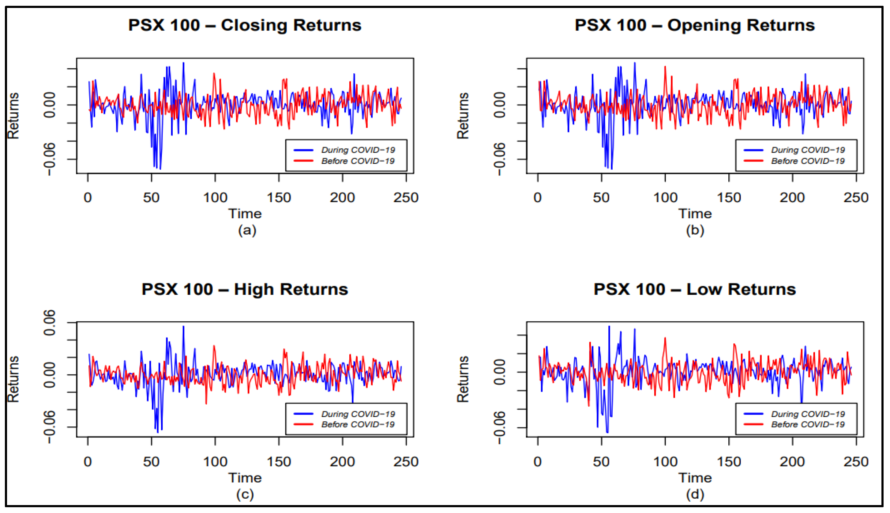
The Ljung–Box (LB) test shows no serial correlation exists in either time series. We have tested each data series for the ARCH effect. The langrage multiplier (LM) statistics shows the presence of the ARCH effect in all the data series shown in Table 2. ARCH-LM test uses F-statistic and chi-square statistic to determine the presence of the ARCH effect. It assumes that no ARCH effect exists in the null hypothesis. The p values of test statistics less than 1% recommends the rejection of the null hypothesis. In our case, most of the p values of both test statistics are less than 1%. Additionally, the excess kurtosis, skewness, and tests of non-normality have already validated the use of ARCH models. Figure 1 shows returns dynamics of PSX-100.

3.3. Volatility Estimation Using GARCH Models

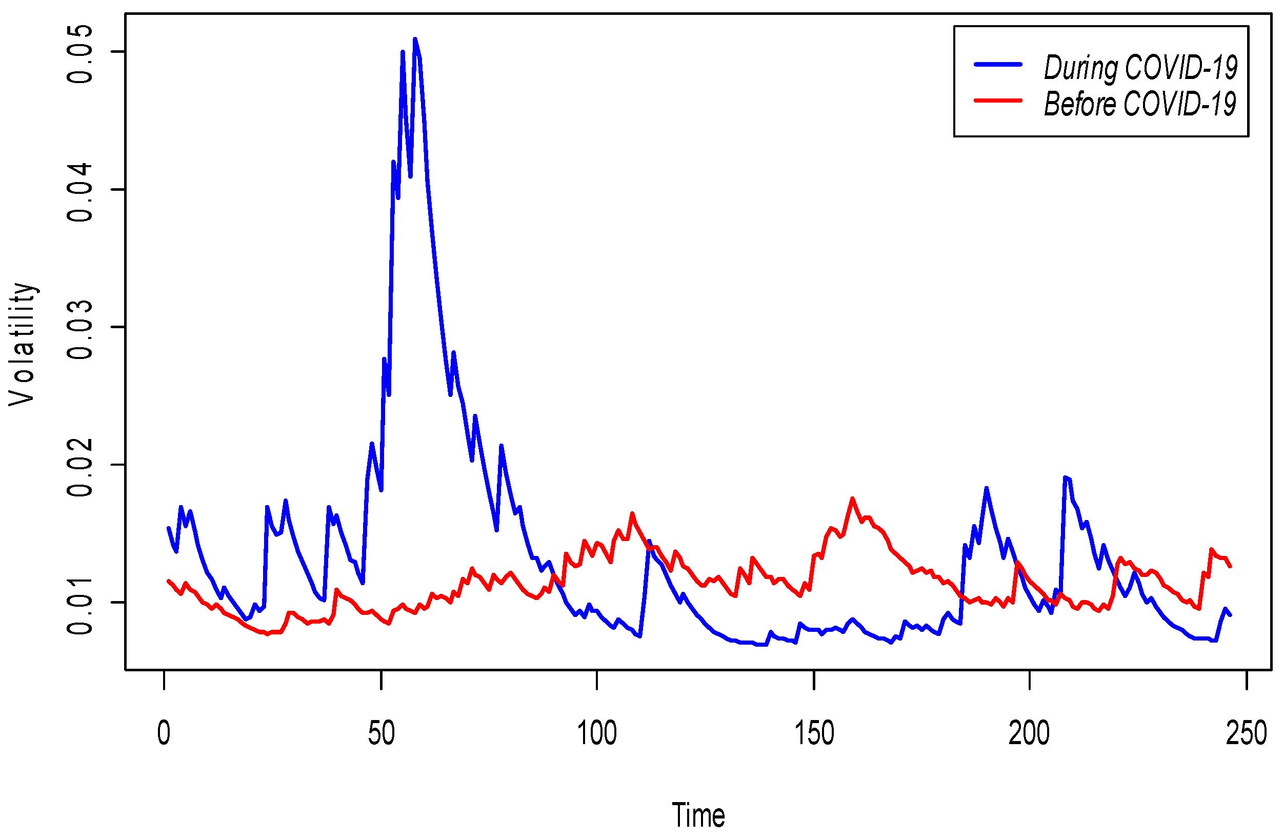
We estimated GJR-GARCH (1,1), EGARCH (1,1), and TGARCH (1,1) models using the Normal, STD, SSTD, GED, and SGED. We model and estimate the volatility of closed returns for two selected periods. The estimated volatilities are shown in Figure 2. We compared our estimation of volatilities using Levene’s test. The test results in the rejection of the null hypothesis with a p-value of 5.707 × 10⁻¹². We conclude that the volatility dynamics of PSX-100 closed returns during the COVID-19 pandemic is significantly higher. Figure 2 shows a clear picture of the variation between the volatilities of the two periods.

The estimated best-fitted in-sample volatility model’s parameters for the two underlying periods are shown in

Table 3. Best-fitted GARCH models parameters of PSX-100 closed-returns for two periods.

GJR-GARCH-SGED COVID-19 Period
mu	ar1	ma1	$\omega$	${\alpha }_1$	${\beta }_1$	${\gamma }_1$	skew	shape
0.0002 (0.0010)	0.8163 (0.1413)	−0.7490 (0.1661)	0.0000 (0.0000)	0.0000 (0.0126)	0.8222 (0.0312)	0.2437 (0.0820)	0.8801 (0.1162)	1.6361 (0.3015)
EGARCH-STD before-COVID-19 Period
	mu	ar1	ma1	$\omega$	${\alpha }_1$	${\beta }_1$	${\gamma }_1$	shape
	−0.0013 (0.0000)	−0.1308 (0.0000)	0.3022 (0.0000)	−0.1310 (0.0000)	−0.1792 (0.0000)	0.9854 (0.0001)	−0.1452 (0.0000)	18.7972 (0.0030)

. We have considered log-likelihood and information criteria, AIC, BIC, SIC, and HQIC, to determine the best-fit model selection. GJR-GARCH (1,1) model with SGED has found to be the best-fitted model for the pandemic period of COVID-19. The positive value of parameter ${\gamma }_1$ indicates the existence of the leverage effect. Therefore, we can conclude that investors in PSX-100 overreacted to the negative news during the pandemic, and volatility has responded more toward the negative shocks. Hence, the presence of the asymmetric effect is apparent.

Similarly, for PSX-100 closed returns series before the COVID-19 period, EGARCH (1,1) model with STD distribution is the best fit GARCH model.

We have found a high level of significant volatility persistence (0.9854), indicating that once a shock introduced to PSX-100 before the COVID-19 period, it takes time to die out. Therefore, it has a long memory. The coefficient of the leverage effect is negative (−0.1452) and significant. It shows the market behaves asymmetrically, and a negative relationship exists between the past returns and the current conditional variance. Consequently, the effect of a bad-news on the future volatility of the PSX-100 returns is higher than the good-news. Both GJR-GARCH (1,1) and EGARCH (1,1) models show the notable existence of the leverage effect.

Table A1. GARCH model selection of PSX-100 closed returns during COVID-19 pandemic.

Model	LOGLIK.	BIC	SIC	HQIC	AIC
Student T
GJRGARCH	745.2045	−5.9935	−5.8795	−5.9956	−5.9476
EGARCH	741.4358	−5.9629	−5.8489	−5.9649	−5.917
TGARCH	740.9011	−5.9585	−5.8446	−5.9606	−5.9126
Asymmetric Student T
GJRGARCH	746.4149	−5.9952	−5.867	−5.9978	−5.9436
EGARCH	742.1684	−5.9607	−5.8325	−5.9633	−5.9091
TGARCH	741.6314	−5.9564	−5.8281	−5.9589	−5.9047
Generalized Error
GJRGARCH	745.4326	−5.9954	−5.8814	−5.9974	−5.9495
EGARCH	742.1894	−5.969	−5.855	−5.971	−5.9231
TGARCH	741.8362	−5.9661	−5.8522	−5.9682	−5.9202
Skewed GED
GJRGARCH	746.4959	−5.9959	−5.8677	−5.9985	−5.9443
EGARCH	742.675	−5.9648	−5.8366	−5.9674	−5.9132
TGARCH	742.3509	−5.9622	−5.834	−5.9648	−5.9106

and

Table A2. GARCH model selection of PSX-100 closed returns before COVID-19 pandemic.

Model	LOGLIK.	BIC	SIC	HQIC	AIC
Student T
GJRGARCH	611.1641	−6.1547	−6.0209	−6.1579	−6.1006
EGARCH	611.0953	−6.1438	−5.9933	−6.1478	−6.0829
TGARCH	611.8439	−6.1617	−6.0279	−6.1648	−6.1075
Asymmetric Student T
GJRGARCH	612.1173	−6.1543	−6.0037	−6.1582	−6.6851
EGARCH	615.0001	−6.1939	−6.0601	−6.197	−6.1075
TGARCH	614.4997	−6.1786	−6.028	−6.1825	−6.0933
Generalized Error
GJRGARCH	616.2783	−6.2069	−6.0731	−6.2101	−6.1075
EGARCH	616.9883	−6.204	−6.0534	−6.2079	−6.0933
TGARCH	612.136	−6.1647	−6.0309	−6.1678	−6.1397
Skewed GED
GJRGARCH	612.2701	−6.1558	−6.0053	−6.1598	−6.0933
EGARCH	612.6194	−6.1696	−6.0358	−6.1727	−6.1397
TGARCH	613.2739	−6.1661	−6.0155	−6.1700	−6.1176

in Appendix A show values of log-likelihoods, AIC, BIC, SIC, and HQIC for best-fitted GARCH models.

3.4. Volatility Assessment Using Shannon and Tsallis Entropy

In this section, we use closing prices and two estimated volatility series of PSX-100 closing returns. Each series contains 250 estimated volatilities. We have investigated in the previous Section that GJR-GARCH (1,1) fits best for the pre-pandemic period, and during the pandemic, EGARCH (1,1) resulted as the best-fitted volatility model. We compute the regularity and diversity of both estimated volatility series by using four different entropy measures. The efficient market hypothesis indicates high values of entropy shows randomness in the dynamics of the stock prices. We have used Shannon’s entropy, Tsallis entropy, ApEn, and SampEn to enhance our understanding of the estimated volatility series and closing prices of PSX-100.

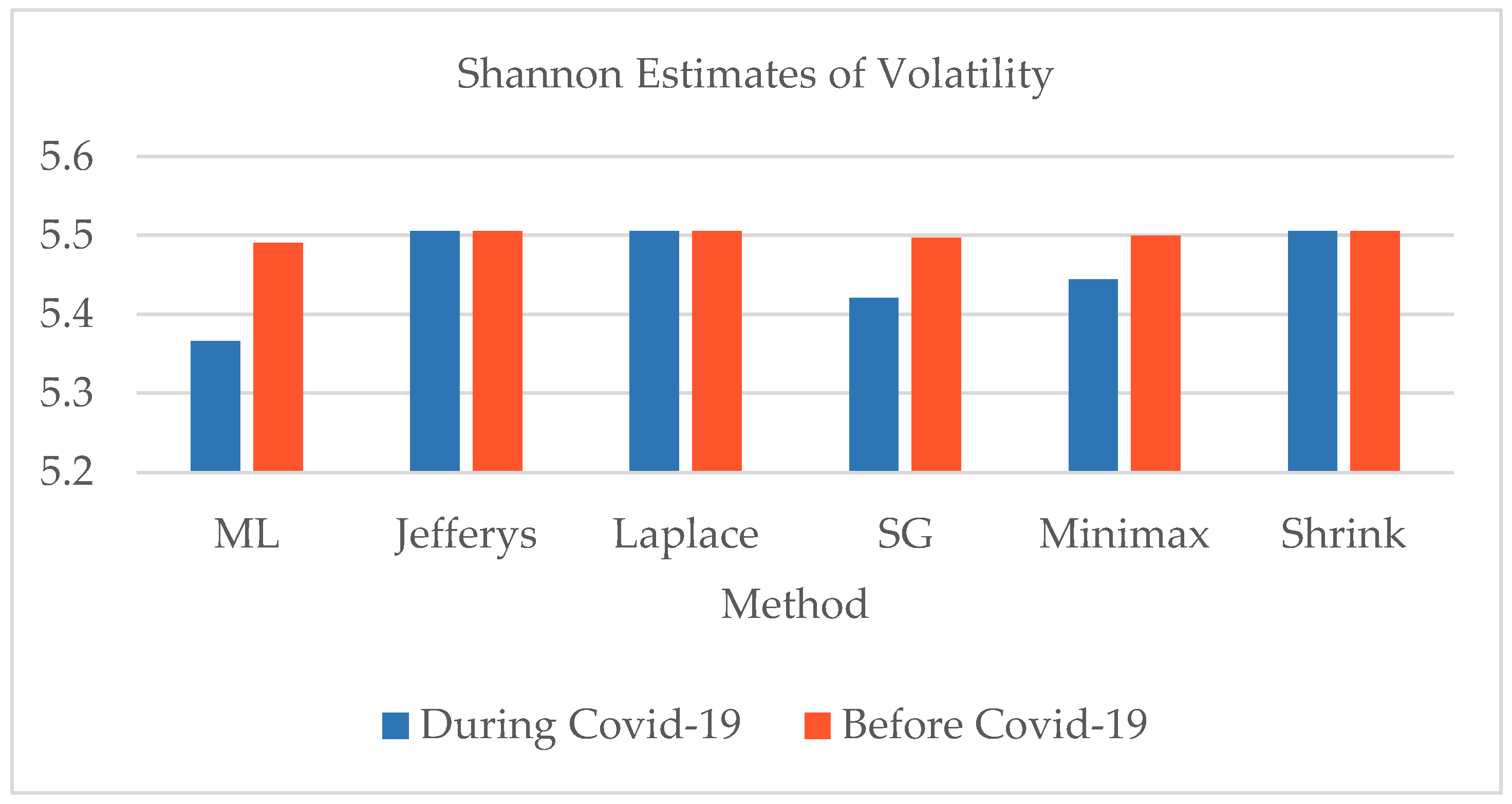
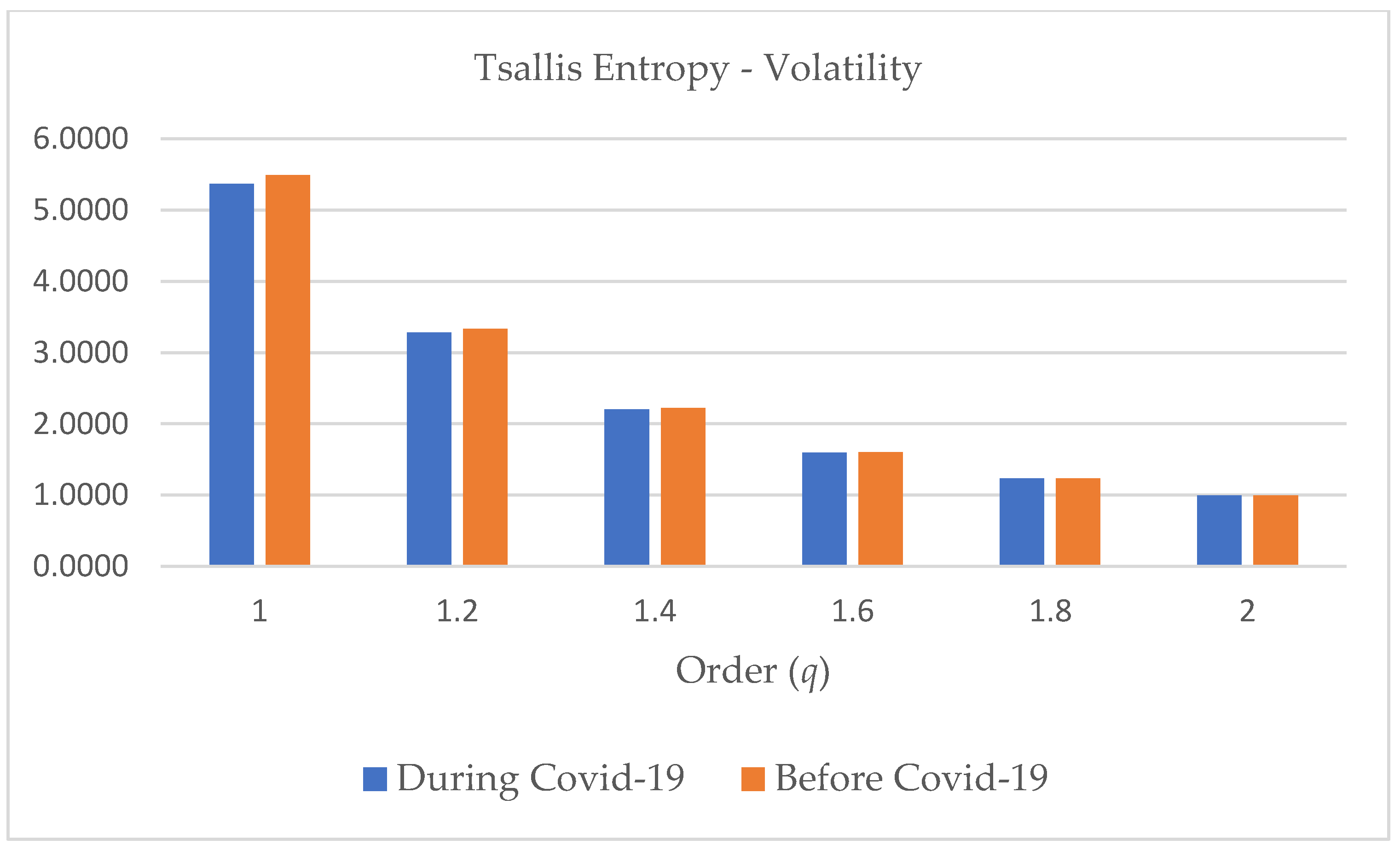
We use the Shannon entropy, using several estimators, to evaluate the consistency of our results. We have noticed a very slight change in Shannon’s entropy for both pre-pandemic and pandemic periods for the estimated volatility series. Surprisingly, the pandemic period is 2% less volatile than the pre-pandemic period. The Shannon entropy estimates of closing prices show similar behavior under all the estimation methods. The large values of closing prices and their low variation cause a similar pattern of computed entropies. For q approaching 1, the Tsallis entropy converges to the Shannon, and entropies become very low for frequently encountered events ($q>1)$. We have found both entropies are positive for the underlying two volatility series. Therefore, volatility shows non-linear behavior. We investigated that the overall relative difference of entropies between the two periods is not noticeable.

Table 4. Estimates of the Shannon entropy for PSX-100 estimated volatilities and closing prices.

Estimation	Volatility		Prices
Method	COVID-19	Before COVID-19	COVID-19	Before COVID-19
ML	5.3661	5.4902	5.5037	5.5050
Jeffreys	5.5052	5.5053	5.5037	5.5050
Laplace	5.5053	5.5053	5.5037	5.5050
SG	5.4207	5.4971	5.5037	5.5050
minimax	5.4439	5.4994	5.5037	5.5050
Shrink	5.5053	5.5053	5.5037	5.5050

shows Shannon’s entropy estimates of the underlying volatility series and closing prices of PSX-100. The results of the Tsallis entropy estimates for the same data series are given in

Table 5. Estimates of Tsallis entropy for PSX-100 estimated volatilities and closing prices.

Parameter	Volatility		Prices
q	COVID-19	Before COVID-19	COVID-19	Before COVID-19
1	5.3661	5.4902	5.5037	5.5050
1.2	3.2792	3.3314	3.3365	3.3370
1.4	2.1998	2.2212	2.2232	2.2234
1.6	1.5958	1.6045	1.6052	1.6053
1.8	1.2309	1.2344	1.2346	1.2347
2	0.9944	0.9958	0.9959	0.9959

. See Figure 3 and Figure 4 to visualize the Shannon entropy estimates and Tsallis entropy estimates. The pre-pandemic period spans from 1 January 2019 to 31 December 2019. The pandemic period spans from 1 January 2020 to 24 December 2020. In the case of Shannon’s entropy for volatility series, the Jefferys, Laplace, and Shrink estimators are found consistent.

3.5. Regularity and Randomness Using Approximate Entropy and Sample Entropy

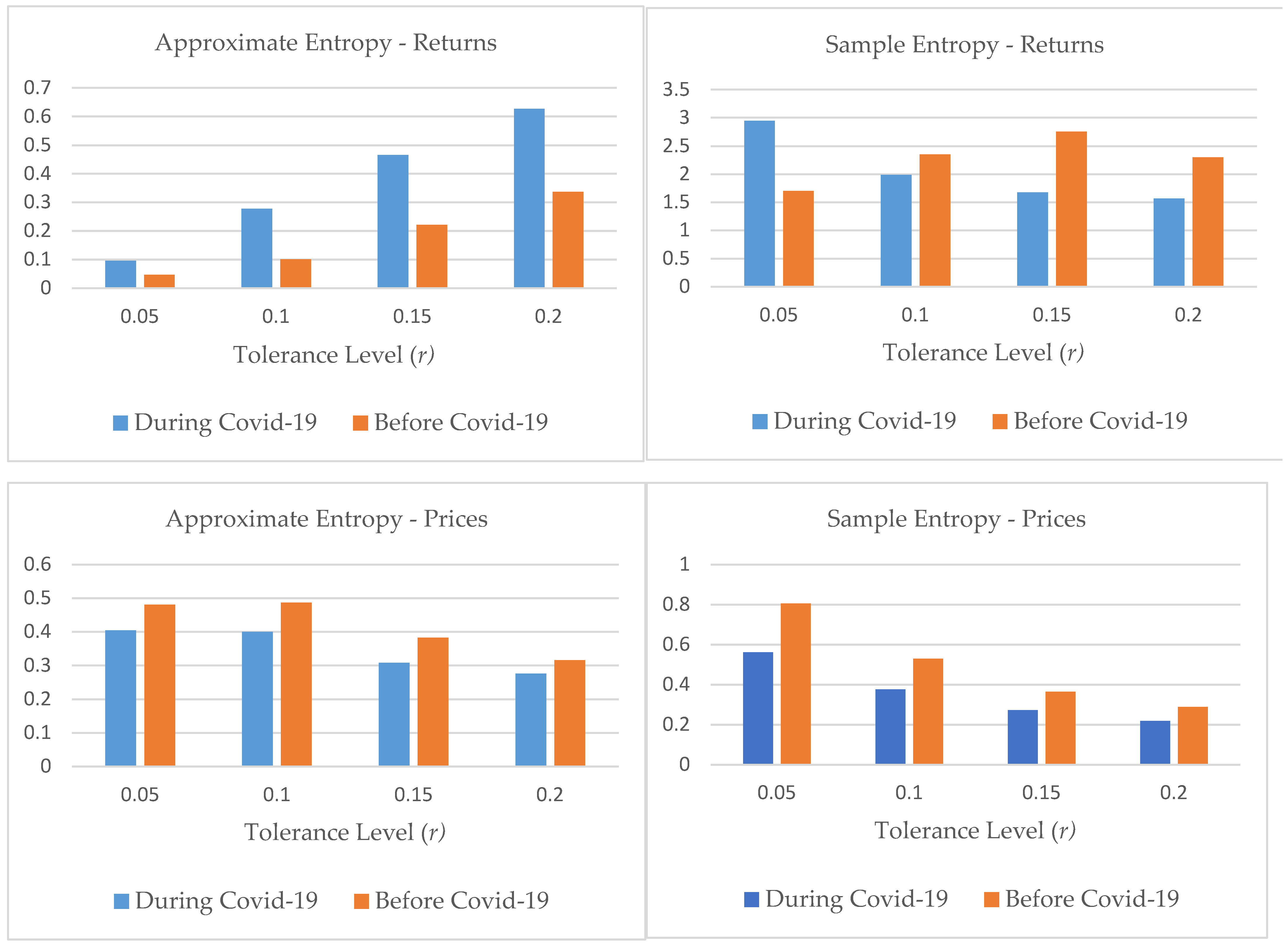
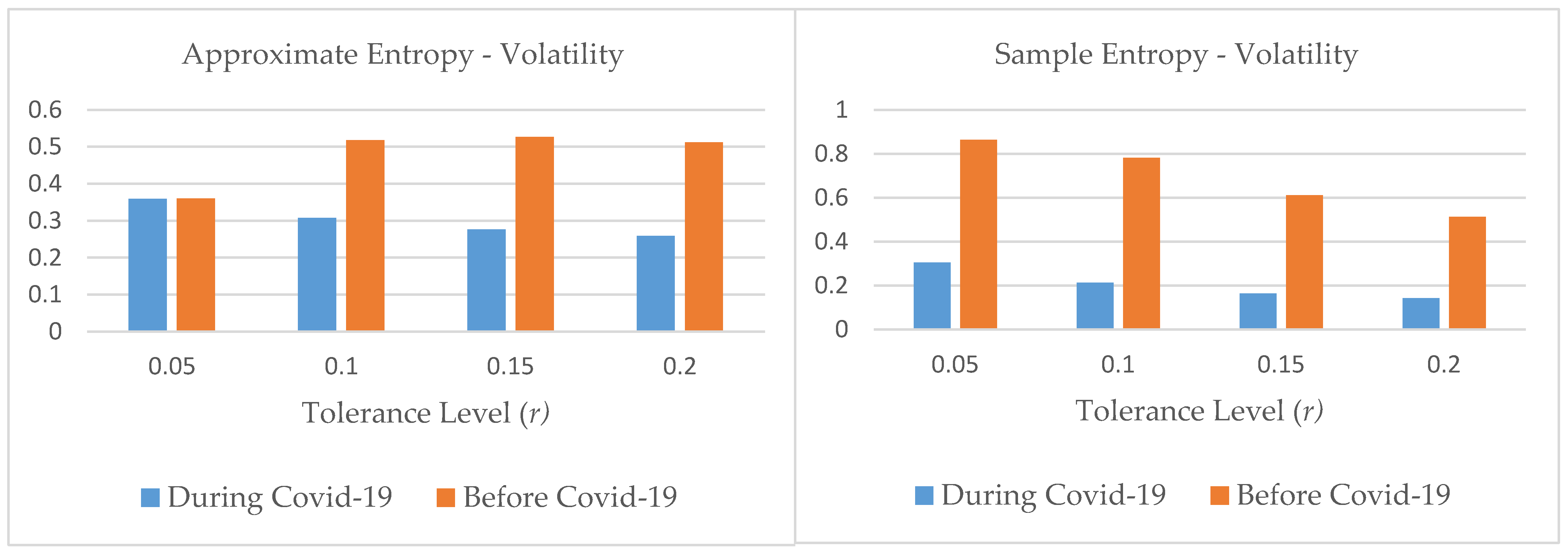
We implement ApEn for the quantification of regularity and characterization of the degree of randomness. However, volatility (standard deviation) describes the extent of departure from the mean. The ApEn and SampEn are similar algorithms, but ApEn is extremely sensitive to its input parameters. The standard deviation of the pre-pandemic estimated volatility series is 0.0019, and during the pandemic is 0.00802, the tolerance-level r is selected in the range $\left[0.1\widehat{\sigma },0.25\widehat{\sigma }\right]$, where $\widehat{\sigma }$ denotes the sample standard deviation. We set $l=1,2,3$ and $r=0.05\widehat{\sigma }$ , $0.1\widehat{\sigma }$, $0.15\widehat{\sigma }$, and $0.20\widehat{\sigma }$. A similar procedure has followed for the computation of closing prices and closing returns series of PSX-100. We have analyzed small values of ApEn and SampEn for the estimated volatility series of the pandemic period. These results reflect relatively high persistence, strong dependence, and predictability of volatility. On the other hand, ApEn shows more randomness for closing returns of the PSX-100 during the pandemic period. We have noticed that ApEn is significantly sensitive to the choice of tolerance level r and dimension l. The sample entropy results distinctly suggest that the pre-pandemic period was more random and volatile. See

Table 6. Estimates of the approximate entropy for estimated volatility, closing prices, and closing returns of PSX-100.

$\mathit{r}$	$\mathit{l}$	Returns		Volatility		Prices
		COVID-19	Before COVID-19	COVID-19	Before COVID-19	COVID-19	Before COVID-19
0.05	1	2.0077	1.9918	0.5665	1.051	0.8225	0.876
	2	0.6347	0.5192	0.475	0.7457	0.5948	0.6834
	3	0.0958	0.047	0.3587	0.3605	0.4043	0.4813
0.1	1	1.9011	2.0217	0.4579	0.9009	0.5764	0.5923
	2	0.9052	0.7616	0.3918	0.7500	0.482	0.565
	3	0.2774	0.1014	0.3073	0.5177	0.3998	0.4872
0.15	1	1.7757	1.9621	0.4091	0.7828	0.4231	0.4143
	2	0.995	0.9847	0.3325	0.6667	0.3639	0.4258
	3	0.4658	0.222	0.2761	0.5267	0.3085	0.3828
0.2	1	1.6367	1.8465	0.3535	0.6795	0.3358	0.3074
	2	1.0500	1.1772	0.3105	0.6127	0.3141	0.3251
	3	0.6265	0.3374	0.2585	0.5123	0.2757	0.3164

and

Table 7. Estimates of the approximate entropy for estimated volatility, closing prices, and closing returns of PSX-100.

r	l	Returns		Volatility		Prices
		COVID-19	Before COVID-19	COVID-19	Before COVID-19	COVID-19	Before COVID-19
0.05	1	2.4511	2.6077	0.3638	1.0016	0.7022	0.8336
	2	2.3931	2.4849	0.3316	1.0452	0.613	0.8029
	3	2.9444	1.7047	0.3039	0.8627	0.5625	0.8052
0.1	1	2.0316	2.4002	0.2712	0.7824	0.4747	0.5476
	2	1.875	2.4022	0.2397	0.8176	0.4061	0.5454
	3	1.9879	2.3514	0.2128	0.7807	0.3757	0.5301
0.15	1	1.7655	2.165	0.2215	0.6359	0.3431	0.385
	2	1.5924	2.1313	0.19	0.6476	0.2913	0.3878
	3	1.678	2.7515	0.1632	0.6107	0.2723	0.3644
0.2	1	1.5554	1.9543	0.1939	0.5431	0.271	0.2969
	2	1.434	2.0363	0.1655	0.5518	0.2335	0.2982
	3	1.5666	2.3026	0.143	0.5125	0.2184	0.2895

, and Figure 5.

4. Discussion and Conclusions

This study was concerned with investigating the volatility dynamics of the Pakistan Stock Exchange. We employed the most widely used traditional technique of GARCH modeling to estimate the volatilities of data sets divided into pre-pandemic and pandemic periods of COVID-19. For this purpose, we chosen univariate conditional volatility models, namely GJR-GARCH, TGARCH and EGARCH. These models have been significantly used to estimate and forecast the volatility. Additionally, these models capture asymmetry and leverage effect, which is the negative correlation between returns shocks and consequent volatility shocks. We have examined a different behavior of the estimated volatility series of the pre-pandemic period and the pandemic period. Based on our results, we accept the hypothesis H1. Therefore, the volatility market of PSX-100 daily closed returns has increased during the pandemic period with the notable existence of the leverage effect. The GJR-GARCH (1,1) model with SGED best fits the pandemic period, and investors of the market have overreacted to the negative news. Resultantly, volatility responded more strongly towards the negative shocks. The EGARCH (1,1) model with Student t-distribution best fits the pre-pandemic period. Therefore, we have found volatility persistence, long-memory, and the existence of the leverage effect. We summarize results based on GARCH modeling as follows.

• Both best-fitted models suggested the remarkable existence of the leverage effect in the Pakistan Stock Exchange;
• A high variation in the estimated volatility of the pandemic period has observed, and extreme downturns in prices are expected;
• The behavior of the variance is asymmetric for PSX-100 closing returns of both examined periods;
• The GARCH volatility modeling shows a usual behavior of the Pakistani market response towards bad news.

The choice of the conditional distribution in GARCH type modeling is a critical step. It leads to the limitation of the study, and as a result, the selection of the best-fitted model is significantly dependent on the underlying residual distribution. Our findings and literature review show that the returns distributions show fat-tailed non-Gaussian behavior. Therefore, the central limit theorem does not apply to financial time series. Resultantly, one may check whether the returns are sequentially independent or not. On other hand, the GARCH family model’s estimation involves several crucial steps such as appropriateness of the selected model, parameters estimation, identification of the order of the model’s parameters p and q.

Alternatively, the information-theoretic approach does not cause any restriction on the theoretical probability distribution, and the underlying stochastic process can be characterized through quantification of randomness and uncertainty. Consequently, this approach provides a more direct way of similar computations to GARCH modeling.

Our findings based on the Shannon entropy, Tsallis entropy, approximate entropy, and sample entropy reveal different behavior of the estimated volatilities, closing prices and closing returns series of PSX-100. We summarize the results based on information measures as follows.

• We have pointed out that no remarkable difference between the randomness of volatility series before and during the COVID-19 pandemic, based on Shannon and Tsallis entropy estimates;
• All values of entropies are positive on both periods, and volatility shows non-linear dynamics;
• The overall relative difference of estimated entropies is not significant;
• The overall relative difference of estimated entropies is not significant under both the Shannon and Tsallis entropies;
• In the case of closing prices of the PSX-100, the Shannon entropy shows almost similar behavior under all estimation methods;
• In the case of ApEn and SampEn, the market shows mixed behavior, and the results are more sensitive. The sample entropy results reported more randomness in the pre-pandemic period for the Pakistani Stock Market. We detected both entropies are very sensitive to the selection of parameters.

Our research carried out in this framework demonstrated that information-based approaches are simpler and provide results aligned with the best performance of the Pakistan market in Asia during the pandemic. Our findings show that randomness of the PSX-100 estimated volatilities, closing prices and closing returns was not high during the pandemic COVID-19. We selected PSX-100 for empirical analysis because of its best performance in the region and other world markets. There was a clear research gap on the underlying market. We aimed to fill the existing research gap on the most emerging and best performer market of Asia. Our goal of the study was not a detailed analysis of the volatility. Many papers exist in the literature on estimating and predicting the volatility of PSX-100. See, for example, Ahmed et al. (2016); Joyo and Lin (2019); Umar et al. (2021). On the other hand, Liu et al. (2021) studied the impact of COVID-19 to estimate the conditional skewness of the return distribution from a GARCH-S model as the proxy for the equity market crash risk of the Shanghai Stock Exchange. Waheed et al. (2020) also confirmed in their study that PSX-100 has positive increments in returns during the pandemic. Lahmiri and Bekiros (2020a) used a simple GARCH model, Wavelet packet Shannon entropy and hierarchical clustering for a short data set of four months of several equity groups. We investigated the effectiveness of our new approaches based on entropy measures and comparison to frequently used GARCH modeling. Our entropy-based results also conclude that the Pakistani market performed better during the pandemic. Additionally, entropy measures such as approximate entropy and sample entropy performed well for a data set at least equal to 200. See, for example, Yentes et al. (2012); one of the reasons to consider the one-year data set as sufficient for our empirical analysis and fulfilled the methodologic requirement of entropy methods. In addition to this, based on our information-theoretic results, the Pakistani market performed better during the pandemic. Lastly, in our future papers, we will investigate and extend our study for (a) longer periods, (b) more assets or representative indices, and (c) inter-country analysis.

References

- Abdalla, Suliman Zakaria Suliman, and Zakaria Suliman. 2012. Modelling stock returns volatility: Empirical evidence from Saudi Stock Exchange. International Research Journal of Economics 85: 166–79. [Google Scholar]
- Ahmed, Nawaz, Rizwan Raheem Ahmed, Jolita Vveinhardt, and Dalia Streimikiene. 2016. Empirical analysis of stock returns and volatility: Evidence from Asian stock market. Technological and Economic Development of Economy 22: 808–29. [Google Scholar]
- Ahn, Kwangwon, Daeyong Lee, Sungbin Sohn, and Biao Yang. 2019. Stock Market Uncertainty and Economic Fundamental: An Entropic Based Approach. Quantitative Finance 19: 1151–63. [Google Scholar] [CrossRef]
- Alamgir, Farzana, and Sakib Bin Amin. 2021. The nexus between oil price and stock market: Evidence from South Asia. Energy Reports 7: 693–703. [Google Scholar] [CrossRef]
- Ali, Rizwan, Inayat Ullah Mangla, Ramiz Ur Rehman, Wuzhao Xue, Muhammad Akram Naseem, and Muhammad Ishfaq Ahmad. 2020. Exchange rate, gold price, and stock market nexus: A quantile regression approach. Risks 8: 86. [Google Scholar] [CrossRef]
- Andersen, Torben G., Tim Bollerslev, Francis X. Diebold, and Paul Labys. 2001. The distribution of realized exchange rate volatility. Journal of American Statistical Association 96: 42–57. [Google Scholar] [CrossRef]
- Aruga, Kentaka. 2021. Changes in human mobility under the COVID-19 pandemic and the Tokyo fuel market. Journal of Risk and Financial Management 14: 163. [Google Scholar] [CrossRef]
- Bali, Turan G, and Panayiotis Theodossiou. 2006. A Conditional-SGT-VaR Approach with alternative GARCH models. Annals of Operations Research 151: 241–67. [Google Scholar] [CrossRef]
- Bartiromo, Rosario. 2010. Shared information in the stock market. Quantitative Finance 11: 229–35. [Google Scholar] [CrossRef]
- Bentes, Sonia R., and Rui Menezes. 2012. Entropy A New Measure of Stock Market Volatility. Journal of Physics: Conference Series 394: 012033. [Google Scholar] [CrossRef]
- Bhowmik, Roni, and Shouyang Wang. 2020. Stock market volatility and return analysis: A systematic literature review. Entropy 22: 522. [Google Scholar] [CrossRef]
- Bollerslev, Tim. 1986. Generalized autoregressive conditional heteroskedasticity. Journal of Econometrics 31: 307–327. [Google Scholar] [CrossRef] [Green Version]
- Bollerslev, Tim. 1987. A conditionally heteroskedastic time series model for speculative prices and rates of return. Review of Economics and Statistics 69: 542–47. [Google Scholar] [CrossRef] [Green Version]
- Cao, Charles Q., and Ruey S. Tsay. 1992. Nonlinear time-series analysis of stock volatilities. Journal of Applied Econometrics 7: S165–S185. [Google Scholar] [CrossRef]
- Chkili, Walid, Chaker Aloui, and Duc K. Nguyen. 2012. Asymmetric effects and long memory in dynamic volatility relationships between stock returns and exchange rates. Journal of International Financial Markets, Institutions and Money 22: 738–57. [Google Scholar] [CrossRef]
- Darbellay, Georges A., and Diethelm Wuertz. 2000. The entropy as a tool for analyzing statistical dependence in financial time series. Physica A 287: 429–39. [Google Scholar] [CrossRef]
- Dhanaiah, Gangineni, and Siviram R. Prasad. 2017. Volatility and co-movement models: A literature review and synthesis. International Journal of Engineering Management Research 7: 1–25. [Google Scholar]
- Ding, Zhuanxin, Clive WJ Granger, and Robert F. Engle. 1993. A long memory property of stock market returns and a new model. Journal of Empirical Finance 1: 83–106. [Google Scholar] [CrossRef]
- Engle, Robert.F. 1982. Autoregressive conditional heteroscedasticity with estimates of the variance of United Kingdom inflation. Econometrica 50: 987–1007. [Google Scholar] [CrossRef]
- Fan, Ying, Yu-Jun Zhang, Hsein-Tang Tsai, and Yi-Ming Wei. 2008. Estimating ‘value at risk’ of crude oil price and its spillover effect using the ged-garch approach. Energy Economics 30: 3156–71. [Google Scholar] [CrossRef]
- Figlewski, Stephen. 1997. Forecasting volatility. Financial Markets, Institutions, and Instruments 6: 1–88. [Google Scholar] [CrossRef]
- Figlewski, Stephen, and Clifton T. Green. 1999. Market risk and model risk for a financial institution writing options. Journal of Finance 54: 1465–999. [Google Scholar] [CrossRef] [Green Version]
- Francq, Christian, and Jean-Michel Zakoian. 2010. GARCH Models:Structure, Statistical Inferences and Financial Applications. West Sussex: Wiley. [Google Scholar]
- Gell-Mann, Murray, and Constantino Tsallis. 2004. Nonextensive Entropy: Interdisciplinary Applications. Oxford: Oxford University Press. [Google Scholar]
- Gençay, Ramaza, and Nikola Gradojevic. 2008. Overnight interest rates and aggregate market expectations. Economic Letters 100: 27–30. [Google Scholar]
- Gençay, Ramazan, and Nikola Gradojevic. 2010. Crash of 087—Was it expected? Aggregate market fears and long-range dependence. Journal of Empirical Finance 17: 270–82. [Google Scholar] [CrossRef]
- Gençay, Ramaza, and Nikola Gradojevic. 2017. The Tale of Two Financial Crises: An Entropic Perspective. Entropy 19: 244. [Google Scholar] [CrossRef]
- Glosten, Lawrence R., Ravi Jagannathan, and David E. Runkle. 1993. On the relation between the expected value and the volatility of the nominal excess return on stocks. Journal of Finance 48: 1779–801. [Google Scholar] [CrossRef]
- Gosset, William Sealy. 1908. The probable error of a mean. Biometrika 6: 1–25. [Google Scholar]
- Gulko, Less. 1999. The entropy theory of stock option pricing. International Journal of Theoretical and Applied Finance 2: 331–55. [Google Scholar] [CrossRef]
- Harrison , Barry, and Winston R. Moor. 2012. Forecasting stock market volatility in central and eastern European countries. Journal of Forecasting 31: 490–503. [Google Scholar] [CrossRef]
- Hansen, Bruce E. 1994. Autoregressive conditional density estimation. International Economic Review 35: 705–30. [Google Scholar] [CrossRef]
- Hussain, Sartaj, Bhanu K. V. Murthy, and Amit Kumar Singh. 2019. Stock market volatility: A review of the empirical literature. IUJ Journal of Management 7: 96–105. [Google Scholar]
- Joyo, Ahmed Shafique, and Lin Lefin Lin. 2019. Stock Market Integration of Pakistan with Its Trading Partners: A Multivariate DCC-GARCH Model Approach. Sustainability 11: 303. [Google Scholar] [CrossRef] [Green Version]
- Kolmogorov, Andrei Nikolaevich. 1958. A New Metric Invariant of Transient Dynamical Systems and Automorphisms in Lebesgue Spaces. Doklady Akademii Nauk, Russian Academy of Sciences: Moscow, Russai 119: 861–64. [Google Scholar]
- Lahmiri, Salim, and Stelios Bekiros. 2020a. Randomness, Informational Entropy, and Volatility Interdependencies among the Major World Markets: The Role of the COVID-19 Pandemic. Entropy 22: 833. [Google Scholar] [CrossRef] [PubMed]
- Lahmiri, Salim, and Stelios Bekiros. 2020b. Nonlinear analysis of Casablanca Stock Exchange, Dow Jones and S&P500 industrial sectors with a comparison. Physica A 539: 122923. [Google Scholar]
- Lambert, Philippe, and Sebastien Laurent. 2001. Modleing Financial Time Series Using Garch-Type Models and a Skewed-Student t-Density. Ottignies-Louvain-la-Neuve: Universit’e Catholique de Louvain, Institut de Statistique. [Google Scholar]
- Lee, Gary G. J., and Robert F. Engle. 1999. A permanent and transitory component model of stock return volatility. In Cointegration Causality and Forecasting A Festschrift in Honor of Clive WJ Granger. New York: Oxford University Press, pp. 475–97. [Google Scholar]
- Liu, Zhifeng, Toan Luu Duc Huynh, and Peng-Fei Dai. 2021. The impact of COVID-19 on the stock market crash risk in China. Research in international Business and Finance 57: 101419. [Google Scholar] [CrossRef]
- Mabrouk, Samir, and Samir Saadi. 2012. Parametric value-at-risk analysis: Evidence from stock indices. The Quarterly Review of Economics and Finance 52: 305–321. [Google Scholar] [CrossRef]
- Mandelbort, Benoit. 1963. The Variation of Certain Speculative Prices. The Journal of Business 36: 394–419. [Google Scholar] [CrossRef]
- McMillan, David N., Alan Speight, and Owain Apgwilym. 2000. Forecasting UK stock market volatility. Applied Financial Economics 10: 435–48. [Google Scholar] [CrossRef]
- Mensi, Walid. 2013. Ranking efficiency for twenty-six emerging stock markets and financial crisis: Evidence from the Shannon entropy approach. International Journal of Management Science and Engineering 7: 53–63. [Google Scholar] [CrossRef]
- Nelson, Daniel B. 1991. Conditional heteroskedasticity in asset returns: A new approach. Economics 59: 347–70. [Google Scholar] [CrossRef]
- Ng, Hock Guan, and Michael McAleer. 2004. Recursive modelling of symmetric and asymmetric volatility in the presence of extreme observations. International Journal of Forecasting 20: 115–29. [Google Scholar] [CrossRef]
- Okicic, Jasmina. 2015. An empirical analysis of stock returns and volatility: The case of stock markets from Central and Eastern Europe and South East. European Journal of Economics Business 9: 7–15. [Google Scholar] [CrossRef] [Green Version]
- Ong, Marcus A. 2015. An information theoretic analysis of stock returns, volatility and trading volumes. Applied Economics 47: 3891–906. [Google Scholar] [CrossRef]
- Patev, Plamen, and Nigokhos Kanaryan. 2008. Stock Market Volatility Changes in Central Europe Caused by Asian and Russian Crisis. International Journal of Economic Research 5: 13–35. [Google Scholar]
- Pele, Daniel Traian, Emese Lazar, and Alfonso Dufour. 2017. Information entropy and measure of market risk. Entropy 19: 226. [Google Scholar] [CrossRef] [Green Version]
- Pincus, Steven M. 1991. Approximate entropy as a measure of system complexity. Proceedings of the National Academy of Sciences of the United States of America 88: 2297–301. [Google Scholar] [CrossRef] [Green Version]
- Pincus, Steve M. 2008. Approximate Entropy as an Irregularity Measure for Financial Data. Econometric Reviews 27: 329–62. [Google Scholar] [CrossRef]
- Poon, Ser-Huang, and Clive Granger. 2005. Practical issues in forecasting volatility. Financial Analysts Journal 61: 45–56. [Google Scholar] [CrossRef] [Green Version]
- Preda, Vasile, and Costel Balcau. 2010. Entropy Optimization with Applications. Bucharest: The Publishing House of the Romanian Academy. [Google Scholar]
- Preda, Vasile, and Muhammad Sheraz. 2015. Risk-neutral densities in entropy theory of stock options using Lambert function and a new approach. Proceedings of The Romanian Academy Series A 16: 20–27. [Google Scholar]
- Preda, Vasile, Silvia Dedu, and Muhammad Sheraz. 2014. New measure selection for Hunt-Devolder semi-Markov regime switching interest rate models. Physica A: Statistical Mechanics and Its Applications 407: 350–59. [Google Scholar] [CrossRef]
- Rényi, Alfred. 1961. On measures of entropy and information. In Proceedings of the 4th Berkely Sympodium on Mathematics of Statistics and Probability. Berkeley: University of California Press, vol. 1, pp. 547–61. [Google Scholar]
- Ribeiro, Maria, Teresa Henriques, Luísa Castro, André Souto, Luís Antunes, Cristina Costa-Santos, and Andreia Teixeira. 2021. The entropy Universe. Entropy 23: 222. [Google Scholar] [CrossRef] [PubMed]
- Richman, Joshua S., and J. Randall Moorman. 2000. Physiological time-series analysis using approximate entropy and sample entropy. American Journal of Physiology Heart and Circulatory Physiology 278: 2039–49. [Google Scholar] [CrossRef] [Green Version]
- Shannon, Claude E. 1948. A mathematical theory of communication. The Bell System Technical Journal 27: 379–423. [Google Scholar] [CrossRef] [Green Version]
- Sheraz, Muhammad, Silvia Dedu, and Vasile Preda. 2015. Entropy measures for assessing volatile markets. Procedia Economics and Finance 22: 655–62. [Google Scholar] [CrossRef] [Green Version]
- Sheraz, Muhammad, Vasile Preda, and Silvia Dedu. 2019. Non-Extensive Minimal Entropy Martingale Measures, and semi-Markov Regime Switching Interest Rate Modeling. AIMS Mathematics 5: 300–10. [Google Scholar] [CrossRef]
- Szczygielski, Jan Jakub, Princess Rutendo Bwanya, Ailie Charteris, and Janusz Brzeszczyński. 2021. The only certainty is uncertainty: An analysis of the impact of COVID-19 uncertainty on regional stock markets. Finance Research Letters, 101945. [Google Scholar] [CrossRef] [PubMed]
- Tapiero, Oren J. 2013. The relationship between risk and incomplete states uncertainty: A Tsallis entropy perspective. Algorithmic Finance 2: 141–50. [Google Scholar] [CrossRef] [Green Version]
- Taylor, Stephen J. 1986. Modelling Financial Time Series. Chichester: John Wiley & Sons Ltd. [Google Scholar]
- Taylor, Stephen J. 1987. Forecasting of the volatility of currency exchange rates. International Journal of Forecasting 3: 159–70. [Google Scholar] [CrossRef]
- Taylor, James W. 2004. Volatility forecasting with smooth transition exponential smoothing. International Journal of Forecasting 20: 273–86. [Google Scholar] [CrossRef]
- Toma, Aida. 2014. Model selection criteria using divergences. Entropy 16: 2686–98. [Google Scholar] [CrossRef] [Green Version]
- Topcu, Mert, and Omer Serkan Gulal. 2020. The impact of COVID-19 on emerging stock markets. Finance Research Letters 36: 101691. [Google Scholar] [CrossRef]
- Tsallis, Constantino. 1988. Possible generalization of Boltzmann-Gibbs statistics. Journal of Statistical Physics 52: 479–87. [Google Scholar] [CrossRef]
- Umar, Muhammad, Nawazish Mirza, Syed Kumail Abbas Rizvi, and Mehreen Furqan. 2021. Asymmetric Volatility Structure of Equity Returns: Evidence from an Emerging Market. The Quarterly Review of Economics and Finance. [Google Scholar] [CrossRef]
- Waheed, Rida, Suleman Sarwer, Sahar Sarwer, and Muhammad Kaleem Khan. 2020. The impact of COVID-19 on Karachi stock exchange: Quantileon-quantile approach using secondary and predicted data. Journal of Public Affairs 20: e2290. [Google Scholar] [CrossRef] [PubMed]
- Wiśniewska, Małgorzata, and Agnieszka Wyłomańska. 2017. A Garch process with ged distribution. In Cyclostationarity: Theory and Methods. Cham: Springer, vol. III, pp. 83–103. [Google Scholar]
- Xu, Libo. 2021. Stock Return and the COVID-19 pandemic: Evidence from Canada and the US. Finance Research Letters 38: 101872. [Google Scholar] [CrossRef]
- Yentes, Jennifer M., Nathaniel Hunt, Kendra K. Schmid, Jeffrey P. Kaipust, Denise McGrath, and Nicholas Stergiou. 2012. The appropriate use of approximate entropy and sample entropy with short data sets. Annals of Biomedical Engineering 41: 349–65. [Google Scholar] [CrossRef]
- Zakoian, Jean-Michel. 1994. Threshold heteroskedastic models. Journal of Economic Dynamics and Control 18: 931–55. [Google Scholar] [CrossRef]
- Zhou, Rongxi, Ru Cai, and Guanqun Tong. 2013. Applications of entropy in finance: A review. Entropy 15: 4909–31. [Google Scholar] [CrossRef]
- Zhu, Dongmin, and Jhon W. Galbraith. 2011. Modeling and forecasting expected shortfall with the generalized asymmetric student-t and asymmetric exponential power distributions. Journal of Empirical Finance 18: 765–78. [Google Scholar] [CrossRef]
- Zimon, Grzegorz, and Hossein Tarighi. 2021. Effects of the COVID-19 global crisis on the working capital management policy: Evidence from Poland. Journal of Risk Financial Management 14: 169. [Google Scholar] [CrossRef]
Figure 1.
Volatility clustering of PSX-100 returns.
Figure 2.
Comparison of estimated volatilities of PSX-100 returns. The pre-pandemic period spans from 1 January 2019 to 31 December 2019, and pandemic period spans from 1 January 2020 to 24 December 2020. This suggest that the COVID-19 affected significantly the PSX-100 volatility.
Figure 3.
The plot of Shannon entropy estimates for estimated volatility series of PSX-100.
Figure 4.
The plot of Tsallis entropy estimates for the two estimated volatility series of X-100.
Figure 5.
The plot of the approximate entropy and sample entropy estimates for estimated volatility series, closing prices and closing returns of PSX-100.