Monte Carlo Simulation of the Moments of a Copula-Dependent Risk Process with Weibull Interwaiting Time

Abstract

The widely used Poisson count process in insurance claims modeling is no longer valid if the claims occurrences exhibit dispersion. In this paper, we consider the aggregate discounted claims of an insurance risk portfolio under Weibull counting process to allow for dispersed datasets. A copula is used to define the dependence structure between the interwaiting time and its subsequent claims amount. We use a Monte Carlo simulation to compute the higher-order moments of the risk portfolio, the premiums and the value-at-risk based on the New Zealand catastrophe historical data. The simulation outcomes under the negative dependence parameter $\theta$, shows the highest value of moments when claims experience exhibit overdispersion. Conversely, the underdispersed scenario yields the highest value of moments when $\theta$ is positive. These results lead to higher premiums being charged and more capital requirements to be set aside to cope with unfavorable events borne by the insurers.

1. Introduction

The primary objective of an insurance company is to ensure that it can pay its promised obligations and remain solvent in the business. This can be achieved by managing surplus processes effectively and charging the appropriate premium amount, which will then guarantee an adequate reserve and capital requirement to cope with any unfavorable events. The ability to estimate accurately the aggregate discounted claims would help insurers manage their future liabilities and estimate appropriate premiums to be charged for an insurance contract under a particular line of business. The aggregate discounted claims, or the present value of the total claims amount paid out by an insurance company, are based on the number of claims occurrences up to time t, claims arrival time and claims amount, as well as the discount factor. Past studies related to the first two moments of the aggregate discounted claims were seen in Léveillé and Garrido (2001a) using renewal theory argument while, per Jang (2004), obtaining the Laplace transformation of the distribution using a different martingale approach. Léveillé and Garrido (2001b) applied the renewal theory arguments and conditioning on the first claim arrival to derive the m-th recursive aggregate moment, assuming independence of claim arrival time from its severity.

The independence assumption between claims size and inter-claim arrival time in a classical risk model, as seen in Jang (2004), Waters (1983) and Yang and Zhang (2001) may no longer be appropriate for insurance risk portfolio modeling. With the increased frequency of catastrophic events (MunichRE 2018), the independence assumption will underestimate the risks faced by insurers, especially the values related to pricing, reserving and ruin measures of a risk portfolio. Past literature has relaxed the independence assumption used in the classical risk theory to include dependency elements between claims amounts and claim occurrences that follows a Poisson process (Barges et al. 2011; Mohd Ramli and Jang 2014; Sun et al. 2020; Woo and Cheung 2013). Barges et al. (2011) and Woo and Cheung (2013) were among the first to derive the m-th moment of the aggregate discounted claims using the Laplace transformation and relax the independence assumptions through a copula. Mohd Ramli and Jang (2014) extended the works by explicitly finding the Neumann series expressions and numerically solving the first two moments, where the dependence structure is captured by Farlie–Gumbel–Morgenstern (FGM), Gumbel, and Gaussian copulae. Mohd Ramli et al. (2018), on the other hand solved the recursive moments which take the form of a Volterra integral equation (VIE) using the Laplace transform, assuming an exponential claims size under the FGM, Frank and the HRT copulae. Recent study by Sun et al. (2020) derived the explicit expressions for the first three moments using a Laplace transformation by adopting the Spearman copula to cover a wide range of positive dependency, and developed the convex approximation of the copula. The studies mentioned above illustrated the use of the Poisson counting process to represent event occurrence.

Owing to the practical limitation in the Poisson process which requires an equidispersed set of data, researchers has also adopted the Poisson-gamma or also known as negative binomial count process that only allows for an overdispersed dataset (Lora and Singer 2011). The Weibull count process, on the other hand, is a good alternative to allow for both underdispersed and overdispersed datasets, as commonly seen in applied data analysis with heterogeneous populations (Kreer et al. 2015; McShane et al. 2008; Winkelmann 1995). McShane et al. (2008) derived a closed form of the renewal process based on Weibull inter-arrival times using a Taylor series expansion. Additionally, as the constant hazard rate assumption is not valid in real practice, the duration dependence or time-varying function under a renewal process replaces the constant hazard function. The non-constant hazard rates that vary according to the duration of the interwaiting time (IWT) would be useful in modeling the unexpected random shocks that lead to the breakdown of many engineering systems, as seen in the work of Liu (2019). Compared with a simple Poisson count model with independent marginals, the Weibull count model with a copula is found to be more useful for predicting the number of goals scored in a football match (Boshnakov et al. 2017).

The Weibull process has also been widely used in insurance and financial studies. Kreer et al. (2015) and Hasumi et al. (2009) mentioned that the probability distribution of the inter-occurrence time of the earthquake events and the automotive claim sizes distribution can be described by the Weibull distribution. It has also been applied in ruin theory see (Albrecher et al. 2011) to establish explicit formulas for ruin probabilities under a Sparre–Andersen risk process. Past researchers worked with explicit solutions of the moments derived from the Laplace transform (Barges et al. 2011; Li and Lu 2018; Mohd Ramli et al. 2018) or Neumann series (Mohd Ramli and Jang 2014), which may require heavy computational capacity resulting from lengthy expressions. The variance expression derived from the Neumann series (Mohd Ramli and Jang 2014) has up to sextuple numerical integration even with a simple Poisson counting process. Thus, Mohd Ramli et al. (2019) work with numerical inversion of the Laplace transform via Gaver–Stehfest algorithm to compute the first two moments of Weibull risk process. However, the slow convergence of the numerical solutions under copulae other than FGM may be improved with better computational techniques. This study seeks to overcome the mathematical complexity under a Weibull risk process by using the Monte Carlo simulation to allow for faster computation and more flexibility to compute the higher-order moments through a wider choice of copula.

We organize the remainder of this article as follows: In Section 2, we introduce the aggregate discounted claims model under Weibull counting process together with copulae to represent the dependency between the IWT and the subsequent claim sizes. In Section 3, we first show the comparison of the simulated moments under Monte Carlo simulation for a special case when $\lambda =1$, with results obtained in previous studies to ensure consistency. We then fit the distributions and estimate the associated parameters to the New Zealand catastrophe occurrences and losses amount data to illustrate the dispersion in the dataset as allowed by a Weibull process. We also find the best copula to accommodate the dependency in the dataset. We then perform a scenario analysis to examine the characteristics of the resulting risk portfolio through the moments, the VaR and the premium computation. Section 4 concludes the article.

2. Materials and Methods

2.1. Aggregate Risk Model

We define the aggregate discounted claims as in Léveillé and Garrido (2001b), whereby $\underline{Z}={\left\{Z\left(t\right)\right\}}_{t\ge 0}$ with:

$$\begin{array}{c}\hfill Z\left(t\right)=\left\{\begin{array}{cc}{\sum }_{i=1}^{N\left(t\right)}{e}^{-\delta T_i}{X}_i\hfill & \mathrm{if}N\left(t\right)>0\hfill \\ 0\hfill & \mathrm{if}N\left(t\right)=0,\hfill \end{array}\right.\end{array}$$

(1)

where $X_i,i=1,2,\dots$ is a continuous, non-negative, independent and identically distributed (i.i.d.) random variable that represents claims sizes occurring at random times $T_i,i=1,2,\dots ,N\left(t\right)$. The instantaneous rate of net interest $\delta$ is assumed to be deterministic.

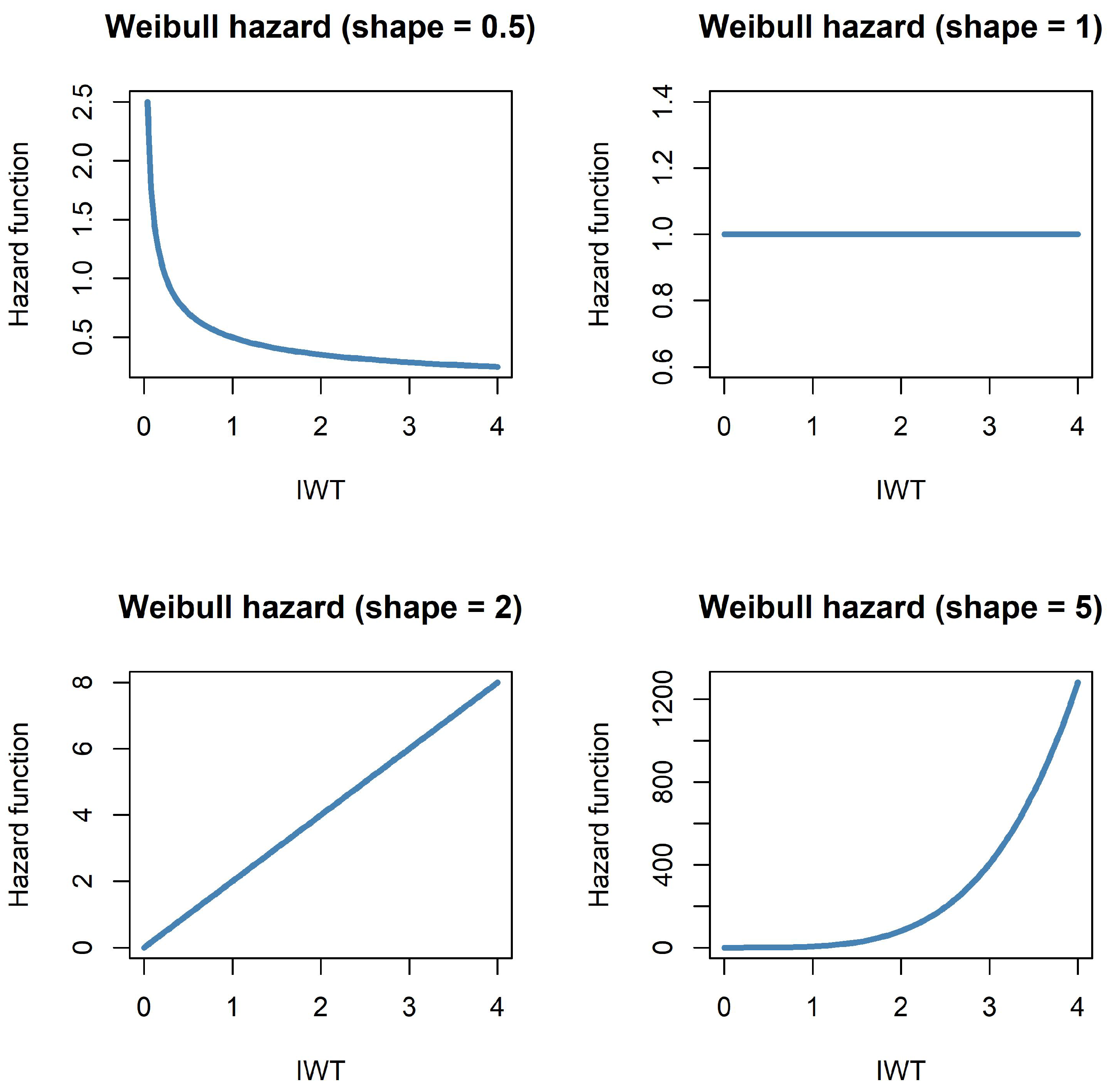
2.1.1. Weibull Counting Process

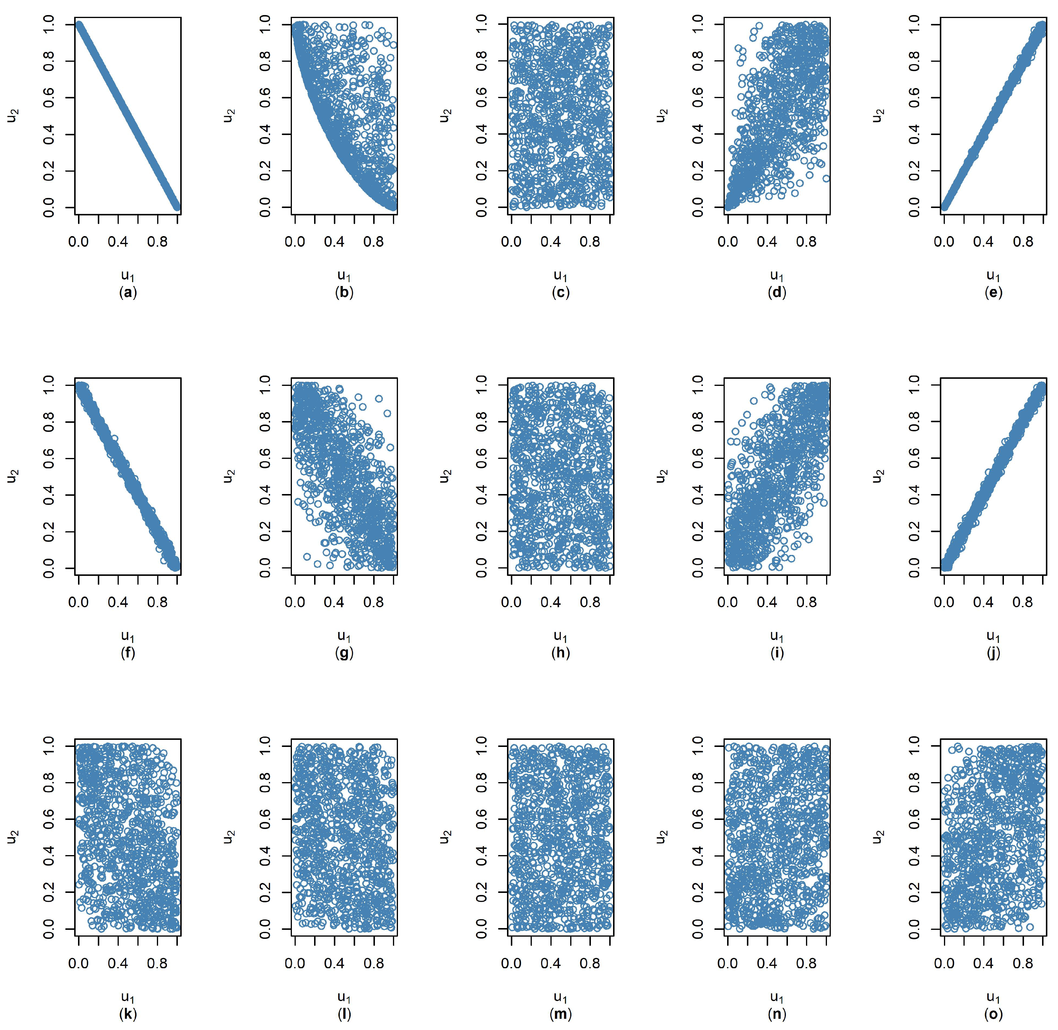
In this study, we let the counting process $\underline{N}={\left\{N\left(t\right)\right\}}_{t\ge 0}$ follow a basic Weibull counting process as in Mohd Ramli et al. (2019), whereby the corresponding continuous random variable of the inter-claim arrival time, $W_i$, is defined as:

$$\begin{array}{c}\hfill W_i=\left\{\begin{array}{cc}{T}_i\hfill & \mathrm{for}i=1\hfill \\ T_i-T_{i-1}\hfill & \mathrm{for}i=2,3,...,\hfill \end{array}\right.\end{array}$$

(2)

which follows a Weibull distribution. The time elapsed between two successive claims arrival is called the interwaiting time (henceforth IWT) of the counting process $N\left(t\right)$. Each pair of the joint variables forms a sequence of i.i.d. random vectors ${\left\{\left(X_i,W_i\right)\right\}}_{i\in N}$. The mean and variance of a Weibull count model with shape parameter $\lambda$ and scale parameter $\beta$, derived by McShane et al. (2008) are given by:

$$\begin{array}{cc}\hfill \mathrm{E}\left[N\left(t\right)\right]& ={\displaystyle \sum _{n=1}^{\infty }}{\displaystyle \sum _{j=n}^{\infty }}\frac{n{\left(-1\right)}^{j+n}{\left(t^{\lambda }/\beta \right)}^j{\tau }_j^n}{\Gamma \left(\lambda j+1\right)},\hfill \\ \hfill \mathrm{Var}\left[N\left(t\right)\right]& =\mathrm{E}\left[N^2\left(t\right)\right]-{\mathrm{E}}^2\left[N\left(t\right)\right]\hfill \end{array}$$

(3)

$$\begin{array}{cc}\hfill & ={\displaystyle \sum _{n=2}^{\infty }}{\displaystyle \sum _{j=n}^{\infty }}\frac{n^2{\left(-1\right)}^{j+n}{\left(t^{\lambda }/\beta \right)}^j{\tau }_j^n}{\Gamma \left(\lambda j+1\right)}-{\left({\displaystyle \sum _{n=1}^{\infty }}{\displaystyle \sum _{j=n}^{\infty }}\frac{n{\left(-1\right)}^{j+n}{\left(t^{\lambda }/\beta \right)}^j{\tau }_j^n}{\Gamma \left(\lambda j+1\right)}\right)}^2,\hfill \end{array}$$

(4)

where

$$\begin{array}{cc}\hfill {\tau }_j^n& =\left\{\begin{array}{cc}\frac{\Gamma \left(\lambda j+1\right)}{\Gamma \left(j+1\right)},\hfill & \mathrm{for}n=0,j=0,1,2,...\hfill \\ {\displaystyle \sum _{m=n-1}^{j-1}}{\tau }_j^{n-1}\frac{\Gamma \left(\lambda j-\lambda m+1\right)}{\Gamma \left(j-m+1\right)},\hfill & \mathrm{for}n=1,2,3,...,j=n,n+1,n+2,...,\hfill \end{array}\right.\hfill \end{array}$$

in which the parameter n denotes the number of events that occur in the interval $[0,t]$.

Although the memoryless property of the exponentially distributed IWT allows for mathematical convenience, the Poisson counting process is only adequate if the data satisfy the restrictive assumption of equidispersion in which the variance of the data is equal to their mean. Hence, the Weibull count model is a better alternative for its ability to accommodate both overdispersed and underdispersed datasets. It also nests commonly used count models, including the Poisson and the negative binomial distributions. Additionally, the Weibull count model also allows for non-constant hazard rates that vary according to the duration of the IWT (McShane et al. 2008). The hazard function characterizes the IWT distribution and relates them to the type of dispersion observed in the corresponding count data. Past studies (Jose and Abraham 2011; McShane et al. 2008; Winkelmann 1995) have verified that the underlying IWT displays negative (positive) duration dependence under a decreasing (increasing) hazard for shape parameter of 0 $<\lambda <1$ ($\lambda >1$) which causes overdispersion (underdispersion). The lack of duration dependence for $\lambda$ = 1 leads to the Poisson distribution with a constant hazard function, as shown in Figure 1.

We also note that there are two types of dependency applied when modeling the IWT under the Weibull counting process. First dependency lying between the duration of the IWT and the frequency of the claims arrival represented by non-constant hazard rates. As mentioned in McShane et al. (2008) and Winkelmann (1995), the negative (positive) duration dependence indicates a higher (lower) probability of claims occurring immediately after the occurrence of previous claims and decreases (increases) steadily as the IWT increases. This implies that the overdispersed (underdispersed) cases produce higher claims frequencies under short (long) IWT and vice versa.

2.1.2. Copula

The second dependency is between the IWT and its subsequent claims amount, which is captured by a copula. A copula provides a more convenient way to model any joint distribution of two or more random variables. We can model the marginal distributions of each variable by itself, and the copula can link these into a joint distribution. As we allow dependency between the claims size $X_i$, and the inter-arrival time $W_i$, we have a dependent Sparre–Andersen risk process with a dependence structure defined by a copula or other joint probability functions. Please note that when the marginals are negatively (positively) correlated, a large claim amount $X_i$ will occur following a short (long) inter-arrival claim time $W_i$, and vice versa. In this study, the dependence structure between the two marginals of X and W are described by a few copulae including the Clayton, Frank and FGM copulae.

Both the Clayton and Frank copulae belong to the same Archimedean family, in which the cumulative distribution function (CDF) of each copula is given by:

$$\begin{array}{c}\hfill C_{\theta }^{Clayton}\left(F_X\left(x\right),F_W\left(w\right)\right)={max\left\{{F_X\left(x\right)}^{-\theta }+{F_W\left(w\right)}^{-\theta }-1,0\right\}}^{-\frac{1}{\theta }},\end{array}$$

(5)

where $\theta \in \left[-1,\infty \right)$,

$$\begin{array}{c}\hfill C_{\theta }^{Frank}\left(F_X\left(x\right),F_W\left(w\right)\right)=-\frac{1}{\theta }ln\left(1+\frac{(e^{-\theta F_X\left(x\right)}-1)(e^{-\theta F_W\left(w\right)}-1)}{{(e}^{-\theta }-1)}\right),\end{array}$$

(6)

where $\theta \in \mathbb{R}$. The CDF of an FGM copula, which is from a different class of copula family is given by:

$$\begin{array}{cc}\hfill C_{\theta }^{FGM}\left(F_X\left(x\right),F_W\left(w\right)\right)& =F_X\left(x\right)F_W\left(w\right)+\theta \left(1-F_X\left(x\right)\right)\left(1-F_W\left(s\right)\right),\hfill \end{array}$$

(7)

where $\theta \in \left[-1,1\right]$ represents the dependence parameter (Klugman and Parsa 1999; Ly et al. 2019). The copulae return to an independence copula when $\theta =0$. The FGM copula is a popular choice in extreme value analysis and risk management (Mao and Yang 2015) due to its simplicity and analytical tractability, despite its ability to capture only moderate dependency. The moderate dependence structure for FGM copula can be seen in Figure 2k–o, in which $\theta \in \left[-1,1\right]$ is restricted to Kendall’s tau, $\tau \in \left[-2/9,2/9\right]$. In contrast, the Clayton copula (Figure 2a,e) and Frank copula (Figure 2f,j) allow for a wider range of dependency with $\tau \in \left[-1,1\right]$, as shown by the almost linear scatter plots of strong negative and positive dependency. However, the Frank copula could neither capture lower nor upper tail dependence, whereas the Clayton copula allows for lower tail dependence, or dependency on small values (Ly et al. 2019). The lower tail dependency can be seen clearly in its ’ice cream cone’ shapes as in Figure 2b,d.

2.2. Recursive Moment Expressions

The general form of the m-th moment of aggregate discounted claims $Z\left(t\right)$, as given here,

$$\begin{array}{cc}\hfill {\mu }_z^{\left(m\right)}\left(T\right)=\mathrm{E}\left[Z^m\left(T\right)\right]& ={\int }_0^T{f}_w\left(s\right)e^{-m\delta s}\mathrm{E}\left(X^m|W=s\right)ds\hfill \\ \hfill & +{\int }_0^T{f}_w\left(s\right)e^{-m\delta s}{\mu }_z^{\left(m\right)}\left(T-s\right)ds\hfill \\ \hfill & +{\displaystyle \sum _{j=1}^{m-1}}\left(\genfrac{}{}{0pt}{}{m}{j}\right){\int }_0^T{f}_w\left(s\right)e^{-m\delta s}\mathrm{E}\left(X^j|W=s\right){\mu }_z^{\left(m-j\right)}\left(T-s\right)ds,\hfill \end{array}$$

(8)

has a recursive nature (Barges et al. 2011; Mohd Ramli and Jang 2014). Working with explicit solutions of Equation (8) require heavy computational capacity due to lengthy expressions as seen in Mohd Ramli and Jang (2014) and Mohd Ramli et al. (2018). We therefore use the Monte Carlo simulation to compute the higher order of moments in a much shorter period with a common computational capacity. Hence, the mathematical properties of the insurance risk portfolio can be examined in a more efficient and viable manner despite the complicated expressions, which would be welcomed by the industrial community (Driels and Shin 2004).

2.3. Monte Carlo Simulation

Monte Carlo simulation is a popular and powerful quantitative tool often used in risk analysis such as in evaluation of insurers’ capital requirements (Casarano et al. 2017), estimation of claim size distribution (Bar-Lev and Ridder 2019), mortality projection (Zamzuri and Hui 2020) and bootstrapping approach in Structural Equation Modeling (Razak et al. 2019). We apply the Monte Carlo simulations to incorporate and understand the impact of risk and uncertainty in our model by computing the probability of different outcomes in a risk process (Zamzuri and Hui 2020).

In this study, we simulate the aggregate discounted claims process using the estimated parameters and distributions from a real insurance dataset. In simulating the copula function, we adopt the same approach as Kelly (2007), whereby the first stage involves modeling the unidimensional marginal distributions while the second stage involves modeling the dependence structure. The steps taken in the simulation process are the following:

• Generate pairs of dependent random variates $\left\{\left(X_i,W_i\right)\right\}$ from multivariate distributions constructed from the chosen copula. The multivariate distributions are based on the best-fit distribution obtained from the insurance dataset.
• Compute the random time $T_i$, from the accumulated $W_i$ as in Equation (2).
• Compute the aggregate discounted claims $Z\left(T\right)$, by assuming deterministic $\delta$.
• Stop running the iterations once the $T_i$ is above a pre-determined term of a policy contract.
• Repeat the process from step 1 to 4 for n simulations.
• Determine the moments, premium and VaR from the simulated risk process $Z\left(T\right)$.

3. Results and Discussion

In this section, we organize the results and discussion by first showing the consistency of results returned by the Monte Carlo simulation method with results obtained in previous studies (Section 3.1). Next, we fit the aggregate discounted claims model to the New Zealand catastrophe data in Section 3.2. Using the estimated parameters of the claims size distribution, the IWT distribution and the dependency between these marginals, we then examine the risk portfolio of the New Zealand catastrophe dataset. This includes computing the value of moments, premium and VaR in Section 3.3. Finally, we perform scenario analysis in Section 3.4 by varying the parameters of the Weibull process and the copulae to examine the impact on the risk portfolio.

3.1. Results Verification

We first consider the special case of a Weibull IWT with the shape parameter $\lambda =1$ to ensure consistency of the Monte Carlo simulations with the numerical values obtained through Laplace transform as in Barges et al. (2011), Mohd Ramli and Jang (2014) and Mohd Ramli et al. (2018). We simulate pairs of the joint variables of random vectors ${(X_i,W_i)}_{(i\in N)}$ with an FGM copula defining the dependency between the variables. The values were computed using the same parameters in which $X\sim$ Exp$(\alpha =0.01)$, W∼ Exp$(\beta =1)$, $\delta =0.04$ and $T=5$ for different values of $\theta$. The average number of iterations for each simulation is 5, which is consistent with the average of the exponentially distributed IWT. The process is then repeated for $n=100,000$ simulations.

The mean and variance of the aggregate discounted claims obtained via Monte Carlo simulation are presented in

Table 1. Verification of the Monte Carlo Simulation.

Moments	$\mathit{\theta }$	Monte Carlo	Laplace Transform	Relative Deviation
	−0.999	479.23	477.66	0.330%
	−0.9	474.83	475.23	0.084%
	−0.5	469.16	465.43	0.803%
Mean	0	452.79	453.17	0.084%
	0.5	440.59	440.92	0.074%
	0.9	433.43	431.12	0.537%
	0.999	430.23	428.69	0.359%
	−0.999	106,554.00	106,351.84	0.190%
	−0.9	105,554.20	103,929.50	1.563%
	−0.5	94,099.89	94,253.78	0.163%
Variance	0	80,630.85	82,420.23	2.171%
	0.5	69,601.11	70,874.44	1.797%
	0.9	61,217.14	61,845.86	1.017%
	0.999	59.182.13	59,638.74	0.766%

and we compare the results with the explicit solution under the Laplace transform as in Mohd Ramli et al. (2018). The simulation results show only slight deviation from the values computed using the Laplace transform, of less than 1% differences for the mean and $2\%$ for the variance.

3.2. Fitting Distribution and Parameter Estimation of Insurance Datasets

In this section, we fit the aggregate discounted claim models on the New Zealand catastrophe occurrences and losses amount data from 1968 to 2014 which was retrieved from the CASdatasets package in R Statistical Software (Dutang and Charpentier 2020). We estimate the parameters of the fitted distributions of the claims size and the IWT, as well as the dependency between the marginals, using the maximum likelihood estimation method.

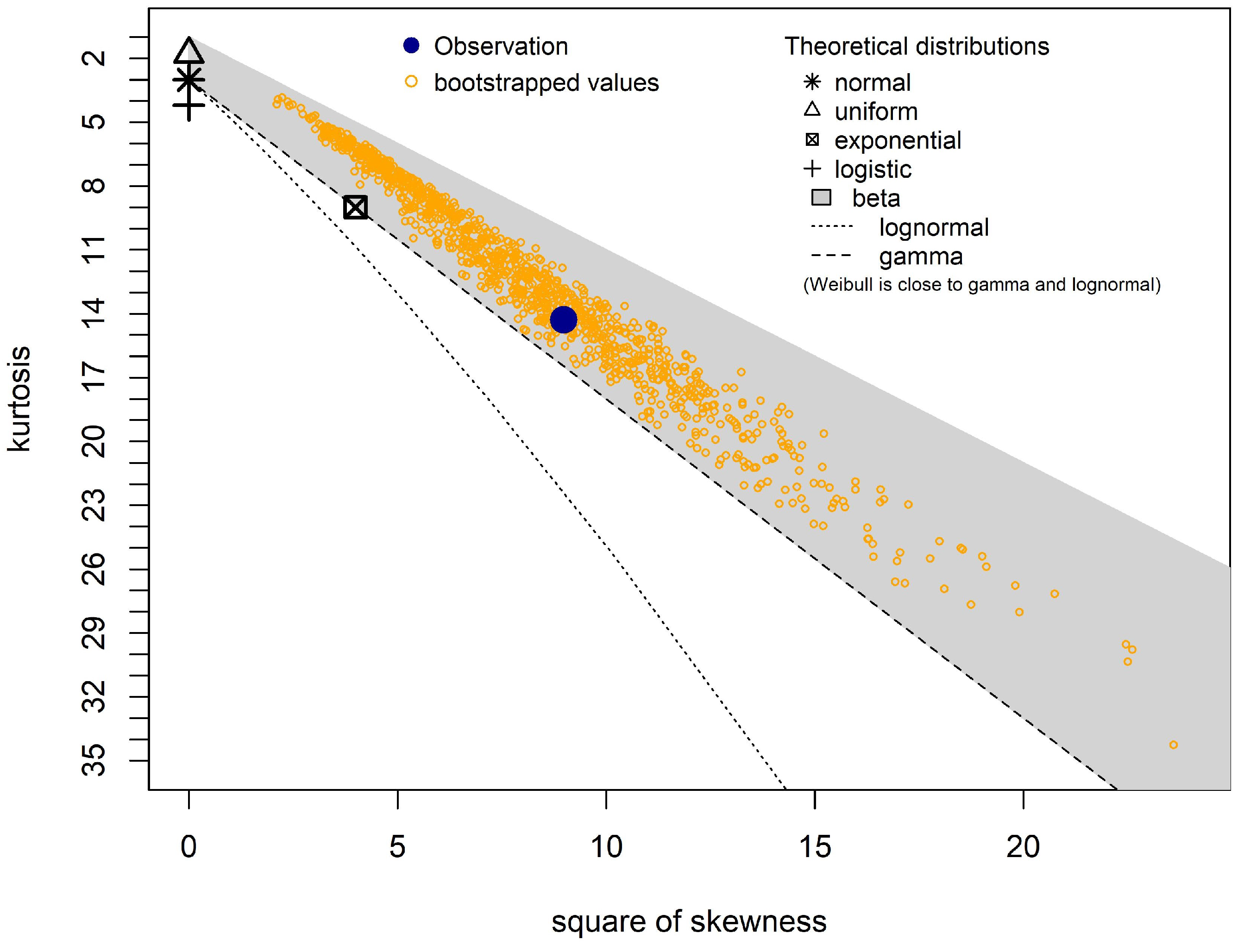
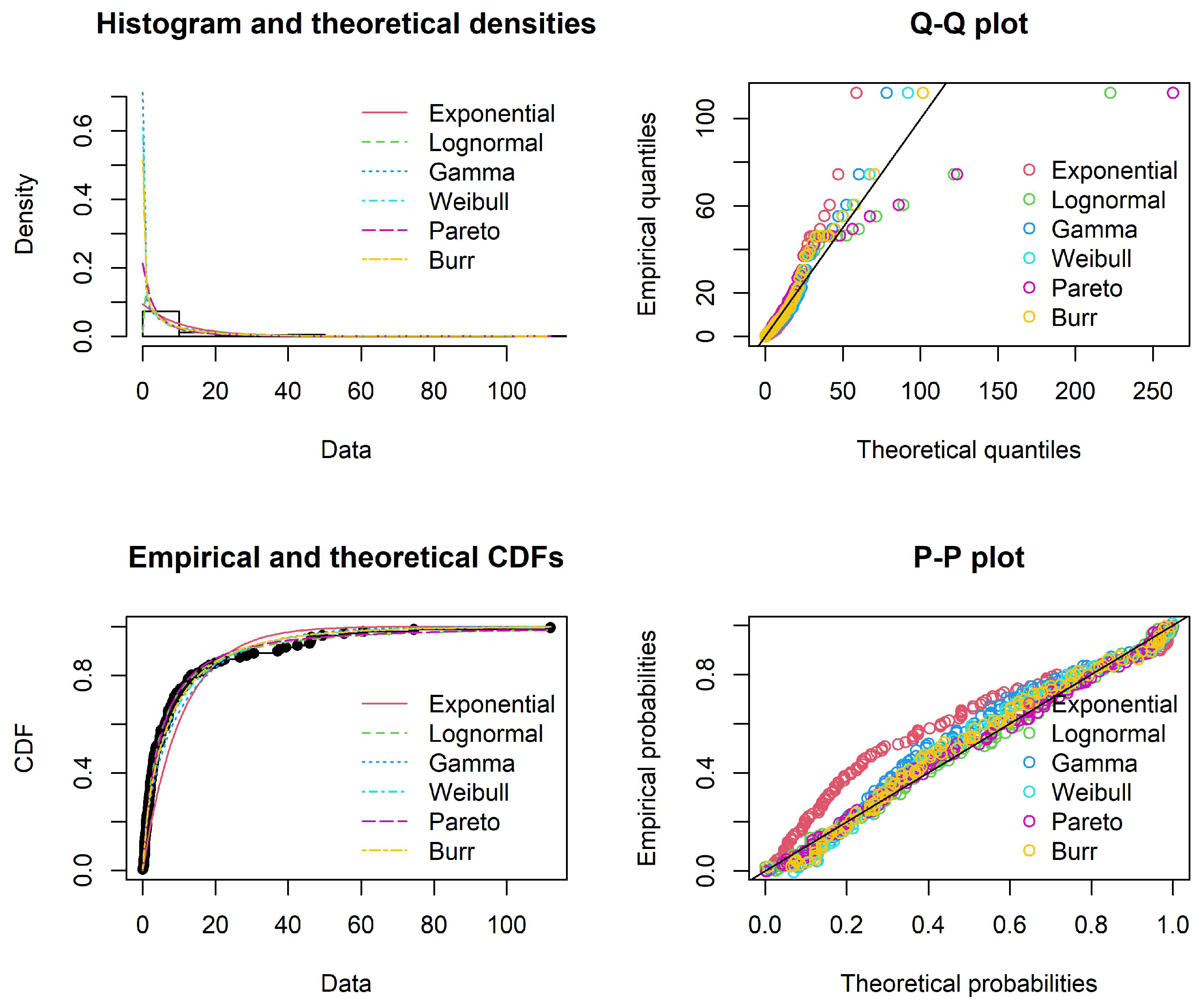
3.2.1. The Claim Sizes Distribution

The Cullen and Frey (Cullen et al. 1999) graph in Figure 3 illustrates the skewness-kurtosis plot of the empirical distribution of the New Zealand catastrophe loss claims. The values are computed on 1000 bootstrap samples to allow for the uncertainty of the estimated values of kurtosis and skewness from data. This graph exhibits some common distributions on the plot to help with the choice of distributions to fit to data. The normal, uniform, and logistic distributions are not good fits for the data since the skewness-kurtosis points of the distribution are far from the empirical value. The descriptive statistic in

Table 2. Descriptive statistics for New Zealand catastrophe claims sizes.

Min	Max	Median	Mean	Estimated Std Dev	Estimated Skewness	Estimated Kurtosis
0.01	112	3.6	10.67252	17.14509	2.997792	14.29496

shows a positive skewness and a heavy-tailed kurtosis. Thus, the fit of three common right-skewed distributions could be considered, which are the Weibull, Gamma and Lognormal distributions, together with other heavy-tailed distributions such as Pareto and Burr. The results in

Table 3. Goodness-of-fit (GOF) measures for fitted distributions on the claim sizes.

	GOF Criterion			GOF Test
Distribution	−2 Log Likelihood	AIC	BIC	KS Test (p-Value)	AD Test (p-Value)
Exponential	828.447	830.447	833.260	0.0000	0.0000
Lognormal	787.928	791.928	797.552	0.9980	0.9775
Gamma	804.195	808.195	813.820	0.0912	0.0389
Weibull	796.037	800.037	805.662	0.4291	0.1797
Pareto	788.541	792.541	798.165	0.9096	0.8201
Burr	788.420	794.421	802.857	0.9339	0.8521

and Figure 4 show that the lognormal distribution, with a meanlog of 1.35969 and an sdlog of 1.52856, provides the best fit for the claims size distribution (values in million USD). The fitted lognormal distribution has the lowest negative log likelihood, Akaike information criterion (AIC) and Bayesian information criterion (BIC) values, with significant p-values under the Kolmogorov–Smirnov (KS) and Anderson-Darling (AD) test.

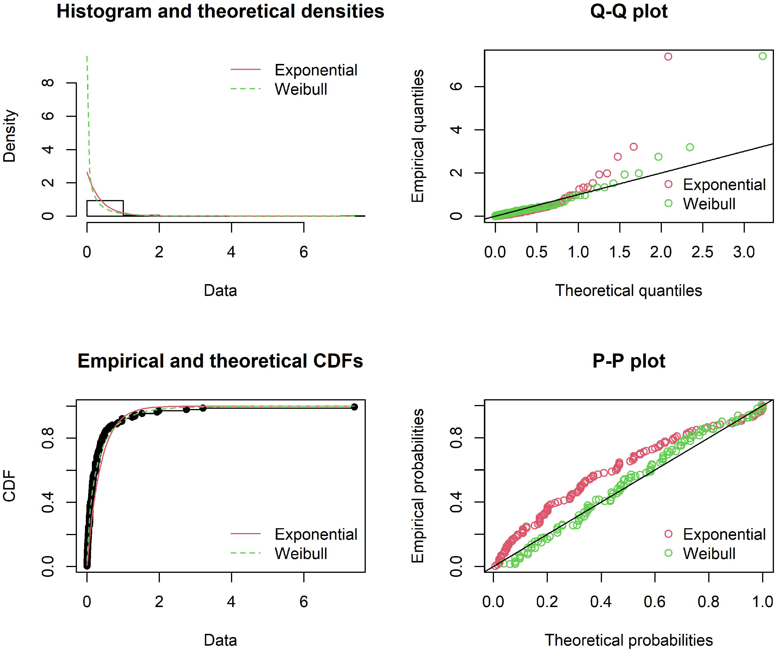
3.2.2. The Interwaiting Time Distribution

The descriptive statistics of the IWT of the New Zealand catastrophe claims arrival in

Table 4. Descriptive statistics for the IWT (in years) of claims arrival.

Min	Max	Median	Mean	Estimated Std Dev	Estimated Skewness	Estimated Kurtosis
0.0027	7.3922	0.1478	0.3786	0.8125	6.0819	49.9694

imply that the claims arrive on average every 138.29 days, with a maximum IWT of 7.39 years. The IWT exhibits positive skewness with high kurtosis.

Table 5. Goodness-of-fit (GOF) measures for fitted distributions on the IWT.

		GOF Criterion		GOF Test
Distribution	Estimated Parameters	AIC	BIC	KS Test (p-Value)	AD Test (p-Value)
Weibull	$\lambda$ = 0.700152 $\beta$ = 0.282022	−27.4824	−21.8580	0.5383	0.2877
Exponential	$\alpha$ = 2.641138	9.08241	11.8946	0.0001	0.0000

and Figure 5 show that the Weibull distribution is the best fit for the IWT when compared with exponential distribution. The Weibull shape parameter value of 0.700152 < 1 indicates an overdispersed claims occurrences, implying that the claims arrive at times that vary more than expected.

3.2.3. The Dependency between the Claim Sizes and the IWT

Table 6. Goodness-of-fit criterion for fitted copula on the dependency between the claim sizes and the IWT.

Copula	Estimated Parameter, $\mathit{\theta }$	Log Likelihood	AIC	BIC
Independence	0	0	0	0
Gaussian	0.19	2.02	−2.04	0.77
T	0.19	2.12	−0.25	5.38
Clayton	0.32	3.57	−5.13	−2.32
Gumbel	1.09	0.92	0.17	2.98
Frank	1.1	1.91	−1.81	1
Joe	1.06	0.17	1.65	4.47

exhibits that the Clayton copula is the best fit for the dependence structure between the IWT and its subsequent claim amount embedded in the New Zealand catastrophe historical data. Since Clayton copula allows for lower tail dependence, this indicates that the IWT and the subsequent claims amount show more dependency on small values. The positive dependency between the marginals as shown by parameter $\theta =0.32$ or the equivalent Kendall’s $\tau$ of 0.14, implies that the large (small) claim amount would occur following the long (short) IWT.

3.3. Risk Characteristic of the Risk Process with Overdispersed Claim Arrival

We will examine the effect of overdispersion in the claims arrival of the New Zealand catastrophe historical data on the moments, premium and VaR in comparison to the equidispersed counting process through the Monte Carlo simulation. We are setting $\delta =0.025$, $X_i\sim$lognormal (1.3597,1.5286), with $W_i$ following the Weibull and exponential distributions from the estimated parameters as in Table 5. The dependency of $X_i$ and $W_i$ is captured through a Clayton copula with $\theta =0.32$.

The simulation results as illustrated in

Table 7. Simulated moments of the New Zealand catastrophe risk process for T = 5.

IWT Distribution	Mean	Variance	Skewness	Kurtosis
Weibull	169.343	21313.540	6.296	145.444
Exponential	154.034	18239.790	7.242	150.931

show that both risk processes of $Z\left(t\right)$ are a right-skewed distribution based on the positive skewness. The high value of kurtosis from the results indicates a heavy-tailed distribution. However, the exponential IWT underestimates the value of the mean and variance, which results in a lower value of premium and VaR compared with the overdispersed Weibull IWT as seen in

Table 8. Simulated VaR and premium of the New Zealand catastrophic risk process for T = 5.

IWT	VaR ($m)		Premium Amount ($m)
Distribution	95%	99.50%	Mean Principle	Std Dev Principle
Weibull	406.757	846.901	186.278	183.942
Exponential	363.706	809.141	169.438	167.540

.

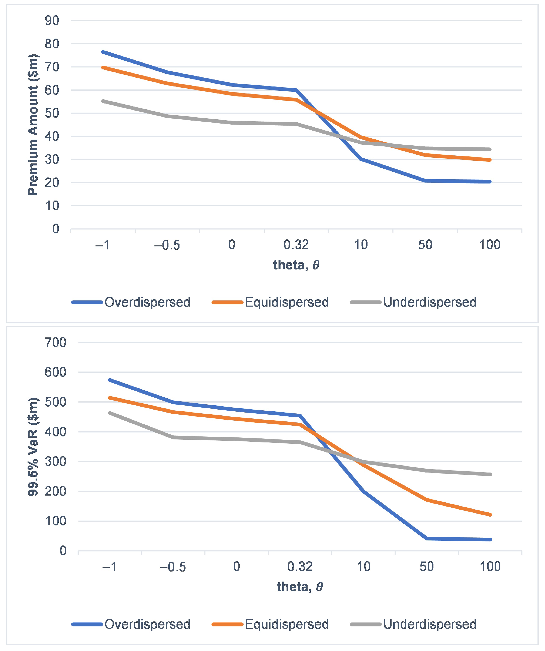
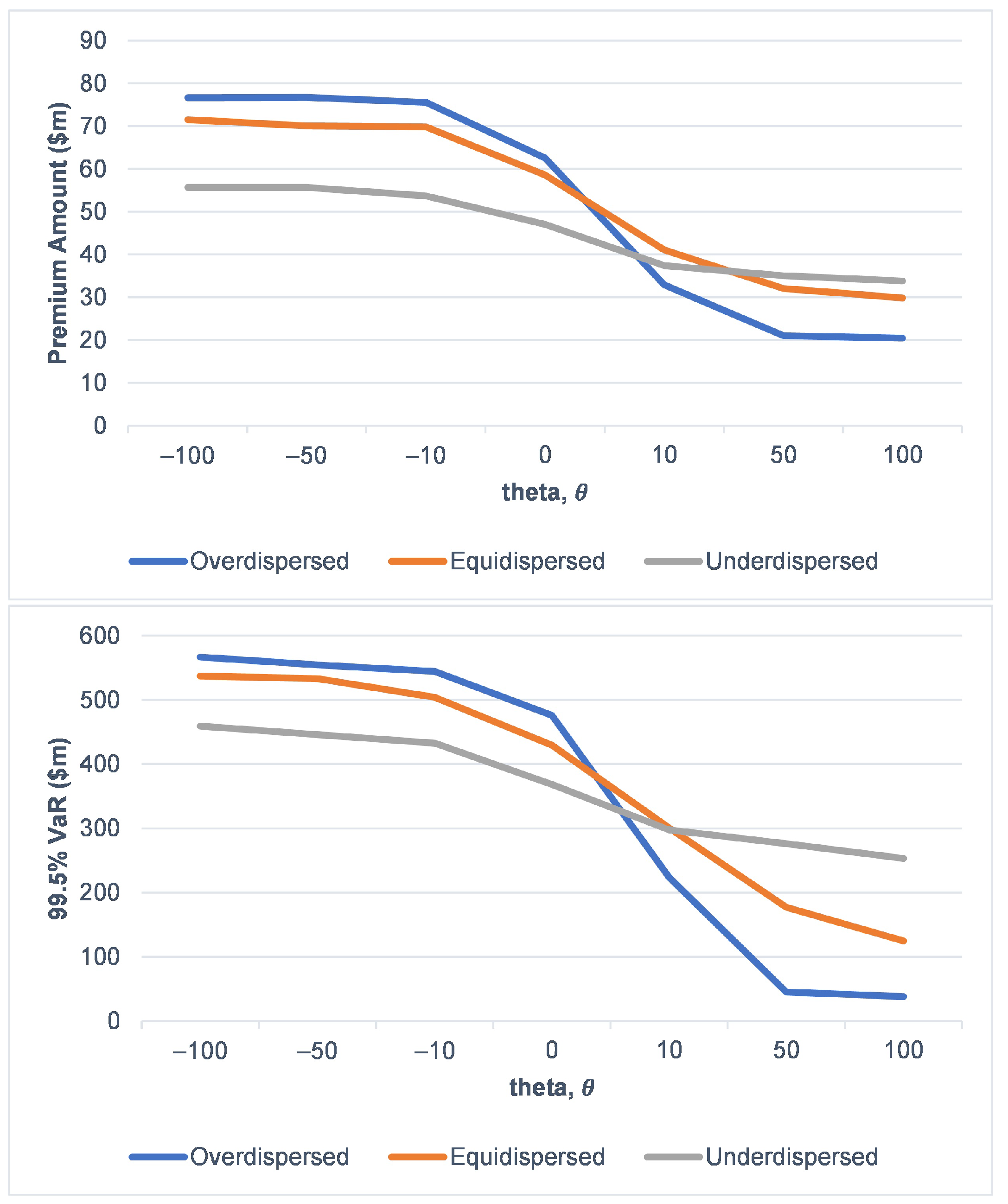
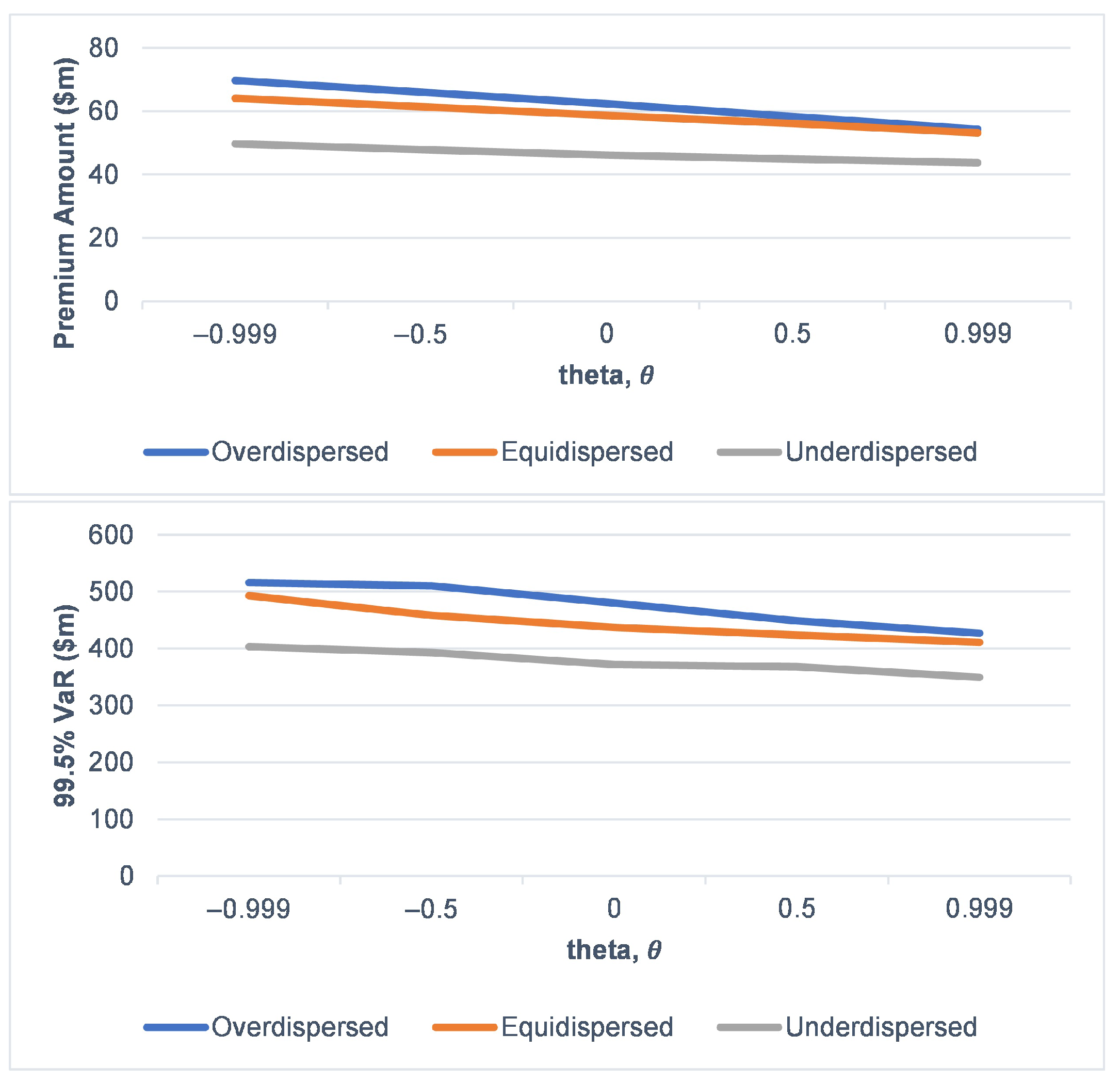
3.4. Scenario Analysis on Risk Characteristic of the Risk Process under Various Dispersion Effect on Claims Arrival

In this section, we perform a scenario analysis on the moments, premium and VaR by varying the shape $\lambda$ and the scale $\beta$ parameters under the Weibull IWT distribution. This is done to allow for various dispersion effect of claims occurrences, across different dependence parameter $\theta$. The parameters of the Weibull count process are chosen so that they have an equal mean of claim frequencies but with different variances, obtained through Equation (4).

Table 9. Marginal mean and variance of overdispersed, equidispersed and underdispersed Weibull count models, ${\mathrm{Weibull}}_C$ when T = 5.

	Overdispersed	Equidispersed	Underdispersed
	${\mathbf{Weibull}}_{\mathit{C}}$ ($\mathit{\lambda }=0.5,\mathit{\beta }=0.945$)	${\mathbf{Weibull}}_{\mathit{C}}$ ($\mathit{\lambda }=1,\mathit{\beta }=1.17835$)	${\mathbf{Weibull}}_{\mathit{C}}$ ($\mathit{\lambda }=2,\mathit{\beta }=1.5$)
Mean	4.243	4.243	4.243
Variance	9.903	4.243	1.375

illustrates the chosen parameter in which the equidispersed case has an equal mean and variance of 4.243, whereas the variance under the overdispersed (underdispersed) case is higher (lower) than the mean. This is then reflected in the probability distribution of the claims frequencies as seen in Figure 6. There is an increased chance of more claims occurring under the overdispersed case, while the claim frequencies are more concentrated around the mean for the underdispersed case in a fixed time interval.

Please note that the simulation of the aggregate discounted claims under Weibull process adopt two types of dependency. The first type is the duration dependence between the duration of the IWT, $W_i$, and the frequency of claims arrivals, which causes dispersed dataset. The second type is the dependency between the $W_i$ and its subsequent claims amount $X_i$, which is captured by a dependence parameter $\theta$ of a copula.

Table 10. Simulated moments under various dispersion of claims occurrences across different $\theta$ under a Clayton copula when T = 5.

	Overdispersed ${\mathbf{Weibull}}_{\mathit{C}}(\mathit{\lambda }=0.5,\mathit{\beta }=0.945)$
$\mathit{\theta }$	Mean	Variance	Skewness	Kurtosis
−1	66.359	10202.750	9.423	276.883
−0.5	58.933	7595.139	7.010	128.587
0	53.764	7168.824	10.130	294.856
0.32	51.266	7538.556	22.392	1599.203
10	26.722	1205.303	16.188	714.862
50	19.757	109.521	2.620	105.380
100	19.454	90.367	−0.336	−0.839
	Equidispersed ${\mathrm{Weibull}}_{\mathbf{C}}(\mathbf{\lambda }=\mathbf{1},\mathbf{\beta }=\mathbf{1.17835})$
$\mathbf{\theta }$	Mean	Variance	Skewness	Kurtosis
−1	60.663	8240.178	7.779	162.108
−0.5	54.657	6749.611	8.895	190.364
0	50.751	5835.950	10.186	315.298
0.32	48.389	5557.512	13.696	576.241
10	34.768	2378.918	13.	372.840
50	28.978	855.983	21.968	1236.261
100	27.540	533.322	25.754	1589.694
	Underdispersed ${\mathrm{Weibull}}_{\mathbf{C}}(\mathbf{\lambda }=\mathbf{2},\mathbf{\beta }=\mathbf{1.5})$
$\mathbf{\theta }$	Mean	Variance	Skewness	Kurtosis
−1	47.414	6147.893	8.180	148.807
−0.5	42.014	4487.100	11.205	347.476
0	39.587	3991.358	9.331	190.339
0.32	38.672	4477.052	13.927	431.441
10	32.096	2714.674	14.606	497.202
50	30.036	2288.304	22.567	1324.124
100	29.623	2289.057	25.280	1591.957

shows that the highest mean and variance are obtained when the $X_i$ and $W_i$ exhibit strong negative correlation as seen when $\theta =-1$. This is intuitively reasonable; short IWT (or frequent claim occurrence) followed by large claims amount $X_i$, will produce higher value of moments. However, as $\theta$ changes from negative to positive dependency, the mean and variance are decreasing under all dispersion scenarios.

In comparison to an equidispersed process, the case of overdispersed claims occurrences produces the highest first two moments when $\theta$ is negative. Conversely, the underdispersed case shows the highest values of moments when $\theta$ is positive. These outcomes could be related to both aforementioned types of dependencies under Weibull process. Higher claim frequencies under short (long) IWT will result in many large claims when $\theta$ is negative (positive).

Additionally, the positive skewness and the high value of kurtosis imply that the risk process exhibits a right-skewed with a heavy-tailed risk distribution. However, as $\theta$ changes to a strong positive dependency, the tail of the risk process under the overdispersed (underdispersed) case is less (more) skewed with less (more) extreme values on the tail distribution as shown in the value for skewness and kurtosis. This is then reflected in

Table 11. Simulated VaR and premium ($\kappa =0.1$) under various dispersion of claims occurrences across different $\theta$ under a Clayton copula when T = 5.

	Overdispersed ${\mathbf{Weibull}}_{\mathit{C}}(\mathit{\lambda }=0.5,\mathit{\beta }=0.945)$
$\mathit{\theta }$	VaR ($m)		Premium Amount ($m)
	95%	99.50%	Mean Principle	Std Dev Principle
−1	225.744	573.577	72.994	76.459
−0.5	197.729	498.658	64.827	67.649
0	180.155	473.747	59.140	62.231
0.32	167.568	454.264	56.392	59.948
10	63.731	199.876	29.394	30.194
50	34.147	41.335	21.733	20.804
100	32.855	37.793	21.399	20.405
	Equidispersed ${\mathrm{Weibull}}_{\mathbf{C}}(\mathbf{\lambda }=\mathbf{1},\mathbf{\beta }=\mathbf{1.17835})$
$\mathbf{\theta }$	VaR ($m)		Premium Amount ($m)
	95%	99.50%	Mean Principle	Std Dev Principle
−1	202.152	514.118	66.729	69.741
−0.5	176.053	466.067	60.122	62.872
0	161.369	443.094	55.827	58.391
0.32	151.449	424.326	53.228	55.844
10	88.749	288.379	38.245	39.646
50	58.319	170.823	31.876	31.904
100	52.508	120.991	30.293	29.849
	Equidispersed ${\mathrm{Weibull}}_{\mathbf{C}}(\mathbf{\lambda }=\mathbf{2},\mathbf{\beta }=\mathbf{1.5})$
$\mathbf{\theta }$	VaR ($m)		Premium Amount ($m)
	95%	99.50%	Mean Principle	Std Dev Principle
−1	163.186	463.176	52.155	55.254
−0.5	138.329	380.708	46.215	48.712
0	128.152	374.841	43.546	45.905
0.32	121.294	364.802	42.540	45.363
10	91.612	298.824	35.306	37.307
50	80.044	269.078	33.039	34.819
100	77.195	256.812	32.585	34.407

, whereby the risk process with heavier-tailed distribution leads to a greater difference between the value of 95% and the 99.5% VaR. The 99.5% VaR has more than tripled in value than the 95% VaR under the most heavy-tailed risk process shown by the underdispersed case with a strong positive $\theta$.

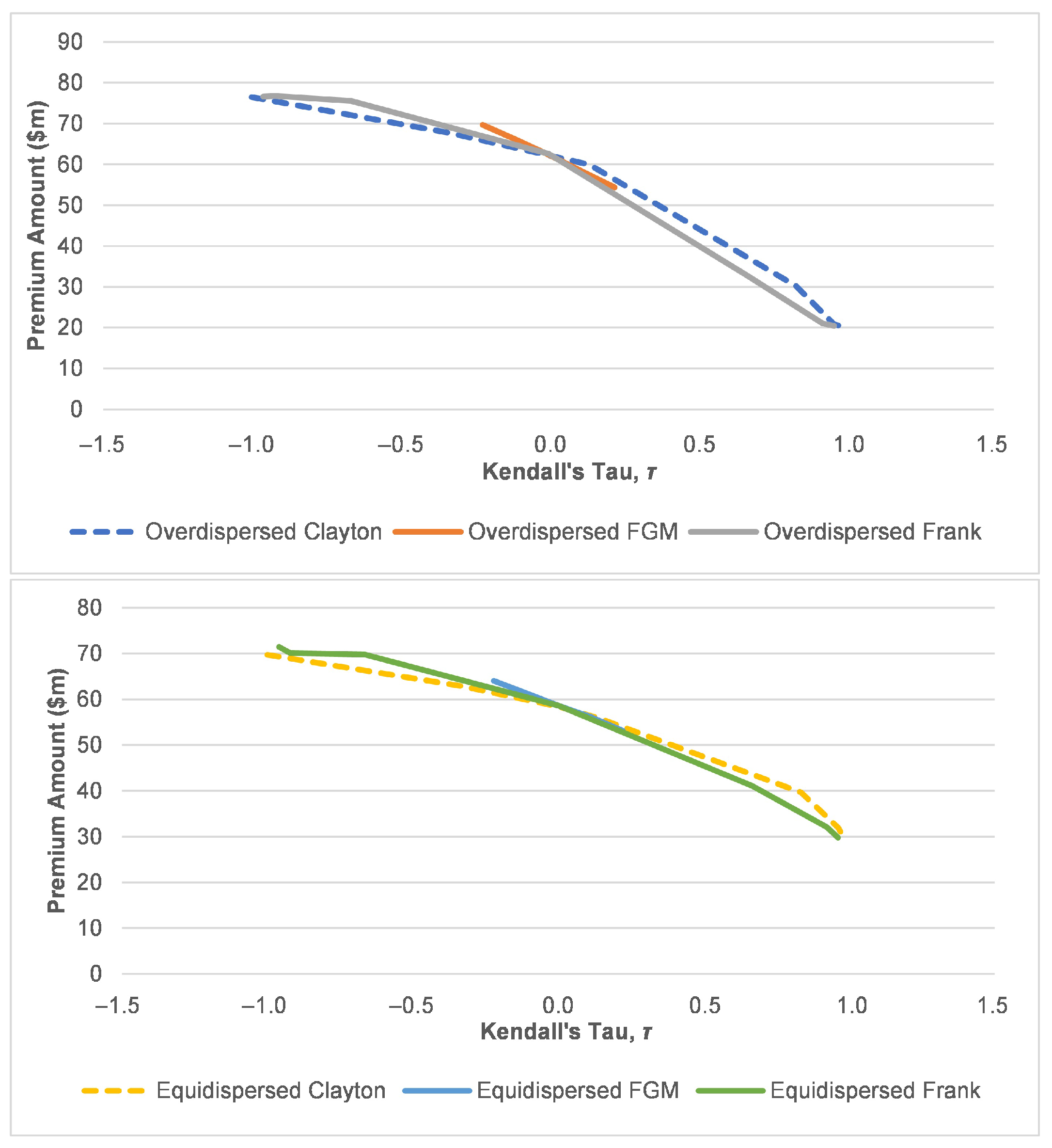
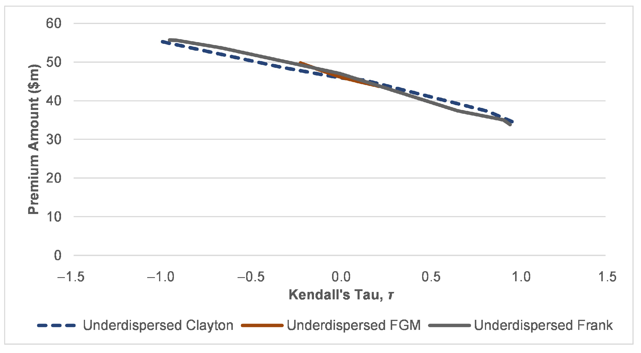
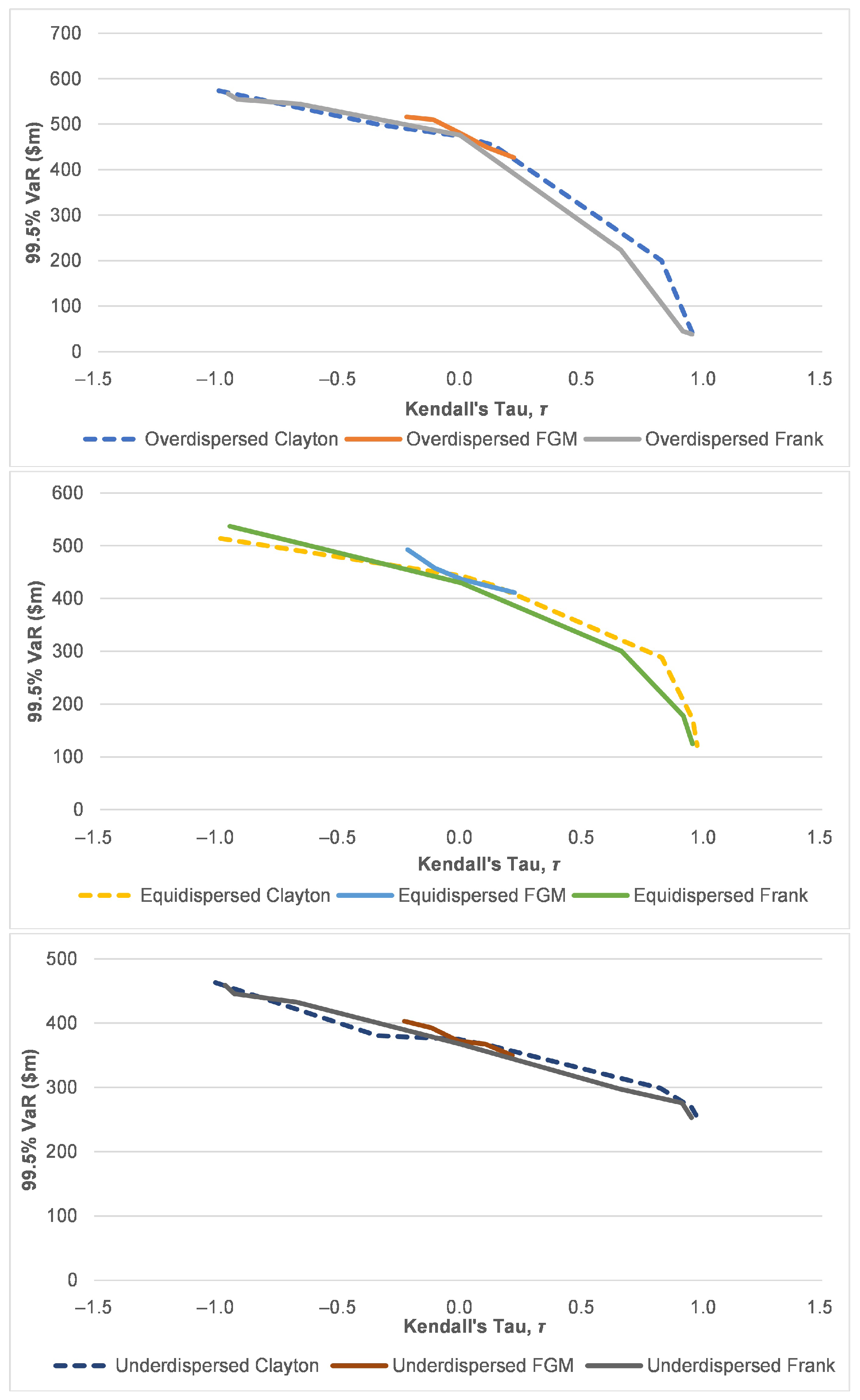
Premium Computation and VaR of the Risk Portfolio

The solvency capital requirement (SCR), which is the additional amount of funds an insurer is required to hold, should correspond to the 99.5% VaR as outlined under the Solvency II regime (Christiansen and Niemeyer 2014). In doing so, the premium should be charged appropriately, taking into account risks related to the claims experience. The computation of loaded premium, $\Pi$ according to the mean and standard deviation premium principle are given by the following:

$$\begin{array}{c}\hfill \Pi \left(T\right)=\mathrm{E}\left[Z\left(T\right)\right]+\kappa \mathrm{E}\left[Z\left(T\right)\right]\end{array}$$

(9)

$$\begin{array}{c}\hfill \Pi \left(T\right)=\mathrm{E}\left[Z\left(T\right)\right]+\kappa \sqrt{\mathrm{Var}\left[Z\left(T\right)\right]}.\end{array}$$

(10)

with $\kappa \in [0,1]$ as the loading factor.

The results presented in Table 11 and Figure 7 show that an insurer needs to charge higher premiums and set aside more capital requirement if the claims experience exhibits overdispersion (underdispersion) with negative (positive) $\theta$, in comparison to equidispersed claims experience. These results are consistent with a Frank copula which is seen in

Table 12. Simulated VaR and premium ($\kappa =0.1$) under various dispersion of claims occurrences across different $\theta$ under a Frank copula when T = 5.

	Overdispersed ${\mathbf{Weibull}}_{\mathit{C}}(\mathit{\lambda }=0.5,\mathit{\beta }=0.945)$
$\mathit{\theta }$	VaR ($m)		Premium Amount ($m)
	95%	99.50%	Mean Principle	Std Dev Principle
−100	225.816	566.751	73.363	76.605
−50	227.023	554.466	73.356	76.737
−10	222.041	544.253	72.451	75.522
0	179.770	475.843	59.577	62.559
10	74.381	223.736	31.722	32.858
50	34.979	45.038	21.940	21.018
100	33.045	38.072	21.427	20.435
	Equidispersed ${\mathrm{Weibull}}_{\mathbf{C}}(\mathbf{\lambda }=\mathbf{1},\mathbf{\beta }=\mathbf{1.17835})$
$\mathbf{\theta }$	VaR ($m)		Premium Amount ($m)
	95%	99.50%	Mean Principle	Std Dev Principle
−100	203.215	536.925	67.420	71.469
−50	204.435	532.854	67.100	70.079
−10	200.478	504.214	66.215	69.807
0	161.197	429.608	55.876	58.620
10	94.393	300.319	39.512	41.085
50	58.900	177.422	31.990	32.082
100	52.942	124.696	30.383	29.798
	Underdispersed ${\mathrm{Weibull}}_{\mathbf{C}}(\mathbf{\lambda }=\mathbf{2},\mathbf{\beta }=\mathbf{1.5})$
$\mathbf{\theta }$	VaR ($m)		Premium Amount ($m)
	95%	99.50%	Mean Principle	Std Dev Principle
−100	162.916	459.141	52.387	55.664
−50	161.985	445.691	52.355	55.655
−10	153.385	432.808	50.560	53.662
0	128.944	368.501	44.232	47.049
10	92.540	297.590	35.405	37.388
50	81.145	275.849	33.254	35.059
100	77.572	252.967	32.445	33.838

and Figure 8. However, the claims modeling based on FGM copula as represented in

Table 13. Simulated VaR and premium ($\kappa =0.1$) under various dispersion of claims occurrences across different $\theta$ under a FGM copula when T = 5.

	Overdispersed ${\mathbf{Weibull}}_{\mathit{C}}(\mathit{\lambda }=0.5,\mathit{\beta }=0.945)$
$\mathit{\theta }$	VaR ($m)		Premium Amount ($m)
	95%	99.50%	Mean Principle	Std Dev Principle
−0.999	204.390	515.814	66.564	69.693
−0.5	190.822	509.914	62.891	66.048
0	178.699	480.092	59.106	62.356
0.5	165.488	448.837	55.451	58.282
0.999	154.182	426.935	51.789	54.361
	Equidispersed ${\mathrm{Weibull}}_{\mathbf{C}}(\mathbf{\lambda }=\mathbf{1},\mathbf{\beta }=\mathbf{1.17835})$
$\mathbf{\theta }$	VaR ($m)		Premium Amount ($m)
	95%	99.50%	Mean Principle	Std Dev Principle
−0.999	178.922	492.664	60.988	64.017
−0.5	172.109	458.163	58.608	61.381
0	161.823	436.838	56.028	58.640
0.5	151.357	423.809	53.247	56.144
0.999	140.298	411.168	50.556	53.115
	Underdispersed ${\mathrm{Weibull}}_{\mathbf{C}}(\mathbf{\lambda }=\mathbf{2},\mathbf{\beta }=\mathbf{1.5})$
$\mathbf{\theta }$	VaR ($m)		Premium Amount ($m)
	95%	99.50%	Mean Principle	Std Dev Principle
−0.999	140.496	403.169	46.940	49.749
−0.5	133.912	392.826	45.231	47.897
0	126.499	372.115	43.538	46.174
0.5	120.662	367.651	42.261	44.904
0.999	115.166	349.602	40.982	43.725

and Figure 9, do not produce the same pattern because of that copula’s weak dependence structure as compared with the other two Archimedean copulae with greater dependency.

We plotted again the simulated premium and VaR across different Kendall’s $\tau$ to standardize the value on x-axis for comparison. The VaR and premium for each dispersion case exhibit the same value, respectively when $\tau =0$ as seen in Figure 10 and Figure 11. As $\tau$ changes from −1 to 1, the overdispersed (underdispersed) case illustrates the widest (narrowest) spread of values among all. On average, Frank (Clayton) copula illustrates higher value of premiums and VaR than the Clayton (Frank) copula when $\tau$ is negative (positive), while the values under FGM copula are illustrated between the two copulae.

In comparison to Mohd Ramli et al. (2019) which only illustrated the computations of the first two moments of a Weibull risk process with $\lambda =2$ under an FGM copula, we used the Monte Carlo simulation technique and obtained the higher-order moments of the Weibull risk process with wider choice of copulae. With the additional information on the asymmetry and the tail distribution of the aggregate discounted claims, insurance providers can allow for the dispersion in the claims occurrences and dependency between variables when estimating the premium and capital requirement for an insurance risk portfolio.

4. Conclusions

The ability of an insurance firm to manage surplus effectively is important to ensure capital adequacy, as required by the Solvency II standard. To allow for dispersed datasets, we propose the Weibull counting process to represent the claims arrival process of an insurance risk portfolio and an arbitrary continuous claims size. Under this model, two types of dependency were accommodated which were captured by the hazard function and the copula. We then fit the model to the historical data of New Zealand catastrophe events occurrences and losses, which was best represented by an overdispersed Weibull process with claim amounts following a lognormal distribution and a Clayton copula with a weak dependency. The moments estimation via Monte Carlo simulations shows the highest mean and variance of the aggregate discounted claims were obtained under an overdispersed claim arrivals with a strong negative correlation. The positive skewness and the high value of kurtosis of the aggregate discounted claims with Weibull IWT also implied an asymmetric and a heavy-tailed risk distribution. The scenario analysis conducted indicated that insurers will need to charge higher premiums and set aside more capital requirements as the claims experience exhibits overdispersed (underdispersed) IWT with negative (positive) dependency captured by copulae, in comparison to claims experience with equidispersed IWT. Other than computing the respective ruin probability under the Weibull risk process and applying commonly used copulae in finance and insurance, we may also examine the applicability of the model on a random annuity plan with random payments being paid at random times.

References

1. Albrecher, Hansjörg, Corina Constantinescu, and Stéphane Loisel. 2011. Explicit ruin formulas for models with dependence among risks. Insurance: Mathematics and Economics 48: 265–70. [Google Scholar] [CrossRef] [Green Version]
2. Bar-Lev, Shaul, and Ad Ridder. 2019. Monte Carlo methods for insurance risk computation. International Journal of Statistics and Probability 8: 54–74. [Google Scholar] [CrossRef]
3. Barges, Mathieu, Hélene Cossette, Stéphane Loisel, and Etienne Marceau. 2011. On the moments of aggregate discounted claims with dependence introduced by a FGM copula. ASTIN Bulletin: The Journal of the IAA 41: 215–38. [Google Scholar]
4. Boshnakov, Georgi, Tarak Kharrat, and Ian G. McHale. 2017. A bivariate Weibull count model for forecasting association football scores. International Journal of Forecasting 33: 458–66. [Google Scholar] [CrossRef] [Green Version]
5. Casarano, Giuseppe, Gilberto Castellani, Luca Passalacqua, Francesca Perla, and Paolo Zanetti. 2017. Relevant applications of Monte Carlo simulation in Solvency II. Soft Computing 21: 1181–92. [Google Scholar] [CrossRef]
6. Christiansen, Marcus C., and Andreas Niemeyer. 2014. Fundamental definition of the solvency capital requirement in Solvency II. Astin Bulletin 44: 501–33. [Google Scholar] [CrossRef] [Green Version]
7. Cullen, Alison C., H. Christopher Frey, and Christopher H. Frey. 1999. Probabilistic Techniques in Exposure Assessment: A Handbook for Dealing with Variability and Uncertainty in Models and Inputs. Berlin: Springer Science & Business Media. [Google Scholar]
8. Driels, Morris R., and Young S. Shin. 2004. Determining the Number of Iterations for Monte Carlo Simulations of Weapon Effectiveness. Technical Report. Monterey: Naval Postgraduate School Monterey. [Google Scholar]
9. Dutang, Christophe, and Arthur Charpentier. 2020. CASdatasets: Insurance Datasets. R Package Version 1.0-11. Vienna: R Core Team. [Google Scholar]
10. Hasumi, Tomohiro, Takuma Akimoto, and Yoji Aizawa. 2009. The Weibull–log Weibull distribution for inter-occurrence times of earthquakes. Physica A: Statistical Mechanics and Its Applications 388: 491–98. [Google Scholar] [CrossRef] [Green Version]
11. Jang, Jiwook. 2004. Martingale approach for moments of discounted aggregate claims. Journal of Risk and Insurance 71: 201–11. [Google Scholar] [CrossRef]
12. Jose, Kanichukattu K., and Bindu Abraham. 2011. A count model based on Mittag-Leffler interarrival times. Statistica 71: 501–14. [Google Scholar]
13. Kelly, Dana L. 2007. Using copulas to model dependence in simulation risk assessment. Paper presented at the ASME 2007 International Mechanical Engineering Congress and Exposition, Seattle, WA, USA, November 11–15; vol. 43084, pp. 81–89. [Google Scholar]
14. Klugman, Stuart A., and Rahul Parsa. 1999. Fitting bivariate loss distributions with copulas. Insurance: Mathematics and Economics 24: 139–48. [Google Scholar] [CrossRef]
15. Kreer, Markus, Ayşe Kızılersü, Anthony W. Thomas, and Alfredo D Egídio dos Reis. 2015. Goodness-of-fit tests and applications for left-truncated Weibull distributions to non-life insurance. European Actuarial Journal 5: 139–63. [Google Scholar] [CrossRef]
16. Léveillé, Ghislain, and Jose Garrido. 2001a. Moments of compound renewal sums with discounted claims. Insurance: Mathematics and Economics 28: 217–31. [Google Scholar]
17. Léveillé, Ghislain, and José Garrido. 2001b. Recursive moments of compound renewal sums with discounted claims. Scandinavian Actuarial Journal 2001: 98–110. [Google Scholar] [CrossRef]
18. Li, Shuanming, and Yi Lu. 2018. On the moments and the distribution of aggregate discounted claims in a Markovian environment. Risks 6: 59. [Google Scholar] [CrossRef] [Green Version]
19. Liu, Hanlin. 2019. Reliability and maintenance modeling for competing risk processes with Weibull inter-arrival shocks. Applied Mathematical Modelling 71: 194–207. [Google Scholar] [CrossRef]
20. Lora, Mayra Ivanoff, and Julio M. Singer. 2011. Beta-binomial/gamma-Poisson regression models for repeated counts with random parameters. Brazilian Journal of Probability and Statistics 25: 218–35. [Google Scholar] [CrossRef]
21. Ly, Sel, Kim-Hung Pho, Sal Ly, and Wing-Keung Wong. 2019. Determining distribution for the product of random variables by using copulas. Risks 7: 23. [Google Scholar] [CrossRef] [Green Version]
22. Mao, Tiantian, and Fan Yang. 2015. Risk concentration based on expectiles for extreme risks under FGM copula. Insurance: Mathematics and Economics 64: 429–39. [Google Scholar] [CrossRef]
23. McShane, Blake, Moshe Adrian, Eric T. Bradlow, and Peter S. Fader. 2008. Count models based on Weibull interarrival times. Journal of Business & Economic Statistics 26: 369–78. [Google Scholar]
24. Mohd Ramli, Siti Norafidah, and Jiwook Jang. 2014. Neumann series on the recursive moments of copula-dependent aggregate discounted claims. Risks 2: 195–210. [Google Scholar] [CrossRef] [Green Version]
25. Mohd Ramli, Siti Norafidah, Nur Atikah Mohamed Rozali, Sharifah Farah Syed Yusoff Alhabshi, and Ishak Hashim. 2018. Laplace transform on the recursive moments of copula-dependent aggregate discounted claims. In AIP Conference Proceedings. Melville: AIP Publishing LLC, vol. 1974, p. 020110. [Google Scholar]
26. Mohd Ramli, Siti Norafidah, Nur Atikah Mohamed Rozali, Sharifah Farah Syed Yusoff Alhabshi, and Ishak Hashim. 2019. Laplace transform on the recursive moments of aggregate discounted claims with Weibull interwaiting time. In AIP Conference Proceedings. Melville: AIP Publishing LLC, vol. 2184, p. 050017. [Google Scholar]
27. MunichRE. 2018. NatCatSERVICE. Available online: http://natcatservice.munichre.com (accessed on 14 February 2018).
28. Razak, Nor Iza Anuar, Zamira Hasanah Zamzuri, and Nur Riza Mohd Suradi. 2019. The Implementation Of Double Bootstrap Method In Structural Equation Modeling. Asm Science Journal 12: 8–14. [Google Scholar]
29. Sun, Weiwei, Xiang Hu, and Lianzeng Zhang. 2020. Moments of discounted aggregate claims with dependence based on Spearman copula. Journal of Computational and Applied Mathematics 377: 112889. [Google Scholar] [CrossRef]
30. Waters, Howard R. 1983. Probability of ruin for a risk process with claims cost inflation. Scandinavian Actuarial Journal 1983: 148–64. [Google Scholar] [CrossRef]
31. Winkelmann, Rainer. 1995. Duration dependence and dispersion in count-data models. Journal of Business & Economic Statistics 13: 467–74. [Google Scholar]
32. Woo, Jae-Kyung, and Eric C. K. Cheung. 2013. A note on discounted compound renewal sums under dependency. Insurance: Mathematics and Economics 52: 170–79. [Google Scholar] [CrossRef]
33. Yang, Hailiang, and Lihong Zhang. 2001. On the distribution of surplus immediately after ruin under interest force. Insurance: Mathematics and Economics 29: 247–55. [Google Scholar] [CrossRef]
34. Zamzuri, Zamira Hasanah, and Gwee Jia Hui. 2020. Comparing and forecasting using stochastic mortality models: A Monte Carlo simulation. Sains Malaysiana 49: 2013–22. [Google Scholar] [CrossRef]
Figure 1. Weibull hazard function with different shape parameters to indicate different dispersions.
Risks 09 00109 g001
Figure 2. The simulated scatter plots of Clayton, Frank and FGM copulae under different dependence parameters. (a) Clayton with θ = 1 ; (b) Clayton with θ = 0.7 ; (c) Clayton with θ = 0 ; (d) Clayton with θ = 2 ; (e) Clayton with θ = 100 ; (f) Frank with θ = 100 ; (g) Frank with θ = 6 ; (h) Frank with θ = 0 ; (i) Frank with θ = 6 ; (j) Frank with θ = 100 ; (k) FGM with θ = 1 ; (l) FGM with θ = 0.5 ; (m) FGM with θ = 0 ; (n) FGM with θ = 0.5 ; (o) FGM with θ = 1 .
Risks 09 00109 g002
Figure 3. Skewness-kurtosis plot for the New Zealand catastrophe claims sizes.
Risks 09 00109 g003
Figure 4. The theoretical and empirical plots for various distributions fitted to the New Zealand catastrophe claim sizes.
Risks 09 00109 g004
Figure 5. The theoretical and empirical plots for Weibull and exponential distributions fitted to the New Zealand catastrophe IWT.
Risks 09 00109 g005
Figure 6. Probability distribution of claims frequencies under three dispersion cases.
Risks 09 00109 g006
Figure 7. Premium amount and VaR under a Clayton copula across different values for θ .
Risks 09 00109 g007
Figure 8. Premium amount and VaR under a Frank copula across different values for θ .
Risks 09 00109 g008
Figure 9. Premium amount and VaR under a FGM copula across different values for θ .
Risks 09 00109 g009
Figure 10. Premium amount under all copulae across different values for τ .
Risks 09 00109 g010aRisks 09 00109 g010b
Figure 11. VaR under all copulae across different values for τ .
Risks 09 00109 g011