A Novel Method to Remove Fringes for Dispersive Hyperspectral VNIR Imagers Using Back-Illuminated CCDs


1
Key Laboratory of Infrared System Detection and Imaging Technologies, Shanghai Institute of Technical Physics, Chinese Academy of Sciences, Shanghai 200083, China
2
University of Chinese Academy of Sciences, Beijing 100049, China
3
Qidong Optoelectronic Remote Sensing Center, Shanghai Institute of Technical Physics, Chinese Academy of Sciences, Qidong 226200, China
*
Author to whom correspondence should be addressed.
Remote Sens. 2018, 10(1), 79; https://0-doi-org.brum.beds.ac.uk/10.3390/rs10010079
Submission received: 28 November 2017
/
Revised: 2 January 2018
/
Accepted: 6 January 2018
/
Published: 9 January 2018
(This article belongs to the Special Issue Data Restoration and Denoising of Remote Sensing Data)
Abstract
:Dispersive hyperspectral VNIR (visible and near-infrared) imagers using back-illuminated CCDs will suffer from interference fringes in near-infrared bands, which can cause a sensitivity modulation as high as 40% or more when the spectral resolution gets higher than 5 nm. In addition to the interference fringes that will change with time, there is fixed-pattern non-uniformity between pixels in the spatial dimension due to the small-scale roughness of the imager’s entrance slit, creating a much more complicated problem. A two-step method to remove fringes for dispersive hyperspectral VNIR imagers is proposed and evaluated. It first uses a ridge regression model to suppress the spectral fringes, and then computes spatial correction coefficients from the object data to correct the spatial fringes. In order to evaluate its effectiveness, the method was used to remove fringes for both the calibration data and object data collected from two VNIR grating-based hyperspectral imagers. Results show that the proposed method can preserve the original spectral shape, improve the image quality, and reduce the fringe amplitude in the 700–1000 nm region from about ±23% (10.7% RMSE) to about ±4% (1.9% RMSE). This method is particularly useful for spectra taken through a slit with a grating and shows flexible adaptability to object data, which suffer from time-varying interference fringes.

1. Introduction
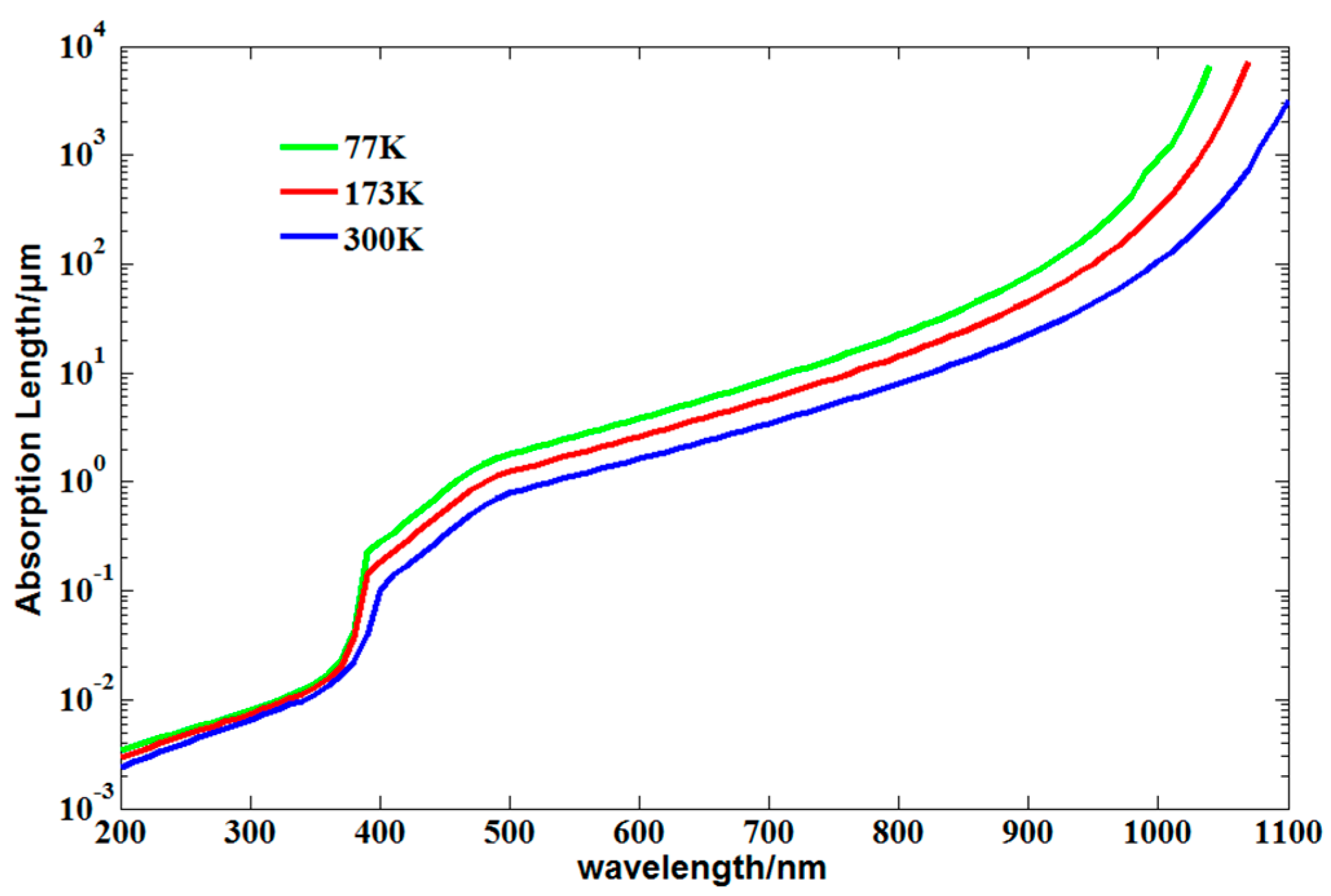
Back-illuminated CCDs are frequently used for astronomical applications due to their superior performance in terms of quantum efficiency, good linearity, and high spatial resolution [1]. However, a property of back-illuminated CCDs that is often overlooked is their propensity to generate constructive and destructive interference fringes when illuminated with coherent photons in NIR (near infrared, at wavelength within ~700–1100 nm) bands [2]. The absorption length, i.e., the path length required for 1/e (e is the natural constant) of the incoming photons to be absorbed in silicon, varies from about 0.1 μm (at 400 nm) to more than 100 μm (at 1000 nm), as shown in Figure 1. The typical thickness of the depletion region in back-illuminated thinned CCDs is about 10–50 μm [3]. The absorption length of NIR photons in silicon can be several times or even ten times this thickness, which indicates that the depletion region is semi-transparent in NIR. Consequently, the NIR photons will be reflected back and forth within the region. On the one hand, this can improve the quantum efficiency in NIR bands; on the other hand, interference fringes occur due to the multi-beam interference.
When back-illuminated CCDs are used in hyperspectral VNIR imagers, each pixel receives only extremely narrowband light, and the effects of interference fringes will appear when the spectral resolution is high enough (several nanometers or even less). Interference fringes appear from the wavelength of about 700 nm and can cause a sensitivity modulation as high as 40% [4], which greatly affects the spectral signals and image quality in NIR bands. Interference fringes vary rapidly as a function of wavelength, which is referred to as spectral fringing. Spatial fringing consists of two parts: (1) since the surfaces of the depletion region are not perfectly parallel or flat, local variations of the depletion region thickness can change the interference conditions, alter spectral fringing pattern, and result in spatial fringing; (2) due to the small-scale roughness of the imager’s entrance slit, there is fixed-pattern non-uniformity between pixels in the spatial dimension. Therefore, the fringing pattern is a combination of both spectral and spatial contributions and is irregular in both dimensions. In addition, since the refractive index and extinction coefficient of silicon are temperature-dependent [5] and cooling will induce small mechanical changes in the active silicon structure, the fringing pattern will change with the operating temperature of CCD, creating quite a complicated problem.
Interference fringing is an annoyance for many astronomical hyperspectral VNIR imagers. As for the removal of interference fringes, there are two types of methods. One is derived from improving the CCD device itself, such as increasing the thickness of depletion region [6], designing graded AR (Anti-Reflection) coatings to match the wavelength for each column of pixels [7,8], or conducting ‘roughening’ process of the back surface [4]. However, increasing the thickness of the depletion region will sacrifice the quantum efficiency in the blue, while designing graded AR coatings is quite complex and may increase the costs; conducting a ‘roughening’ process of the back surface does not show significant improvement in suppressing fringes.
The other method is from the perspective of post-processing. A model function to predict the fringing from STIS (the Space Telescope Imaging Spectrograph) G750L in HST (the Hubble Space Telescope) was proposed and used to defringe the object data [9]. However, the modeling requires a detailed knowledge of the CCD’s physical structure, which is difficult to scale. Moreover, the model is quite specific to the instrument and it is difficult to apply it to a situation where there is a wavelength shift problem. The flat-field method is a commonly used method. It is effective for data calibration when the fringe pattern does not change with time [10]. However, for the object data, previously observed flat fields could lead to a poor defringing result due to the wavelength shift problem [11,12]. Therefore, contemporaneous tungsten flat fields are suggested to correct fringes for STIS NIR long-slit spectra. On the one hand, this will take up valuable imaging time. On the other hand, flat fields and object data do not always share the same fringe pattern because variations in the illumination spectral characteristics can change the pattern’s amplitude or period. Therefore, flat fields could add a second set of fringes to the object data.
A method to remove fringes from images using wavelets was proposed by Rojo and Harrington [13]. It is an effective method to remove fringes from flat-field images, but its application to object images is not that useful since the fringe pattern is seldom regular with variations in the amplitude, frequency, and phase. A two-dimensional PCA (principal component analysis) was proposed to identify and isolate fringe structures from spectro-polarimetric data [14]. However, determining the number of PCA eigenvalues for the reconstruction of spectro-polarimetric data in order to attain the best compromise between fringe removal and original spectral signal preservation is quite difficult. Moreover, many of the PCA eigenvalues that contribute to the fringe pattern will also contain information of the spectral signals. Thus, this method is hardly automatic and may not be that effective.
From the above, the existing fringe removing methods are not quite suitable for dispersive hyperspectral VNIR imagers using back-illuminated CCDs. In this study, a two-step method to remove fringes is proposed, which can be performed automatically and is not specific to any instrument. The proposed method was applied to both calibration data and ground data in order to evaluate the performance.
The manuscript is organized as follows. We illustrate the details of our method in Section 2. In Section 3, we demonstrate the calibration data and ground data collected from two VNIR grating-based hyperspectral imagers using back-illuminated CCDs. In Section 4, we give a full evaluation of our method from the perspective of both image quality and spectral fidelity. Finally, we give the corresponding conclusions in Section 5.
2. Methods
For dispersive hyperspectral VNIR imagers using back-illuminated CCDs, the two dimensions of the CCD are used for spectral and spatial dimensions. They include a long and narrow slit that controls a strip of area being imaged along the cross-track direction. A dispersive hyperspectral VNIR imager captures a single cross-track line at one time for all bands, while the other spatial dimension along the flight direction is obtained through push-broom scanning. Here, the cross-track pixels and wavelength channels are represented as samples and bands, respectively. The number of samples is denoted as N, and the number of bands is denoted as M. We indicate with , for , a set of images (e.g., the sequential series of the frames collected in the along-track direction), each represented by a matrix. For each frame obtained, the expected response value is modulated by fringes, and it can be expressed as:
where is the fringing amplitude, is the expected response value, and is the observed response value. The goal of correction is to determine the coefficients for each pixel in each frame such that:
where is the correction coefficient and is the recovered response value.
A two-step correction method is proposed to determine the correction coefficients for each pixel at each frame.
(1) Step 1: spectral fringing suppression
For each frame, the neighboring bands see the same objects in very close wavelength, and they should have similar response values for the same sample. However, due to the modulation effect of interference fringes, the spectral response curve shows high frequency spikes. The expected spectral response curve should be smooth, which can be achieved by using a ridge regression model. The potential risk of ridge regression is that it may reduce the contrast of fine spectral signatures. In order to attain the best compromise between fringe removal and the preservation of original spectral signatures, a ridge regression model based on a moving window is adopted for spectral fringing suppression.
The original spectral response curve is denoted as . Suppose the spectral fringing starts from band P (1 < P < M), and the moving window size is , then the spectral response curve within the sliding window is given by:
where is the center band of the sliding window, and “” represents that it takes continuous values from to in . When is greater than M, a symmetrical extension is adopted to handle the boundary problem.
where .
The ridge regression result of is denoted as , and we have,
where is obtained from the ridge regression model, and is given by:
where is the model parameters of the ridge regression model.
The objective function of ridge regression model is given by [15]:
where is the model parameters to be solved, and is a regularization parameter. is generated from a Gaussian kernel function, and is defined as:
where is the value of the position in the matrix .
By setting , we have:
For band , the above process is repeated. Since the preceding P bands are not affected by interference fringes, keeps the original value unchanged for these bands. For each column in , the ridge regression is repeated, and the correction result is denoted as .
The selection of is an art. A too large makes the model parameters tend to zero, whereas a too small makes the effect of regression degrade. So a balance point exists between zero and infinity, where the ridge regression model achieves the best performance. One way to determine is to take use of the calibration data acquired in laboratory conditions, i.e., the optimal is obtained by minimizing the spectral fringes of the calibration data.
(2) Step 2: spatial fringing suppression
After suppressing spectral fringes in step 1, in step 2, a SSR (Spectral-Spatial Ratio) method adapted from [16] is adopted for the removal of spatial fringes.
First, the sequential series of frames () from Step 1 are reorganized as (a matrix) by bands, for . The column (a vector) in is a transpose of row (a vector) from . Here, we denote , as the row , of , and , as the row , of . For hyperspectral data, there is a strong relationship between neighboring spectral ratios, i.e., for each combination of band pairs, we have assumptions expressed as follows:
where “” is point-multiplication, takes the median value of the expression, and is the correction coefficient for band , sample .
First, is initialized to 1 for , then , , is solved sequentially from Equation (10) using the least squares method. However, statistically noisy values for ratios will cause the magnitude of to slowly “drift” as we move further from to . In order to eliminate the effects of “drift”, drift trend has to be estimated reasonably.
For each band, , is separated into groups with each 16 consecutive coefficients per group. Then, the median value of each group is calculated, and the result is denoted as (a vector), from which a Fourier interpolation method is used to estimate the drift trend.
First, discrete Fourier transformation is performed to ,
Then, the n () low frequency components are used for Fourier interpolation. To do this, a vector is defined as:
Finally, inverse discrete Fourier transformation is performed to ,
where is the final estimated drift trend.
For each band, , , is normalized by ,
Then the correction of is performed,
where , , and is the correction result. For , Equations (10)–(15) is repeated.
In fact, there is another strategy to solve the correction coefficient . After solving Equations (10)–(15) for a combination of band pairs, the two corrected bands can be used as references to correct the neighboring bands. Assume that for band b have been solved, then for band b + 1 can be solved sequentially from to with initialized to 1. The iteration equation is given by:
For each band, the average of over samples is supposed to close to 1. Then, , , is normalized by ,
where is given by
One of the advantages of this strategy is that it does not need to estimate the drift trend for the rest bands. We have made three assumptions in Equation (10), of which the first is a much more statistical stable relationship while the other two would cause the drift problem. This strategy uses only the first assumption and can avoid the drift problem.
3. Materials
To evaluate the performance of the proposed method, two typical VNIR grating-based hyperspectral imager designed by SITP (Shanghai Institute of Technical Physics) are used. They are both push-broom hyperspectral imagers using thinned, back-illuminated CCDs. Camera 1 measures in the 400~1000 nm spectral range with a spectral sampling of 4.3 nm, and Camera 2 measures in the 400~1050 nm spectral range with a spectral sampling of 2.15 nm. The calibration data was collected in laboratory conditions where a uniform, diffuse light source (Tungsten Lamp) from an integrating sphere was taken as the flat-field source; and the ground data was collected outdoors through a two-dimensional rotating platform that helps to achieve push-broom scanning.
(1) Calibration Data
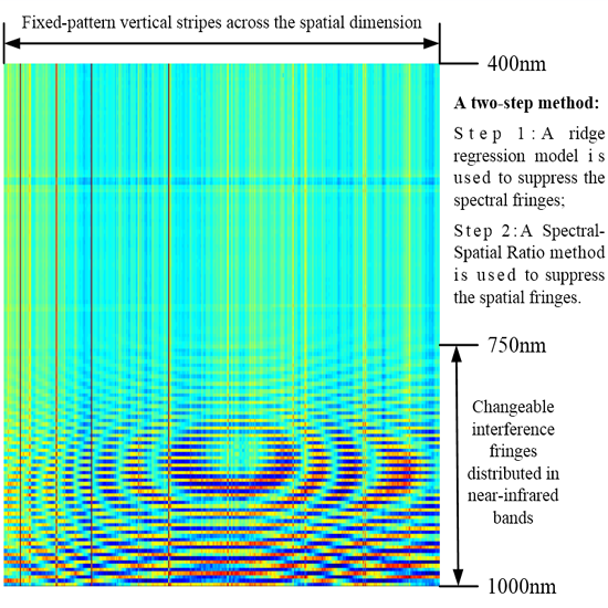
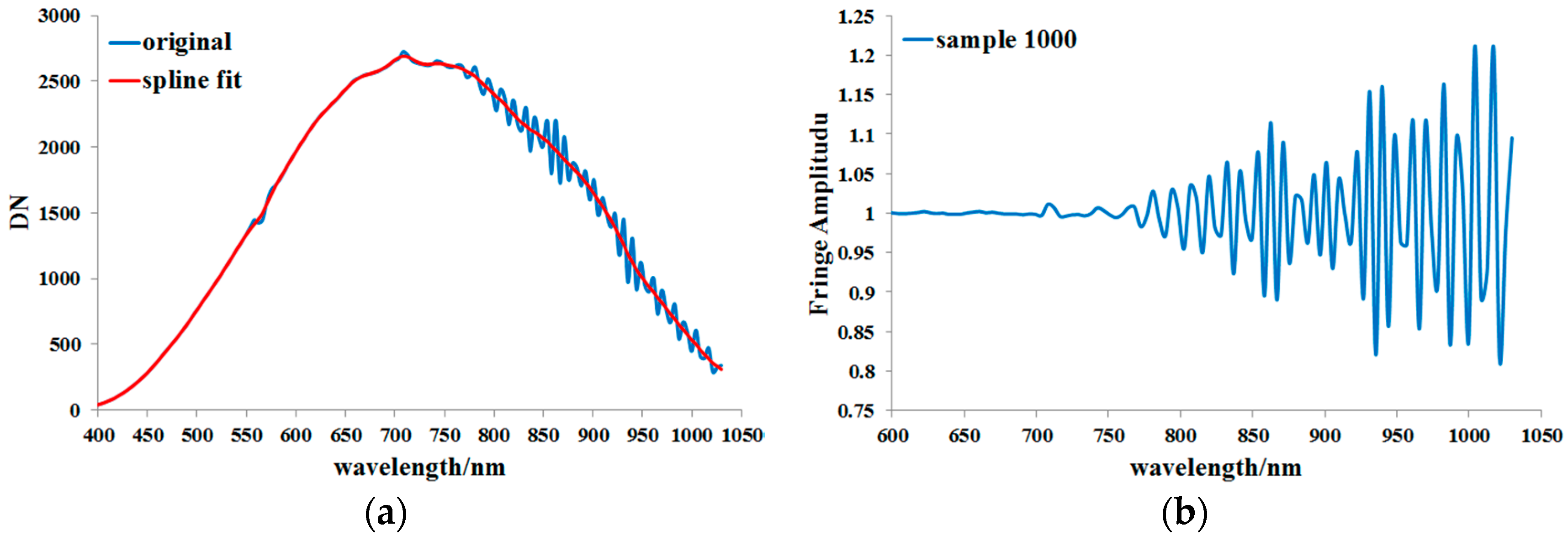
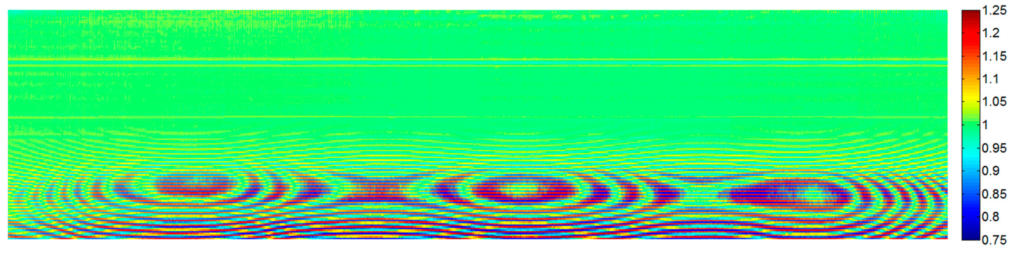
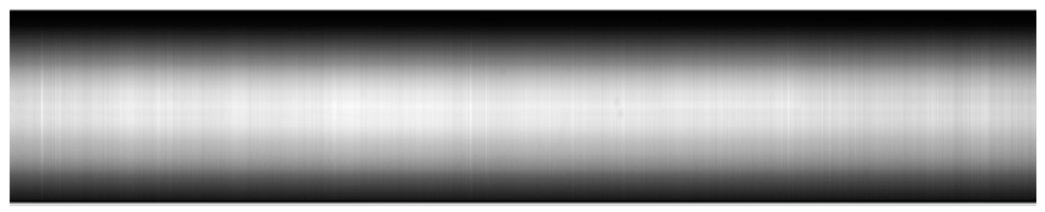
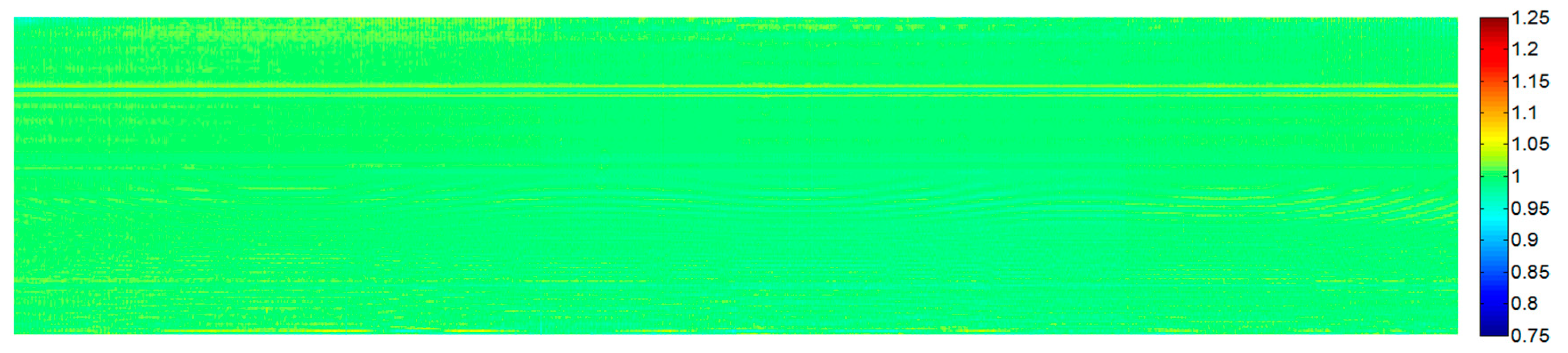
The acquired calibration data (150 bands by 2048 samples) from Camera 1 is shown in Figure 2. There are obvious interference fringes in the NIR bands. In addition to the interference fringes, there are vertical stripes (fixed-pattern non-uniformity) distributed along the spatial dimension. The fringe-free data is obtained through a spline fit of the calibration data in spectral dimension; then, the fringe amplitude of each pixel is obtained when the fringe data is divided by the fringe-free data. The DN (Digital Number) response curve along sample 1000 and its spline fit result are shown in Figure 3a. The fringe amplitude along sample 1000 is presented in Figure 3b, where the spectral fringes become serious for wavelength longer than 760 nm. Figure 4 shows the fringe amplitude image of the calibration data. The interference pattern is a combination of both spectral and spatial contributions, and does not show any obvious regularity.
(2) Ground Data
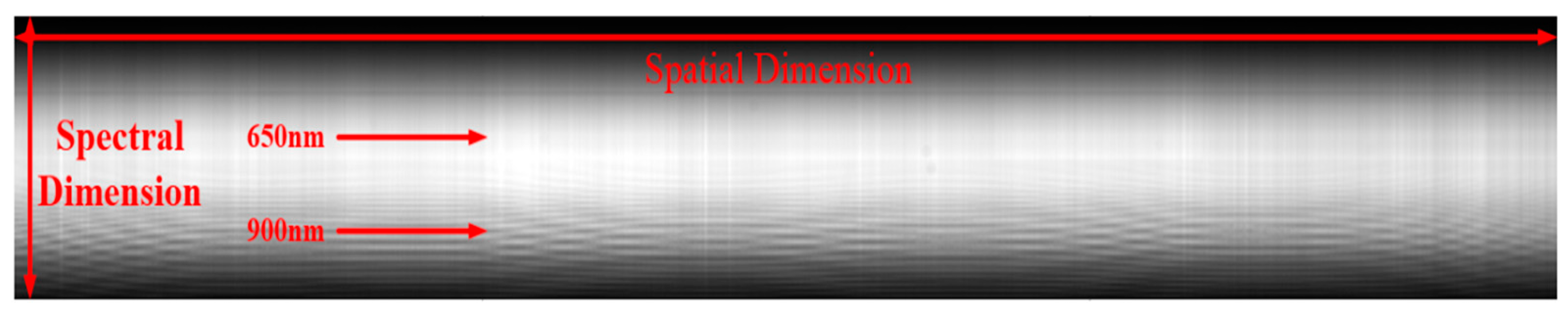
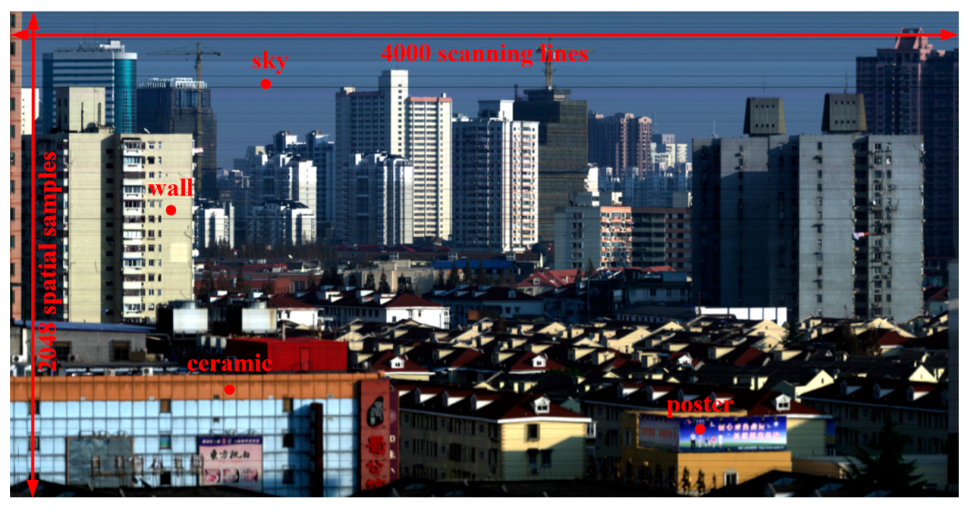
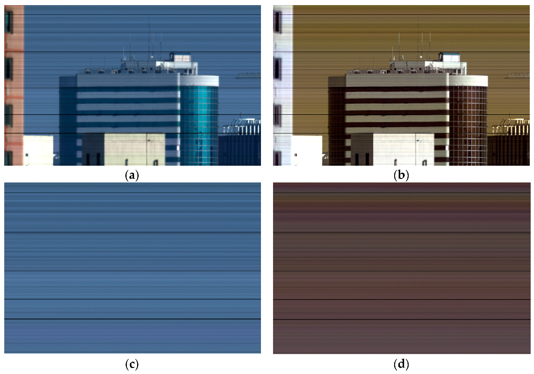
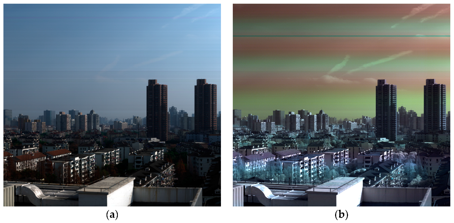
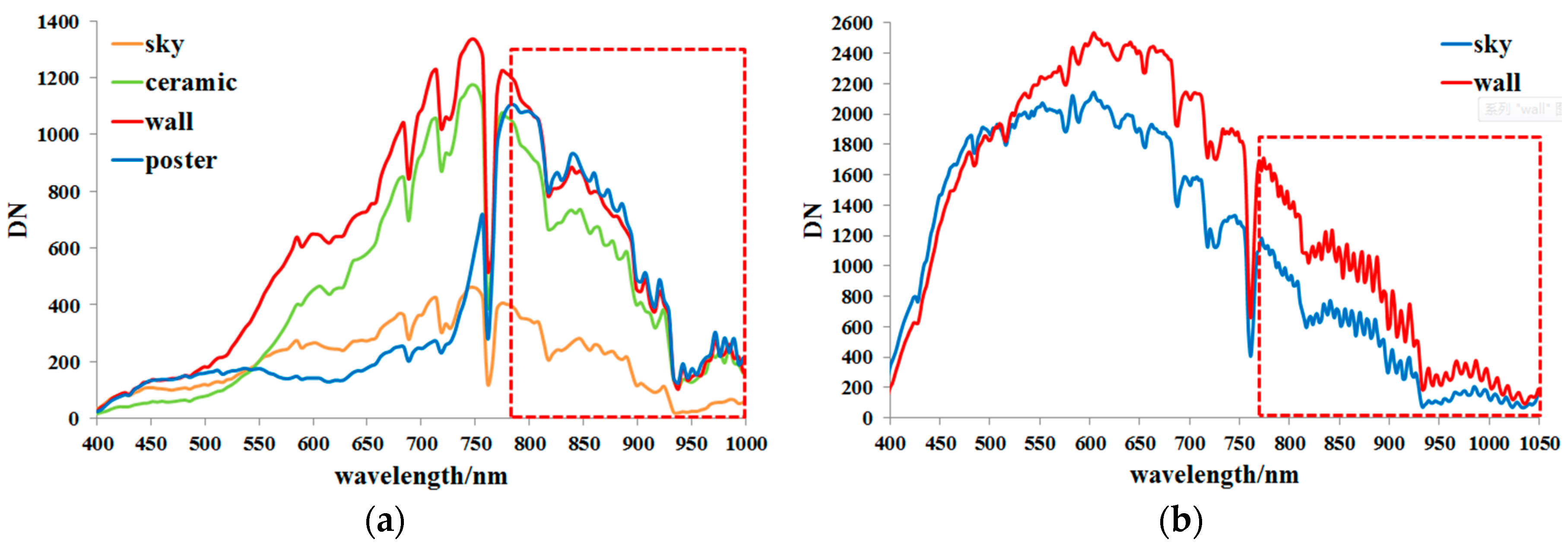
The collected ground data from Camera 1 is shown in Figure 5. It consists of 4000 scanning lines with 2048 spatial samples per frame in the cross track direction. Two sub-images in visible bands are shown in Figure 6a,c, and two sub-images of the same region in NIR bands are shown in Figure 6b,d. In Figure 6a,c, the horizontal stripes are caused by the fixed-pattern non-uniformity. While in Figure 6b,d, in addition to the stripes caused by fixed-pattern non-uniformity, there are rainbow-like stripes, which are the results of interference, and they become obvious in Figure 6d. The collected ground data from Camera 2 is shown in Figure 7. It consists of 2200 scanning lines with 2048 spatial samples per frame in the cross track direction. In Figure 7a, no interference fringes are presented, while they are quite obvious in Figure 7b. Compared with Camera 1, Camera 2 suffers much more serious interference fringes in NIR bands due to its higher spectral resolution. A good thing for Camera 2 is that it suffers little from the fixed-pattern non-uniformity problem. The spectral response curves of the four typical targets marked in Figure 5 are shown in Figure 8a, and the spectral response curves of two typical targets acquired by Camera 2 are shown in Figure 8b. As illustrated in the red box, all the spectra suffer from serious spectral fringes for wavelength longer than 760 nm, especially for those acquired by Camera 2, since a higher spectral resolution will result in more serious interference.
4. Results and Discussion
For both the calibration data and the ground data collected from Camera 1, during the correction process in Step 1, the widow size L (Equation (3)) takes the value of 4, regularization parameter takes the value of 0.12, and (Equation (8)) in Gaussian kernel function takes the value of 1.5. For the ground data collected from Camera 2, L takes the value of 4, takes the value of 0.3, and takes the value of 3.5. The empirical parameters (L, , and ) are determined by minimizing the spectral fringes of the calibration data acquired in laboratory conditions.
(1) Calibration Data
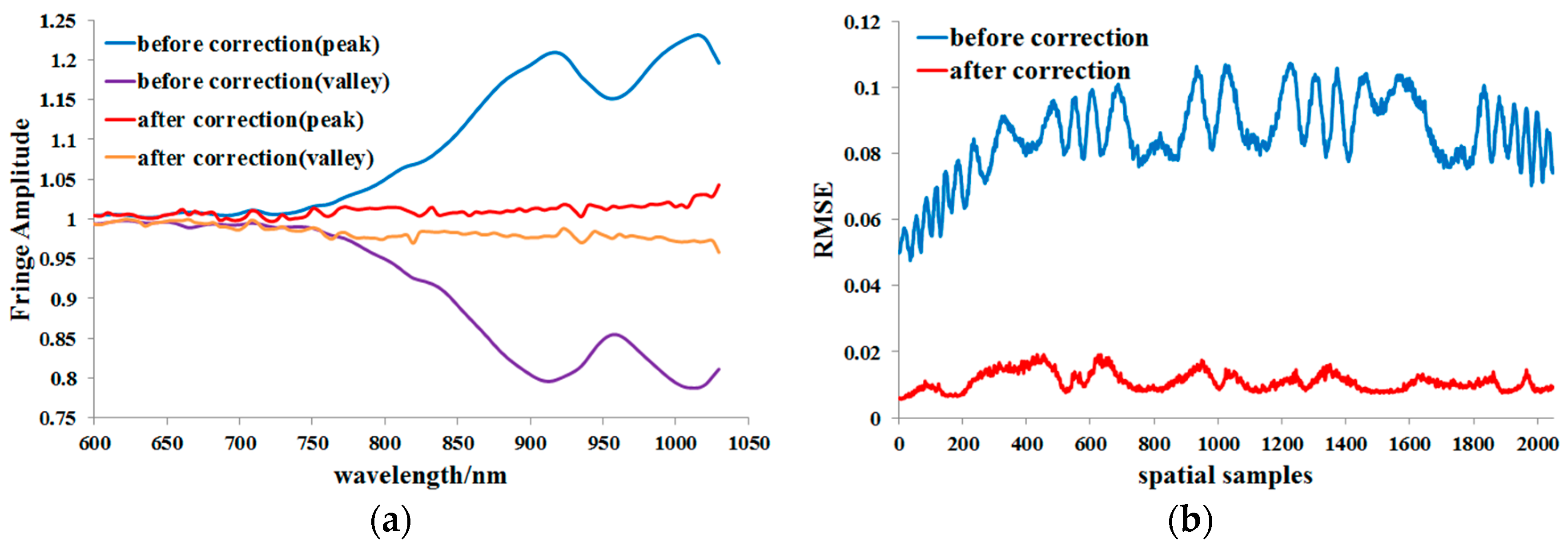
Since the data acquired in the laboratory did not involve the push-broom scanning process, only Step 1 can be done to the calibration data. Figure 9 shows the correction result of calibration data after Step 1, and Figure 10 shows the fringe amplitude image after correction. As the two figures show, the interference fringes have been greatly suppressed. The spatial fringing caused by interference is interdependent with the spectral fringing. Therefore, when the spectral fringing is effectively suppressed, the spatial fringing is suppressed at the same time, and the remaining spatial fringes are mainly the fixed-pattern non-uniformity. The peak and valley fringe amplitudes of each band are presented in Figure 11a. Before correction, the fringe amplitudes can be as high as ±23%; after correction, the fringe amplitudes are within ±4%. For each column of the fringe amplitude image, the RMSE (Root Mean Square Error) is calculated, and the results are shown in Figure 11b. Before correction, the RMSE was as high as 10.7%; after correction, the RMSE is less than 1.9%. The proposed method can suppress the interference fringes by a factor of more than 5.6.
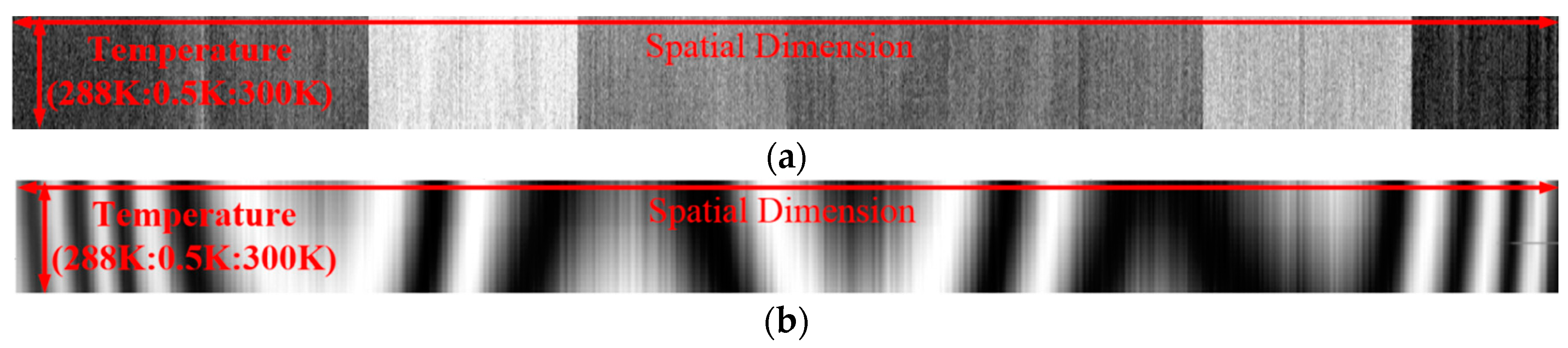
Another way to correct the fringes is using the flat-field data collected in laboratory conditions, where a uniform, diffuse light source from an integrating sphere was taken as the flat-field source. Figure 12 shows the correction result of calibration data using flat-field method. Though the vertical stripes have been removed, the interference fringes remain uncorrected. This is because the fixed-pattern non-uniformity across the spatial dimension can be calibrated from the flat-field data. However, the interference fringes cannot be calibrated since they are changing with the CCD operating temperature, as shown in Figure 13. Since band 75 () is free from interference, no noticeable effect from the CCD operating temperature is presented. However, the fringe pattern of band 120 () is changing rapidly with the increasing of CCD operating temperature. Therefore, the flat-field data and the calibration data are very likely to share different fringe patterns due to the changes in CCD operating temperature.
(2) Ground Data
For the ground data, Step 1 is performed from band 86 (). Then, the spatial correction coefficients are solved for each band, which will suffer from the increasing “drift” problem as we move further from the original sample. To estimate the drift trend, a Fourier interpolation method is used, of which the difficult part is to determine the number of low frequency components used for Fourier interpolation. In our case, there are 2048 spatial correction coefficients (N = 2048) for each band, and they are divided into 128 groups with each 16 consecutive coefficients per group. After discrete Fourier transformation is performed to the vector consisted of the median values of the 128 groups, there will be 128 frequency components, and 10 low frequency components (n = 10) are used for Fourier interpolation. Finally, the normalized spatial correction coefficients can be obtained by eliminating the drift trend from the estimated spatial correction coefficients. Figure 14a shows the estimated coefficients of band 60 and the corresponding drift trend, and Figure 14b shows the normalized spatial correction coefficients. As the two figures show, the estimation of the drift trend is reasonable.
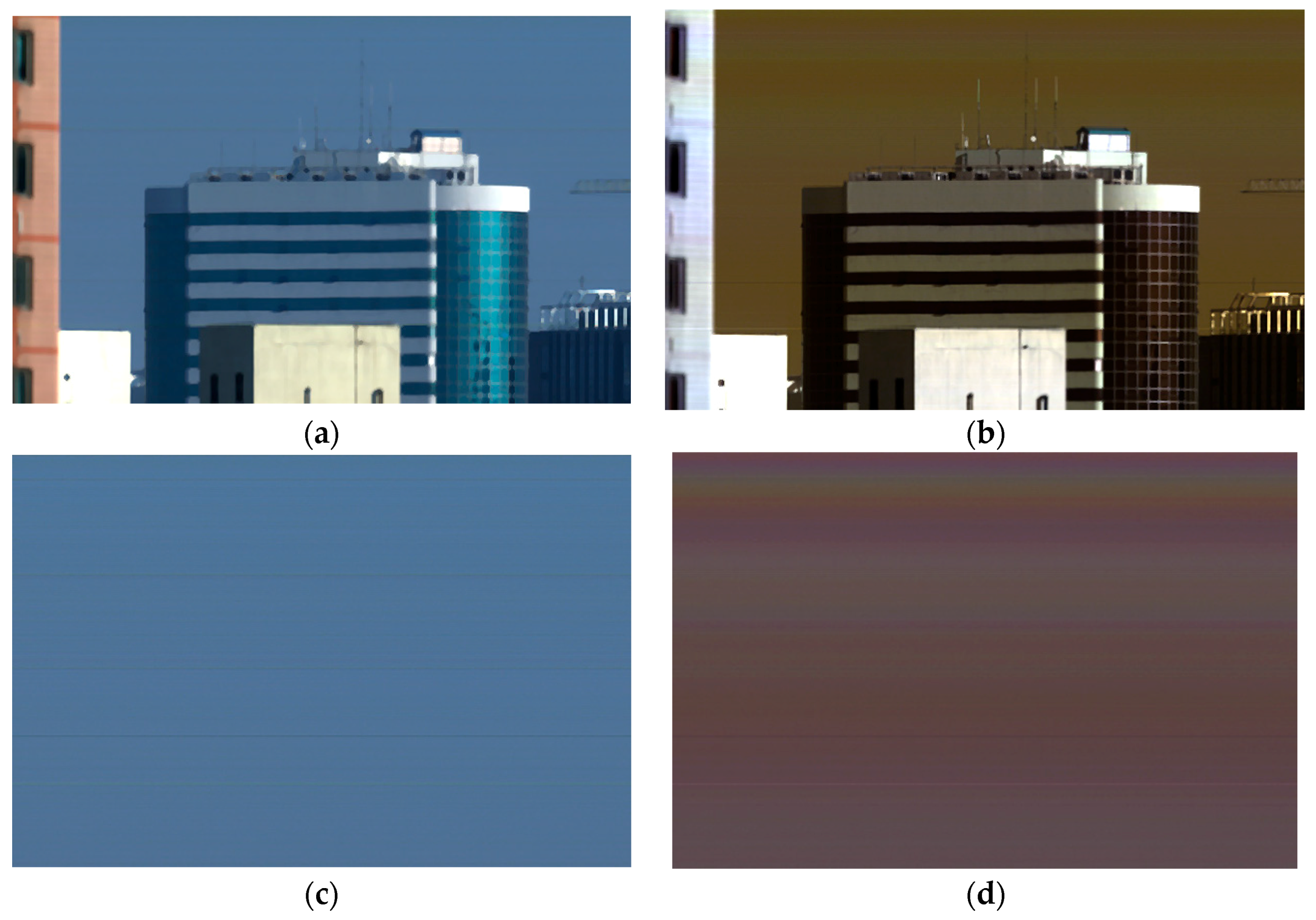
After the ground data from Camera 1 was corrected using the proposed method, four sub-images are shown in Figure 15. The spatial fringes caused by fixed-pattern non-uniformity have been removed. For the two sub-images in NIR bands, though no obvious interference fringes are shown in Figure 15b, there are still some subtle interference fringes remaining in Figure 15d, indicating that the proposed method still needs further improvement. As a comparison, the correction results of the ground data using the flat-field method are presented in Figure 16. For the two sub-images in visible bands, the stripes have been largely suppressed, and the remaining subtle stripes are due to the fact that there will also be a slight change of non-uniformity with time. For the two sub-images in NIR bands, though the fixed-pattern stripes have been well suppressed, the interference fringes remain, and they are quite serious in Figure 16d, indicating the inability of the flat-field method in correcting the interference fringes. Therefore, both methods perform quite well on the correction of fixed-pattern non-uniformity, while only the proposed method is effective for suppressing the interference fringes. From the perspective of image quality, the proposed method offers a much more satisfactory result.
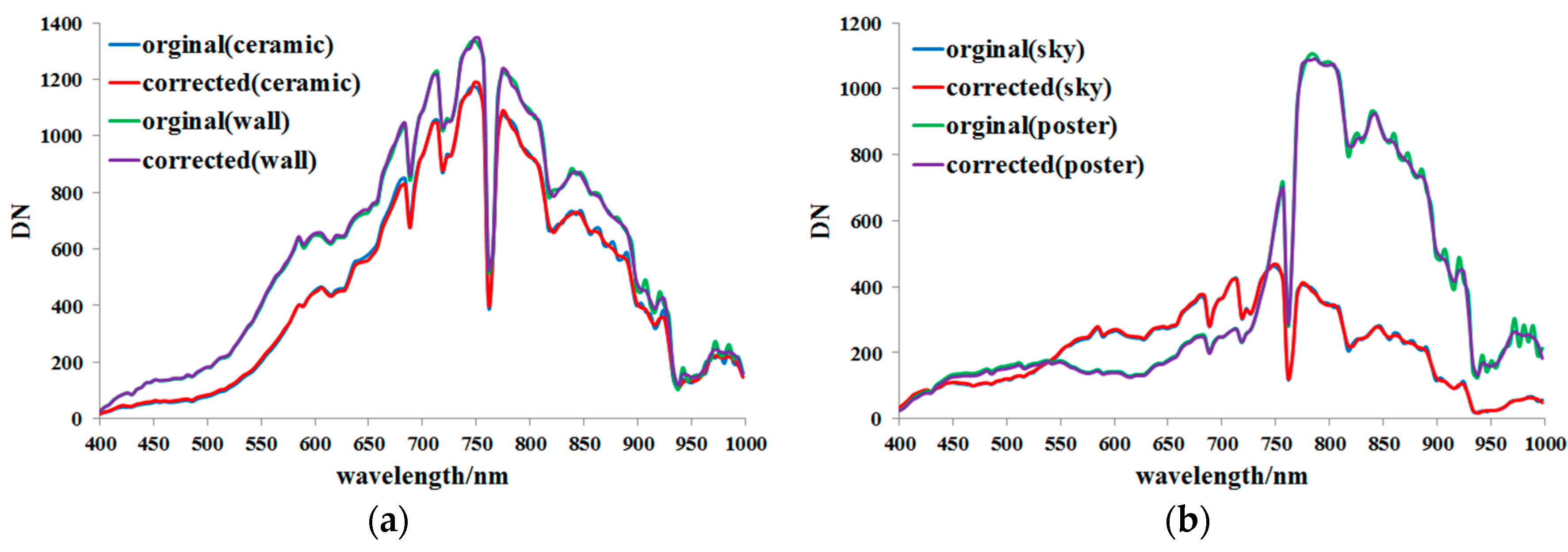
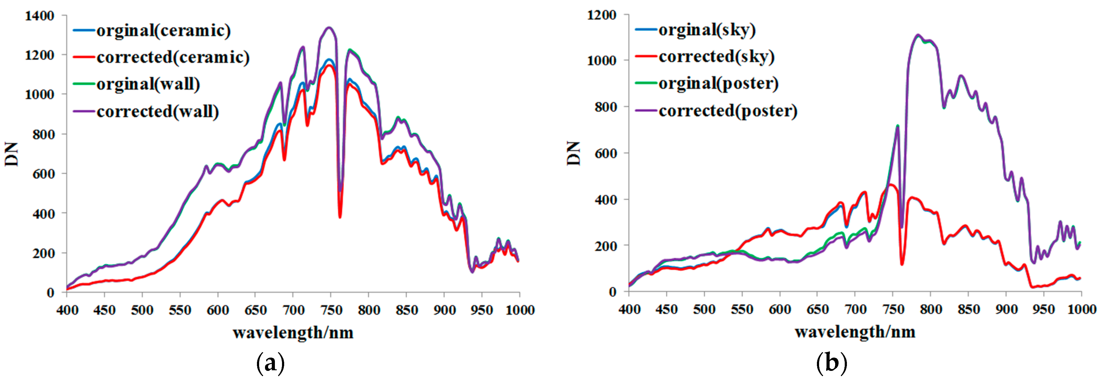
After the ground data is corrected using the proposed method, the reconstructed spectral response curves of the four typical targets are shown in Figure 17. Before correction, there are obvious spectral fringes in NIR band; after correction, spectral fringes have been largely suppressed, and the spectral shape before and after correction shows reasonable consistency. After the ground data are corrected using the flat-field method, the reconstructed spectral response curves of the four typical targets are nearly the same before and after correction, as shown in Figure 18. There are two major factors that cause the flat-field method not able to correct the spectral fringes, one is the changing of CCD operating temperature, and the other is the illumination spectral signatures, which will also alter the interference conditions and result in a much more complicated fringe patterns. Since the spectral curves of ground objects cannot be known in advance, quantitative evaluations of the correction accuracy cannot be carried out.
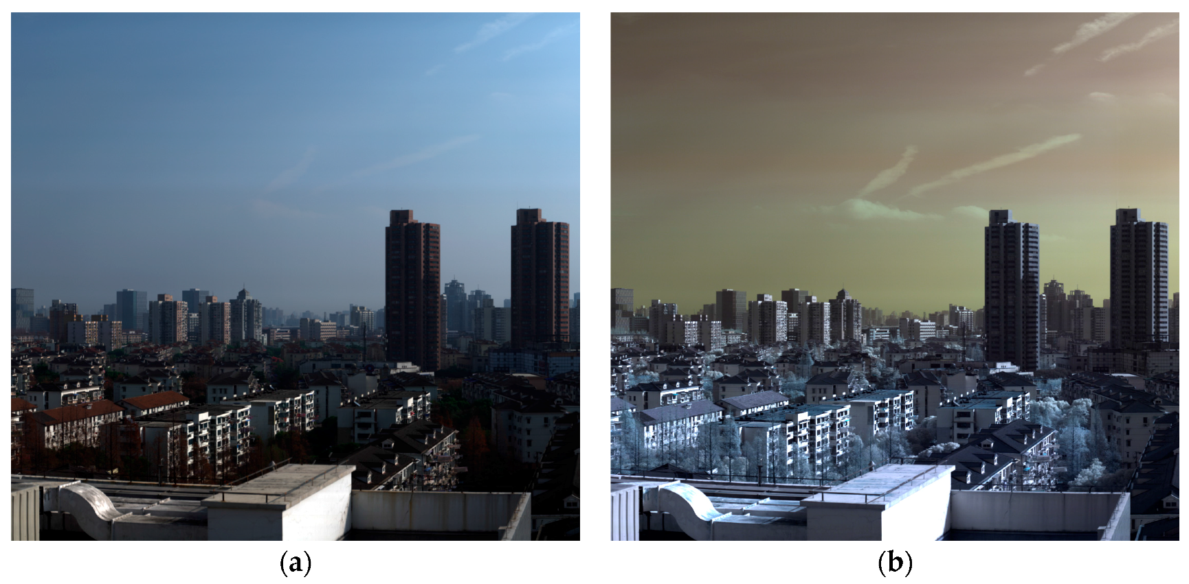
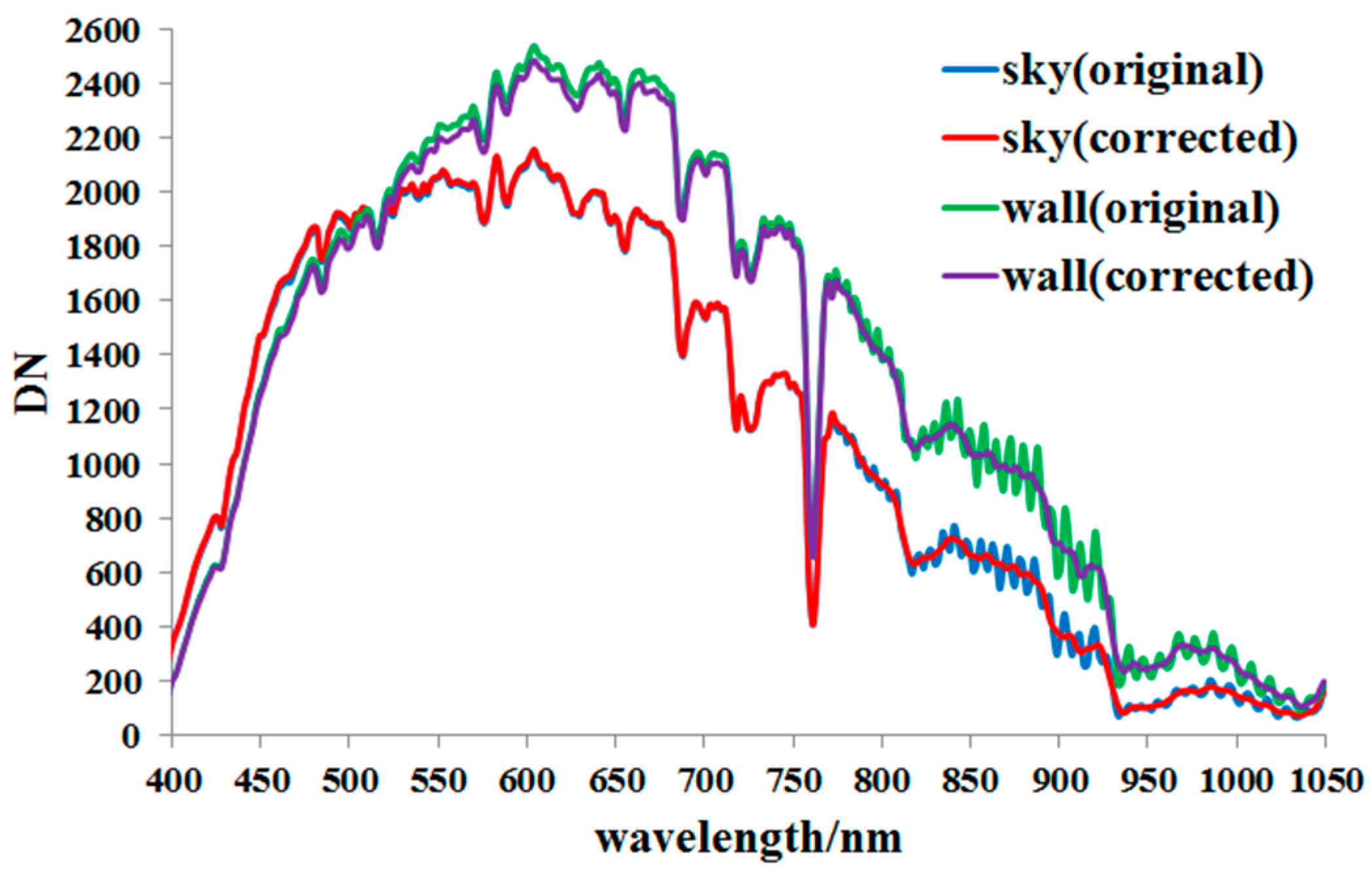
Again, the proposed method was used to correct the ground data from Camera 2, and the results are shown in Figure 19a,b, respectively. The spatial fringes in both the visible bands and NIR bands have been properly corrected. In particular, the interference fringes in Figure 19b are hardly noticeable after correction. Besides, the spectral fringes at the wavelength longer than 760 nm have been greatly suppressed, as shown in Figure 20, indicating the adaptability of our method.
5. Conclusions
We have presented a two-step method that allows us to remove fringes for hyperspectral VNIR imagers. This method is highly automated and provides satisfactory results in terms of image quality and spectral fidelity; it makes no assumptions about the instruments and thus should be transferable to other hyperspectral VNIR imagers.
The most difficult part for the removal of fringes is that the pattern of fringes is not fixed. It is sensitive to wavelength shift, operating temperature of CCD, and related to the illumination spectral characteristics. The proposed method shows flexible adaptability to these factors, which does not rely on any calibration data and computes correction coefficients from the object data itself. We have demonstrated that this method can reduce the peak fringe amplitude from about ±23% (10.7% RMSE) to about ±4% (1.9% RMSE). When applying this method to hyperspectral VNIR data with fringes, a sufficient number of scanning frames (usually hundreds to thousands) is necessary to guarantee the assumptions made between neighboring spectral–spatial ratios. Since there are hundreds of spectral bands for hyperspectral VNIR data, an improvement could be made if a much stronger relationship between band combinations can be found in solving correction coefficients.
Acknowledgments
This work was financially supported by the National Key R&D Program of China (2016YFB0500400), the National High Technology Research and Development Program of China (863 Program; 2014AA123202), Major Project of National High-Resolution Earth Observation System of China (A0106/1112).
Author Contributions
Binlin Hu established the two-step correction method and wrote the paper; Dexin Sun helped implement the correction procedures and analyzed the data; Binlin Hu and Yinnian Liu conceived and designed the experiments.
Conflicts of Interest
The authors declare no conflict of interest.
References
- Naletto, G.; Pace, E.; Tondello, G.; Boscolo, A. Performance of a thinned BI CCD as detector for normal incidence EUV spectrograph. Meas. Sci. Technol. 1994, 5, 1491–1500. [Google Scholar] [CrossRef]
- Groom, D.E.; Holland, S.E.; Levi, M.E.; Palaio, N.P.; Perlmutter, S. Back-illuminated, Fully-Depleted CCD image Sensors for use in Optical and near-IR Astronomy. Nucl. Instrum. Methods Phys. Res. 2000, 442, 216–222. [Google Scholar] [CrossRef]
- Bebek, C.J.; Coles, R.A.; Denes, P.; Dion, F.; Emes, J.H.; Frost, R.; Groom, D.E.; Groulx, R.; Haque, S.; Holland, S.E.; et al. CCD Research and Development at Lawrence Berkeley National Laboratory. In Proceedings of the SPIE Astronomical Telescopes + Instrumentation, Amsterdam, The Netherlands, 1–6 July 2012. [Google Scholar]
- Optical Etaloning in Charge Coupled Devices. Available online: http://www.andor.com/learning-academy/optical-etaloning-in-charge-coupled-devices-technical-article (accessed on 27 November 2017).
- Jellison, G.E.; Modine, F.A. Optical functions of silicon at elevated temperatures. J. Appl. Phys. 1994, 76, 3758–3761. [Google Scholar] [CrossRef]
- Groom, D.E. Recent progress on CCDs for astronomical imaging. Proc. SPIE 2000, 4008, 634–645. [Google Scholar]
- Andersen, M.I. Optimising CCDs for Spectrographs. Optical Detectors for Astronomy II; Amico, P., Beletic, J.W., Eds.; ASSL Series; Kluwer Academic Publishers: Dordrecht, The Netherlands, 2000; Volume 252, pp. 279–282. [Google Scholar]
- Kelt, A.; Harris, A.; Jorden, P.; Tulloch, S. Optimised CCD Antireflection Coating: Gradded Thickness AR Coating (for Fixed-Format Spectroscopy). Sci. Detect. Astron. 2005, 369–374. [Google Scholar] [CrossRef]
- Malumuth, E.M.; Hill, R.S.; Gull, T.; Woodgate, B.E.; Bowers, C.W.; Kimble, R.A.; Lindler, D.; Plait, P.; Blouke, M. Removing the Fringes from Space Telescope Imaging Spectrograph Slitless Spectra. Publ. Astron. Soc. Pac. 2003, 115, 218–234. [Google Scholar] [CrossRef]
- Ma, L.; Wei, J.; Huang, X.X. Research on and Correction of Interference Fringes Phenomenon in Dispersive Hyperspectral Imaging Spectrometer Using BI CCDs in Near-Infrared Band. Spectrosc. Spectr. Anal. 2014, 34, 1995–1999. [Google Scholar]
- Walsh, J.R.; Baum, S.A.; Malumuth, E.M.; Goudfrooij, P. STIS Near-IR Fringing: Basics and Use of Contemporaneous Flats for Extended Sources. STIS Instrument Science Report 97-16. 1997. Available online: https://www.researchgate.net/publication/251303703_STIS_Near-IR_Fringing_Basics_and_Use_of_Contemporaneous_Flats_for_Extended_Sources (accessed on 8 January 2018).
- Howell, S.B. Fringe Science: Defringing CCD Images with Neon Lamp Flat Fields. Publ. Astron. Soc. Pac. 2012, 124, 263–267. [Google Scholar] [CrossRef]
- Rojo, P.M.; Harrington, J. A Method to Remove Fringes from Images Using Wavelets. Astrophys. J. 2006, 649, 553–560. [Google Scholar] [CrossRef]
- Casini, R.; Judge, P.G.; Schad, T.A. Removal of Spectro-Polarimetric Fringes by Two-Dimensional Pattern Recognition. Astrophys. J. 2012, 756, 828–842. [Google Scholar] [CrossRef]
- Hoerl, A.E.; Kennard, R.W. Ridge Regression: Biased Estimation for Nonorthogonal Problems. Technometrics 2000, 42, 80–86. [Google Scholar] [CrossRef]
- Fischer, A.D.; Thomas, T.J.; Leathers, R.A.; Downes, T.V. Stable Scene-Based Non-Uniformity Correction Coefficients for Hyperspectral SWIR Sensors. In Proceedings of the IEEE Aerospace Conference, Big Sky, MT, USA, 3–10 March 2007; pp. 1–14. [Google Scholar]
Figure 1.
Absorption length in silicon versus wavelength at temperatures of 77, 173, and 300 K.

Figure 2.
The calibration data acquired from Camera 1.

Figure 3.
(a) DN response curves along sample 1000 and its spline fit result; (b) fringe amplitude along sample 1000.
Figure 3.
(a) DN response curves along sample 1000 and its spline fit result; (b) fringe amplitude along sample 1000.

Figure 4.
The fringe amplitude image of the calibration data.

Figure 5.
RGB image in visible bands from Camera 1 (R: 650 nm, G: 560 nm, B: 480 nm).

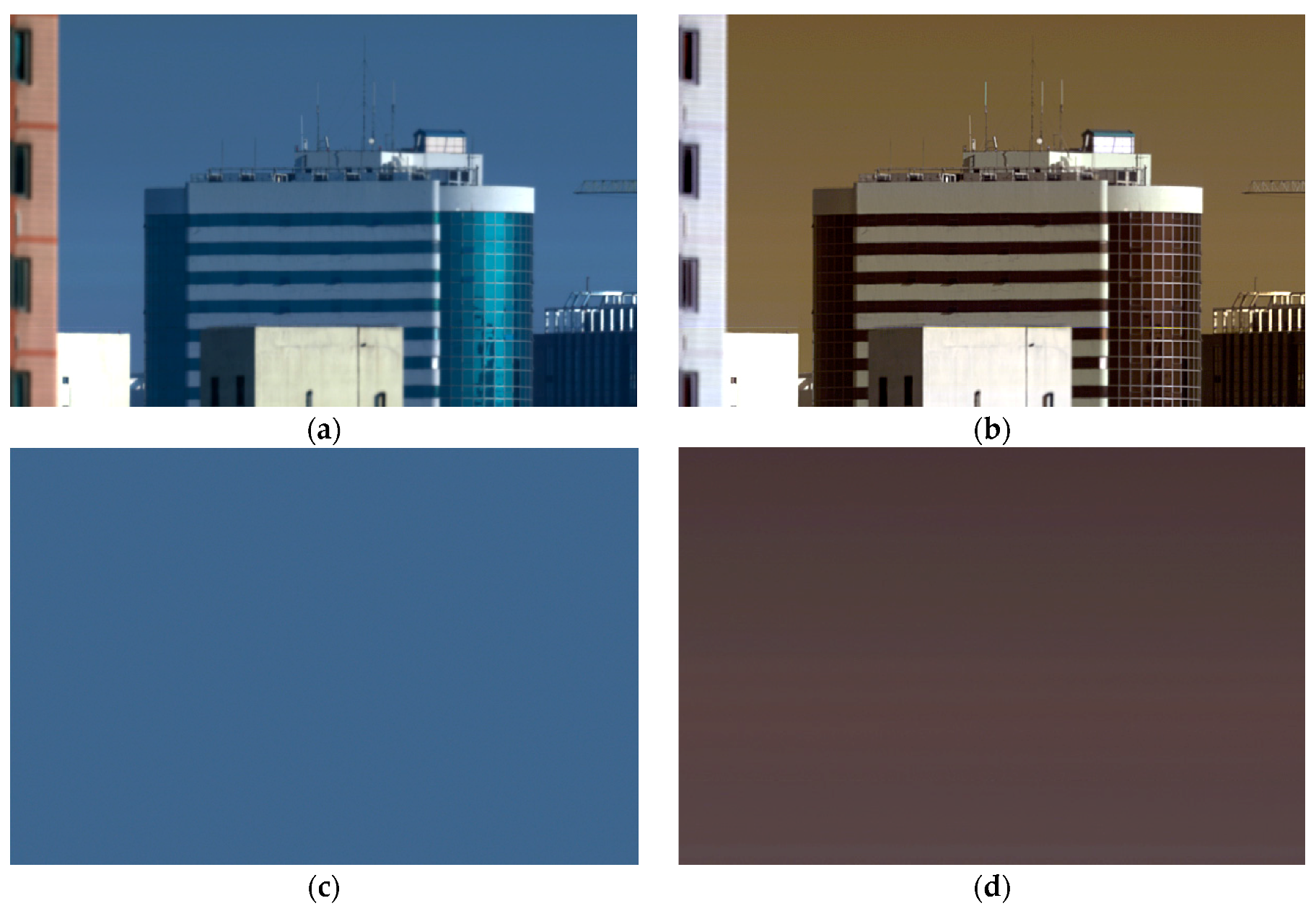
Figure 6.
(a) A sub-image of “buildings” in visible bands (R: 650 nm, G: 560 nm, B: 480 nm); (b) A sub-image of “buildings” in NIR bands (R: 740 nm, G: 825 nm, B: 955 nm); (c) A sub-image of “the sky” in visible bands (R: 650 nm, G: 560 nm, B: 480 nm); (d) A sub-image of “the sky” in NIR bands (R: 825 nm, G: 912 nm, B: 976 nm).

Figure 7.
Image data collected from Camera 2. (a) RGB image in visible bands (R: 650 nm, G: 560 nm, B: 480 nm); (b) False-color RGB image in NIR bands (R: 800 nm, G: 890 nm, B: 960 nm).
Figure 7.
Image data collected from Camera 2. (a) RGB image in visible bands (R: 650 nm, G: 560 nm, B: 480 nm); (b) False-color RGB image in NIR bands (R: 800 nm, G: 890 nm, B: 960 nm).

Figure 8.
(a) Spectral response curves of four typical targets acquired by Camera 1; (b) Spectral response curves of two typical targets acquired by Camera 2.
Figure 8.
(a) Spectral response curves of four typical targets acquired by Camera 1; (b) Spectral response curves of two typical targets acquired by Camera 2.

Figure 9.
The correction result of calibration data after Step 1.

Figure 10.
The fringe amplitude image after Step 1.

Figure 11.
(a) The peak and valley fringe amplitudes before and after correction; (b) RMSE is calculated for each column of the fringe amplitude image before and after correction.
Figure 11.
(a) The peak and valley fringe amplitudes before and after correction; (b) RMSE is calculated for each column of the fringe amplitude image before and after correction.

Figure 12.
The correction result of calibration data using flat-field method.

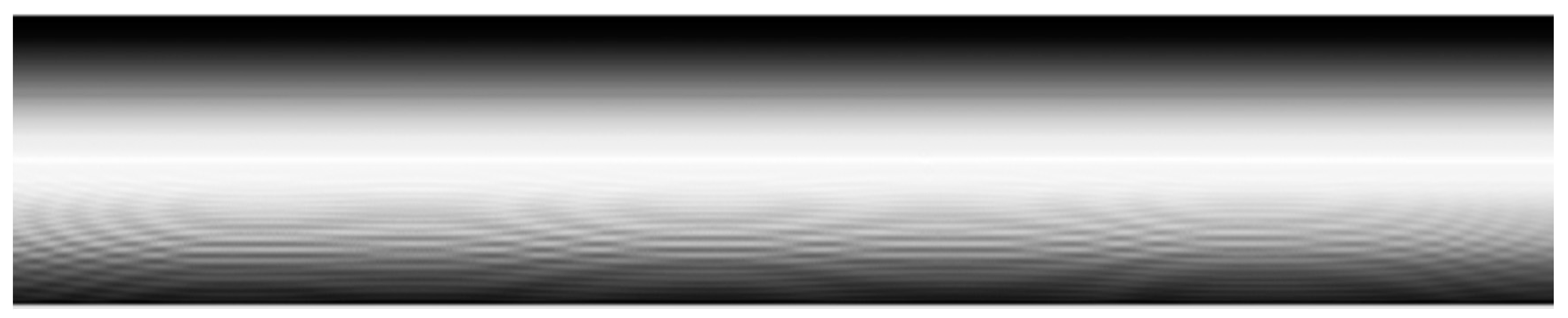
Figure 13.
A sequential series of flat-field frames (150 bands by 2048 columns) were collected with the increasing of the CCD operating temperature, then the sequential series of (a) band 75 and (b) band 120 from each frame are presented with the increasing of the CCD operating temperature.
Figure 13.
A sequential series of flat-field frames (150 bands by 2048 columns) were collected with the increasing of the CCD operating temperature, then the sequential series of (a) band 75 and (b) band 120 from each frame are presented with the increasing of the CCD operating temperature.

Figure 14.
(a) Estimated coefficients of band 60 and the corresponding drift trend; (b) Normalized coefficients.
Figure 14.
(a) Estimated coefficients of band 60 and the corresponding drift trend; (b) Normalized coefficients.

Figure 15.
Correction results of the ground data using the proposed method. (a) A sub-image of “buildings” in visible bands (R: 650 nm, G: 560 nm, B: 480 nm); (b) A sub-image of “buildings” in NIR bands (R: 740 nm, G: 825 nm, B: 955 nm); (c) A sub-image of “the sky” in visible bands (R: 650 nm, G: 560 nm, B: 480 nm); (d) A sub-image of “the sky” in NIR bands (R: 825 nm, G: 912 nm, B: 976 nm).

Figure 16.
Correction results of the ground data using the flat-field method. (a) A sub-image of “buildings” in visible bands (R: 650 nm, G: 560 nm, B: 480 nm); (b) A sub-image of “buildings” in NIR bands (R: 740 nm, G: 825 nm, B: 955 nm); (c) A sub-image of “the sky” in visible bands (R: 650 nm, G: 560 nm, B: 480 nm); (d) A sub-image of “the sky” in NIR bands (R: 825 nm, G: 912 nm, B: 976 nm).

Figure 17.
Comparison between the original spectra and the spectra corrected using the proposed method. (a) Ceramic and wall; (b) sky and poster.
Figure 17.
Comparison between the original spectra and the spectra corrected using the proposed method. (a) Ceramic and wall; (b) sky and poster.

Figure 18.
Comparison between the original spectra and the spectra corrected using the flat-field method. (a) Ceramic and wall; (b) sky and poster.
Figure 18.
Comparison between the original spectra and the spectra corrected using the flat-field method. (a) Ceramic and wall; (b) sky and poster.

Figure 19.
Correction results of the ground data using the proposed method. (a) RGB image in visible bands (R: 650 nm, G: 560 nm, B: 480 nm); (b) False-color RGB image in NIR bands (R: 800 nm, G: 890 nm, B: 960 nm).
Figure 19.
Correction results of the ground data using the proposed method. (a) RGB image in visible bands (R: 650 nm, G: 560 nm, B: 480 nm); (b) False-color RGB image in NIR bands (R: 800 nm, G: 890 nm, B: 960 nm).

Figure 20.
Comparison between the original spectra and the spectra corrected using the proposed method.
Figure 20.
Comparison between the original spectra and the spectra corrected using the proposed method.

© 2018 by the authors. Licensee MDPI, Basel, Switzerland. This article is an open access article distributed under the terms and conditions of the Creative Commons Attribution (CC BY) license (http://creativecommons.org/licenses/by/4.0/).
Share and Cite
MDPI and ACS Style
Hu, B.; Sun, D.; Liu, Y. A Novel Method to Remove Fringes for Dispersive Hyperspectral VNIR Imagers Using Back-Illuminated CCDs. Remote Sens. 2018, 10, 79. https://0-doi-org.brum.beds.ac.uk/10.3390/rs10010079
AMA Style
Hu B, Sun D, Liu Y. A Novel Method to Remove Fringes for Dispersive Hyperspectral VNIR Imagers Using Back-Illuminated CCDs. Remote Sensing. 2018; 10(1):79. https://0-doi-org.brum.beds.ac.uk/10.3390/rs10010079
Chicago/Turabian StyleHu, Binlin, Dexin Sun, and Yinnian Liu. 2018. "A Novel Method to Remove Fringes for Dispersive Hyperspectral VNIR Imagers Using Back-Illuminated CCDs" Remote Sensing 10, no. 1: 79. https://0-doi-org.brum.beds.ac.uk/10.3390/rs10010079
Note that from the first issue of 2016, this journal uses article numbers instead of page numbers. See further details here.