Remote Sensing Scene Classification Based on Convolutional Neural Networks Pre-Trained Using Attention-Guided Sparse Filters

Abstract

Semantic-level land-use scene classification is a challenging problem, in which deep learning methods, e.g., convolutional neural networks (CNNs), have shown remarkable capacity. However, a lack of sufficient labeled images has proved a hindrance to increasing the land-use scene classification accuracy of CNNs. Aiming at this problem, this paper proposes a CNN pre-training method under the guidance of a human visual attention mechanism. Specifically, a computational visual attention model is used to automatically extract salient regions in unlabeled images. Then, sparse filters are adopted to learn features from these salient regions, with the learnt parameters used to initialize the convolutional layers of the CNN. Finally, the CNN is further fine-tuned on labeled images. Experiments are performed on the UCMerced and AID datasets, which show that when combined with a demonstrative CNN, our method can achieve 2.24% higher accuracy than a plain CNN and can obtain an overall accuracy of 92.43% when combined with AlexNet. The results indicate that the proposed method can effectively improve CNN performance using easy-to-access unlabeled images and thus will enhance the performance of land-use scene classification especially when a large-scale labeled dataset is unavailable.

1. Introduction

1.1. Background

Land-use scene classification plays an important role in remote-sensing applications, such as land-use mapping. As the spatial resolution of remote-sensing images becomes finer, land-use scene classification draws unprecedented attention because neither pixel-level nor object-based image analysis (OBIA) could support remote-sensing image understanding on a sematic level. Meanwhile, as a core problem in image-related applications, image feature representation exhibits the trend of transference from handcrafted to learning-based methods. Specifically, most of the early literature is based on handcrafted features, such as bag-of-visual-words (BoVW) [1,2], part-based models [3], and models fusing global and local descriptors [4,5]. However, due to the growing requirements of regional land-use mapping using multi-source and multi-temporal remote-sensing images, handcrafted features are limited in their ability to extract robust and transferable feature representation for image scene classification.

In 2006, Hinton [6] pointed out that deep neural networks could learn more profound and essential features of objects-of-interest, which led to tremendous performance enhancement. Since then, deep learning has been successfully applied in fields such as speech recognition, information retrieval, and image classification. As one of the most popular deep learning models in image processing, convolutional neural networks (CNNs) currently dominate computer vision literature, achieving state-of-the-art performances in almost every topic to which they are applied. Motivated by the tremendous success of CNNs in the feature representation of natural images, researchers have started to repurpose them to remote-sensing applications, such as land-use scene classification.

As a data-hungry model, a CNN’s ability to classify over a feature space is highly dependent on utilizing a large number of labeled training images to sufficiently cover the feature space, which can be expensive to acquire. Fortunately, a large number of unlabeled images have been made available due to the rapid development of remote sensing. These easy-to-access unlabeled images facilitate researchers to tackle the problem using unsupervised learning (UL) techniques.

1.2. Related Work

It is encouraging that some UL approaches have achieved satisfying performance in remote sensing land-use scene classification tasks. Cheriyadat [7] derived sparse feature representation by encoding low-level features in terms of a learnt basis function set, which was computed by a variant of sparse coding called orthogonal matching pursuit. Hu et al. [8] used a spectral clustering-based UL algorithm which put the original image patches of the first map into a low-dimensional and intrinsic feature space by linear manifold analysis techniques, and then used K-means clustering to learn a dictionary on the patch manifold for feature encoding. Risojevic et al. [9] proposed a UL method which was able to capture intensity and color information in images. The method was composed of two main stages: unsupervised feature learning based on quaternion feature filters and sparse coding based on quaternion orthogonal matching pursuit. Li et al. [10] proposed a multilayer feature learning method coupling favorable feature representation with the human visual cortex. Specifically, edge-like and corner-like bases that resemble the neuron responses of the primary visual cortex (V1) and visual extrastriate cortical area two (V2), respectively, were learnt by K-means clustering. Fan et al. [11] utilized a multipath sparse coding architecture to extract dense low-level features from the raw data. The sparse features extracted from different paths were then concatenated to represent the whole image. Lu et al. [12] adopted a shallow weighted deconvolution network to learn a set of feature maps and filters by minimizing the reconstruction error between the input image and the convolution result. Subsequently, they used a spatial pyramid model (SPM) to aggregate features at different scales to maintain the spatial layout of a high spatial resolution (HSR) image scene.

The competitive accuracies achieved by the above UL methods demonstrate the effectiveness of applying UL methods to land-use scene classification. However, there exist two obvious drawbacks. First, these UL methods try to learn feature representation from labeled datasets, in which images with distinct semantic meanings are carefully selected, such as buildings and freeways. On the contrary, land-use scene classification tasks in real-world applications always encounter a large number of unlabeled images, which usually contain large parts of meaningless areas, such as water and desert. Thus, although the performances of the existing methods on labeled datasets is relatively satisfying, their ability to solve real problems is questionable. Second, most of these works adopt dense sampling to extract the image-of-interest without selection, which leads to the problem that the redundant or useless information contained in the original images may play an important role in UL. This drawback not only introduces large amounts of unnecessary computation, but also has a negative impact on accuracy. While Zhang et al. [13] adopted saliency-guided sampling and Hu et al. [14] systematically evaluated different sampling strategies in land-use scene classification, the best sampling strategy remains an open question when applying UL methods on unlabeled data.

1.3. Motivation

To confront the drawbacks of the existing works, in this paper we propose a land-use scene classification method based on a CNN pre-trained using unsupervised attention-guided sparse filters. With the aim of being totally unsupervised in the process of feature learning, we try to learn features using sparse filters [15] from unlabeled GoogleEarth images instead of labeled datasets. To aid this task, a visual attention model is adopted to guarantee that the UL method always focuses on the object-of-interest and neglects the meaningless areas as much as possible. This is motivated by the fact that visual attention models that simulate the process of how the human brain determines a person's field of view and focus has been widely applied on pattern recognition tasks, obtaining strong results in natural image classification [16].

The proposed method can extract and utilize salient regions from unlabeled images to assist the pre-training of a CNN, and thus is able to reduce unnecessary computation and accelerate the learning of informative features for land-use scene classification. We validate the proposed method in terms of both accuracy and efficiency. Specifically, both a self-designed CNN and the AlexNet models are chosen to perform scene classification on the UCMerced and AID datasets. Then, the proposed method is compared with the AlexNet model pre-trained on ImageNet. The results show that the proposed method is a promising supplement to existing CNN-based models, which can take advantage of easy-to-access unlabeled images to improve the performance of a CNN in terms of remote sensing land-use scene classification.

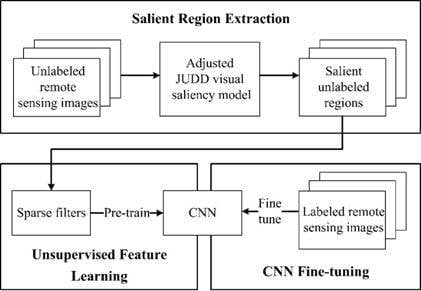
2. Methodology

The proposed method is composed of three stages: salient region extraction, unsupervised feature learning, and CNN fine-tuning (as shown in Figure 1). In the first stage, we employ an adjusted computational visual attention model, i.e., the visual saliency model proposed by Judd et al. (referred to as JUDD model in the rest of this paper) [17], to extract a great quantity of salient regions from unlabeled remote-sensing images. In the second stage, the salient regions are fed into sparse filters to learn favorable features for scene classification in an unsupervised manner. The learnt features are then used to assist the pre-training of a CNN through the initialization of its convolutional kernels using the parameters from the sparse filters. In the final stage, the pre-trained CNN is fine-tuned on a small amount of labeled remote-sensing images to further learn task-specific feature representation. To guarantee clarity, we adopt a self-designed demonstrative CNN architecture to demonstrate the whole methodology in this section.

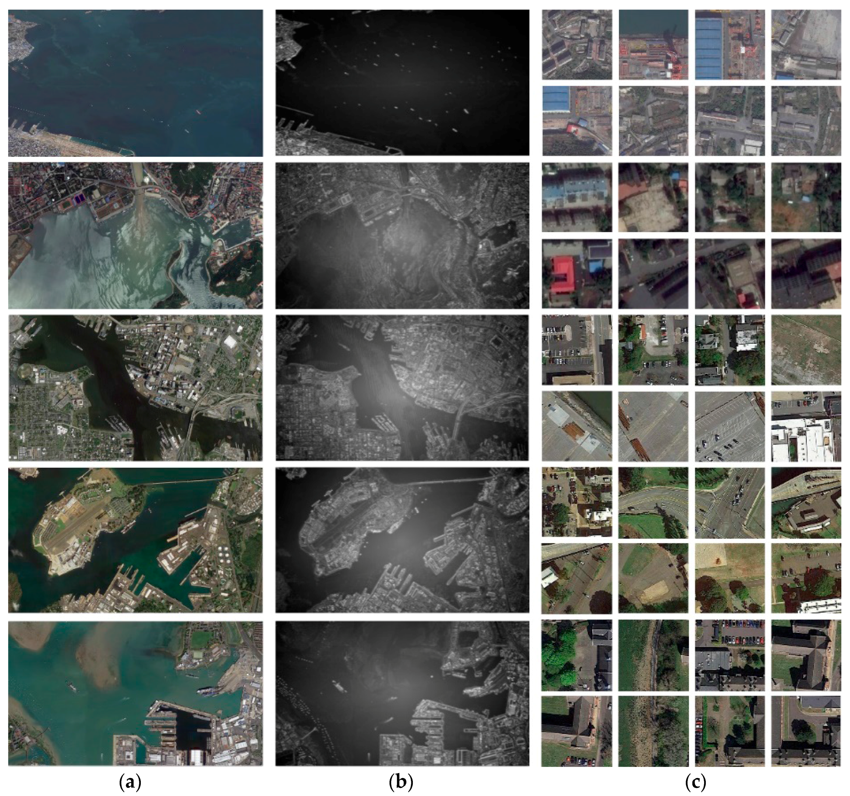
2.1. Salient Region Extraction

State-of-the-art unsupervised feature learning methods usually assign the same priority to all regions belonging to an image [18]. This strategy works fine for natural images because the meaningful objects usually occupy a large part of the natural images. In contrast, earth observation images usually contain lots of unvalued regions, such as sea and cloud, which are not regions-of-interest for most scene classification tasks. UL conducted on remote-sensing images must take the difference between the object and background into consideration, otherwise it is hard to learn task-specific features even with a large number of images. Thus, direct application of the existing UL methods to learn features from remote-sensing images will not only increase the problem complexity but also bring unnecessary calculation.

The human vision system (HVS) is challenged by a similar problem, capturing a huge amount of data every minute, from which humans can find meaningful patterns over time. Research into the HVS has found that it is often attracted to a handful of significant visual objects quickly in a complex scene and gives priority to the processing of these objects; the process being referred to as visual attention [19]. There is a clear application of visual attention to land-use scene classification: by determining image regions with the highest levels of visual attention, we can expect to greatly boost the performance and efficiency of scene classification using UL techniques.

While collecting human visual attention for a large number of images is infeasible, an alternative approach is to adopt computational visual models to mathematically determine the region-of-interest. Most computational visual attention models [20,21,22] are based on a bottom-up computation that does not consider top-down image semantics. The bottom-up computation tends to select regions with dramatic local variation as salient regions, which is not ideal for remote sensing images as there is no definite correspondence between regions with dramatic variation (e.g., sea surface with solar glint) and the region-of-interest. To extract more realistic salient regions from complex remote-sensing scenes, a model is needed that is consistent with a human’s perception. Considering that eye tracking data is the direct reflection of human visual attention, Judd et al. proposed a model composed of 33 low-, middle-, and high-level features learnt from a large database of eye tracking data [17]. The Judd saliency model is proven to be an effective biological model, predicting saliency of natural images that match those of a human with high consistency.

An obvious problem of domain transfer emerges when directly applying Judd’s model to the remote-sensing field because it is trained to predict a human’s attention for natural images. To solve this problem, this work utilizes a modification of Judd’s model to make it applicable to extracting salient regions from a remote-sensing image. Specifically, we select only the appropriate groups of features from the original ones contained in the Judd model. The selection is based on the analysis of whether the features are meaningful for describing the object-of-interest in remote-sensing images. For example, the group of features named ‘center prior’ is removed because remote-sensing images will not intentionally capture an object-of-interest near the center of the image. As a result, the following five groups of features are selected, whose detailed meaning can be found in Judd’s work [17].

• The local energy of the steerable pyramid filters;
• The saliency based on sub-band pyramids described by Torralba and Rosenholtz;
• Center-surrounded features in intensity, orientation, and color contrast calculated by Itti and Koch’s saliency method;
• The values and probabilities of each color channel;
• The probability of each color channel as computed from three-dimensional (3D) color histograms of the image filtered with a median filter at six different scales.

First, these features are adopted to extract saliency maps (shown in Figure 2b) from the original unlabeled remote-sensing images (shown in Figure 2a). Then, the saliency maps are evenly divided into patches with a size of 256 × 256 and the mean saliency of these patches is computed, on which basis the mean saliency of the whole image is calculated. Finally, those unlabeled patches whose saliency is larger than that of the whole image (shown in Figure 2c) are retained for further unsupervised feature learning.

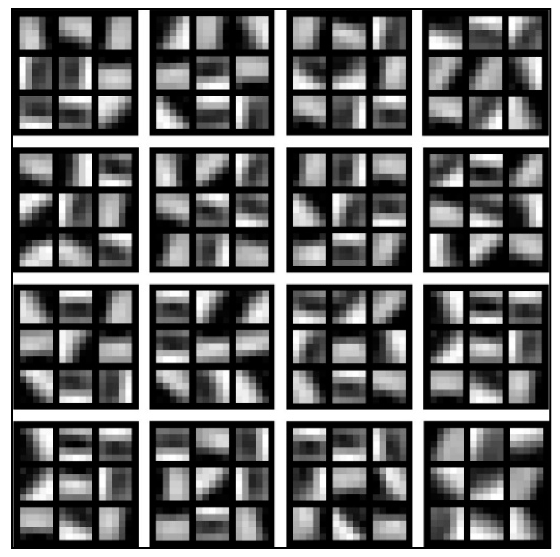
2.2. Unsupervised Feature Learning

After the salient regions are extracted from the unlabeled remote sensing images, sparse filters [15] are used to learn features from these salient regions. Sparse filtering is an unsupervised learning framework for sparse representation generation and is extremely simple to tune since it has only a single hyper-parameter to select. Furthermore, it scales very well with the dimension of the input, and more importantly, it was shown to achieve state-of-the-art performance on image recognition tasks. Sparse filters are based on the sparse theory, which indicates that a good feature distribution should satisfy three properties: population sparsity, i.e., each sample should be represented by only a few active features; lifetime sparsity, i.e., each feature should only be active for a few samples; and high dispersal, i.e., the distribution of each feature should have similar statistics and none of these features could be significantly more active than the others. However, these three properties are not isolated from each other: features that satisfy population sparsity and high dispersion also satisfy lifetime sparsity. Under the constraint of population sparsity, there should exist many non-active (zero) entries in the feature distribution matrix of the samples. Furthermore, under the constraint of high dispersion, these non-active entries should be approximately evenly distributed among all the features. Thus, each feature must have a significant number of non-active entries and be lifetime sparse. Taking the dependence into consideration, optimization in terms of both population sparsity and high dispersion is sufficient to learn sound representation.

Supposing we have a matrix X with domain R^O×M, symbolizing the original representation with M samples of dimensionality O. The high dispersion and population sparsity can be measured by Equations (1) and (2), respectively.

$${\mathbf{f}}_j=\frac{{\mathbf{f}}_j}{{\Vert {\mathbf{f}}_j\Vert }_2}$$

(1)

$${\Vert {\mathbf{f}}^{\left(i\right)}\Vert }_1={\Vert \frac{{\mathbf{f}}^{\left(i\right)}}{{\Vert {\mathbf{f}}^{\left(i\right)}\Vert }_2}\Vert }_1$$

(2)

where ${\mathrm{f}}_j^{(i)}=w_j{}^T{x}^{(i)}$ is the activity of feature j on example i and $x^{(i)}$ represents the ith sample. We simply first normalize the feature distribution matrix by rows, then by columns, and finally sum up the absolute value of all entries. Specifically, as Equation (1) shows, we first normalize each feature to be equally active by dividing each feature across all examples, then we normalize these features per example by computing Equation (2).

By applying Equations (1) and (2) successively, features are expected to be equally active and lie on the unit ${\ell }_2$-ball. For a dataset of M samples, the optimal features can be obtained by minimizing the object function shown by Equation (3).

$$min.{{\displaystyle \sum _{i=1}^M{\Vert {\mathbf{f}}^{\left(i\right)}\Vert }_1={\displaystyle \sum _{i=1}^M\Vert \frac{{\mathbf{f}}^{\left(i\right)}}{{\Vert {\mathbf{f}}^{\left(i\right)}\Vert }_2}\Vert }}}_1$$

(3)

After the sparse filters are learnt by greedy layer-wise training, they can be combined with a CNN to classify images, with the complete method being denoted the Saliency-guided Sparse Filter for Convolutional Neural Networks (SSF-CNN). Specifically, the filters of the CNN’s convolutional layers are substituted for the well-trained sparse filters. This substitution is based on the condition that sparse filters should generate a required number of filters with specified sizes according to the architecture of our CNN.

To preclude accuracy improvement introduced through elaborate CNN model design, we utilize a very simple CNN as shown in Figure 3 to demonstrate the effectiveness of SSF-CNN. This network is composed of nine layers, including a fully connected layer and four convolutional layers (C1~C4), each of which (except for C4) is followed by a max-pooling layer (S1~S3). K_i denotes the ith convolutional kernels replaced by the corresponding sparse filters. The numbers alongside K_i are the sizes and numbers of the pre-trained sparse filters. For instance, in the third convolutional layer, K₃ contains 16 groups of filters, and each group is composed of nine filters with the size of 5 × 5. Generally, the input of the CNN is a 100 × 100 × 3 image and the output is a 225-dimensional feature. The simplicity of the CNN lies in three aspects. First, the size of the input image is fixed to 100 × 100 × 3, which is smaller than the typical image size of state-of-the-art datasets. Second, instead of a successive decrease in the size of the convolutional kernels, the size is fixed to 5 × 5 in all convolutional layers. Finally, there is only one fully connected layer, whereas state-of-the-art CNN models have several.

For a dataset composed of M samples represented by N features, Equation (3) can be rephrased as Equations (4)–(6) when the CNN and sparse filters are combined:

$${\displaystyle \sum _{i=1}^M{\Vert {\mathbf{f}}^{\left(i\right)}\Vert }_1={\displaystyle \sum _{i=1}^M{\displaystyle \sum _{j=1}^N\frac{f_j^{(i)}}{C_i{D}_j}=}}}{\displaystyle \sum _{i=1}^M{\displaystyle \sum _{j=1}^N\frac{w_j{}^T{x}^{(i)}}{C_i{D}_j}}}$$

(4)

$$D_j={\Vert {\mathbf{f}}_j\Vert }_2=\sqrt{{\displaystyle \sum _{i=1}^M{\left(f_j^{(i)}\right)}^2}}$$

(5)

$$C_i={\Vert {\mathbf{f}}^{\left(i\right)}\Vert }_2=\sqrt{{\displaystyle \sum _{j=1}^N{\left(f_j^{(i)}\right)}^2}}$$

(6)

where the optimal w can be obtained by an off-the-shelf optimization package, e.g., a limited-memory Broyden–Fletcher–Goldfarb–Shanno algorithm (L-BFGS) represented as:

$$w=\mathrm{argmin}{\displaystyle \sum _{i=1}^M{\Vert {\mathbf{f}}^{\left(i\right)}\Vert }_1}.$$

(7)

In Figure 3, each input image or feature map is filtered by a series of filters in a convolutional layer whose kernels are derived from sparse filters. The learnt filters of K₃ are shown in Figure 4, which mainly characterize the edge and junction information in the images.

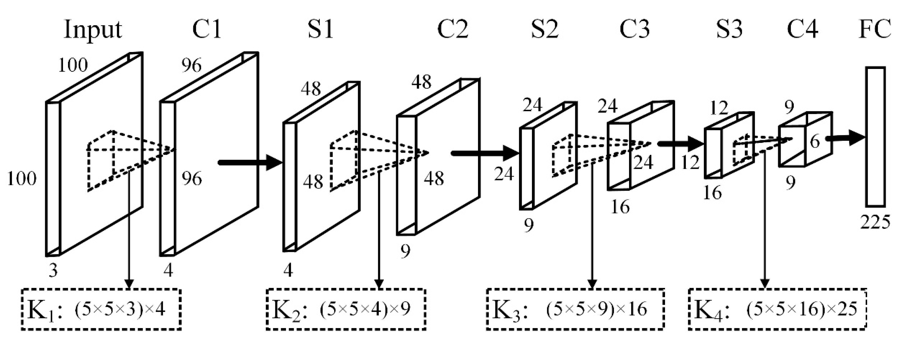
2.3. CNN Fine-Tuning

Until now, the pre-training of a CNN has been realized by the substitution of convolutional kernels with learnt sparse filters. The pre-trained CNN is able to offer informative features for discriminating unlabeled salient regions given by the Judd saliency model. However, differences between the source dataset (unlabeled images) and the target dataset (labeled scene images) still exist; therefore, the pre-trained CNN must be repurposed to the scene classification task. Specifically, a softmax classifier is added at the end of the CNN shown in Figure 3 to make predictions, whose number of neurons is equal to the desired number of categories. Following this, the CNN parameters are fine-tuned in a supervised manner using a stochastic gradient descent according to the categorical cross-entropy loss computed on a labeled dataset. With the learnt sparse filters K₁, K₂, K₃, and K₄, the convolutional process of a CNN can be described as:

$$y=g\left(g\left(g\left(g\left(g\left(x\times K_1+b_1\right)\times K_2+b_2\right)\times K_3+b_3\right)\times K_4+b_4\right)\times K_{fc}+b_{fc}\right)$$

(8)

where $\times$ denotes the convolutional computation of the filter with related feature maps, $g$ is the nonlinear operator, and $b_1$, $b_2$, $b_3$, and $b_4$ are the biases for each layer. $K_{fc}$ and $b_{fc}$ are the weights and biases in the fully connected layer, respectively, which are randomly initialized and gradually learnt through the fine-tuning process.

3. Experiment and Discussion

In this section, we first introduce the unlabeled and labeled remote-sensing image datasets that are used for unsupervised pre-training and supervised fine-tuning, respectively. Then, the experimental setup is described. After that, a validation experiment is designed to illustrate the effectiveness of the proposed method for scene classification. Then, our method is compared with the AlexNet model pre-trained on ImageNet to show the superiority of the proposed method. Finally, we compare the accuracy of our method with those obtained by state-of-the-art works.

3.1. Datasets

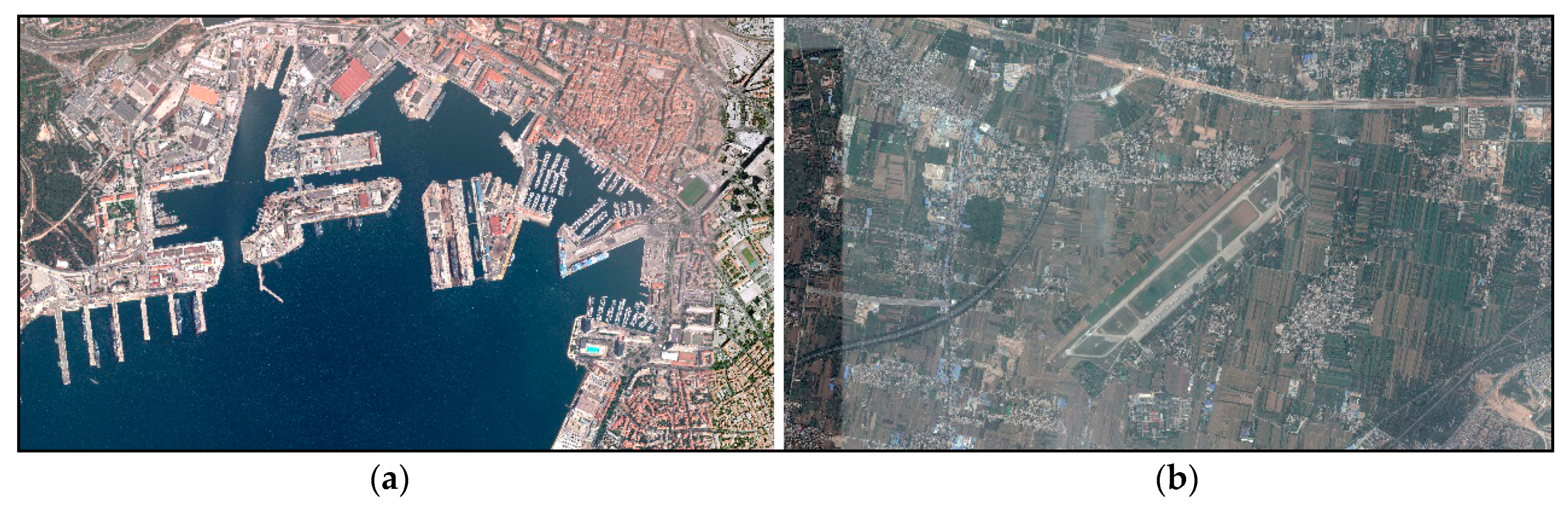
3.1.1. Unlabeled Dataset

To form the unlabeled dataset, 15 high-resolution remote-sensing images from GoogleEarth were collected. The sizes of these images range from 10,000 × 10,000 to 30,000 × 15,000. The images are divided into 32,954 patches with a size of 256 × 256 × 3, which are then fed into the Judd saliency model to automatically select salient patches for sparse filter learning. Sample images from the unlabeled dataset are shown in Figure 5.

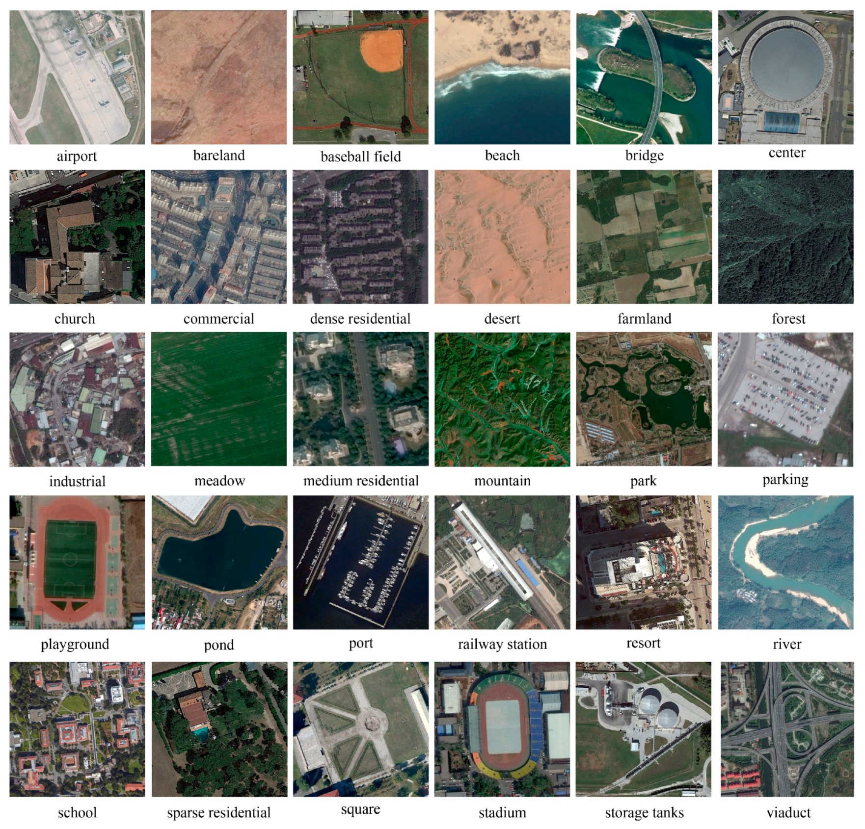
3.1.2. Labeled Datasets

In terms of the labeled dataset, two popular datasets—UCMerced [1] and AID [23]—are adopted. The UCMerced dataset covers 21 land-use categories, each of which contains 100 image patches with a size of 256 × 256 × 3. The AID dataset is composed of 10,000 image patches covering 30 land-use categories, each with a size of 600 × 600 × 3. The spatial resolution of images in UCMerced is fixed to 0.3 m, while the images in AID range between approximately 8 and 0.5 m. AID can be considered a more challenging dataset than UCMerced with higher intraclass variations, smaller interclass dissimilarity, and a larger relative scale. Sample images from the UCMerced and AID datasets are shown in Figure 6 and Figure 7, respectively.

3.2. Experimental Setup

To guarantee comparability between the accuracy of the proposed method and those reported in works presented in [2,3,5,7,8,9,10,11,12,13], the labeled dataset is divided into training and testing sets using a training–testing ratio of 80–20%, and five-fold cross validation is conducted. That is, the labeled image patches are almost equally divided into five non-overlapping groups randomly, with one group used as the testing set and the remaining four groups used as the training set in each fold. In each experiment, the CNN is used as a feature extractor, from which the output of the fully connected layer is extracted as image features, and a linear support vector machine (SVM) is adopted as the classifier. The results are reported in terms of mean overall accuracy and standard deviation among the five folds. To summarize the performances of the five folds, we also report the confusion matrix.

In terms of CNN hyperparameters selection, instead of adopting techniques such as random search and early stopping, we fix the learning rate and the number of training epochs empirically. This makes sense because the aim of this paper is to show the capacity of the proposed method to improve the land-use scene classification accuracy, and the fixed hyperparameters enable a fair comparison between different methods. However, it is likely that adopting advanced hyperparameter selection techniques would result in improved performance.

All experiments are conducted on a 64 bits Intel i7 6950X machine with 3.0 GHz of clock and 128 G of RAM memory. The graphics processing unit (GPU) used is a GeForce GTX1080Ti with 11 GB memory under CUDA version 7.5. The CNN is implemented in MatConvNet [24].

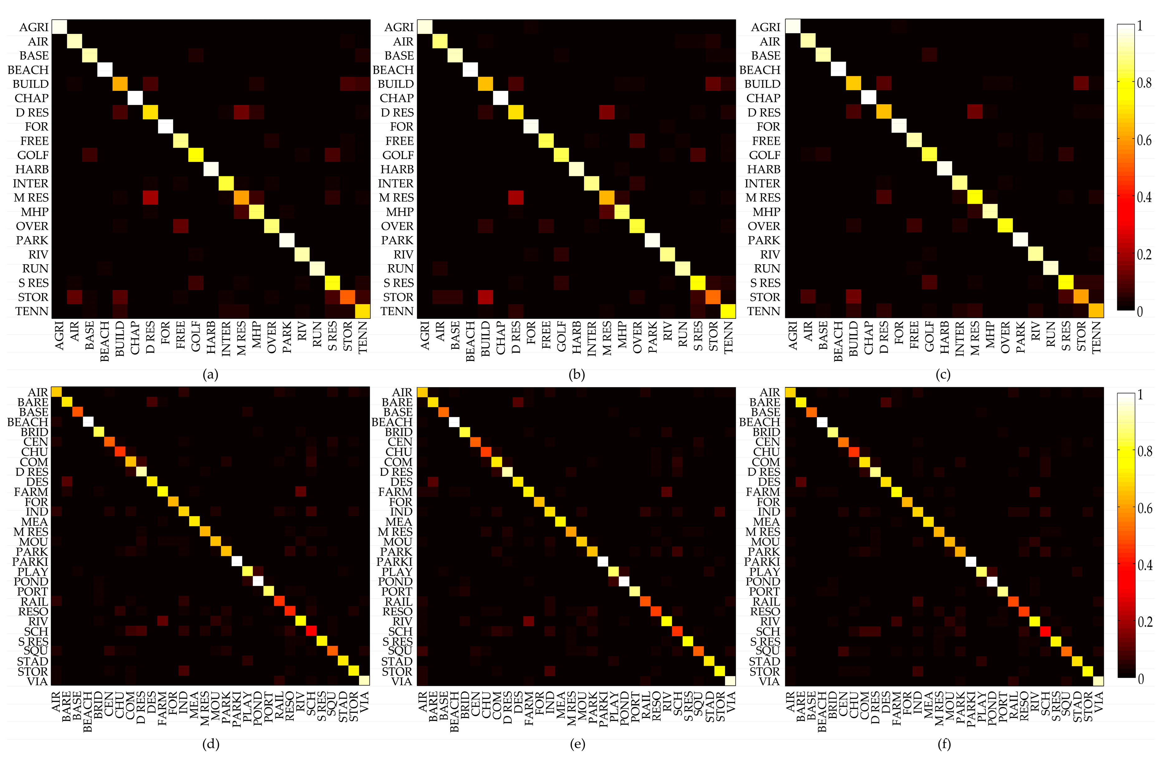
3.3. Validation of the Proposed Method

In the stage of salient region extraction, following the workflow described in Section 2.1, 18,358 salient patches with a size of 256 × 256 × 3 are selected from the 32,954 patches in the dataset. Thus, the sampling ratio is about 56%. In the stage of unsupervised feature learning, the off-the-shelf optimization package, L-BFGS, is used to optimize the objective function of sparse filters shown by Equation (3) until convergence.

To illustrate the performance of the proposed Saliency-guided Sparse Filter for Convolutional Neural Network (SSF-CNN) for scene classification in terms of both accuracy and efficiency, it is compared with two models, namely Plain-CNN and SF-CNN. Plain-CNN is trained from scratch using the labeled datasets, i.e., sparse filters are not adopted for CNN pre-training. SF-CNN adopts sparse filters to assist CNN pre-training as illustrated in Section 2.2, but the parameters of the sparse filters are learnt using all of the 32,954 patches. The comparison with Plain-CNN is designed to validate the necessity of UL, and the comparison with SF-CNN is designed to further validate the necessity of combining UL with a visual attention model.

Both Plain-CNN and SF-CNN have the same CNN architecture as shown in Figure 3, which is used to extract a feature vector of 255 dimensions from the fully connected layer, and a linear SVM is utilized to make predictions. The learning rates for fine-tuning are set to 0.0001 and the number of training epochs is set to 3000. The overall accuracies of Plain-CNN, SF-CNN, and SSF-CNN are shown in

Table 1. Overall accuracies of Plain-CNN, sparse filter (SF)-CNN, and saliency-guided sparse filter (SSF)-CNN on the UCMerced and AID datasets.

Labeled Dataset	Method	Overall Accuracy (%)
UCMerced	Plain-CNN	86.67 ± 1.50
	SF-CNN	87.52 ± 0.82
	SSF-CNN	88.91 ± 0.57
AID	Plain-CNN	78.95 ± 1.17
	SF-CNN	79.32 ± 1.04
	SSF-CNN	79.57 ± 0.91

, and the corresponding confusion matrices are shown in Figure 8.

From Table 1, it can be seen that for both the UCMerced and AID datasets, the SSF-CNN shows better accuracy, i.e., higher overall accuracy with lower standard derivation, than SF-CNN. Additionally, the Plain-CNN performs the poorest of all three CNNs. The superiority of both SSF-CNN and SF-CNN over Plain-CNN implies that sparse filtering is an effective UL method to pre-train the CNN, and thus can exploit the unlabeled data leading to better performance. Furthermore, the superiority of SSF-CNN over SF-CNN demonstrates the effectiveness of the saliency-guided method to obtain better feature representation, and in turn improve the performance. Specifically, when looking at the smaller training set, UCMerced (1680 images of 21 categories), SSF-CNN outperforms the Plain-CNN and the SF-CNN in terms of accuracy (about 1.1% higher). In contrast, looking at the larger training set, AID (8000 images of 30 categories), a trivial but consistent accuracy improvement (less than 0.4%) is observed. The reduction in accuracy improvement may be a result of the degradation in performance of UL methods when a large number of labeled images are introduced.

From Figure 8a–c, we can see that there are two major types of misclassification for the UCMerced dataset, i.e., the misclassification between ‘medium residential’ and ‘dense residential’ as well as the misclassification between ‘storage tanks’ and ‘buildings’. Those misclassifications by the Plain-CNN and SF-CNN are largely reduced by the SSF-CNN. For the AID dataset, the two major types of misclassification are mainly introduced by the confusion between ‘bareland’ and ‘desert’ as well as the confusion between ‘farmland’ and ‘river’. It should be noted that the misclassification may be partly attributed to the down-sampling of images from 600 × 600 to 100 × 100, which tends to suppress the detailed structure in the process of sparse filter learning.

It should be noted that although saliency-guided UL has been reported in the literature [13], the salient patches were actually extracted from labeled images, to which explicit semantic information had been attached. Thus, the work may have benefitted from the semantic information introduced by manual labeling because irrelevant background (such as the sea surface in Figure 5a) was selectively eliminated. On the contrary, in this paper, the salient regions are extracted from vast unlabeled images, which are completely free of hand-crafted or label-related semantic meaning. Furthermore, the salient regions in [13] are defined as patches that are distinctive with respect to their local and global surrounding, while the saliency in this paper is estimated by a computational visual attention model learnt from human eye tracking data. Thus, the extracted salient regions utilize the human vision system to find the meaningful patterns in satellite images and are therefore more consistent with human observation. It should be noted that random sampling is proven to outperform saliency-guided sampling at low sampling ratios [14], and they are comparative at a high sampling ratio. The novel unsupervised approach used in this work allows for a higher sampling ratio (up to about 56%), and thus provides sufficient training data for the saliency-guided sampling method (adopted by SSF-CNN) to outperform the random sampling method (adopted by SF-CNN).

To illustrate the efficiency of the proposed method, we also report the time consumed by the three main stages, i.e., salient region extraction, unsupervised feature learning, and CNN fine-tuning, of SSF-CNN on the UCMerced dataset in

Table 2. Time Consumed by SSF-CNN on the UCMerced Dataset.

Stage	Time (h)
Salient regions extraction	0.3
Unsupervised feature learning	55.2
CNN fine-tuning	12.1
Total	67.6

.

The SF-CNN needs 33.3 h more than SSF-CNN because SF-CNN has to use twice as many images to learn feature representation in the process of unsupervised feature learning, while SSF-CNN only focuses on the salient images. This illustrates that the proposed saliency-guided learning of sparse filters is more efficient than feature learning without guidance from saliency.

In summary, SSF-CNN can achieve a higher and more stable classification accuracy than SF-CNN and Plain-CNN. When the training set is small, SSF-CNN can also lead to a faster convergence speed. This shows a clear benefit in both unsupervised feature learning based on sparse filters as well as the saliency-guided patch extraction based on a visual attention model.

3.4. Comparison with AlexNet Pre-Trained on ImageNet

A common way to adapt CNNs pre-trained on large natural datasets to remote sensing land-use scene classification is to utilize labeled remote-sensing images for fine-tuning. In this method, the parameters of the CNN are initialized by a labeled dataset from a different field, e.g., ImageNet from computer vision. In our method, the convolutional parameters are initialized by an unlabeled dataset from the remote-sensing field, i.e., GoogleEarth images. It is interesting to compare the transfer learning method with our method.

A classical CNN architecture, i.e., AlexNet [25], is chosen as the CNN model for comparison. AlexNet consists of five convolutional layers, among which the first and second convolutional layers are followed by response normalization layers. Max-pooling layers follow both response normalization layers as well as the fifth convolutional layer. The remaining layers are three fully connected layers followed by a 1000-way softmax. The AlexNet model pre-trained on ImageNet is downloaded from the MatConvNet [24] website.

We make the comparison between the AlexNet model pre-trained on ImageNet (denoted by ImageNet-AlexNet) and the AlexNet model initialized using saliency-guided sparse filters (denoted by SSF-AlexNet) by fine tuning them on both the UCMerced and AID datasets. Specifically, the feature vector of 4096 dimensions is extracted from the last fully connected layer, and a linear SVM is adopted to make predictions. The learning rate of fine-tuning is set to 0.0001 and the number of training epochs is set to 1000 for an efficiency consideration. The overall accuracies of ImageNet-AlexNet and SSF-AlexNet on the UCMerced and AID datasets are shown in

Table 3. Overall Accuracies of ImageNet-AlexNet and SSF-AlexNet on the UCMerced and AID datasets.

Labeled Dataset	Method	Overall Accuracy (%)
UCMerced	ImageNet-AlexNet	94.29 ± 1.43
	SSF-AlexNet	92.43 ± 0.46
AID	ImageNet-AlexNet	91.66 ± 0.38
	SSF-AlexNet	88.71 ± 0.86

, and the corresponding confusion matrices are shown in Figure 9.

By comparing the results from Table 1 and Table 3, it can be seen that the accuracies obtained by SSF-AlexNet are higher than those obtained by the Plain-CNN by 5.76% and 9.14%, respectively, which indicates that our method can achieve higher accuracy when combined with more sophisticated CNN models. We have to admit that the feature representation obtained by the proposed method (SSF-AlexNet) is inferior to that transferred from supervised learning (ImageNet-AlexNet) by 2.4% in our experiments. We believe this is due to the tremendous scale difference between ImageNet (more than 14 million images) and our unlabeled dataset (18,358 images). However, two intrinsic advantages enable the proposed method to be a promising approach in land-use scene classification. On the one hand, pre-training on extremely large natural image datasets is much more time-consuming than the saliency-guided learning of sparse filters. The ImageNet training speed of AlexNet is 264.1 images/s [24], meaning that even though only 50% of the images of ImageNet are used as the training set, a single epoch can consume about 7.5 h. In contrast, the convolutional parameters of AlexNet can be initialized by the sparse filters in 55.8 h in our experiments. On the other hand, the proposed method frees researchers from constructing large labeled datasets adapted to the problem at hand. For example, there is no need to construct a large labeled dataset if we want to perform scene classification using SAR (synthetic aperture radar) or infrared imagery when we can instead initialize a CNN using unsupervised learnt sparse filters and then fine-tune it using a small labeled thermal infrared image dataset.

From Figure 9a,b, we can see that the most confusing land-use categories in the UCMerced dataset are ‘medium residential’ and ‘dense residential’. The confusion between storage tanks and buildings shown in Figure 8a–c has been suppressed greatly by ImageNet-AlexNet and SSF-AlexNet; however, the suppression by ImageNet-AlexNet is more obvious. In contrast, SSF-AlexNet performs better in discriminating ‘mobile home park’ from ‘dense residential’. Figure 9c,d shows that the misclassifications in the AID dataset are mainly due to the confusion between ‘park’ and ‘resort’ and the confusion between ‘industrial’ and ‘school’. The land-use scene misclassification observed here is different from the literature [23], where VGG-16 cannot discriminate ‘commercial’ from ‘school’ well. The performance difference may be related to the architectures of AlexNet and VGG-16.

3.5. Comparison with State-of-the-Art Research on the UCMerced Dataset

To illustrate the performance of SSF-CNN, we compare it with ten state-of-the-art research studies presented in [2,3,5,7,8,9,10,11,12,13] respectively. These studies are selected because all of them have been evaluated on the UCMerced dataset under the same training–testing ratio (80–20%). The overall accuracies obtained are shown in

Table 4. Comparison of State-of-the-Art Accuracies on the UCMerced dataset.

Method	Overall Accuracy (%)
SPCK++ [2]	77.38
OMP-k [7]	81.70
Saliency + SC [13]	82.72
Multilayer learning [10]	89.10
UFL-SC [8]	90.26
Partlets [3]	91.33
Multipath SC [11]	91.95
Quaternion + Q-OMP [9]	92.29
LGF [5]	95.48
Deconvolution + SPM [12]	95.71
SSF-CNN	88.91
SSF-AlexNet	92.43

.

Table 4 proves that SSF-CNN outperforms methods including SPM-BoVW, OMP-k, and Saliency + SC, and achieves comparable accuracy with multilayer learning. It should be noted that the CNN architecture of SSF-CNN is a demonstrative CNN model, in which the input image is resized to 100 × 100 and the filter size is fixed to 5 × 5. However, when using a more sophisticated CNN model, i.e., AlexNet, the proposed method is superior to most state-of-the-art methods except for LGF and Deconvolution + SPM. The results in Table 4 validate the proposed method as a promising supplement to CNN-based methods, and further accuracy improvements should be expected when more recent and sophisticated models, e.g., VGGNet, are combined with the proposed method.

4. Conclusions

This paper proposed a framework that improves the classification of land-use scenes with unsupervised feature learning on a large-scale unlabeled satellite imagery dataset. The paper is, we believe, very timely, in that it proposes a novel concept to improve classification by addressing the problem of a lack of large-scale labeled datasets in the land-use scene classification domain.

To our knowledge, our paper is the first one that learns the images’ representation on large-scale unlabeled satellite imagery datasets. Existing feature learning algorithms all conduct experiments on labeled datasets, and the data distribution of such datasets is not consistent with the large amount of unlabeled satellite imagery in real applications, which usually contain large amounts of meaningless area. To avoid extracting features from such meaningless areas, and to reduce unnecessary computation, our framework incorporates a computational visual attention model inspired by the human visual processing mechanism. The discriminative features learnt by sparse filters under the guidance of saliency are used to initialize the convolutional kernels of a CNN, which are further fine-tuned on a small number of labeled images.

Experiments are performed on the UCMerced and AID datasets, and the results show that the overall accuracy of our method with a demonstrative CNN architecture is 2.24% higher than that of Plain-CNN. Furthermore, with the more complex AlexNet architecture, our method achieved 92.43% overall accuracy, showing competitive results when compared with state-of-the-art land-use scene classification methods on the UCMerced dataset. The experiments’ results demonstrate that the proposed method can effectively improve CNN performance by taking advantage of easy-to-access unlabeled images.

The proposed framework has a wide range of potential applications, especially when large-scale labeled satellite images are not available, such as land-use scene classification on SAR or infrared imagery. It is also easy to integrate into some more sophisticated CNN-based deep learning models, e.g., VGGNet, to further improve their performances.

References

- Yang, Y.; Newsam, S. Bag-of-visual-words and spatial extensions for land-use classification. In Proceedings of the 18th ACM SIGSPATIAL International Symposium on Advances in Geographic Information Systems, San Jose, CA, USA, 2–5 November 2010; pp. 270–279. [Google Scholar]
- Yang, Y.; Newsam, S. Spatial pyramid co-occurrence for image classification. In Proceedings of the 2011 IEEE International Conference on Computer Vision, Barcelona, Spain, 6–13 November 2011; pp. 1465–1472. [Google Scholar]
- Cheng, G.; Han, J.; Guo, L.; Liu, Z.; Bu, S.; Ren, J. Effective and efficient midlevel visual elements-oriented land-use classification using VHR remote sensing images. IEEE Trans. Geosci. Remote Sens. 2015, 53, 4238–4249. [Google Scholar] [CrossRef]
- Risojevic, V.; Babic, Z. Fusion of global and local descriptors for remote sensing image classification. IEEE Geosci. Remote Sens. Lett. 2013, 10, 836–840. [Google Scholar] [CrossRef]
- Zou, J.; Li, W.; Chen, C.; Du, Q. Scene classification using local and global features with collaborative representation fusion. Inf. Sci. 2016, 348, 209–226. [Google Scholar] [CrossRef]
- Hinton, G.E.; Salakhutdinov, R.R. Reducing the dimensionality of data with neural networks. Science 2006, 313, 504–507. [Google Scholar] [CrossRef] [PubMed]
- Cheriyadat, A.M. Unsupervised feature learning for aerial scene classification. IEEE Trans. Geosci. Remote Sens. 2014, 52, 439–451. [Google Scholar] [CrossRef]
- Hu, F.; Xia, G.S.; Wang, Z.; Huang, X.; Zhang, L.; Sun, H. Unsupervised feature learning via spectral clustering of multidimensional patches for remotely sensed scene classification. IEEE J. Sel. Top. Appl. Earth Obs. Remote Sens. 2015, 8, 2015–2030. [Google Scholar] [CrossRef]
- Risojevic, V.; Babic, Z. Unsupervised quaternion feature learning for remote sensing image classification. IEEE J. Sel. Top. Appl. Earth Obs. Remote Sens. 2016, 9, 1521–1531. [Google Scholar] [CrossRef]
- Li, Y.; Tao, C.; Tan, Y.; Shang, K.; Tian, J. Unsupervised multilayer feature learning for satellite image scene classification. IEEE Geosci. Remote Sens. Lett. 2016, 13, 157–161. [Google Scholar] [CrossRef]
- Fan, J.; Chen, T.; Lu, S. Unsupervised feature learning for land-use scene recognition. IEEE Trans. Geosci. Remote Sens. 2017, 55, 2250–2261. [Google Scholar] [CrossRef]
- Lu, X.; Zheng, X.; Yuan, Y. Remote sensing scene classification by unsupervised representation learning. IEEE Trans. Geosci. Remote Sens. 2017, 55, 5148–5157. [Google Scholar] [CrossRef]
- Zhang, F.; Du, B.; Zhang, L. Saliency-guided unsupervised feature learning for scene classification. IEEE Trans. Geosci. Remote Sens. 2015, 53, 2175–2184. [Google Scholar] [CrossRef]
- Hu, J.; Xia, G.S.; Hu, F.; Zhang, L. A comparative study of sampling analysis in scene classification of high-resolution remote sensing imagery. Remote Sens. 2015, 7, 14988–15013. [Google Scholar] [CrossRef]
- Ngiam, J.; Pang, W.K.; Chen, Z.; Bhaskar, S.; Ng, A.Y. Sparse filtering. In Proceedings of the International Conference on Neural Information Processing Systems, Granada, Spain, 12–15 December 2011. [Google Scholar]
- Li, N.; Zhao, X.; Yang, Y.; Zou, X. Objects classification by learning-based visual saliency model and convolutional neural network. Comput. Intell. Neurosci. 2016, 2016. [Google Scholar] [CrossRef] [PubMed]
- Judd, T.; Ehinger, K.; Durand, F.; Torralba, A. Learning to predict where humans look. In Proceedings of the 2009 IEEE International Conference on Computer Vision, Kyoto, Japan, 29 September–2 October 2009; pp. 2106–2113. [Google Scholar]
- Bengio, Y.; Courville, A.C.; Vincent, P. Representation learning: A review and new perspectives. IEEE Trans. Pattern Anal. Mach. Intell. 2013, 35, 1798–1828. [Google Scholar] [CrossRef] [PubMed]
- Zhao, Q.; Koch, C. Learning saliency-based visual attention: A review. Signal Process. 2013, 93, 1401–1407. [Google Scholar] [CrossRef]
- Itti, L.; Koch, C. A saliency-based search mechanism for overt and covert shifts of visual attention. Vis. Res. 2000, 40, 1489–1506. [Google Scholar] [CrossRef]
- Hou, X.; Zhang, L. Saliency detection: A spectral residual approach. In Proceedings of the 2007 IEEE Conference on Computer Vision and Pattern Recognition, Minneapolis, MN, USA, 17–22 June 2007. [Google Scholar]
- Rosenholtz, R. A simple saliency model predicts a number of motion popout phenomena. Vis. Res. 1999, 39, 3157–3163. [Google Scholar] [CrossRef]
- Xia, G.S.; Hu, J.; Hu, F.; Shi, B.; Bai, X.; Zhong, Y.; Zhang, L.; Lu, X. AID: A benchmark data set for performance evaluation of aerial scene classification. IEEE Trans. Geosci. Remote Sens. 2016, 55, 3965–3981. [Google Scholar] [CrossRef]
- Vedeldi, A.; Lenc, K. MatConvNet: Convolutional neural networks for MATLAB. In Proceedings of the 23rd ACM International Conference on Multimedia, Brisbane, Australia, 26–30 October 2015. [Google Scholar]
- Krizhevsky, A.; Sutskever, I.; Hinton, G. ImageNet classification with deep convolutional neural networks. In Proceedings of the 25th International Conference on Neural Information Processing Systems, Lake Tahoe, NV, USA, 3–6 December 2012. [Google Scholar]