Directional ℓ₀ Sparse Modeling for Image Stripe Noise Removal

Abstract

Remote sensing images are often polluted by stripe noise, which leads to negative impact on visual performance. Thus, it is necessary to remove stripe noise for the subsequent applications, e.g., classification and target recognition. This paper commits to remove the stripe noise to enhance the visual quality of images, while preserving image details of stripe-free regions. Instead of solving the underlying image by variety of algorithms, we first estimate the stripe noise from the degraded images, then compute the final destriping image by the difference of the known stripe image and the estimated stripe noise. In this paper, we propose a non-convex ${\ell }_0$ sparse model for remote sensing image destriping by taking full consideration of the intrinsically directional and structural priors of stripe noise, and the locally continuous property of the underlying image as well. Moreover, the proposed non-convex model is solved by a proximal alternating direction method of multipliers (PADMM) based algorithm. In addition, we also give the corresponding theoretical analysis of the proposed algorithm. Extensive experimental results on simulated and real data demonstrate that the proposed method outperforms recent competitive destriping methods, both visually and quantitatively.

1. Introduction

Stripe noise (all denoted as “stripes” in this paper), which is generally caused by the inconsistency of the detecting element scanning or the influence of the detector moving and temperature changes, etc., is a universal phenomenon in remote sensing images. They may result in a bad influence not only on visual quality but also on subsequent applications in remote sensing images. Therefore, it is necessary to remove stripes and simultaneously maintain the healthy pixels from the degraded images. In general, the stripes have strongly directional and structural information, e.g., pixels normally damaged on row by row or column by column.

Recently, many approaches for destriping problems have been proposed, which may be roughly divided into three categories, mainly including filtering-based methods, statistics-based methods and optimization-based methods. Note that the proposed method belongs to the category of optimization-based methods.

The filtering-based methods, which generally obtain the results with variety of filters, have been widely utilized for remote sensing image destriping [1,2,3,4]. In Ref. [1], Chen et al. proposed an approach for remote sensing image destriping tasks based on a finite-impulse-response filter (FIR) in frequency domain. Although this method exhibits good results on the experimental CMODIS data, it inevitably leads to ringing and ripple artifacts. In Ref. [3], the wavelet analysis and adaptive Fourier zero-frequency amplitude normalization was used for hyperspectral image destriping problems, and this wavelet-based method had shown the promising ability for both stripes and random noise.

The statistics-based methods are mainly to analyze the distribution of stripes. These approaches have strong directional characteristic which is considered as the stripe prior for the remote sensing image destriping [5,6,7,8,9,10,11]. In Ref. [7], Weinreb et al. introduced a method based on matching empirical distribution functions (EDFs) for GOES-7 data, while the limitations and unstable property were caused by assuming the similarity and regularity among the stripes. To conquer the instability when the stripes are irregular or nonlinear, Rakwatin et al. [9] introduced a method, using both histogram-matching algorithm and local least squares fitting, to remove the stripes of Aqua MODIS band 6. In Ref. [10], spectral moment matching (SpcMM) method, which can automatically remove variety of frequencies stripes in a specific band, was proposed for Hyperion image destriping. In addition, Shen et al. [11] employed a piece-wise destriping method, which uses correction coefficients of each portion by considering neighboring normal row, for nonlinear and irregular stripes, but it cannot automatically select a threshold value to divide the image into different parts.

Recently, the optimization-based methods have shown superiorities for remote sensing image destriping problems [12,13,14,15,16,17,18,19,20,21,22,23]. The image destriping generally results in an ill-posed problem which fails to obtain a meaningful, stable and unique solution by the direct and traditional methods. Therefore, a common strategy for ill-posed problems is to construct a regularization model via investigating the priors of underlying image. For the optimization-based methods, they focus on searching and discovering the intrinsically prior knowledge to generate reasonable regularization models. In Ref. [24], Zorzi et al. proposed a sparse and low-rank decomposition for models specified in the time domain, and the authors in [25], proposed a sparse and low-rank decomposition of the inverse of the manifest spectral density to get a simpler graphical model. In Ref. [17], the authors presented a unidirectional total variational (UTV) model for MODIS (i.e., moderate-resolution imaging spectroradiometer) image stripes removal by fully considering the directional information of stripes. The UTV model is motivated by the classical TV model and the analysis of directional stripes. Chang et al. [21] proposed an optimization model combining the UTV with sparse priors of stripes applying to denoising and destriping simultaneously. In Ref. [22], the authors utilized the split Bregman iteration method with an anisotropic spectral-spatial total variation regularization to remove multispectral image stripes.

In summary, although these optimization-based methods can yield effective results of removing stripes, there still exists much room to improve. Most of them are implemented only from the perspective of noise removal, but without considering the typical properties of stripes, e.g., directional and structural properties. Even though they consider these properties, the formulated sparse destriping models fail to accurately depict the typical properties of stripes [26,27]. Moreover, the designed algorithms for non-convex models, e.g., ${\ell }_0$ sparse model, generally do not have the convergence analysis. These motivate us to develop a new model and design the corresponding effective algorithm, that theoretically guarantees the convergence, to solve the remote sensing destriping problems.

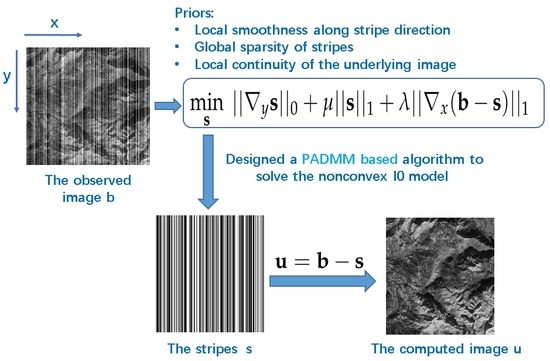
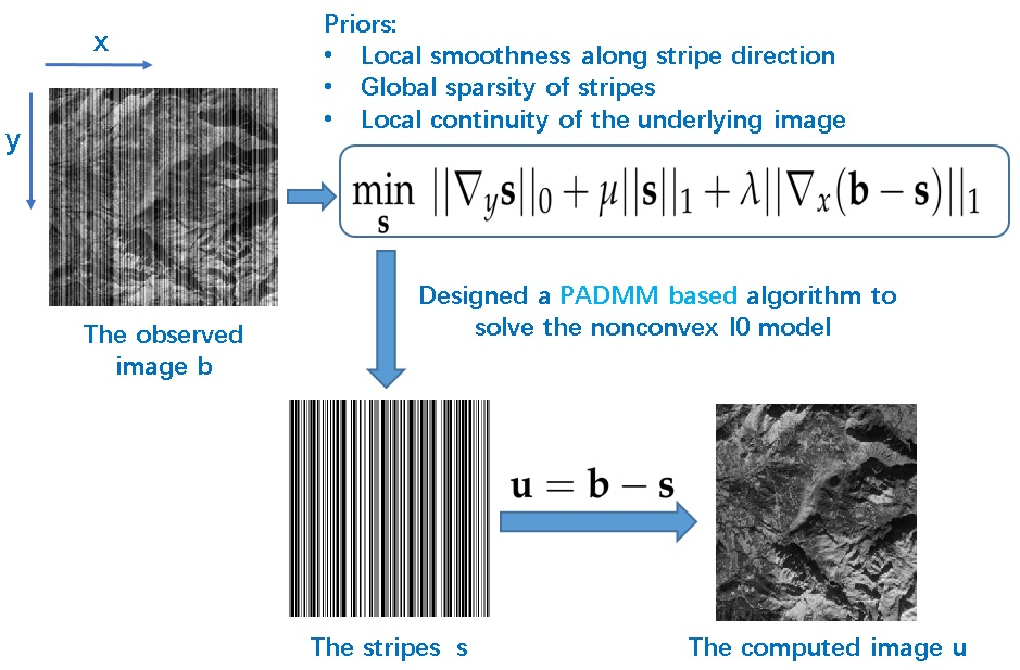
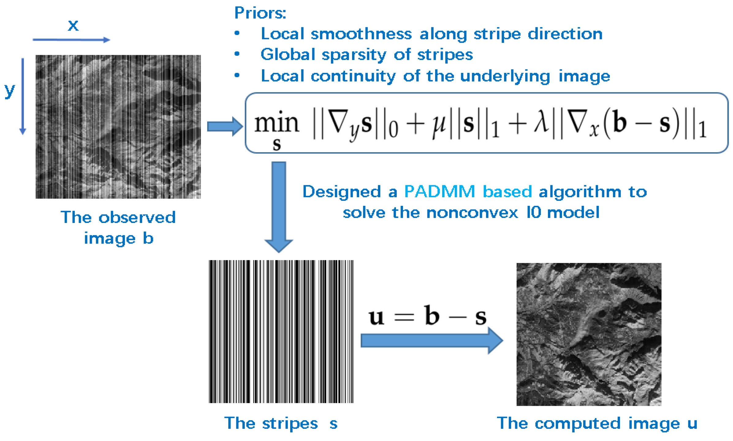
In this paper, to remove the stripes of remote sensing images, we propose a non-convex sparse model which mainly consists of three sparse priors, including an ${\ell }_0$ sparse prior by fully considering the directional property of stripes (y-axis), an ${\ell }_1$ sparse prior by considering the discontinuity of underlying image (x-axis), and the sparsity of stripes by considering the structural property of stripes. The framework of the proposed method is shown in Figure 1. Moreover, we design a proximal alternating direction method of multipliers (PADMM) based algorithm to solve the proposed non-convex sparse model. Actually, PADMM method mainly incorporates a proximal term into the well-known ADMM method which has been applied to many image processing applications, e.g., image deblurring [28], image denoising [29], tensor completion [30], etc. Note that, after adding this additional proximal term, the resulting algorithm is actually not an ADMM algorithm. The Karush–Kuhn–Tucker (KKT) conditions is the first-order necessary for a solution in nonlinear programming to be optimal. In particular, the convergence to the KKT point of the optimization problem is theoretically proven in the work.

The goal of this work is to propose a new model and design the corresponding effective algorithm for remote sensing image destriping, aiming to obtain promising results. The contributions of this work are summarized as follows

(1)

Fully considering the latent priors of stripes, we formulate an ${\ell }_0$ sparse model to depict the intrinsically sparse characteristic of the stripes.

(2)

We solve the non-convex model by a designed PADMM based algorithm which the corresponding theoretical analysis is given by this paper (see Appendix A).

(3)

The proposed method outperforms recent several competitive image destriping methods.

The outline of this paper is organized as follows. In Section 2, we will briefly introduce the related work. The proposed model and detailed solving algorithm will be shown in Section 3. In Section 4, we compare the proposed method with some competitive remote sensing image destriping methods, and give the discussions about the proposed method. Finally, conclusions are drawn in Section 5.

2. Related Work

2.1. Destriping Problem Formulation

The striping effects in remote sensing images mainly make up of additive and multiplicative components [15]. However, the multiplicative stripes can be described as additive case by the logarithm [31]. Thus, many types of research focus more on the additive stripes model

$$\mathbf{b}(x,y)=\mathbf{u}(x,y)+\mathbf{s}(x,y)$$

(1)

where $\mathbf{b}(x,y)$, $\mathbf{u}(x,y)$ and $\mathbf{s}(x,y)$ denote the components of the observed image, the underlying image and stripes at the location $(x,y)$, respectively. For convenience, a matrix-vector form can be written as follows

$$\mathbf{b}=\mathbf{u}+\mathbf{s},$$

(2)

where $\mathbf{b},\mathbf{u}$ and $\mathbf{s}\in {\mathbb{R}}^n$ represent the lexicographical order vectors of $\mathbf{b}(x,y)$, $\mathbf{u}(x,y)$ and $\mathbf{s}(x,y)$, respectively. The purpose of our work is to estimate the stripes $\mathbf{s}$, then the underlying image will be recovered by the formula of $\mathbf{u}=\mathbf{b}-\mathbf{s}$.

2.2. UTV for Remote Sensing Image Destriping

The total variation (TV) model, which is first proposed by Rudin, Osher, and Fatemi (ROF) [32], has shown powerful ability in many image applications, e.g., image unmixing [33], image deblurring [34], image inpainting [35], etc. It has the following form

$$E\left(\mathbf{u}\right)=\frac{1}{2}{\int }_{\Omega }{||\mathbf{u}-\mathbf{b}||}^2+\lambda TV\left(\mathbf{u}\right),$$

(3)

where $\lambda$ is a positive regularization parameter, and $TV\left(\mathbf{u}\right)$ represents the regularization expressed as

$$TV\left(u\right)={\int }_{\Omega }|\nabla \mathbf{u}|={\int }_{\Omega }\sqrt{{\left(\frac{\partial \mathbf{u}}{\partial x}\right)}^2+{\left(\frac{\partial \mathbf{u}}{\partial y}\right)}^2}dxdy.$$

(4)

In many approaches, $\mathbf{s}(x,y)$ is usually regarded as constant in a given line. Although this assumption has shown stability in MOS-B, it fails in MODIS. Not only predominant nonlinear effects, but also the data quality of random stripes have been obtained in many emissive bands. Thus, more realistic assumptions are introduced to design an efficient destriping method.

Without loss the generality, we can assume that the stripes are along the vertical direction (y-axis). In mathematical words, most pixels of the stripe noise $\mathbf{s}$ hold the following property [17]:

$$\left|\frac{\partial \mathbf{s}(x,y)}{\partial y}\right|\ll \left|\frac{\partial \mathbf{s}(x,y)}{\partial x}\right|,$$

(5)

where we denote y-axis is along stripes direction, and x-axis is across stripes direction. When $(x,y)$ is not the location of a pixel belonging to the stripes, both sides of Equation (5) are almost the same, denoted as

$$\left|\frac{\partial \mathbf{s}(x,y)}{\partial y}\right|\approx \left|\frac{\partial \mathbf{s}(x,y)}{\partial x}\right|.$$

(6)

By the relation in Equations (5) and (6), we get

$${\int }_{\Omega }\left|\frac{\partial \mathbf{s}(x,y)}{\partial y}\right|dxdy\ll {\int }_{\Omega }\left|\frac{\partial \mathbf{s}(x,y)}{\partial x}\right|dxdy,$$

(7)

which means

$$T{V}_y\left(\mathbf{s}\right)\ll T{V}_x\left(\mathbf{s}\right)$$

(8)

where $T{V}_x$ and $T{V}_y$ are horizontal and vertical variations, respectively. The authors in [17] encourage the robustness of stripes removal by minimizing the unidirectional total variation (UTV) model as follows

$$E\left(\mathbf{u}\right)=T{V}_y(\mathbf{u}-\mathbf{b})+\lambda T{V}_x\left(\mathbf{u}\right),$$

(9)

which can be solved by Euler–Lagrange equation based algorithm.

In Ref. [17], the UTV model can effectively deal with remote sensing image destriping problems, which has been demonstrated holding promising ability on Aqua and Terra MODIS data. Although TV model preserves image edges well, it can not accurately depict the specific directional property of stripes, and leads to undesired results. The UTV model that involves unidirectional constraint can remove stripes in the meanwhile not destroy the underlying image details. Inspired by the UTV model, we fully consider the intrinsically directional and structural priors of stripes and the continuous property of the underlying image. Finally, we form a unidirectional and sparsity-based optimization model.

3. The Proposed Method

Combining the stripes model in Equation (2), we will give the proposed optimal model with unidirectional prior motivated by the extension of the UTV model. In what follows, the detailed explanations of the proposed model and the corresponding solving algorithm will be exhibited.

Section 3.1 is the proposed model, Section 3.2 is the existing work, and Section 3.3 is the designed algorithm based on the existing work Section 3.2.

3.1. The Proposed Model

3.1.1. Local Smoothness Along Stripe Direction

The stripes of remote sensing images generally appear with column-by-column (y-axis) or row-by-row (x-axis). Without loss of generality, we view all stripes as column-by-column case to formulate the finally directional model (the row-by-row stripes can be easily rotated to column-by-column stripes to fit in the proposed model). Considering the smoothness of the stripes, the difference between adjacent pixels is quite small, or even close to zero, thus we generally use sparse prior to this character along the stripe direction (y-axis). The first regularization for the difference within the stripes is given as follows

$${\mathrm{R}}_1={||{\nabla }_y\mathbf{s}||}_0,$$

(10)

where ${\nabla }_y$ is a partial differential operator along stripe direction. We denote that ${\nabla }_y\mathbf{u}$ represents the vector form of ${\nabla }_y\mathbf{U}$ where $\mathbf{U}$ is a 2D image and the definition of ${\nabla }_x\mathbf{u}$ is similar to ${\nabla }_y\mathbf{u}$. Comparing with some popular sparse measures, e.g., ${\ell }_1$-norm and ${\ell }_p$-norm ($0<p<1$), the ${\ell }_0$-norm that stands for the number of non-zero elements of a vector is a promising measure to depict sparse property, thus here we employ ${\ell }_0$-norm to describe the sparsity of ${\nabla }_{y}s$. Although this term will lead to the non-convexity of the proposed model, we utilize the designed PADMM based algorithm to guarantee the solution converging to the KKT point.

3.1.2. Local Continuity of the Underlying Image

In general, the underlying image $\mathbf{u}$ along the x-axis is viewed as being continuous. When adding column-by-column stripes $\mathbf{s}$ to the underlying image, the local continuity of $\mathbf{u}$ is broken, which means that we should force ${\nabla }_x\mathbf{u}$ to be small to keep the continuity of $\mathbf{u}$. By this assumption and the relation $\mathbf{u}=\mathbf{b}-\mathbf{s}$, we utilize the following ${\ell }_1$-norm regularization to describe the local continuity of the underlying image

$${\mathrm{R}}_2={||{\nabla }_x(\mathbf{b}-\mathbf{s})||}_1,$$

(11)

where ${\nabla }_x$ represents the difference operator in the across-stripe direction. Note that this term is actually the second term of the UTV model in Equation (9).

3.1.3. Global Sparsity of Stripes

In many destriping approaches [26,27,36,37], the stripes can be naturally viewed as being sparse when the stripes are not dense. Here, we take the ${\ell }_1$-norm to depict the sparsity of stripes:

$${\mathrm{R}}_3={||\mathbf{s}||}_1.$$

(12)

Even though the stripes are dense, this sparse term in Equation (12) must be retained, since it can effectively avoid the undesired effect and keep the robustness of the proposed method (see more discussion in the Results Section).

Combining the above three regularization terms, we finally formulate the ${\ell }_0$ sparse model for remote sensing image destriping,

$$\underset{\mathbf{s}}{\min }{||{\nabla }_y\mathbf{s}||}_0+{\mu ||\mathbf{s}||}_1+\lambda {||{\nabla }_x(\mathbf{b}-\mathbf{s})||}_1,$$

(13)

where $\mu$ and $\lambda$ are two positive parameters.

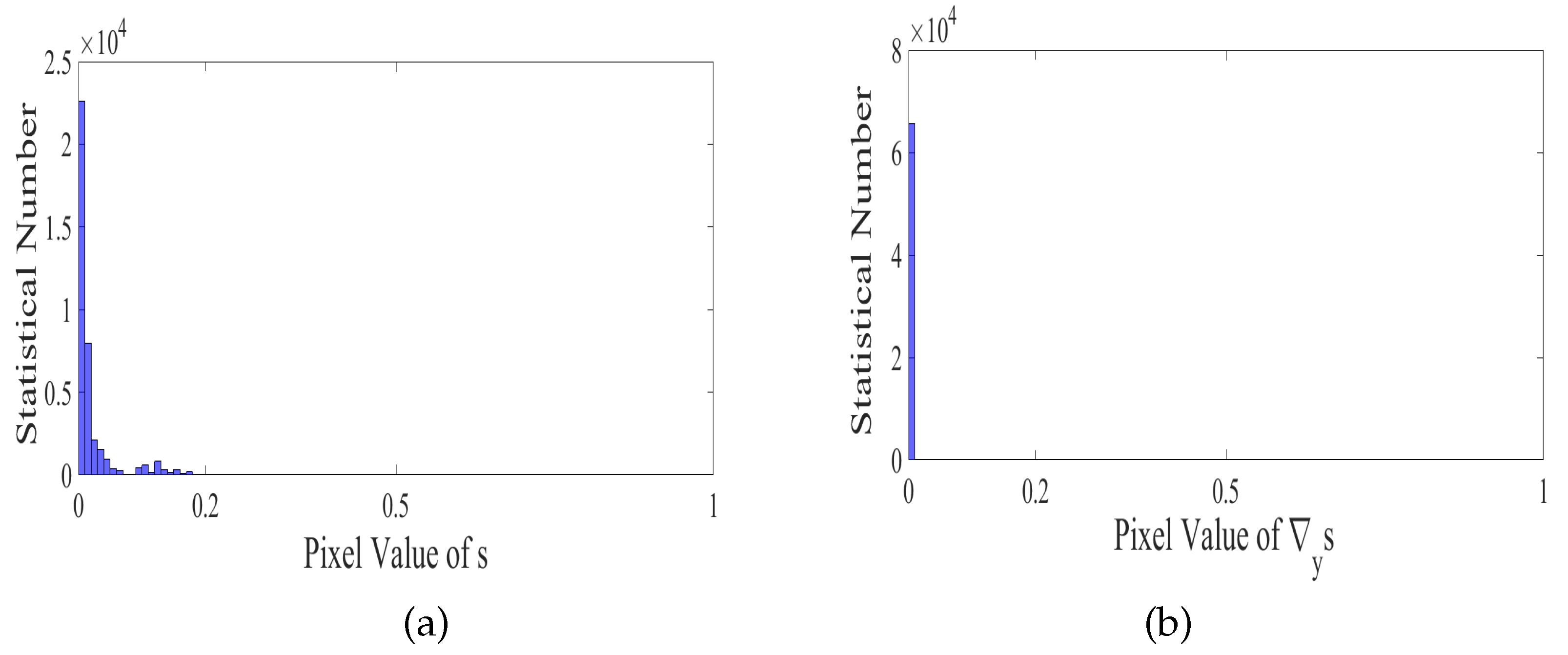
Note that the proposed model in Equation (13) is similar to the model in [26], since they both employ the directional property of stripes. However, there still exists an important difference that the model in [26] enforces ${\ell }_1$ norm to ${\nabla }_y\mathbf{s}$ and ${\ell }_0$ norm to $\mathbf{s}$ whereas our model enforces ${\ell }_1$ norm to s and ${\ell }_0$ norm to ${\nabla }_y\mathbf{s}$. From the experiment results, our optimal model can get better performance based on PADMM algorithm. For instance, Figure 2 shows the number of non-zero elements of $\mathbf{s}$ (Figure 2a) and ${\nabla }_y\mathbf{s}$ (Figure 2b), where $\mathbf{s}$ is estimated from a real image example by the method [26], it is clear that ${\nabla }_y\mathbf{s}$ is almost all around 0, whereas $\mathbf{s}$ is not. The ${\ell }_0$ norm is a promising way to depict sparsity, thus our model enforces ${\ell }_0$ norm to ${\nabla }_y\mathbf{s}$.

In what follows, we will exhibit how to solve the proposed non-convex sparse model by introducing the PADMM based algorithm, as well as give the theoretical analysis of the convergence.

3.2. The Solution

For the non-convex ${\ell }_0$ regularization term, there exist many approaches to approximate it, e.g., ${\ell }_1$-norm [38], the logarithm function [39] or the penalty decomposition algorithm (PDA) [40]. In this work, we first present a work in Lemma 1, i.e., the mathematical program with equilibrium constraints (MPEC) [36], to transfer the non-convex ${\ell }_0$ regularization term to the other equivalent one. Then, we can design a PADMM based algorithm to efficiently solve the equivalent model, in the meanwhile theoretically guarantee the convergence.

Lemma 1

(MPEC equation [36]). For any given $\mathbf{w}\in {\mathbb{R}}^n$, it holds that

$$\begin{array}{c}\hfill {||\mathbf{w}||}_0=\underset{\mathbf{0}\le \mathbf{v}\le \mathbf{1}}{\min }\langle \mathbf{1},\mathbf{1}-\mathbf{v}\rangle ,s.t.\mathbf{v}\odot |\mathbf{w}|=0,\end{array}$$

(14)

where $\langle \rangle$ represents the inner product of two vectors, and ⊙ denotes the elementwise product. The absolute of $\mathbf{w}$ stands for the absolute value of each element of $\mathbf{w}$. Then, ${\mathbf{v}}^{*}=\mathbf{1}-\mathit{sign}(|\mathbf{w}|)$ is the unique optimal solution of the minimization problem in Equation (14), and $\mathit{sign}(\mathrm{x})=\left\{\begin{array}{cc}1\hfill & \mathrm{x}>0\hfill \\ 0\hfill & \mathrm{x}=0\hfill \\ -1\hfill & \mathrm{x}<0\hfill \end{array}\right.$.

Proof. 

See details in [36]. ☐

From Lemma 1, the ${\ell }_0$-norm sparse optimization model in Equation (13) is equivalent to

$$\begin{array}{cc}\hfill \underset{\mathbf{0}\le \mathbf{v}\le \mathbf{1},\mathbf{s}}{\min }& \langle \mathbf{1},\mathbf{1}-\mathbf{v}\rangle +{\mu ||\mathbf{s}||}_1+\lambda {||{\nabla }_x(\mathbf{b}-\mathbf{s})||}_1,\hfill \\ \hfill s.t.& \mathbf{v}\odot |{\nabla }_y\mathbf{s}|=0,\hfill \end{array}$$

(15)

According to the analysis of [36], if ${\mathbf{s}}^{*}$ is the globally optimal solution of Equation (13), then $({\mathbf{s}}^{*},\mathbf{1}-\mathrm{sign}(|{\nabla }_y{\mathbf{s}}^{*}|\left)\right)$ is the unique global minimizer of Equation (15).

Note that Equation (15) is still a non-convex problem, and the non-convexity is only caused by the constraint $\mathbf{v}\odot |{\nabla }_y\mathbf{s}|=0$. However, the problem in Equation (15) is similar to the main problem in [36], which is efficiently solved by a PADMM based algorithm that theoretically guarantees the convergence. Therefore, we employ the designed PADMM based algorithm to solve the resulted problem in Equation (15), as well as give the theoretical analysis of the convergence.

In the following, we will use the PADMM based algorithm to solve the optimization problem in Equation(15).

3.3. PADMM Based Algorithm

Considering the non-smooth ${\ell }_1$ terms in the problem in Equation (15), we take the following variable substitutions to get the new optimization problem,

$$\begin{array}{cc}\underset{\mathbf{0}\le \mathbf{v}\le \mathbf{1},\mathbf{s},\mathbf{h},\mathbf{z},\mathbf{w}}{\min }\hfill & \langle \mathbf{1},\mathbf{1}-\mathbf{v}\rangle +{\mu ||\mathbf{z}||}_1+{\lambda ||\mathbf{w}||}_1,\hfill \\ s.t.\mathbf{v}\odot |\mathbf{h}|\hfill & =0,{\nabla }_y\mathbf{s}=\mathbf{h},\mathbf{s}=\mathbf{z},{\nabla }_x(\mathbf{b}-\mathbf{s})=\mathbf{w},\hfill \end{array}$$

(16)

with the auxiliary variables $\mathbf{h},\mathbf{z},\mathbf{w}\in {\mathbb{R}}^n$. The augmented Lagrangian function $\mathcal{L}$ of Equation (16) is as follows

$$\begin{array}{c}\mathcal{L}(\mathbf{h},\mathbf{z},\mathbf{w},\mathbf{v},\mathbf{s},{\mathit{\pi }}_{\mathbf{1}},{\mathit{\pi }}_2,{\mathit{\pi }}_3,{\mathit{\pi }}_4,{\beta }_1,{\beta }_2,{\beta }_3,{\beta }_4)\hfill \\ =\langle \mathbf{1},\mathbf{1}-\mathbf{v}\rangle +{\mu ||\mathbf{z}||}_1+{\lambda ||\mathbf{w}||}_1+\langle {\nabla }_y\mathbf{s}-\mathbf{h},{\mathit{\pi }}_1\rangle \hfill \\ +\frac{{\beta }_1}{2}{||{\nabla }_y\mathbf{s}-\mathbf{h}||}_2^2+\langle \mathbf{s}-\mathbf{z},{\mathit{\pi }}_2\rangle +\frac{{\beta }_2}{2}{||\mathbf{s}-\mathbf{z}||}_2^2\hfill \\ +\langle {\nabla }_x(\mathbf{b}-\mathbf{s})-\mathbf{w},{\mathit{\pi }}_3\rangle +\frac{{\beta }_3}{2}{||{\nabla }_x(\mathbf{b}-\mathbf{s})-\mathbf{w}||}_2^2\hfill \\ +\langle \mathbf{v}\odot |\mathbf{h}|,{\mathit{\pi }}_4\rangle +\frac{{\beta }_4}{2}{||\mathbf{v}\odot |\mathbf{h}|||}_2^2,\hfill \end{array}$$

(17)

where ${\mathit{\pi }}_1,{\mathit{\pi }}_2,{\mathit{\pi }}_3$, and ${\mathit{\pi }}_4$ are Lagrange multipliers, and ${\beta }_1,{\beta }_2,{\beta }_3$, and ${\beta }_4$ are positive parameters. The minimization problem in Equation (17) can be solved by the PADMM based algorithm. Next, we discuss the solution of each subproblem.

(1) The $\mathbf{h}$-subproblem can be written to the minimized problem as follows

$$\begin{array}{cc}\hfill \underset{\mathbf{h}}{\min }& \langle {\nabla }_y{\mathbf{s}}^k-\mathbf{h},{\mathit{\pi }}_1^k\rangle +\frac{{\beta }_1}{2}{||{\nabla }_y{\mathbf{s}}^k-\mathbf{h}||}_2^2\hfill \\ \hfill +& \langle {\mathbf{v}}^k\odot |\mathbf{h}|,{\mathit{\pi }}_4^k\rangle +\frac{{\beta }_4}{2}{||{\mathbf{v}}^k\odot |\mathbf{h}|||}_2^2.\hfill \end{array}$$

(18)

Now, let ${\mathrm{h}}_i$ is the i-th pixel of $\mathbf{h}$ and we discuss two situations when the element ${\mathrm{h}}_i\ne 0$, if ${\mathrm{h}}_i>0$,

$$\begin{array}{c}\hfill {\mathrm{h}}_i=\frac{({\beta }_1{\left({\nabla }_y\mathbf{s}\right)}_i+{\left({\mathit{\pi }}_1^k\right)}_i)-{\left({\mathit{\pi }}_4^k\right)}_i\odot {\left({\mathbf{v}}^k\right)}_i}{{\beta }_1+{\beta }_4{\left({\mathbf{v}}^k\right)}_i\odot {\left({\mathbf{v}}^k\right)}_i},\end{array}$$

(19)

if ${\mathrm{h}}_i<0$,

$$\begin{array}{c}\hfill {\mathrm{h}}_i=(-1)\frac{-({\beta }_1{\left({\nabla }_y{\mathbf{s}}^k\right)}_i+{\left({\mathit{\pi }}_1^k\right)}_i)-{\left({\mathit{\pi }}_4^k\right)}_i\odot {\left({\mathbf{v}}^k\right)}_i}{{\beta }_1+{\beta }_4{\left({\mathbf{v}}^k\right)}_i\odot {\left({\mathbf{v}}^k\right)}_i}.\end{array}$$

(20)

In summary, the $\mathbf{h}$-subproblem has the closed-form solution as follows

$$\begin{array}{c}\hfill {\mathbf{h}}^{k+1}=\mathrm{sign}\left({\mathbf{q}}^k\right)\ast \frac{|{\mathbf{q}}^k|-{\mathit{\pi }}_4^k\odot {\mathbf{v}}^k}{{\beta }_1+{\beta }_4{\mathbf{v}}^k\odot {\mathbf{v}}^k},\end{array}$$

(21)

where ${\mathbf{q}}^k={\beta }_1{\nabla }_y{\mathbf{s}}^k+{\mathit{\pi }}_1^k$.

(2) The $\mathbf{z}$-subproblem is given as follows

$$\begin{array}{c}\hfill \underset{\mathbf{z}}{\min }{\mu ||\mathbf{z}||}_1+\langle {\mathbf{s}}^k-\mathbf{z},{\mathit{\pi }}_2^k\rangle +\frac{{\beta }_2}{2}{||{\mathbf{s}}^k-\mathbf{z}||}_2^2,\end{array}$$

(22)

which has the closed-form solution by soft-thresholding strategy [41]

$$\begin{array}{c}\hfill {\mathbf{z}}^{k+1}=\mathbf{Shrink}({\mathbf{s}}^k+\frac{{\mathit{\pi }}_2^k}{{\beta }_2},\frac{\mu }{{\beta }_2}),\end{array}$$

(23)

where $\mathbf{Shrink}(\mathbf{a},\mathrm{T})=\mathrm{sign}\left(\mathbf{a}\right)\ast \max (|\mathbf{a}-\mathrm{T}|,0)$.

(3) Similar to $\mathbf{z}$-subproblem, $\mathbf{w}$-subproblem is written as follows

$$\begin{array}{c}\hfill \underset{\mathbf{w}}{\min }\lambda {||\mathbf{w}||}_1+\frac{{\beta }_3}{2}{||{\nabla }_x(\mathbf{b}-{\mathbf{s}}^k)-\mathbf{w}+\frac{{\mathit{\pi }}_3^k}{{\beta }_3}||}_2^2.\end{array}$$

(24)

The problem in Equation (24) has the following closed-form solution by the soft-shrinkage formulation,

$$\begin{array}{c}\hfill {\mathbf{w}}^{k+1}=\mathbf{Shrink}({\mathbf{p}}^k,\frac{\lambda }{{\beta }_3}),\end{array}$$

(25)

where ${\mathbf{p}}^k={\nabla }_x(\mathbf{b}-{\mathbf{s}}^k)+\frac{{\mathit{\pi }}_3^k}{{\beta }_3}$.

(4) The $\mathbf{v}$-subproblem can be written as follows

$$\begin{array}{c}\hfill \underset{\mathbf{0}\le \mathbf{v}\le \mathbf{1}}{\min }\langle \mathbf{v},{\mathbf{c}}^k\rangle +\frac{{\beta }_4}{2}{||\mathbf{v}\odot |{\mathbf{h}}^{k+1}|||}_2^2,\end{array}$$

(26)

where ${\mathbf{c}}^k=\mathbf{1}-{\mathit{\pi }}_4^k\odot |{\mathbf{h}}^{k+1}|$. Combining with the constraint $\mathbf{0}\le \mathbf{v}\le \mathbf{1}$, it has the closed-form solution,

$${\mathbf{v}}^{k+1}=\min (\mathbf{1},\max (\mathbf{0},\frac{-{\mathbf{c}}^k}{{\beta }_4|{\mathbf{h}}^{k+1}|\odot |{\mathbf{h}}^{k+1}|})).$$

(27)

(5) Here, PADMM based algorithm needs to introduce an extra convex proximal term $\frac{1}{2}{||\mathbf{s}-{\mathbf{s}}^k||}_{\mathbf{D}}^2$, which is defined as ${||\mathbf{x}||}_{\mathbf{D}}^2={\mathbf{x}}^{\mathbf{T}}\mathbf{Dx}$, and D is a symmetric positive definite matrix. The $\mathbf{s}$-subproblem becomes a strong convex optimization problem as

$$\begin{array}{cc}\underset{\mathbf{s}}{\min }\hfill & \langle {\nabla }_y\mathbf{s}-{\mathbf{h}}^{k+1},{\mathit{\pi }}_1^k\rangle +\frac{{\beta }_1}{2}{||{\nabla }_y\mathbf{s}-{\mathbf{h}}^{k+1}||}_2^2\hfill \\ & +\langle \mathbf{s}-{\mathbf{z}}^{k+1},{\mathit{\pi }}_2^k\rangle +\frac{{\beta }_2}{2}{||\mathbf{s}-{\mathbf{z}}^{k+1}||}_2^2\hfill \\ & +\langle {\nabla }_x(\mathbf{b}-\mathbf{s})-{\mathbf{w}}^{k+1},{\mathit{\pi }}_3^k\rangle \hfill \\ & +\frac{{\beta }_3}{2}{||{\nabla }_x(\mathbf{b}-\mathbf{s})-{\mathbf{w}}^{k+1}||}_2^2+\frac{1}{2}{||\mathbf{s}-{\mathbf{s}}^k||}_{\mathbf{D}}^2,\hfill \end{array}$$

(28)

where

$$\mathbf{D}=\frac{1}{\kappa }\mathbf{I}-({\beta }_1{\nabla }_y^T{\nabla }_y+{\beta }_2+{\beta }_3{\nabla }_x^T{\nabla }_x),$$

$$\kappa \in \left(0,\frac{1}{{\beta }_1{||{\nabla }_y||}_2^2+{\beta }_2+{\beta }_3{||{\nabla }_x||}_2^2}\right).$$

Then, Equation (28) will be equivalent to:

$$\begin{array}{c}\hfill {\mathbf{s}}^{k+1}=arg\underset{\mathbf{s}}{\min }\frac{1}{2}{||\mathbf{s}-{\mathbf{g}}^k||}_2^2,\end{array}$$

(29)

where ${\mathbf{g}}^k={\mathbf{s}}^k-\kappa [{\beta }_1({\nabla }_y{\mathbf{s}}^k-{\mathbf{h}}^{k+1})+{\beta }_2({\mathbf{s}}^k-{\mathbf{z}}^{k+1})-{\beta }_3{\nabla }_x^T({\nabla }_x\mathbf{b}-{\nabla }_x{\mathbf{s}}^k-{\mathbf{w}}^{k+1})]$.

(6) Finally, we update the Lagrangian multipliers by

$$\begin{array}{cc}\hfill {\mathit{\pi }}_1^{k+1}& ={\mathit{\pi }}_1^k+{\beta }_1({\nabla }_y{\mathbf{s}}^{k+1}-{\mathbf{h}}^{k+1}),\hfill \\ \hfill {\mathit{\pi }}_2^{k+1}& ={\mathit{\pi }}_2^k+{\beta }_2({\mathbf{s}}^{k+1}-{\mathbf{z}}^{k+1}),\hfill \\ \hfill {\mathit{\pi }}_3^{k+1}& ={\mathit{\pi }}_3^k+{\beta }_3({\nabla }_x(\mathbf{b}-{\mathbf{s}}^{k+1})-{\mathbf{w}}^{k+1}),\hfill \\ \hfill {\mathit{\pi }}_4^{k+1}& ={\mathit{\pi }}_4^k+{\beta }_4({\mathbf{v}}^{k+1}\odot |{\mathbf{h}}^{k+1}|).\hfill \end{array}$$

(30)

Combining Steps (1)–(6), we formulate the final algorithm to iteratively solve the proposed ${\ell }_0$ sparse model in Equation (13). In particular, the subproblems all have the closed-form solutions to ensure the accuracy of the algorithm. Finally, the solving process has been summarized in Algorithm 1.

In Algorithm 1, $\lambda$, $\mu$, ${\beta }_1$, ${\beta }_2$, ${\beta }_3$, and ${\beta }_4$ are some pre-defined parameters, while $tol$ and $M_{iter}$ represent the positive tolerance value and the maximum iterations, respectively. In this work, we set $tol=1/255$ and $M_{iter}={10}^3$. In the following, we discuss the convergence of Algorithm 1.

Algorithm 1 The algorithm for model in Equation (13)

Input: The observed image $\mathbf{b}$ (with stripes), the parameters $\lambda ,\mu ,{\beta }_i,i=1,2,3,4$,   the constant $\kappa \in (0,\frac{1}{{\beta }_1{||{\nabla }_y^T||}^2+{\beta }_2+{\beta }_3{||{\nabla }_x^T||}^2})$, the maximum number of iterations $M_{iter}$,   and the calculation accuracy $tol$. Output: The stripes $\mathbf{s}$ Initialize: (1) $k\leftarrow 0$, ${\mathbf{v}}^0\leftarrow \mathbf{1}$, ${\mathbf{s}}^0\leftarrow \mathbf{b}$, rho← 1 While rho> tol and k <$M_{iter}$ (2) $k\leftarrow k+1$ (3) Solve ${\mathbf{h}}^k$ by Equation (21) (4) Solve ${\mathbf{z}}^k$ by Equation (23) (5) Solve ${\mathbf{w}}^k$ by Equation (25) (6) Solve ${\mathbf{v}}^k$ by Equation (27) (7) Solve ${\mathbf{s}}^k$ by Equation (29) (8) Update the multipliers ${\mathit{\pi }}_i,i=1,2,3,4,$ by Equation (30) (9) Calculate   $rho={||{\nabla }_y{\mathbf{s}}^{k+1}-{\mathbf{h}}^{k+1}||}_2+{||{\mathbf{s}}^{k+1}-{\mathbf{z}}^{k+1}||}_2+{||{\nabla }_x(\mathbf{b}-{\mathbf{s}}^{k+1})-{\mathbf{w}}^{k+1}||}_2+{||{\mathbf{v}}^{k+1}\odot |{\mathbf{h}}^{k+1}|||}_2$. Endwhile

4. Experiment Results

In this section, we compare the proposed method with several competitive destriping methods, including the wavelet Fourier adaptive filter (WFAF) [3], the statistical linear destriping (SLD) [31], the unidirectional total variation model (UTV) [17], the global sparsity and local variational (GSLV) [26], and the Low-Rank Single-Image Decomposition (LRSID) [27], on both simulated and real remote sensing data. The codes of these methods, except the GSLV method, are available on the website (http://www.escience.cn/people/changyi/codes.html). Moreovre, we provide the code of the proposed method to compare the results on the website (http://www.escience.cn/people/dengliangjian/codes.html). As suggested in [27], we utilize the same periodic/nonperiodic stripes function adding stripes intensity [0, 255] to the underlying images. By the similar measure as in [27], the degraded images were normalized to [0, 1]. All experiments are conducted in MATLAB (R2016a) on a desktop with 16Gb RAM and Inter(R) Core(TM) CPU i5-4590: @3.30 GHz.

To evaluate the effects of different destriping methods, we will compare several qualitative and quantitative assessments. On the qualitative aspect, we show the visual results, the mean cross-track profile and the power spectrum of different methods. We also employ some acknowledged indexes, i.e., peak signal-to-noise ratio (PSNR) [42], structural similarity index (SSIM) [42], the inverse coefficient of variation (ICV) [15], mean relative deviation (MRD) [15], and the relative error (ReErr), to evaluate the performance of different approaches. These indexes are as follows,

$$\mathrm{PSNR}=10{\log }_{10}\frac{{255}^2\times n}{{||\widehat{\mathbf{u}}-\mathbf{u}||}^2},$$

where $\widehat{\mathbf{u}}$ and $\mathbf{u}$ are the estimated underlying image and the original underlying image. n represents the total number of pixels of one image.

$$\mathrm{SSIM}=\frac{(2{\mu }_x{\mu }_y+C_1)(2{\sigma }_{xy}+C_2)}{{\mu }_x^2+{\mu }_y^2+C_2},$$

where ${\mu }_x$ and ${\mu }_y$ represent the average value of x and y images. ${\sigma }_x$ and ${\sigma }_y$ stand for the variance of x and y images, and ${\sigma }_{xy}$ is the covariance of these two images. $C_1$ and $C_2$ are constant here.

$$\mathrm{ReErr}=\frac{{||{\mathbf{s}}_{added}-{\mathbf{s}}_{estimated}||}_2}{{||{\mathbf{s}}_{added}||}_2},$$

where the ${\mathbf{s}}_{added}$ and ${\mathbf{s}}_{estimated}$ represent the added stripes and estimated stripes by different methods, respectively.

$$\mathrm{ICV}=\frac{R_a}{R_{sd}},$$

where $R_a$ is the average value of the pixels with a window in a homogenous image region, and $R_b$ is the standard deviation of the pixels of the patch in this window. ICV calculates the homogeneous striped regions in estimated underlying image.

$$\mathrm{MRD}=\frac{1}{n}{\Sigma }_{i=1}^n\frac{|{\widehat{\mathbf{u}}}_i-{\mathbf{u}}_i|}{{\mathbf{u}}_i}\times 100\%,$$

where ${\widehat{\mathbf{u}}}_i$ is the estimated underlying image, and ${\mathbf{u}}_i$ is the original underlying image. MRD index shows the performance to retain the noise-free regions. Among these indices, ICV and MRD are non-reference indexes, and the others are full-reference indexes. Since stripes of the real images are dense, it is difficult to select several samples with the size of 10 × 10 window. In this paper, we select five different samples within a 6×6 window, and the mean ICV (MICV) and the mean MRD (MMRD) are shown in Table 4 for the six real experiments. Then, we will discuss how to select parameters. We note that we test the comparing methods according to the default or suggested parameters in their papers and codes.

4.1. Simulated Experiments

In simulated experiments, the stripes with periodic (Per) and nonperiodic (NonPer) noise are mainly determined by “Intensity” and r. Here, the “Intensity” means the added absolute value of the stripe scope, and the r represents the stripes ratio level within the remote sensing images. For convenience to compare, different stripes added to remote sensing images will be denoted as a vector with three elements, e.g., (Per, 10, 0.2) which represents the periodic stripes, the “Intensity” 10 and stripes ratio 0.2.

We take six experimental images, which the first and second are available on the website (“DigitalGlobe” with http://www.digitalglobe.com/product-samples), the sixth is available on the website (https://earthexplorer.usgs.gov/), and the second, fourth and fifth examples are available on the website (MODIS data with https://ladsweb.nascom.nasa.gov/), to test the performance of different methods. In the simulated experiments, the experimental images include: Washington DC Mall band 30, MODIS band 20, MODIS band 32, two small parts of the downloaded “Map Scale Ortho” image (“Map Scale Ortho” can be freely downloaded from the DigitalGlobe http://www.digitalglobe.com/resources/product-samples/30cm-imagery. We only use the two small parts of the downloaded “Map Scale Ortho” image acquired by the Satellite WorldView-3, since the “Map Scale Ortho” image is too large). To compare these methods clearly, we zoom in destriping details on the bottom left or bottom right of the image.

4.1.1. Periodic Stripes

For the periodic stripes case, we only take one example, i.e., the first column of Figure 3 with added stripes (Per, 10, 0.2), to compare the performance. Most of all existing methods performs quite effective to remove the stripes due to the simple structures of periodic stripes. The first column of Figure 3 also demonstrates the consistent conclusion that all comparing approaches remove the periodic stripes and well preserve the image details of stripe-free regions.

4.1.2. Nonperiodic Stripes

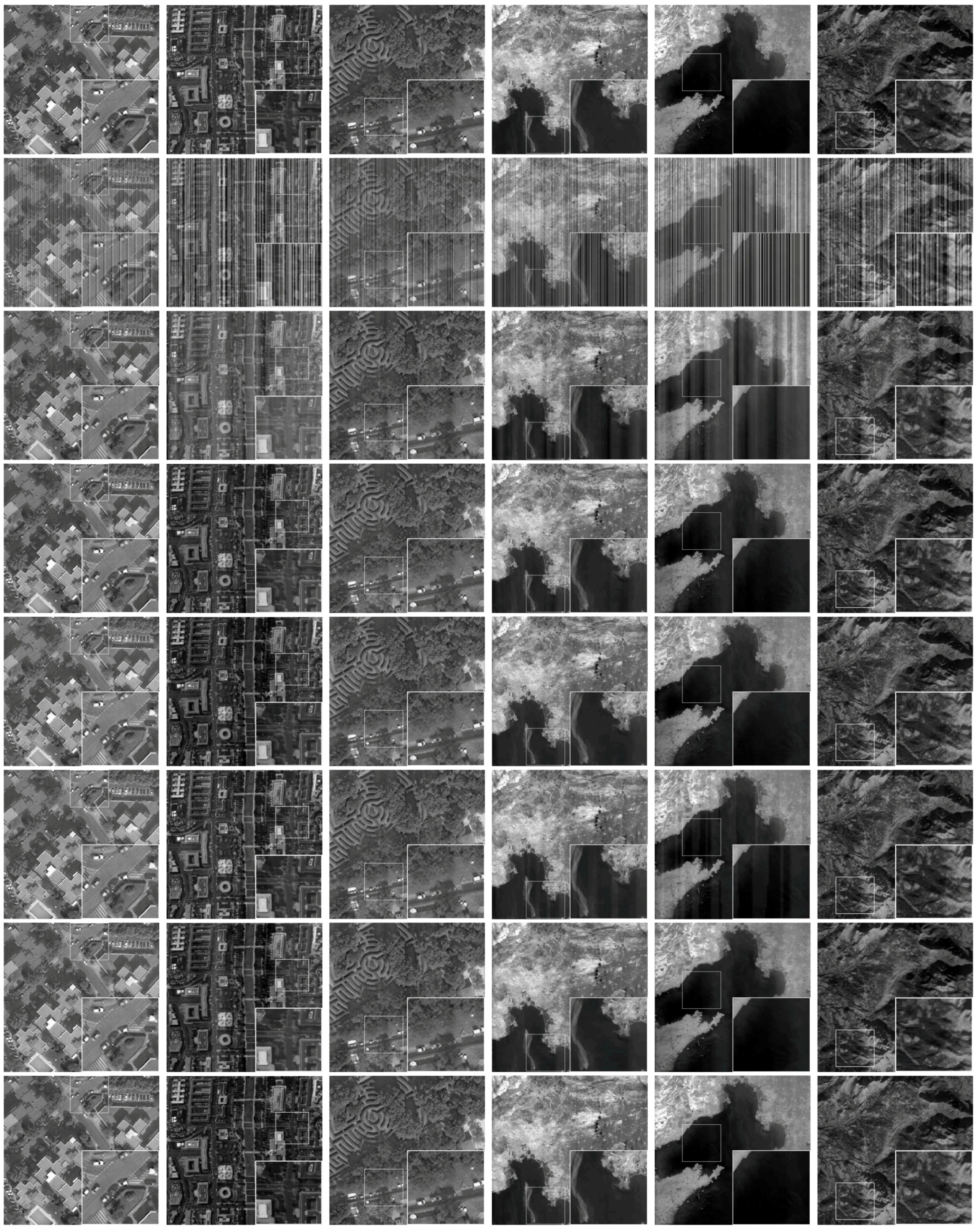
For the nonperiodic stripes case, we test five remote sensing images from the second column to the end column in Figure 3 with added stripes (NonPer, 100, 0.6), (NonPer, 50, 0.2), (NonPer, 60, 0.4), (NonPer, 100, 0.4) and (NonPer, 50, 0.6), respectively. Then, we display the destriping results of WFAF, SLD, UTV, GSLV, LRSID and the proposed method for different simulated remote sensing images starting from the third row to the end row. See the visual results of the second column, the WFAF method has an obvious black line and changes the intensity contrast of the underlying image. Although the other comparing methods can remove stripes, some regions change the intensity contrast of the underlying image on the left and the right parts, and the proposed method shows a good performance. Then, from the third to sixth examples, we can clearly observe the residual stripes and blurring effects resulted by the others comparing methods. Moreover, our method not only removes stripes completely but also preserves image details well. In Figure 4, we display the smaller patches of Figure 3 for visual quality comparisons, and our results have a better performance than the others.

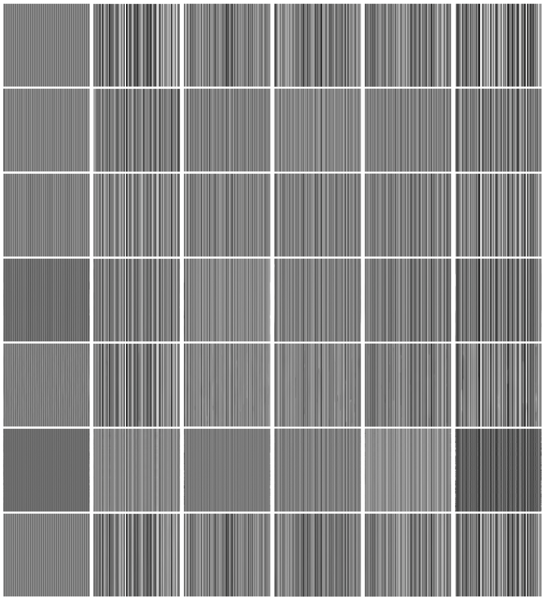
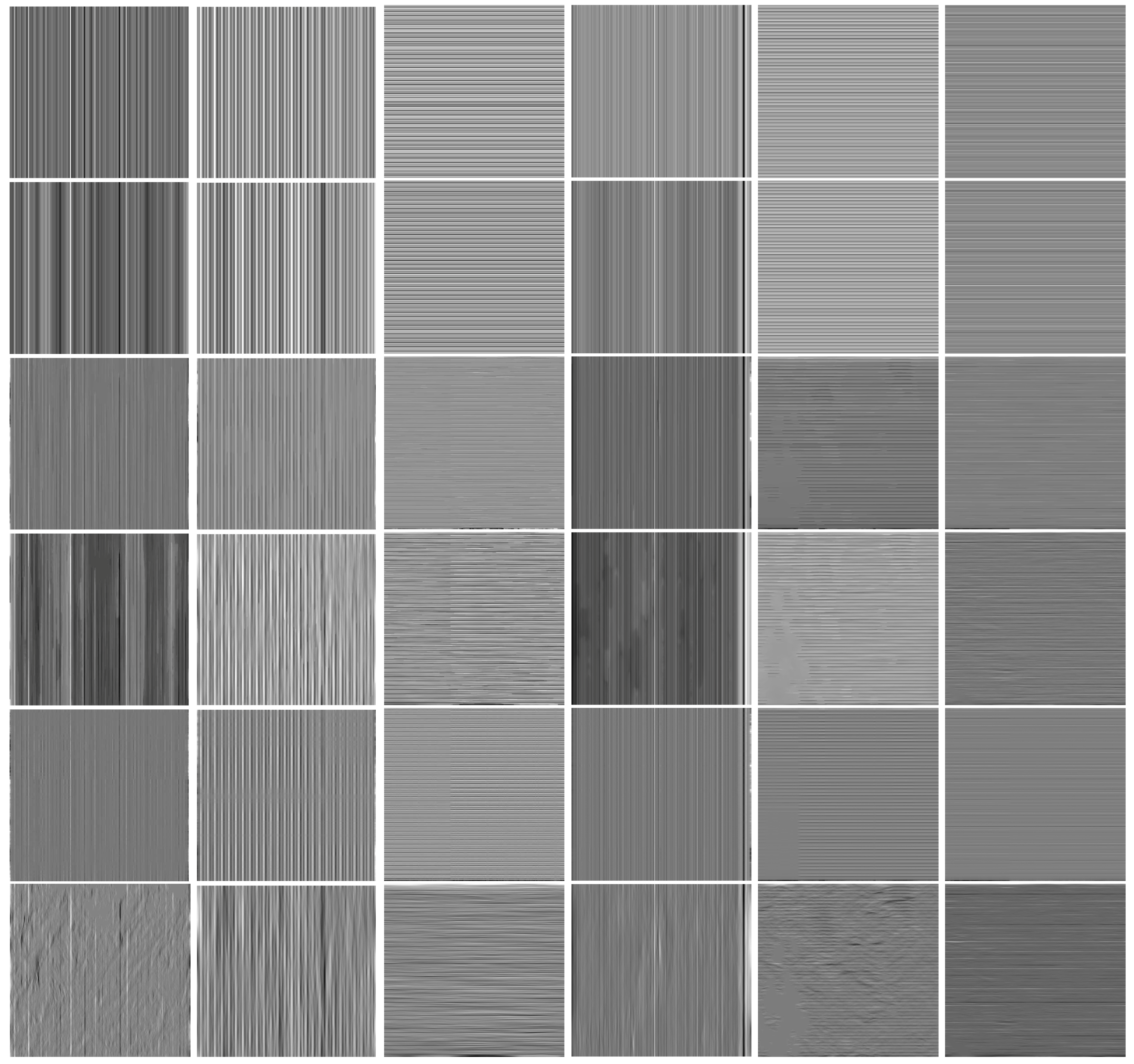
Figure 5 shows the estimated stripes based on Figure 3. In Figure 5, we can see that the other methods may generate blurring effect and change intensity contrast. Meanwhile, the estimated stripes of the proposed method neither eliminate image structures nor bring in blurring effects for both periodic and nonperiodic stripes cases.

In

Table 1. The ReErr results between ${\mathbf{s}}_{added}$ and ${\mathbf{s}}_{estimated}$, and the PSNR between the ground-truth and the computed image by the different methods.

	Images	(a)	(b)	(c)	(d)	(e)	(f)
ReErr	WFAF	0.1588	0.2828	0.2519	0.2468	0.2386	0.2574
	SLD	0.0874	0.1670	0.1723	0.1664	0.1330	0.1346
	UTV	0.0831	0.1542	0.2371	0.1818	0.1314	0.1375
	GSLV	0.0867	0.1030	0.2385	0.1926	0.0912	0.1654
	LRSID	0.0917	0.1884	0.2731	0.2125	0.1450	0.1897
	Ours	0.0193	0.0693	0.0365	0.0892	0.0304	0.0813
PSNR	WFAF	37.1239	21.3097	33.1166	28.6960	24.5539	28.1562
	SLD	42.3121	25.8878	36.4164	32.1200	29.6283	33.7867
	UTV	42.7463	26.5787	33.6413	31.3504	29.7370	33.6047
	GSLV	42.3798	30.0798	33.5899	30.8506	32.9031	31.9996
	LRSID	40.8345	24.7115	32.8728	30.4638	28.9817	31.6380
	Ours	55.4503	33.5287	49.8954	38.1697	42.4454	38.1677

, we show the ReErr results between the added stripes and estimated ones of Figure 5 from the quantitative aspect. Moreover, the PSNR values for different images have been shown in Table 1, and it is easy to know that our results outperform the other methods.

4.1.3. Averagely Quantitative Performance on 32 Test Images

To quantitatively test robustness and effectiveness of the proposed method,

Table 2. The mean value of PSNR and SSIM of 32 images with periodic noise.

	Intensity	Intensity = 10		Intensity = 50		Intensity = 100
	Ratio	r = 0.2	r = 0.6	r = 0.2	r = 0.6	r = 0.2	r = 0.6
PSNR	WFAF	41.400 ± 3.601	41.702 ± 3.870	37.160 ± 1.975	37.553 ± 1.975	32.196 ± 1.457	32.501 ± 1.732
	SLD	42.037 ± 2.927	41.048 ± 2.909	41.710 ± 2.930	41.957 ± 2.928	40.614 ± 2.549	41.644 ± 2.836
	UTV	42.030 ± 3.229	41.032 ± 2.886	40.920 ± 2.773	43.086 ± 2.298	41.470 ± 3.385	41.058 ± 3.299
	GSLV	42.552 ± 2.955	42.630 ± 2.886	42.202 ± 3.058	43.533 ± 2.856	43.431 ± 3.091	43.801 ± 2.705
	LRSID	43.948 ± 2.104	42.775 ± 2.010	42.308 ± 2.169	44.548 ± 1.976	43.779 ± 2.500	44.035 ± 2.014
	Ours	52.918 ± 4.074	49.497 ± 3.956	52.853 ± 4.910	49.212 ± 4.390	52.854 ± 4.902	49.182 ± 4.368
SSIM	WFAF	0.9934 ± 0.0058	0.9936 ± 0.0062	0.9887 ± 0.0084	0.9905 ± 0.0078	0.9818 ± 0.0103	0.9847 ± 0.0085
	SLD	0.9966 ± 0.0029	0.9966 ± 0.0029	0.9965 ± 0.0031	0.9965 ± 0.0032	0.9962 ± 0.0033	0.9964 ± 0.0037
	UTV	0.9959 ± 0.0027	0.9959 ± 0.0027	0.9911 ± 0.0025	0.9928 ± 0.0023	0.9954 ± 0.0024	0.9937 ± 0.0076
	GSLV	0.9991 ± 0.0077	0.9968 ± 0.0076	0.9916 ± 0.0079	0.9903 ± 0.0082	0.9966 ± 0.0085	0.9969 ± 0.0053
	LRSID	0.9990 ± 0.0107	0.9945 ± 0.0056	0.9932 ± 0.0044	0.9947 ± 0.0032	0.9936 ± 0.0047	0.9957 ± 0.0031
	Ours	0.9994 ± 0.0007	0.9987 ± 0.0011	0.9994 ± 0.0013	0.9986 ± 0.0016	0.9994 ± 0.0062	0.9986 ± 0.0019

and

Table 3. The mean value of PSNR and SSIM of 32 images with nonperiodic noise.

	Intensity	Intensity = 10		Intensity = 50		Intensity = 100
	Ratio	r = 0.2	r = 0.6	r = 0.2	r = 0.6	r = 0.2	r = 0.6
PSNR	WFAF	40.971 ± 2.523	39.372 ± 2.249	30.536 ± 1.508	37.609 ± 2.263	24.849 ± 1.573	22.594 ± 1.541
	SLD	41.476 ± 2.592	40.935 ± 2.201	35.964 ± 1.510	42.007 ± 3.020	30.963 ± 1.414	28.403 ± 1.729
	UTV	41.153 ± 2.880	38.615 ± 2.041	35.648 ± 1.527	42.505 ± 3.010	31.055 ± 4.687	31.599 ± 2.578
	GSLV	42.282 ± 2.359	39.018 ± 1.654	41.985 ± 1.239	39.838 ± 2.903	36.184 ± 1.399	35.408 ± 2.472
	LRSID	42.672 ± 1.418	39.034 ± 1.302	42.814 ± 1.349	40.497 ± 2.024	37.779 ± 1.212	33.559 ± 1.132
	Ours	48.801 ± 3.985	44.700 ± 3.784	49.057 ± 4.791	49.057 ± 4.492	44.365 ± 5.106	39.452 ± 4.494
SSIM	WFAF	0.9925 ± 0.0056	0.9903 ± 0.0069	0.9744 ± 0.0104	0.9905 ± 0.0081	0.9364 ± 0.0207	0.9029 ± 0.0565
	SLD	0.9965 ± 0.0031	0.9952 ± 0.0031	0.9950 ± 0.0041	0.9964 ± 0.0032	0.9907 ± 0.0060	0.9823 ± 0.0142
	UTV	0.9958 ± 0.0029	0.9934 ± 0.0052	0.9937 ± 0.0042	0.9914 ± 0.0056	0.9886 ± 0.0193	0.9851 ± 0.0122
	GSLV	0.9982 ± 0.0016	0.9917 ± 0.0042	0.9962 ± 0.0101	0.9967 ± 0.0088	0.9956 ± 0.0091	0.9933 ± 0.0152
	LRSID	0.9983 ± 0.0032	0.9934 ± 0.0113	0.9891 ± 0.0070	0.9962 ± 0.0042	0.9975 ± 0.0091	0.9924 ± 0.0402
	Ours	0.9991 ± 0.0006	0.9956 ± 0.0035	0.9990 ± 0.0010	0.9986 ± 0.0016	0.9979 ± 0.0012	0.9942 ± 0.0042

report the averagely quantitative comparisons of 32 remote sensing images, which are randomly selected from three websites (“DigitalGlobe” with http://www.digitalglobe.com/product-samples; some subimages of “hyperspectral image of Washington DC Mall” with https://engineering.purdue.edu/~biehl/MultiSpec/; “MODIS” data with https://ladsweb.nascom.nasa.gov/). In the tables, the best PSNR and SSIM results have been highlighted in bold. Especially, we compare these methods on 32 remote sensing images with fixed parameters for each method.

Table 2 shows the PSNR and SSIM results on periodic stripes with different stripe levels. Although variance of PSNR is not the smallest, the SSIM of the proposed method holds the best performance, and SSIM is an important index to indicate stability on structural similarity of one method. Therefore, the proposed method can improve the PSNR and SSIM results to remove stripes.

For the nonperiodic stripes, we show the mean value results in Table 3. The WFAF method shows the instability, and the PSNR and SSIM of LRSID method are consistent with the results in [27]. From the two tables, our method always shows a good performance.

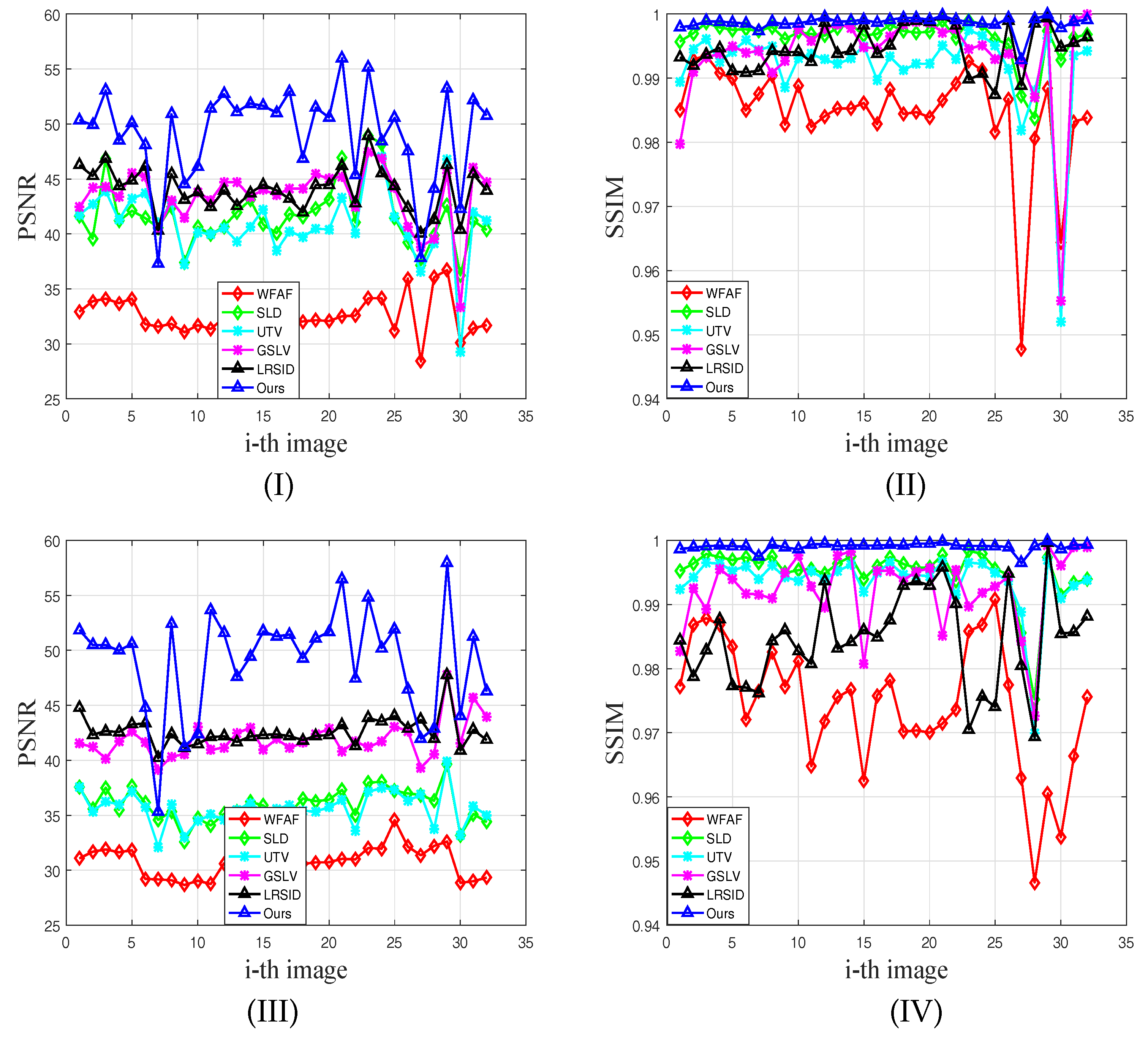
In Figure 6, we take two examples of Table 2 to show the PSNR and SSIM performance of all comparing methods on each image. The y-axis stands for the value of PSNR or SSIM and the x-axis represents the i-th image of 32 examples. Figure 6I,II show the PSNR and SSIM performance of stripes (Per, 100, 0.6). Moreover, Figure 6III,IV show that of stripes (NonPer, 50, 0.2). Although the PSNR results fluctuate with respect to different images, our method holds the best PSNR results on most of all images. Moreover, the SSIM results show the best performance with the smallest variance, which is consistent with the results of Table 2 and Table 3. From Figure 6, our method is superior to the other comparing methods.

4.2. Real Experiments

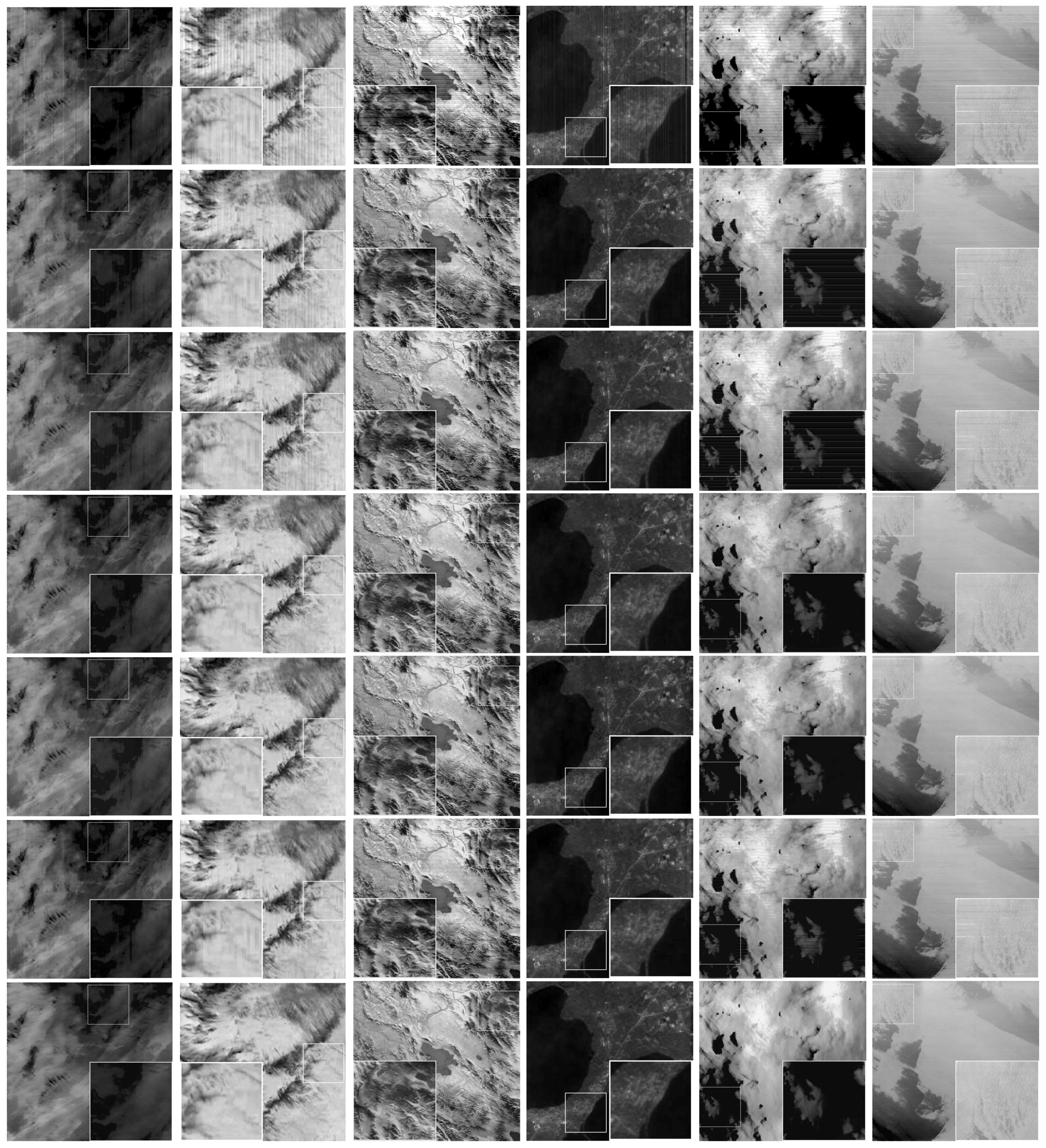
We also display the destriping results of six methods for six real remote sensing images, which are also available on the website (https://ladsweb.nascom.nasa.gov/) (see Figure 7). In the real experiments, we show the six real images: MODIS band 34, original band 28, Original Aqua MODIS band 30, MODIS band 136, Original MODIS Terra band 27, and Terra Africa MODIS band 33. Similar to Figure 3, the six real images with different stripes are shown in the first row, and the destriping results of all comparing methods are presented from the second row to the end row.

In Figure 8, we show the extracted stripe components of compared methods for the six real images in Figure 7. It seems that the proposed method removes too much background information in the real image experiments. Moreover, the non-reference indexes of MICV and MMRD have been shown in

Table 4. The MICV and MMRD index results of the six real images.

	Images	Index	WFAF	SLD	UTV	GSLV	LRSID	Ours
	(a)	MICV	4.7759	4.9274	6.8851	5.3955	7.4612	5.4162
		MMRD (%)	0.0078	0.0446	0.1646	0.1199	0.1590	0.0945
	(b)	MICV	5.5871	5.5740	8.9350	6.4436	7.5592	7.4144
		MMRD (%)	0.0405	0.0377	0.1142	0.0695	0.0900	0.0662
	(c)	MICV	3.9619	3.9940	4.3038	4.2884	4.0437	4.9604
		MMRD (%)	0.0286	0.0271	0.0276	0.0258	0.0385	0.0243
	(d)	MICV	1.7057	1.6720	3.2297	2.2237	3.5039	2.6574
		MMRD (%)	0.3600	0.3785	0.1707	0.0876	0.2250	0.0262
	(e)	MICV	0.8673	0.8533	0.8849	0.8786	0.8955	0.9017
		MMRD (%)	0.0328	0.0311	0.0432	0.0312	0.0265	0.0264
	(f)	MICV	13.5619	13.2952	16.1001	16.5111	13.6906	16.7897
		MMRD (%)	0.0196	0.0210	0.0214	0.0190	0.0250	0.0176

, and the best results have been highlighted. The proposed method shows a good performance in most of the cases. Although the results of the first two images are not the best, the results have only little difference among these compared methods. The indexes of MICV and MMRD depend on the selected patches and the window size. Different selected patches and window size may result in the performance of the two indexes. Here, we utilize them to partially evaluate the quantitative performance of the real image destriping.

In Figure 7, for the first, fifth and last real images, the proposed method not only removes the stripes completely, but also preserves image details on stripe-free regions well. Note that the methods GSLV and LRSID fail to obtain desired results for the first image as the mentioned in their papers. For the fourth column, there are also several stripe residuals with WFAF and SLD, and the wide black shadow areas appear by the UTV, GSLV and LRSID methods. Moreover, the destriping results of the WFAF and SLD leave obvious stripes for the second image, and still exist the wispy stripes for the third example. According to several real experiments, the results demonstrate the universal effectiveness and stability of the proposed method.

4.3. More Analysis

4.3.1. Qualitative Analysis

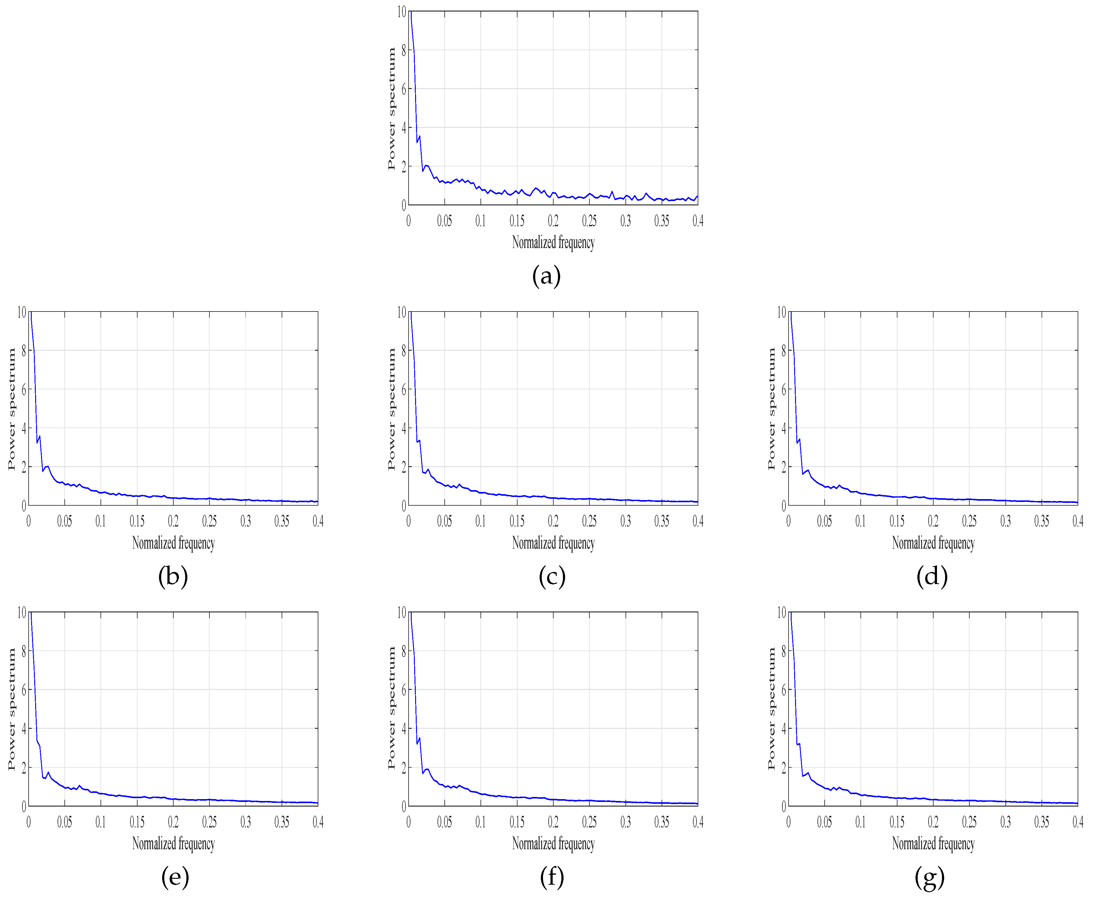
For the further comparisons of different destriping methods for simulated and real remote sensing images, we show the following two assessments. One is the mean cross-track profile that the x-axis stands for the column number of an image and the y-axis represents the mean value of each column (see Figure 9 and Figure 10). The other is the power spectrum that the x-axis is the normalized frequencies of an image, and the y-axis shows the spectral magnitude with a logarithmic scale (see Figure 11 and Figure 12).

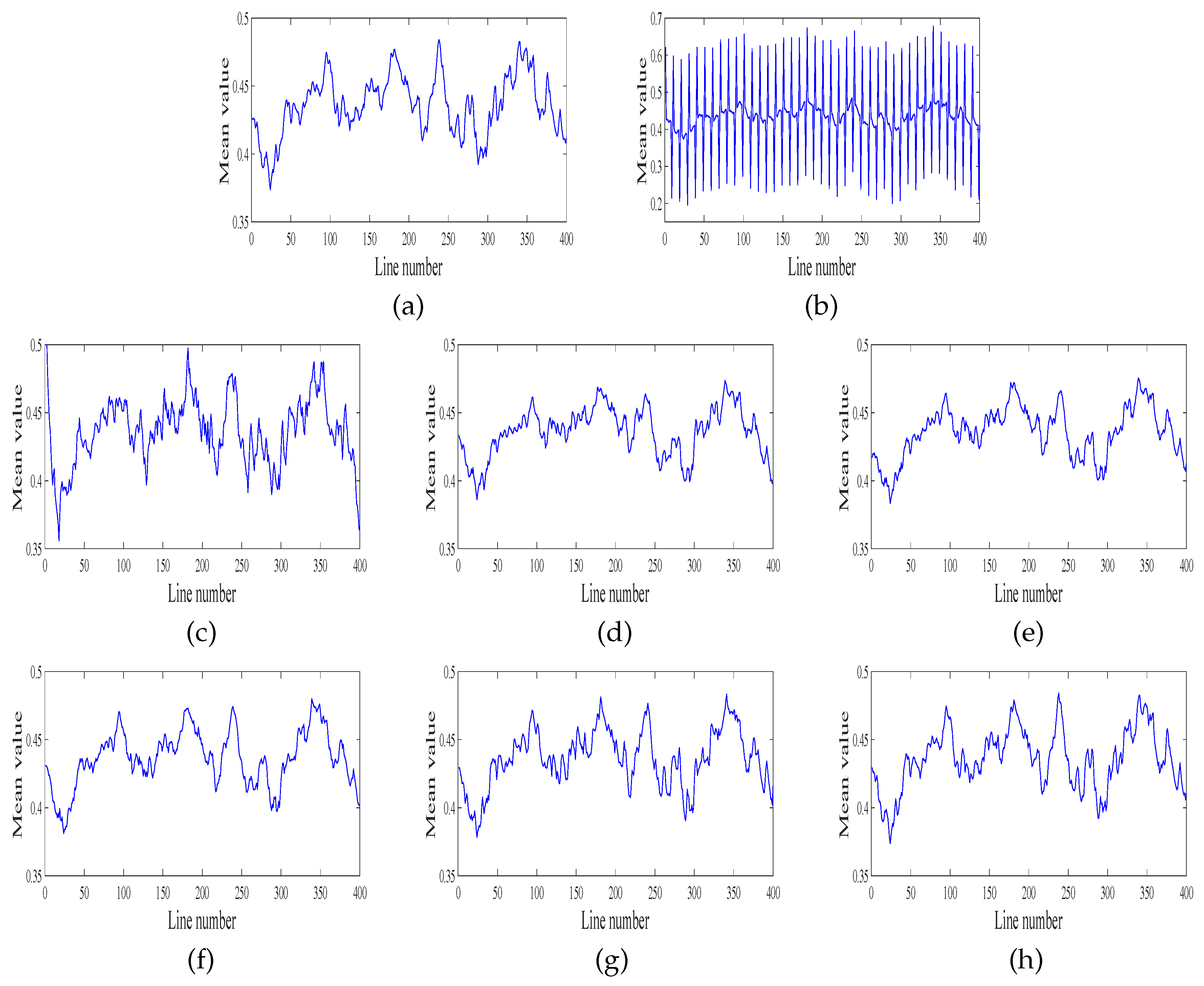
In simulated experiments, the mean cross-track profile of the first image of Figure 3 is shown in Figure 9. Note that Figure 9a shows the mean cross-track profile of the underlying image, and Figure 9b is the result of the degraded image. Moreover, Figure 9c–f shows the mean cross-track profile results of the six destriping methods, respectively. From the overall perspective, Figure 9d,e shows the obvious change of the intensity contrast. Seeing the details, Figure 9c–g has some mild fluctuations which are different from the underlying image in Figure 9a. The performance of the proposed method is almost same as that of the original one.

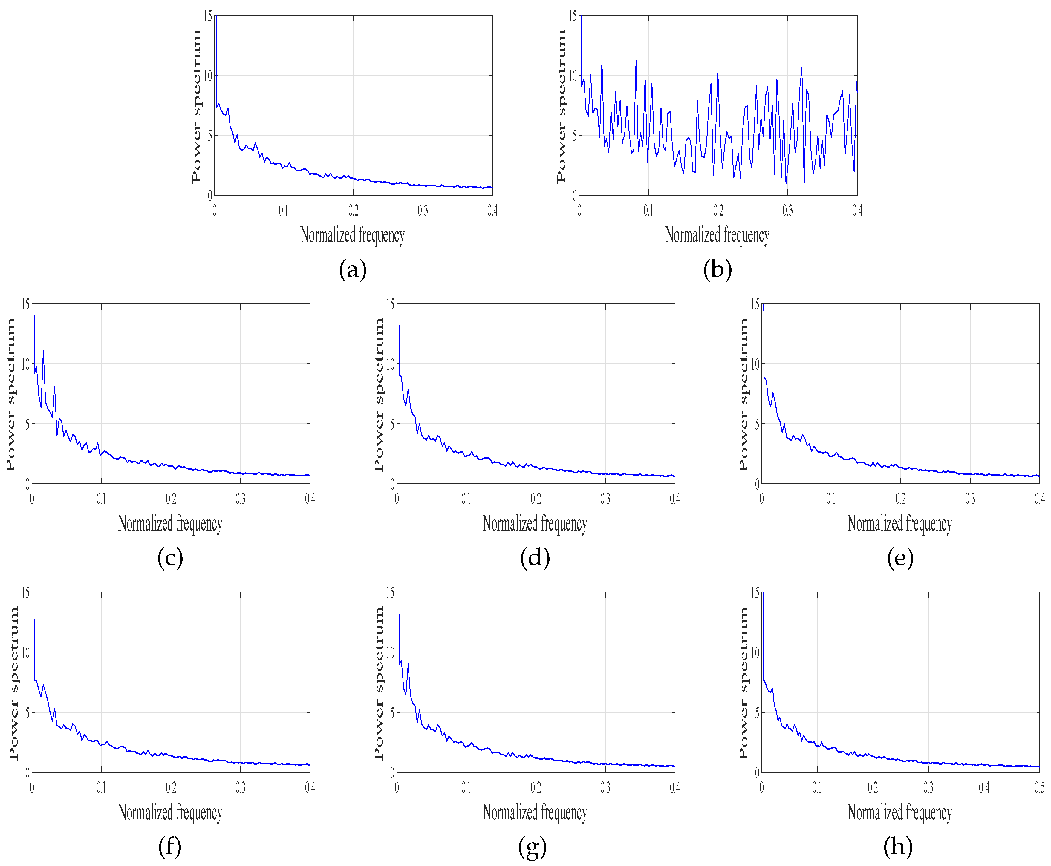
In addition, the power spectrum results of the second image of Figure 3 is shown in Figure 11. We denote the power spectrum results as Figure 11a–h which represent the power spectrum results of the underlying image, the degraded image and the destriping results of six methods, respectively. Figure 11c–g has more fluctuations which indicate these methods may have the stripe residuals or bring a little new noise in their destriping processes. Our method, i.e., Figure 11h, it not only removes all stripes, but also preserves almost the essential details such as edges.

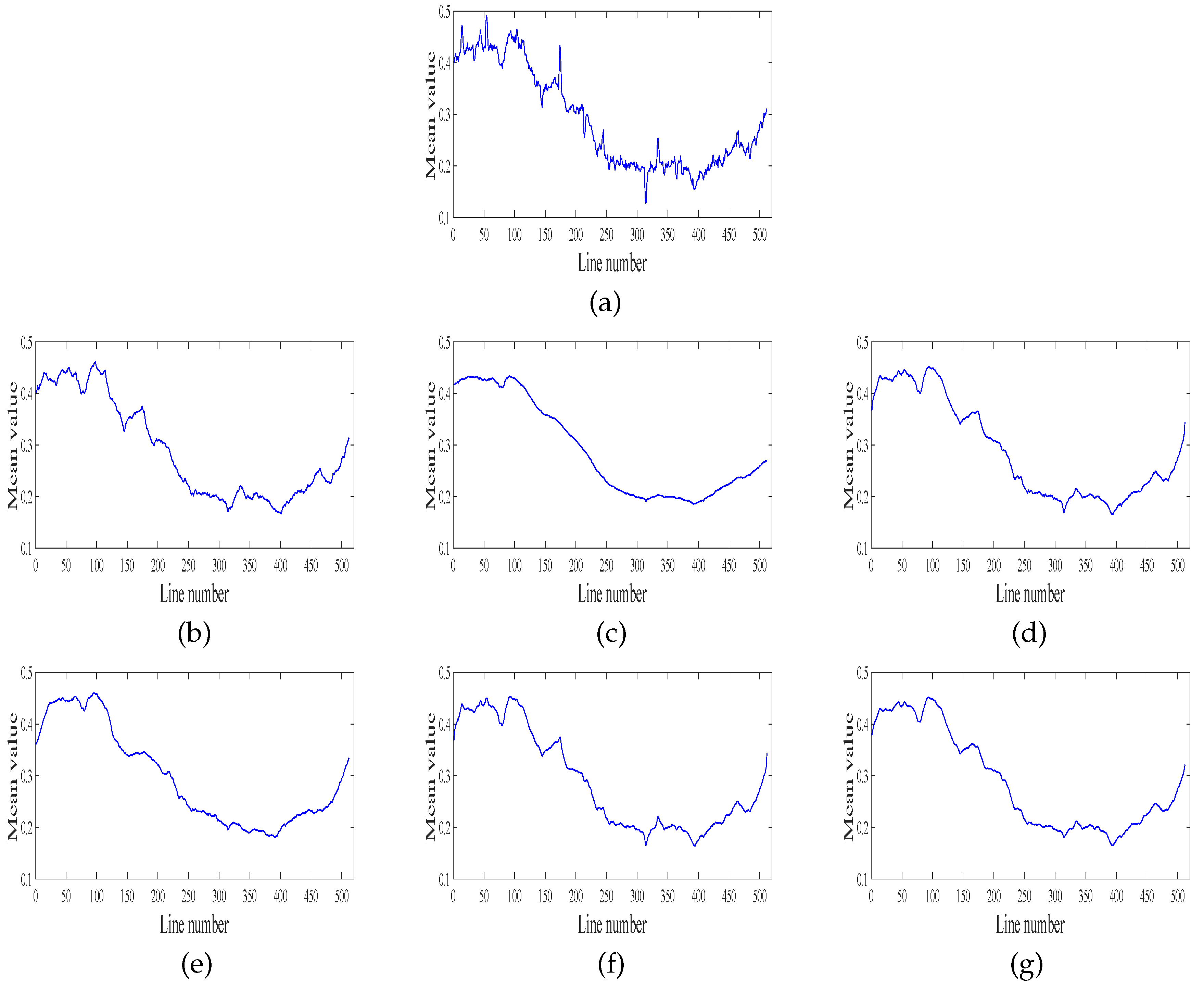
In real experiments, we also show the mean cross-track profile and the power spectrum in Figure 10 and Figure 12, respectively. Figure 10 shows the mean cross-track profile results of the first column of Figure 7. Note that Figure 10a is the mean cross-track profile result of the first real remote sensing image, and Figure 10b–g shows the profile results of the six destriping methods, respectively. In general, the profiles of the destriping method should smoothen huge fluctuates and maintain primary structure information. However, the profiles of WFAF and LRSID have obvious fluctuations where the stripes still exist, and that of SLD is over-smooth which loses a lot of underlying image details. In Figure 10d,e, although stripes are mostly removed, the destriping profiles have some mild blur and too much smoothness because of the unidirectional property of UTV and the global sparsity of GSLV, respectively. In addition, the profile of the proposed method, i.e., Figure 10g, can realize the desired result both on removing stripes and keeping underlying image details.

In Figure 12, the power spectrum results of the fourth example of Figure 7 are plotted. Figure 12a–h represent the power spectrum results of the fourth real remote sensing image and six destriping methods, respectively. We observe that the real remote sensing image in Figure 12a has many fluctuations where stand for stripes. According to the power spectrum results of the six methods in Figure 12b–f, although the stripes are almost removed well, there are still some slight blurring regions, while the proposed method shows the desired performance in Figure 12b.

4.3.2. The Influence of Different Regularization Terms in the Proposed Model

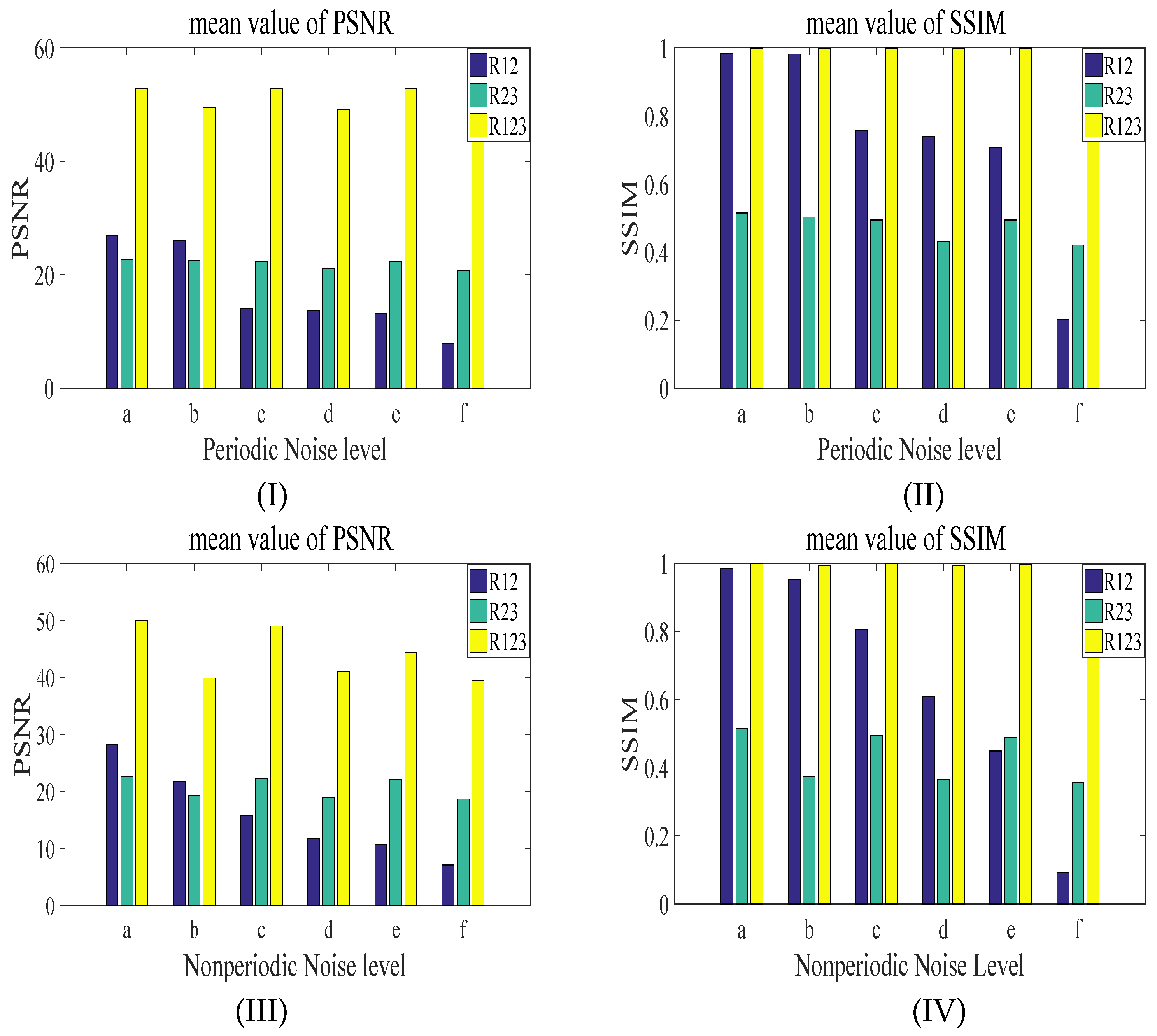
Fully considering the destriping problem in Equation (2) and the optimization model in Equation (13), we assume that ${\mathrm{R}}_2$ is a necessary term, since ${\mathrm{R}}_2$ is the only term to describe the property of the underlying image $\mathbf{u}$. To confirm whether both ${\mathrm{R}}_1$ and ${\mathrm{R}}_2$ are necessary priors as well as have important contribution to destriping performance, in Figure 13, we give the mean value of PSNR and SSIM for 32 images as before. Here, ${\mathrm{R}}_{12}$ represents ${\mathrm{R}}_1+{\mathrm{R}}_2$, ${\mathrm{R}}_{23}$ stands for ${\mathrm{R}}_2+{\mathrm{R}}_3$ and ${\mathrm{R}}_{123}$ represents ${\mathrm{R}}_1+{\mathrm{R}}_2+{\mathrm{R}}_3$ (i.e., the proposed model). Please find the definitions of ${\mathrm{R}}_1,{\mathrm{R}}_2,{\mathrm{R}}_3$ from Equations (10)–(12), respectively.

Figure 13I,II show the mean value of PSNR and the mean value of SSIM on 32 images same as before for periodic stripes. The periodic stripe levels in Figure 13a–f are (Per, 10, 0.2), (Per, 10, 0.6), (Per, 50, 0.2), (Per, 50, 0.6), (Per, 100, 0.2) and (Per, 100, 0.6), respectively. Moreover, Figure 13III,IV display the mean value of PSNR and the mean value of SSIM on 32 images for nonperiodic stripes. The nonperiodic stripe levels in Figure 13a–f stand for (NonPer, 10, 0.2), (NonPer, 10, 0.6), (NonPer, 50, 0.2), (NonPer, 50, 0.6), (NonPer, 100, 0.2) and (NonPer, 100, 0.6), respectively.

From the results in Figure 13, we can conclude three points. (1) The PSNR results of the proposed model (i.e., ${\mathrm{R}}_{123}$) have the best performance compared to those of the other two models (i.e., ${\mathrm{R}}_{12}$ and ${\mathrm{R}}_{13}$), and the SSIM results have the similar performance as compared with the PSNR results. (2) ${\mathrm{R}}_{23}$ shows more stability than ${\mathrm{R}}_{12}$ as the green bars do not significantly change with different stripes. (3) ${\mathrm{R}}_3$ actually plays a more important role than ${\mathrm{R}}_1$ with respect to PSNR (see Figure 13I,III. On the contrary, ${\mathrm{R}}_1$ plays a more important role than ${\mathrm{R}}_3$ with respect to SSIM (see Figure 13II,IV). Figure 13 demonstrates the effectiveness of the proposed model and the importance of the three terms.

5. Discussion

5.1. Parameter Value Selection

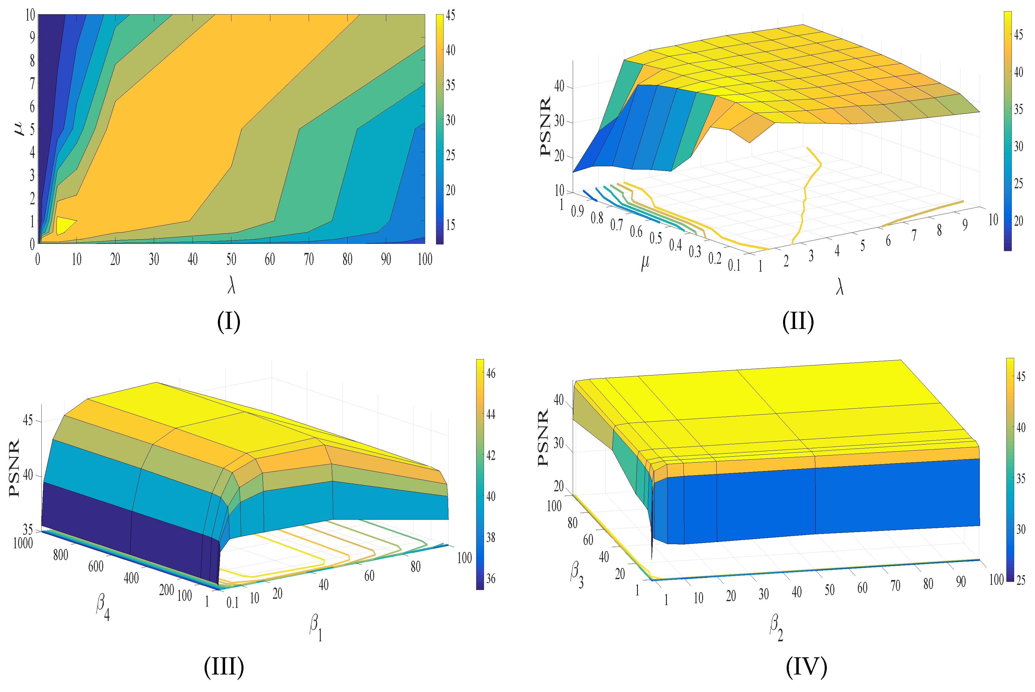
In this paper, the proposed method mainly involves six parameters $\lambda$, $\mu$, ${\beta }_1$, ${\beta }_2$, ${\beta }_3$, and ${\beta }_4$. The stripes of different types can be removed by setting different parameters. For example, if the stripes are dense, the $\mu$ should be small and the $\lambda$ should be large.

We tune the parameters by given strategy as follows. For instance, Figure 14, shows contour maps of PSNR values of different parameters setting for one example. In Figure 14I, we tune the regularization parameters $\lambda$, $\mu$, and fix ${\beta }_1$, ${\beta }_2$, ${\beta }_3$ and ${\beta }_4$. The yellow region is the best choice for the highest PSNR, and the orange is the next. Thus, we empirically set the regularization parameters within the range [0.1, 10] for $\lambda$ and [0.1, 1] for $\mu$ from this kind of contour maps for different examples. Similarly, from the Figure 14II, we empirically set the regularization parameters within the range [1, 10] for ${\beta }_2$ and ${\beta }_3$ since most of all PSNR results are similar. Then, ${\lambda }_1$ is empirically set with [1, 10²], and ${\beta }_4$ is set with [1, 10³]. Note that, we tune these parameters by 10 times interval in each parameter range. For instance, when tune ${\beta }_4$, we choose ${\beta }_4=1,10,100,1000$. Note that, the parameters cannot be automatically or adaptively chosen for different images. In this paper, we can have a good performance in the most of the situations. For most of the simulated experiments, we set the parameters with $\lambda =1$, $\mu =0.1$, ${\beta }_1=100,{\beta }_2={\beta }_3=10$, ${\beta }_4=1000$. For the real experiments, most of the examples show the superior results with $\lambda =10$, $\mu =1$ and ${\beta }_1={\beta }_2={\beta }_3={\beta }_4=1$. Note that, if fine tuning parameters based on this strategy for each image would get better results. However, we unify parameters to simplify the process of the parameter setting.

5.2. Limitation

In

Table 5. The computational cost of the methods.

	Image Size	WFAF	SLD	UTV	GSLV	LRSID	Ours
	300 × 300	0.2274	0.0466	0.2745	1.1442	4.2581	6.6541
	400 × 400	0.2603	0.0650	0.5711	1.7004	8.5212	15.2448

, we have shown the computed cost of two experiments. Actually, since the proposed method iteratively solves the ${\ell }_0$ norm as sub-problems by the designed algorithm, the proposed method indeed increases the computational burden compared with others methods. In particular, some statistic-based methods have a very fast speed. For example, SLD method only takes 0.046 s (for the image size 300 × 300). Actually, it is not easy to achieve the trade-off between the fast speed and the high accuracy. The more time cost may be viewed as a limitation of the proposed method.

6. Conclusions

In this paper, we proposed a directionally non-convex ${\ell }_0$ sparse model for remote sensing image destriping. We consider the directional and sparse characteristics of the stripe and the underlying image from local and global aspects. The non-convex ${\ell }_0$ norm can be effectively solved iteratively rather than hard threshold. This model was efficiently solved by the designed PADMM algorithm based on the MPEC reformulation. Furthermore, we also theoretically gave the corresponding proof of the convergence to the KKT point by this work. Experimental results on simulated and real data demonstrated the effectiveness of the proposed method, both quantitatively and visually. In particular, the proposed method obtained promising quantitative results, e.g., PSNR and SSIM, than some recent competitive methods on the average performance of 32 collected images. The power spectrum and spatial mean cross-track profiles were also employed to illustrate the superiority of the given method. Besides, for the real images, we also employed some non-reference indexes such as MICV and MMRD to compare the performance of different compared methods, which also demonstrated the effectiveness of our method.

In the future, we will try to speed up the proposed method using C language or parallel computing, and release the corresponding source code. In addition, we will extend the proposed model to the oblique stripes removal by fully considering the latent properties of oblique stripes. Furthermore, the proposed method was only applied to single-band image stripe removal. We may extend our framework to multispectral or hyperspectral image stripe removal by some intrinsic properties, e.g., low-rank and non-local priors.

References

- Chen, J.S.; Shao, Y.; Guo, H.D.; Wang, W.M.; Zhu, B.Q. Destriping CMODIS data by power filtering. IEEE Trans. Geosci. Remote Sens. 2003, 41, 2119–2124. [Google Scholar] [CrossRef]
- Münch, B.; Trtik, P.; Marone, F.; Stampanoni, M. Stripe and ring artifact removal with combined wavelet Fourier filtering. Opt. Express 2009, 17, 8567–8591. [Google Scholar]
- Pande-Chhetri, R.; Abd-Elrahman, A. De-striping hyperspectral imagery using wavelet transform and adaptive frequency domain filtering. ISPRS J. Photogramm. Remote Sens. 2011, 66, 620–636. [Google Scholar] [CrossRef]
- Pal, M.K.; Porwal, A. Destriping of Hyperion images using low-pass-filter and local-brightness-normalization. ISPRS J. Photogramm. Remote Sens. 2011, 66, 620–636. [Google Scholar]
- Gadallah, F.L.; Csillag, F.; Smith, E.J.M. Destriping multisensor imagery with moment matching. Int. J. Remote Sens. 2000, 21, 2505–2511. [Google Scholar] [CrossRef]
- Horn, B.K.P.; Woodham, R.J. Destriping Landsat MSS images by histogram modification. Comput. Graph. Image Process. 1979, 10, 69–83. [Google Scholar] [CrossRef]
- Weinreb, M.P.; Xie, R.; Lienesch, J.H.; Crosby, D.S. Destriping GOES images by matching empirical distribution functions. Remote Sens. Environ. 1989, 29, 185–195. [Google Scholar] [CrossRef]
- Wegener, M. Destriping multiple sensor imagery by improved histogram matching. Int. J. Remote Sens. 1990, 11, 859–875. [Google Scholar] [CrossRef]
- Rakwatin, P.; Takeuchi, W.; Yasuoka, Y. Restoration of Aqua MODIS band 6 using histogram matching and local least squares fitting. IEEE Trans. Geosci. Remote Sens. 2009, 47, 613–627. [Google Scholar] [CrossRef]
- Sun, L.X.; Neville, R.; Staenz, K.; White, H.P. Automatic destriping of Hyperion imagery based on spectral moment matching. Can. J. Remote Sens. 2008, 34, S68–S81. [Google Scholar] [CrossRef]
- Shen, H.F.; Jiang, W.; Zhang, H.Y.; Zhang, L.P. A piece-wise approach to removing the nonlinear and irregular stripes in MODIS data. Int. J. Remote Sens. 2014, 35, 44–53. [Google Scholar] [CrossRef]
- Fehrenbach, J.; Weiss, P.; Lorenzo, C. Variational algorithms to remove stationary noise: applications to microscopy imaging. IEEE Trans. Image Process. 2012, 21, 4420–4430. [Google Scholar] [CrossRef] [PubMed] [Green Version]
- Fehrenbach, J.; Weiss, P. Processing stationary noise: model and parameter selection in variational methods. SIAM J. Imaging Sci. 2014, 7, 613–640. [Google Scholar] [CrossRef]
- Escande, P.; Weiss, P.; Zhang, W.X. A variational model for multiplicative structured noise removal. J. Math. Imaging Vis. 2017, 57, 43–55. [Google Scholar] [CrossRef]
- Shen, H.F.; Zhang, L.P. A MAP-based algorithm for destriping and inpainting of remotely sensed images. IEEE Trans. Geosci. Remote Sens. 2009, 47, 1492–1502. [Google Scholar] [CrossRef]
- Chen, Y.; Huang, T.Z.; Zhao, X.L.; Deng, L.J.; Huang, J. Stripe noise removal of remote sensing images by total variation regularization and group sparsity constraint. Remote Sens. 2017, 9, 559. [Google Scholar] [CrossRef]
- Bouali, M.; Ladjal, S. Toward optimal destriping of MODIS data using a unidirectional variational model. IEEE Trans. Geosci. Remote Sens. 2011, 49, 2924–2935. [Google Scholar] [CrossRef]
- Zhang, H.Y.; He, W.; Zhang, L.P.; Shen, H.F.; Yuan, Q.Q. Hyperspectral image restoration using low-rank matrix recovery. IEEE Trans. Geosci. Remote Sens. 2014, 52, 4729–4743. [Google Scholar] [CrossRef]
- Zhou, G.; Fang, H.Z.; Yan, L.X.; Zhang, T.X.; Hu, J. Removal of stripe noise with spatially adaptive unidirectional total variation. Opt. Int. J. Light Electron Opt. 2014, 125, 2756–2762. [Google Scholar] [CrossRef]
- Liu, H.; Zhang, Z.L.; Liu, S.Y.; Liu, T.T.; Chang, Y. Destriping algorithm with L0 sparsity prior for remote sensing images. In Proceedings of the IEEE International Conference on Image Processing (ICIP), Quebec City, QC, Canada, 27–30 September 2015; pp. 2295–2299. [Google Scholar]
- Chang, Y.; Yan, L.X.; Fang, H.Z.; Liu, H. Simultaneous destriping and denoising for remote sensing images with unidirectional total variation and sparse representation. IEEE Geosci. Remote Sens. Lett. 2014, 11, 1051–1055. [Google Scholar] [CrossRef]
- Chang, Y.; Yan, L.X.; Fang, H.Z.; Luo, C.N. Anisotropic Spectral-Spatial Total Variation Model for Multispectral Remote Sensing Image Destriping. IEEE Trans. Image Process. 2015, 24, 1852–1866. [Google Scholar] [CrossRef] [PubMed]
- He, W.; Zhang, H.Y.; Zhang, L.P.; Shen, H.F. Total-variation-regularized low-rank matrix factorization for hyperspectral image restoration. IEEE Trans. Geosci. Remote Sens. 2016, 54, 178–188. [Google Scholar] [CrossRef]
- Zorzi, M.; Chiuso, A. Sparse plus low rank network identification: A nonparametric approach. Automatica 2017, 76, 355–366. [Google Scholar] [CrossRef]
- Zorzi, M.; Sepulchre, R. AR identification of latent-variable graphical models. IEEE Trans. Autom. Control 2016, 61, 2327–2340. [Google Scholar] [CrossRef]
- Liu, X.X.; Lu, X.L.; Shen, H.F.; Yuan, Q.Q.; Jiao, Y.L.; Zhang, L.P. Stripe Noise Separation and Removal in Remote Sensing Images by Consideration of the Global Sparsity and Local Variational Properties. IEEE Trans. Geosci. Remote Sens. 2016, 54, 3049–3060. [Google Scholar] [CrossRef]
- Chang, Y.; Yan, L.; Wu, T.; Zhong, S. Remote Sensing Image Stripe Noise Removal: From Image Decomposition Perspective. IEEE Trans. Geosci. Remote Sens. 2016, 54, 7018–7031. [Google Scholar] [CrossRef]
- Liu, J.; Huang, T.Z.; Selesnick, I.W.; Lv, X.G.; Chen, P.Y. Image restoration using total variation with overlapping group sparsity, Information Sciences. Inf. Sci. 2015, 295, 232–246. [Google Scholar] [CrossRef]
- Mei, J.J.; Dong, Y.Q.; Huang, T.Z.; Yin, W.T. Cauchy noise removal by nonconvex ADMM with convergence guarantees. J. Sci. Comput. 2018, 74, 743–766. [Google Scholar] [CrossRef]
- Ji, T.Y.; Huang, T.Z.; Zhao, X.L.; Ma, T.H.; Deng, L.J. A non-convex tensor rank approximation for tensor completion. Appl. Math. Model. 2017, 48, 410–422. [Google Scholar] [CrossRef]
- Carfantan, H.; Idier, J. Statistical linear destriping of satellite-based pushbroom-type images. IEEE Trans. Geosci. Remote Sens. 2010, 48, 1860–1871. [Google Scholar] [CrossRef]
- Rudin, L.I.; Osher, S.; Fatemi, E. Nonlinear total variation based noise removal algorithms. Phys. D Nonlinear Phenom. 1992, 60, 259–268. [Google Scholar] [CrossRef]
- Zhao, X.L.; Wang, F.; Huang, T.Z.; Ng, M.K.; Plemmons, R.J. Deblurring and sparse unmixing for hyperspectral images. IEEE Trans. Geosci. Remote Sens. 2013, 51, 4045–4058. [Google Scholar] [CrossRef]
- Ma, T.H.; Huang, T.Z.; Zhao, X.L.; Lou, Y.F. Image Deblurring With an Inaccurate Blur Kernel Using a Group-Based Low-Rank Image Prior. Inf. Sci. 2017, 408, 213–233. [Google Scholar] [CrossRef]
- Getreuer, P. Total variation inpainting using split Bregman. Image Process. Line 2012, 2, 147–157. [Google Scholar] [CrossRef]
- Yuan, G.Z.; Ghanem, B. l0TV: A new method for image restoration in the presence of impulse noise. In Proceedings of the IEEE Conference on Computer Vision and Pattern Recognition, Boston, MA, USA, 7–12 June 2015; pp. 5369–5377. [Google Scholar]
- Shen, H.F.; Li, X.H.; Cheng, Q.; Zeng, C.; Yang, G.; Li, H.F. Missing information reconstruction of remote sensing data: A technical review. IEEE Geosci. Remote Sens. Mag. 2015, 3, 61–85. [Google Scholar] [CrossRef]
- Dong, B.; Zhang, Y. An efficient algorithm for ℓ0 minimization in wavelet frame based image restoration. J. Sci. Comput. 2013, 54, 350–368. [Google Scholar] [CrossRef]
- Fan, Y.R.; Huang, T.Z.; Ma, T.H.; Zhao, X.L. Cartoon-texture image decomposition via non-convex low-rank texture regularization. J. Frankl. Inst. 2017, 354, 3170–3187. [Google Scholar] [CrossRef]
- Lu, Z.S.; Zhang, Y. Sparse approximation via penalty decomposition methods. SIAM J. Optim. 2013, 23, 2448–2478. [Google Scholar] [CrossRef]
- Donoho, D.L. De-noising by soft-thresholding. IEEE Trans. Inf. Theory 1995, 41, 613–627. [Google Scholar] [CrossRef]
- Wang, Z.; Bovik, A.C.; Sheikh, H.R.; Simoncelli, E.P. Image Quality Assesment: From Error Visibility to Structural Similarity. IEEE Trans. Image Process. 2004, 13, 600–612. [Google Scholar] [CrossRef] [PubMed]
- He, B.S.; Yuan, X.M. On the O(1/n) Convergence Rate of the Douglas Rachford Alternating Direction Method. SIAM J. Numer. Anal. 2012, 50, 700–709. [Google Scholar] [CrossRef]
- Deng, W.; Yin, W.T. On the global and linear convergence of the generalized alternating direction method of multipliers. J. Sci. Comput. 2016, 663, 889–916. [Google Scholar] [CrossRef]
- Wen, Z.W.; Yang, C.; Liu, X.; Marchesini, S. Alternating direction methods for classical and ptychographic phase retrieval. Inverse Probl. 2012, 28, 115010. [Google Scholar] [CrossRef]
- Fazel, M.; Pong, T.K.; Sun, D.F.; Tseng, P. Hankel matrix rank minimization with applications to system identification and realization. SIAM J. Matrix Anal. Appl. 2013, 34, 946–977. [Google Scholar] [CrossRef]
Figure 1.
Framework of the proposed destriping method.
Figure 2.
The number of nonzero elements of (a) and (b), where is estimated from a real image example (see Figure 3) by the method [26]. The y-axis represents the number of nonzero elements of and , respectively, and the x-axis stands for the image pixel value whose range is [0, 1].
Figure 3.
The visual results of different simulated images. From top to bottom: underlying images, degraded images, the destriping results of WFAF, SLD, UTV, GSLV, LRSID, and Ours. The degraded images in the second row are, respectively, added the stripes (from left to right): (Per, 10, 0.2), (NonPer, 100, 0.4), (NonPer, 50, 0.2), (NonPer, 60, 0.4), (NonPer, 100, 0.4) and (NonPer, 50, 0.6). Readers are recommended to zoom in all figures for better visibility.
Figure 4.
The zoom results of different simulated images in Figure 3. From top to bottom: zoom of the underlying images, the degraded images, the destriping results of WFAF, SLD, UTV, GSLV, LRSID, and Ours. Note that the levels of stripes are same as Figure 3.
Figure 5.
The stripes of different simulated images in Figure 3. From top to bottom: the added stripes on the underlying image, the extracted stripe components of WFAF, SLD, UTV, GSLV, LRSID, and Ours. Note that the levels of stripes are same as Figure 3.
Figure 6.
The PSNR and SSIM performance on 32 images for the stripes (Per, 100, 0.6) and (NonPer, 50, 0.2). The x-axis represents each image and the quantitative results are shown in the y-axis. (I) and (II) are the PSNR and SSIM results for the stripes (Per, 100, 0.6), respectively. (III) and (IV), respectively, represent the PSNR and SSIM performance of the stripes (NonPer, 50, 0.2).
Figure 7.
The visual results of different real images. From top to bottom: the real images, the destriping results of WFAF, SLD, UTV, GSLV, LRSID, and Ours. Readers are recommended to zoom in all figures for better visibility.
Figure 8.
The stripes of different real images in Figure 7. From top to bottom: the extracted stripe components of WFAF, SLD, UTV, GSLV, LRSID, and Ours.
Figure 9.
Spatial mean cross-track profiles for simulated image of the first simulated example of Figure 3: (a) underlying image; (b) degraded image; and destriping results by: (c) WFAF; (d) SLD; (e) UTV; (f) GSLV; (g) LRSID; and (h) Ours.
Figure 10.
Spatial mean cross-track profiles for the first real example of Figure 7: (a) real image; and destriping results by: (b) WFAF; (c) SLD; (d) UTV; (e) GSLV; (f) LRSID; and (g) Ours.
Figure 11.
Power spectrum for simulated image of the second example of Figure 7: (a) underlying image; (b) degraded image; and destriping results by: (c) WFAF; (d) SLD; (e) UTV; (f) GSLV; (g) LRSID; and (h) Ours.
Figure 12.
Power spectral for the forth real example of Figure 7: (a) real image; and destriping results by: (b) WFAF; (c) SLD; (d) UTV; (e) GSLV; (f) LRSID; and (g) Ours.
Figure 13.
The influence of different terms in the proposed model. represents , stands for and represents (i.e., the proposed model). (I) The mean PSNR performance on 32 images for periodic stripes with different stripe levels; (II) The mean SSIM performance on 32 images for periodic stripes with different stripe levels; The stripe levels (a–f) stand for (Per, 10, 0.2), (Per, 10, 0.6), (Per, 50, 0.2), (Per, 50, 0.6), (Per, 100, 0.2) and (Per, 100, 0.6), respectively. (III) The mean PSNR performance on 32 images for nonperiodic stripes with different stripe levels; (IV) The mean SSIM performance on 32 images for nonperiodic stripes with different stripe levels. The stripe levels (a–f) stand for (NonPer, 10, 0.2), (NonPer, 10, 0.6), (NonPer, 50, 0.2), (NonPer, 50, 0.6), (NonPer, 100, 0.2) and (NonPer, 100, 0.6), respectively.
Figure 14.
Parameters value selection