Automatic Building Segmentation of Aerial Imagery Using Multi-Constraint Fully Convolutional Networks

Abstract

Automatic building segmentation from aerial imagery is an important and challenging task because of the variety of backgrounds, building textures and imaging conditions. Currently, research using variant types of fully convolutional networks (FCNs) has largely improved the performance of this task. However, pursuing more accurate segmentation results is still critical for further applications such as automatic mapping. In this study, a multi-constraint fully convolutional network (MC–FCN) model is proposed to perform end-to-end building segmentation. Our MC–FCN model consists of a bottom-up/top-down fully convolutional architecture and multi-constraints that are computed between the binary cross entropy of prediction and the corresponding ground truth. Since more constraints are applied to optimize the parameters of the intermediate layers, the multi-scale feature representation of the model is further enhanced, and hence higher performance can be achieved. The experiments on a very-high-resolution aerial image dataset covering 18 km${}^2$ and more than 17,000 buildings indicate that our method performs well in the building segmentation task. The proposed MC–FCN method significantly outperforms the classic FCN method and the adaptive boosting method using features extracted by the histogram of oriented gradients. Compared with the state-of-the-art U–Net model, MC–FCN gains 3.2% (0.833 vs. 0.807) and 2.2% (0.893 vs. 0.874) relative improvements of Jaccard index and kappa coefficient with the cost of only 1.8% increment of the model-training time. In addition, the sensitivity analysis demonstrates that constraints at different positions have inconsistent impact on the performance of the MC–FCN.

1. Introduction

Due to the frequent changing of landmarks, especially for rapidly developing cities, it is essential to be able to immediately update such changes for the purposes of navigation and urban planning. Remote-sensing technologies, such as satellite and aerial photography, can capture images of certain areas routinely and serve as useful tools for these types of tasks. In recent years, due to the technical development of imaging sensors and emerging platforms, such as unmanned aerial vehicles, the availability and accessibility of high-resolution remote-sensing imagery have increased dramatically [1]. Meanwhile, the state-of-the-art deep-learning methods have largely improved the performance of image segmentation. However, more accurate building segmentation results are still critical for further applications such as automatic mapping.

Building detection can be viewed as a specific image segmentation application that segments buildings from their surrounding background. Over the past decades, a great amount of image segmentation algorithms have been proposed. The majority of these algorithms can be classified into four categories: threshold-based, edge-based, region-based and classification-based methods. Image thresholding is a simple and commonly used segmentation method. Pixels with different values are allocated to different parts according to manually or automatically selected thresholds [2]. Normally, image thresholding is not capable of differentiating among different regions with similar grayscale values. Edge-based methods adopt edge-detection filters, such as Laplacian of Gaussian [3], Sobel [4] and Canny [5], to detect the abrupt changes among neighboring pixels and generate boundaries for segmentation. Region-based methods segment different parts of an image through clustering [6,7,8,9], region-growing [10] or shape analysis [11,12]. Due to the variety of illuminance and texture conditions of an image, edge-based or region-based methods cannot provide stable and generalized results. Unlike the other three methods, classification-based methods treat image segmentation as a process of classifying the category of every pixel [13]. Since the segmentation is made by classifying every pixel, the classification-based method can produce more precise segmentations with proper feature extractors and classifiers.

Before deep learning, traditional classification-based methods must undergo a two-step procedure of feature extraction and classification. The spatial and textural features of an image are extracted through mathematical feature descriptors, such as haar-like [14], scale-invariant feature transform [15], local binary pattern [16], and histogram of oriented gradients (HOG) [17]. After that, the prediction for every pixel is made on the basis of the extracted features through classifiers such as support vector machines [18], adaptive boosting (AdaBoost) [19], random forests [20] and conditional random fields (CRF) [21]. However, because of the complexity of building structures and also because of strong similarities with other classes (e.g., pieces of roads), the prediction results rely heavily on manual feature design and adaptation, which easily leads to bias and poor generalization.

With the development of algorithms, computational capability and the availability of big data, convolutional neural networks (CNNs) [22] have attracted more and more attention in this field. Unlike two-step methods requiring artificial feature extraction, CNNs can automatically extract features and make classifications through sequential convolutional and fully connected layers. The CNN method can be considered as a one-step method that combines feature extraction and classification within a single model. Since the feature extraction is learned from the data itself, CNN usually possesses better generalization capability.

In the early stages, patch-based CNN approaches label a pixel by classifying the patch that centers around that pixel [23,24]. Even for a small patch of 32 × 32 pixels, to cover the whole area, the memory cost of these patch-based methods increases by 32 × 32 times. For larger areas or patch sizes, these approaches encounter dramatically increased memory cost and significantly reduced processing efficiency [25]. Fully convolutional networks (FCNs) improve this problem greatly by replacing the fully connected layer with upsampling operations [26]. Through multiple convolutional and upsampling operations, the FCN model allows efficient pixel-to-pixel classification of an image. However, the FCN model and other similar convolutional encoder–decoder models, such as SegNet [27] and DeconvNet [28], use only part of layers to generate the final output, leading to lower edge accuracy.

To overcome this limitation, one of the state-of-the-art fully convolutional models, U–Net [29], adopts bottom-up/top-down architecture with skip connections that combine both the lower and higher layers to generate the final output, resulting in better performance. However, the U–Net model also has its own limitations: (1) At training phase, the parameter updating of both-end layers is prior to those of the intermediate layers (i.e., the layers closer to the top of the feature pyramid) during every backpropagation iteration, which makes the intermediate layers less semantically meaningful [30]; and (2) the existing study has indicated that multi-scale feature representation (contributed by both end layers and intermediate layers) is very useful for improving the performance and generalization capability of the model [31], while in the classic U–Net model, due to the loose constraint for the intermediate features, the multi-scale feature representation could be further enhanced if explicit constraints are applied directly on these layers.

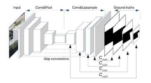
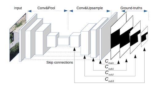
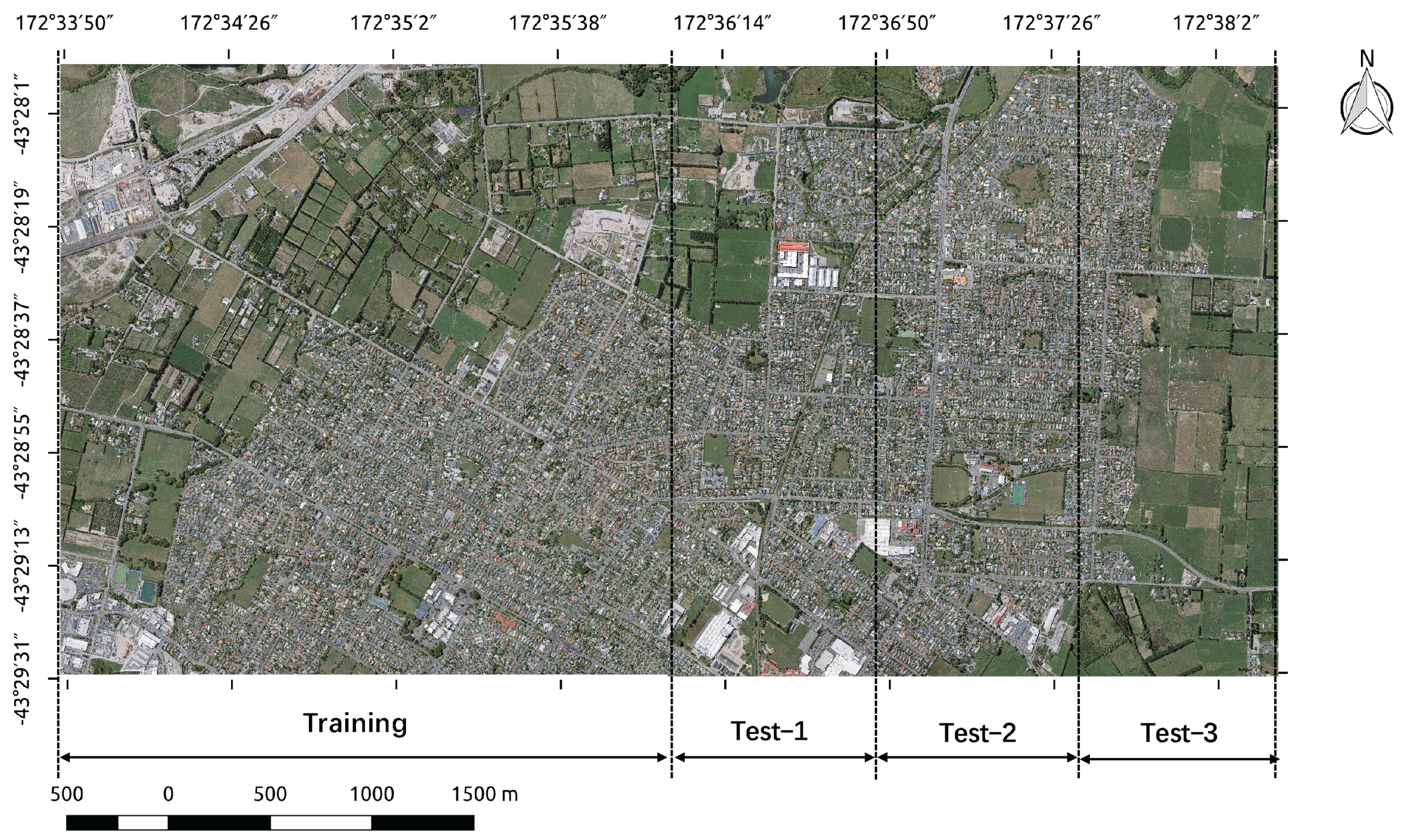
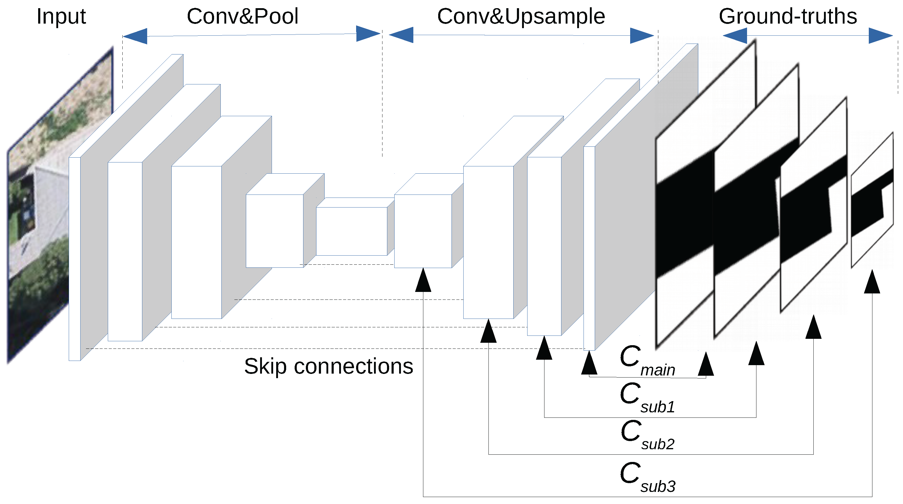
Based on the above analysis, we propose a novel architecture of deep fully convolutional networks with multi-constraints, termed multi-constraint fully convolutional networks (MC–FCNs). The MC–FCN model adopts the basic structure of a U–Net and adds multi-scale constraints for variant layers. Here, an optimization target between the prediction and the corresponding ground truth for a certain layer is defined as a constraint. During every iteration, parameters are updated through the multi-constraints, which prevents the parameters from biasing to a single constraint. Also, the constraints are applied on different layers, which helps to better optimize the hidden representation of variant layers. The experiments on a very-high-resolution aerial image dataset with a coverage area of 18 km${}^2$ in New Zealand demonstrate the effectiveness of the proposed MC–FCN model. In comparative trials, the mean values of Jaccard index, overall accuracy and kappa coefficient achieved by our method are 0.833, 0.976 and 0.893, respectively, which are better than those achieved by the classic U–Net model, and significantly outperform the classic FCN and the Adaboost methods using features extracted by HOG. Furthermore, the sensitivity analysis indicates that constraints applied on different layers have impacts of varying degrees on the improvement performance of the proposed model. The main contributions of this study are summarized as follows: (1) We propose a novel multi-constraint fully convolutional architecture that increases the performance of the state-of-the-art method (i.e., U–Net) in building segmentation of very-high-resolution aerial imagery; and (2) we further analyze the effects of different combinations of constraints in MC–FCN to explore how these constraints affect the performance of the deep CNN models.

The remainder of this paper is organized as follows. The materials and methods are described in Section 2, where the configuration details of the network are also presented. In Section 3, the results of evaluation and the sensitivity analysis are introduced. The discussion and conclusions are made in Section 4 and Section 5, respectively.

2. Materials and Methods

2.1. Data

The performance of the deep-learning model heavily relies on large-scale learning samples. In this paper, aerial images with coverage areas of 18 km${}^2$ in New Zealand are used as the experimental data (see Figure 1).

The aerial image dataset and the corresponding building outlines (stored as polygon shapefiles) were downloaded from the website of Land Information of New Zealand (https://data.linz.govt.nz/layer/53413-nz-building-outlines-pilot/). The aerial images were captured during the flying seasons of 2015 and 2016. The provider converted the original images into orthophotos with a spatial resolution of 0.075 m and divided them into tiles. The tiles within the study areas were merged into a single mosaic for the experiment. Meanwhile, some of the building outlines were extracted by aligning with their ground positions rather than their roofs. Considering that our target was to precisely detect the buildings’ roofs, before the experiment, the whole dataset was carefully scanned and each polygon manually adjusted to align strictly with the corresponding roofs. As shown in Figure 1, the study area was divided into training and testing areas of equal size including 8258 and 9134 building objects, respectively. The training area consists of almost evenly distributed non-housing background and residential areas. To evaluate the model’s ability of building detection under variant land-cover conditions, the test area was further divided into three subregions: Test-1, Test-2 and Test-3. The Test-1 region occupies large residential areas, but also includes quite a lot of farmland and lakes. The Test-2 area is dominated by residential areas and some traffic roads. In contrast, the Test-3 region has only a small portion of residential areas but a large area of background vegetation.

2.2. Method

Figure 2 shows the scheme of the study. The aerial imagery of the study area undergoes a framework of data preprocessing to generate training and testing data (see Section 2.2.1). Then, our proposed MC–FCN model is trained using 70% of the training data. The remaining 30% of the training data is used for cross-validation. The trained model with proper hyperparameters will be chosen to make predictions on the testing data and evaluated by five commonly used evaluation metrics including precision, recall, Jaccard index or intersection over union (IoU) [32], overall accuracy [33] and kappa coefficient [34]. Smoothing the final segmentation maps using a CRF or simple morphological operations has previously proven to increase the performance of the classification results [35]. However, to clearly reflect the classification capability of different methods, evaluation metrics are computed without any post-processing for the segmentation maps.

2.2.1. Data Preprocessing

The whole study area is evenly divided into two areas for training and testing. The testing area is further divided into three regions with various distributions. The aerial imagery of the training area and testing regions are processed by a sliding window of 224 × 224 pixels to generate data for model training, cross-validation and testing. Similarly, a consistent size of ground truth dataset is generated. Since our method consists of four constraints with variant sizes, bilinear interpolation is applied to generate three subsampled ground truths. For each subsampled ground truth, the pixels with low interpolated values are eliminated as non-pure samples using a simple threshold of 128 (the original gray value of ground truth is 255). To prevent the training data from biasing towards the background, thresholding is applied to eliminate image slices with low building-cover rates.

2.2.2. MC–FCN

The model of CNN was invented by Lecun et al. in 1998 [36]. The method incorporated two important concepts, sparse connectivity and shared weights, which greatly reduced the number of weights and improved efficiency. The basic structures of CNNs include a convolutional layer, nonlinear activation, a pooling layer and a fully-connected layer.

Figure 3 shows the architecture of the proposed multi-constraint fully convolutional network (MC–FCN). The network follows all the basic structures of CNNs but discards the fully connected layers. Several skip connections are applied between the symmetric layers in the bottom-up/top-down structure following the design of the U–Net. Although the classic U–Net model is already very powerful, it still can be improved on the following limitations:

• According to backpropagation algorithms, at every iteration, the closer to the output layer, the more significant will be the updating of the parameters; thus, during training, the model’s performance becomes more sensitive to the layer used to compute the final loss.
• Models that minimize only the difference between the final output and ground truth will lead to insufficient constraints for the middle layers, and applying more constraints on the intermediate layers can enhance the multi-scale feature representation by further optimizing the parameters in these layers.

Facing these problems, the proposed MC–FCN model introduces three extra multi-scale subconstraints, which are computed between different upsampled feature layers and their corresponding ground truths. In MC–FCN model, the parameters are updated through the multi-constraints, which prevents the parameters from biasing to a single constraint. Also, the constraints are applied in different layers, helping to simultaneously enhance the hidden representations of variant layers. As shown in Figure 3, the left part of the MC–FCN generates a bottom-up/top-down architecture through sequential convolutional and pooling (conv & pool), and convolutional and upsampling (conv & upsample), blocks with skip connections.

The convolution operation is an element-wise multiplication operation within a specific kernel [22]. The output of the convolution operation will be further handled by nonlinear activation function of the rectified linear unit (ReLU) [37]. The pooling layer is a subsampling operation for reducing the height and width. In this research, max-pooling [38] is adopted. To generate the final output with equal height and width, sequential bilinear upsampling [39] and skip-connection operations are performed. A skip connection is a concatenating operation between two related matrices with consistent heights and widths.

As the target of the output is a binary classification of building and non-building, the sigmoid function is chosen to generate the predictions for each layer:

$$\begin{array}{cc}\hfill z_{i,j}& =b+\sum _{k^{\prime }=1}^c{w}_{k^{\prime }}\times x_{i,j,k^{\prime }}\hfill \\ \hfill y_{i,j}& =\frac{1}{1+e^{-z_{i,j}}}.\hfill \end{array}$$

(1)

The w ∈ R${}^c$ and b ∈ R${}^1$ denote the weights and bias, respectively. The range of prediction $y_{i,j}$ is limited to [0, 1].

Instead of the simple mean squared error (MSE), binary cross entropy [40] is chosen to calculate the kth constraint (C${}_k$) between every prediction and relative ground truth for better convergence during training iterations. The formula is:

$$\begin{array}{cc}\hfill C_k& =-\frac{1}{h^k\times w^k}\sum _{i=1,j=1}^{h^k,w^k}{g}_{i,j}^k\times log(y_{i,j}^k)+(1-g_{i,j}^k)\times log(1-y_{i,j}^k),\hfill \end{array}$$

(2)

where $h^k$ and $w^k$ are the height and width of the kth prediction $y^k$ and ground truth $g^k$. The value of $g_{i,j}^k$ is 1 if the observation is in class 1; otherwise, the value is 0. The $y_{i,j}^k$ is the predicted probability of the pixel being in class 1.

To accelerate deep-network training and avoid bias, the batch normalization (BN) layer [41] is heavily applied after every convolutional layer.

Through sequential conv & upsample blocks and skip connections, the MC–FCN model generates pyramid-like feature layers. For every feature layer from the feature pyramid, a single kernel of a 1 × 1 convolution operation following by sigmoid activation is applied to generate prediction for that layer. Then, the constraint for each layer can be calculated by the binary cross entropy between each prediction and related ground truth. According to the distance from the final convolution layer, these constraints were denoted as C${}_{main}$, C${}_{sub1}$, C${}_{sub2}$ and C${}_{sub3}$. Thus, the final loss of the MC–FCN can be formulated as:

$$\begin{array}{cc}\hfill Loss& =\alpha \times C_{main}+\beta \times C_{sub1}+\gamma \times C_{sub2}+\delta \times C_{sub3},\hfill \end{array}$$

(3)

where the sum of $\alpha$, $\beta$, $\gamma$ and $\delta$ is set to 1.0. The best performance of the MC–FCN model was achieved using weights of $\alpha$ = 0.5, $\beta$ = 0, $\gamma$ = 0 and $\delta$ = 0.5.

With all of the above layers being trained by mini-batch stochastic gradient descent (SGD) and back propagation (BP) algorithms to minimize the final loss, the MC–FCN model learns how to map from the input RGB image to the equal-size binary segmentation map.

2.3. Experimental Setup

2.3.1. Architecture of the MC–FCN

The architecture of the MC–FCN consists of four sequential conv & pool and four conv & upsample blocks with skip connections between the second batch normalization (BN) layer of the conv & pool block and upsampling layer of conv & upsample blocks. The output of each block served as the input for the next block. The initial input of the MC–FCN was the RGB image with a size of 224 × 224 pixels.

As shown in

Table 1. Configuration of conv & pool block.

Layer	Output Shape	Kernel Size	Scale	Number of Kernels	Connect to
Conv_1	(h, w, k)	(3, 3)	-	k	Input
ReLU_1	(h, w, k)	-	-	-	Conv_1
BN_1	(h, w, k)	-	-	-	ReLU_1
Conv_2	(h, w, k)	(3, 3)	-	k	BN_1
ReLU_2	(h, w, k)	-	-	-	Conv_2
BN_2	(h, w, k)	-	-	-	ReLU_2
Maxpool_1	(h/2, w/2, k)	-	(2, 2)	-	BN_2

The h and w represent the height and width of input layer, respectively. * BN_2 layer concatenated with upsample layer of conv & upsample block.

, each conv & pool block has two convolutional layers, followed by two ReLU activations, two batch normalization layers and one max-pooling layer. The number of kernels of four conv & pool blocks are [24, 48, 96, 192].

As can be seen in

Table 2. Configuration of conv & upsample block.

Layer	Output Shape	Kernel Size	Scale	Number of Kernels	Connect to
Upsample_1’	$(2\times {\mathrm{h}}^{\prime },2\times {\mathrm{w}}^{\prime },\mathrm{d})$	-	(2, 2)	-	Input’
Skip_1’	$(2\times {\mathrm{h}}^{\prime },2\times {\mathrm{w}}^{\prime },\mathrm{d}+\mathrm{k})$	-	-	-	Upsample_1’ & BN_2
Conv_1’	$(2\times {\mathrm{h}}^{\prime },2\times {\mathrm{w}}^{\prime },{\mathrm{k}}^{\prime })$	(3, 3)	-	k’	Skip_1’
ReLU_1’	$(2\times {\mathrm{h}}^{\prime },2\times {\mathrm{w}}^{\prime },{\mathrm{k}}^{\prime })$	-	-	-	Conv_1’
BN_1’	$(2\times {\mathrm{h}}^{\prime },2\times {\mathrm{w}}^{\prime },{\mathrm{k}}^{\prime })$	-	-	-	ReLU_1’
Conv_2’	$(2\times {\mathrm{h}}^{\prime },2\times {\mathrm{w}}^{\prime },{\mathrm{k}}^{\prime })$	(3, 3)	-	k’	BN_1’
ReLU_2’	$(2\times {\mathrm{h}}^{\prime },2\times {\mathrm{w}}^{\prime },{\mathrm{k}}^{\prime })$	-	-	-	Conv_2’
BN_2’	$(2\times {\mathrm{h}}^{\prime },2\times {\mathrm{w}}^{\prime },{\mathrm{k}}^{\prime })$	-	-	-	ReLU_2’

The h’, w’ and d represent height, width and depth of input layer, respectively. * BN_2’ layer generates prediction.

, there is a single upsample and skip-connection layer, and double convolution, ReLU activation and batch normalization layers in each conv & upsample block. The number of kernels of four conv & upsample blocks are [192, 96, 48, 24]. A single 1 × 1 convolutional kernel followed by sigmoid activation is applied to every second batch-normalization layer of conv & upsample blocks to generate predictions. Then, the constraint is calculated through computing the binary cross entropy between the predictions and ground truths.

2.3.2. Various Combinations of Constraints

To further analyze the significance of the constraints on different scales, different numbers of constraints are used for comparison. The MC–FCN models using single $C_{main}$ or $C_{main}$ along with different numbers of $C_{sub}$ are trained and validated using the same training and testing data. The values of $\alpha$, $\beta$, $\gamma$ and $\delta$ of models with different numbers of constraints are listed in

Table 3. Weights in models with different numbers of constraints.

Number of Subconstraints	$\mathit{\alpha }$-Value	$\mathit{\beta }$-Value	$\mathit{\gamma }$-Value	$\mathit{\delta }$-Value
0	1/1	-	-	-
1	1/2	1/2	-	-
2	1/3	1/3	1/3	-
3	1/4	1/4	1/4	1/4

.

During neural network iteration, constraints from different layers contribute unequally to the sample parameter that might be different to the model performance. To investigate the relative importance of the three subconstraints ($C_{sub1-3}$), the experiment to compare the four MC–FCN models with various combinations of constraints was conducted. The model with the single main constraint served as the control. The weights used for each model are listed in

Table 4. Weights in models of various combinations of constraints.

Constraint Combination	$\mathit{\alpha }$-Value	$\mathit{\beta }$-Value	$\mathit{\gamma }$-Value	$\mathit{\delta }$-Value
$C_{main}$	1.0	-	-	-
$C_{main}+C_{sub1}$	0.5	0.5	-	-
$C_{main}+C_{sub2}$	0.5	-	0.5	-
$C_{main}+C_{sub3}$	0.5	-	-	0.5

.

3. Results

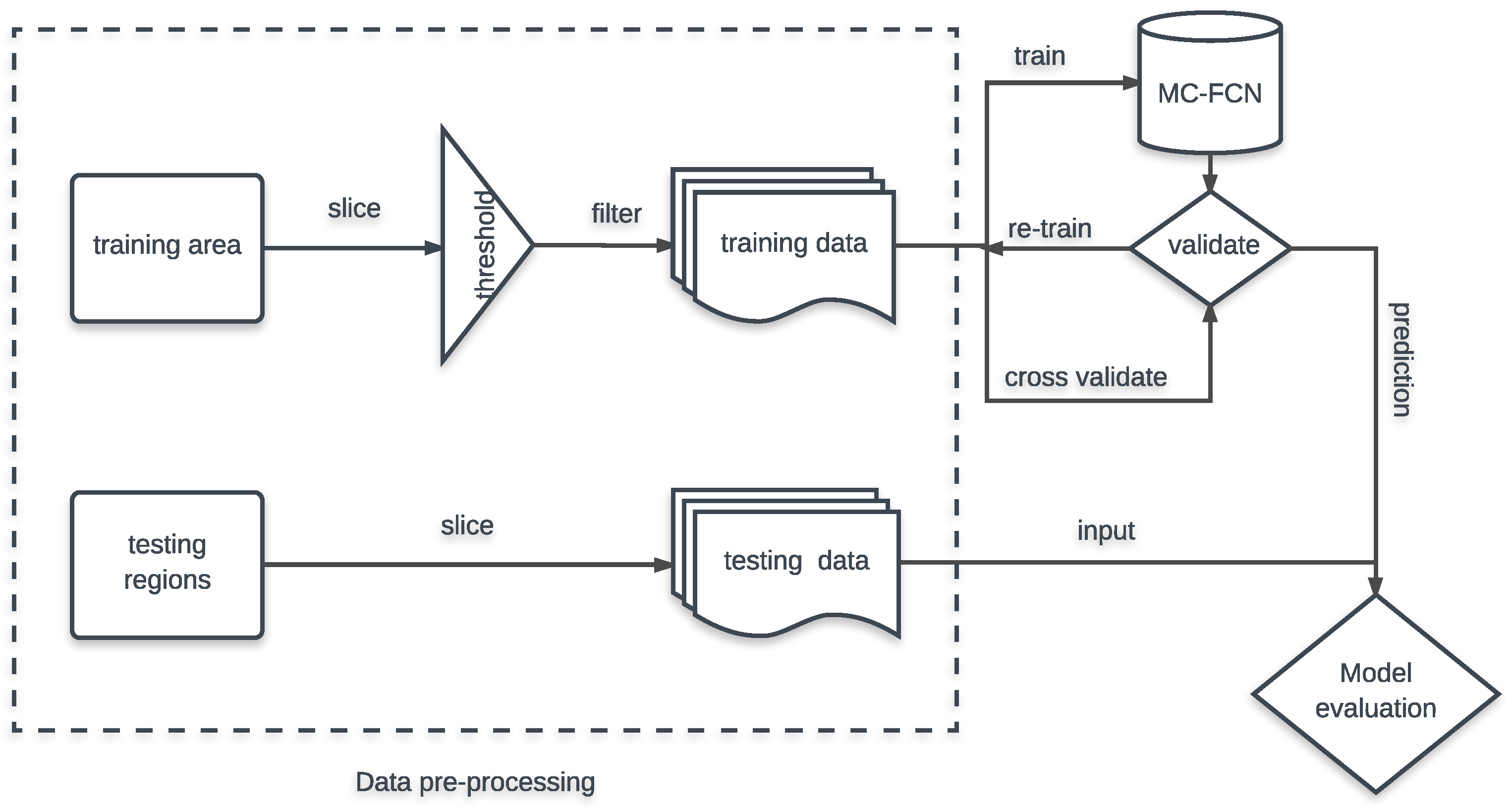
The classic FCN and U–Net model are adopted as the baseline deep-learning methods for comparison. In addition, as a representative classification method based on manually designed features, the AdaBoost classifier using HOG features (HOG–Ada for short) is also involved in the trials.

3.1. Qualitative Result Comparison

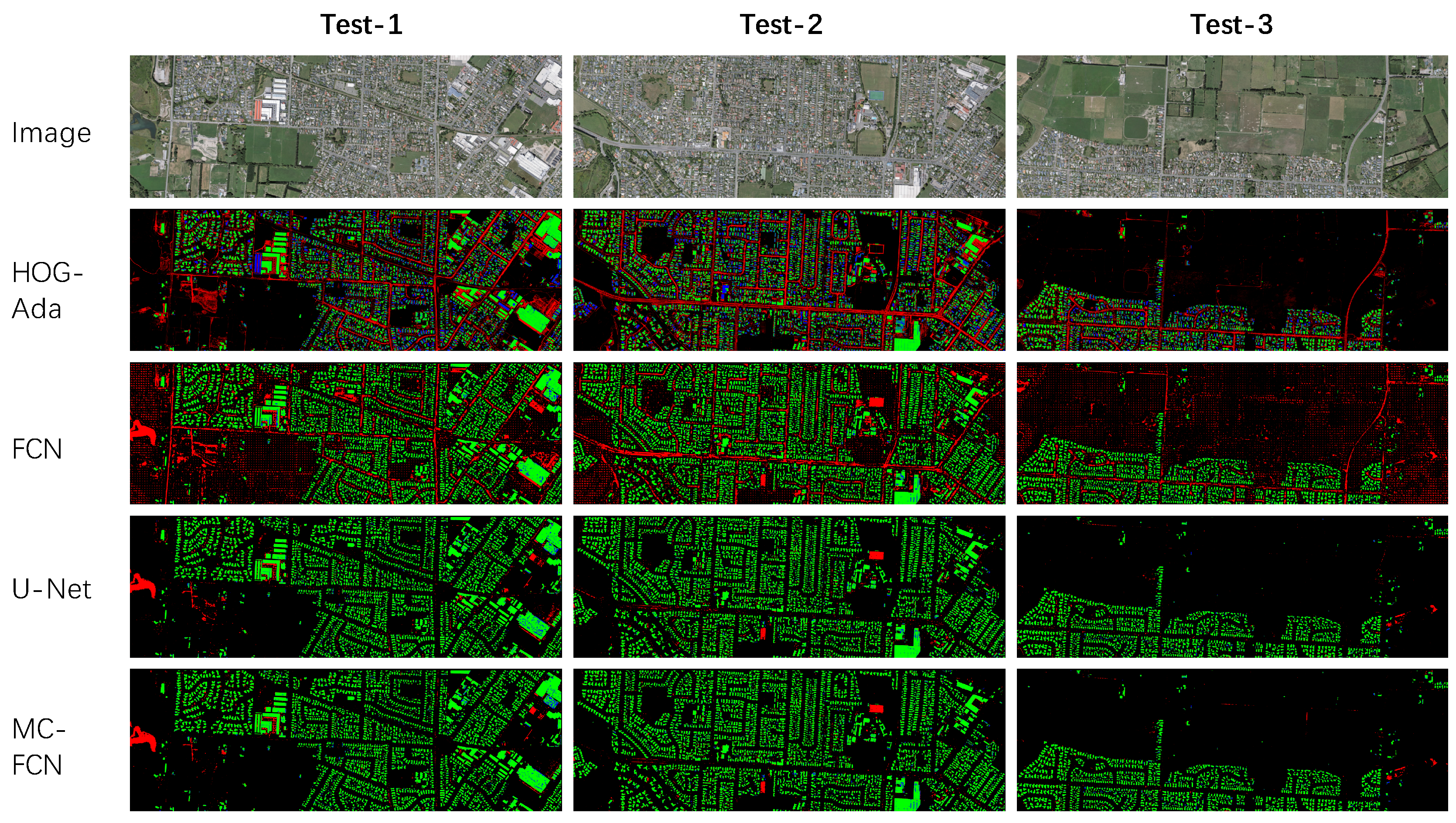
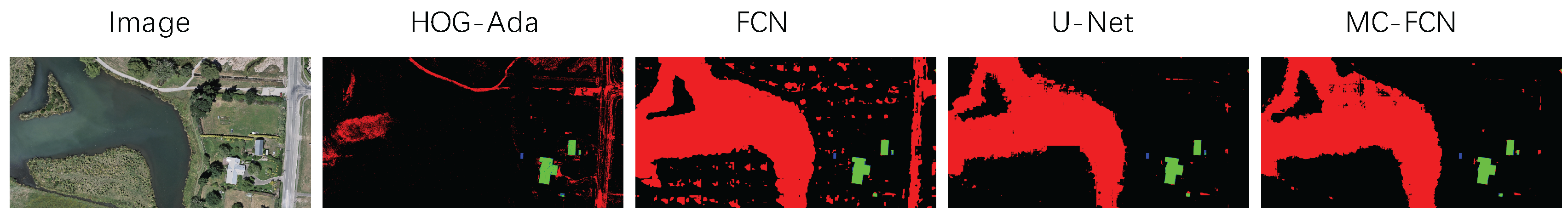
Figure 4 shows that the U–Net and MC–FCN methods are better than FCN, and significantly outperform the HOG–Ada method. In Test-1, HOG–Ada returns more false positives and false negatives than do the other CNN-based methods. However, in the left-middle corner of Test-1, where FCN, U–Net and MC–FCN misclassifies a small lake, HOG–Ada is still able to distinguish the lake with the help of textual features. In regions occupied by non-building backgrounds (Test-3), MC–FCN and U–Net show a significantly smaller number of false positives than other methods, while maintaining high completeness in building extraction. Similar comparison results can be observed from Test-2.

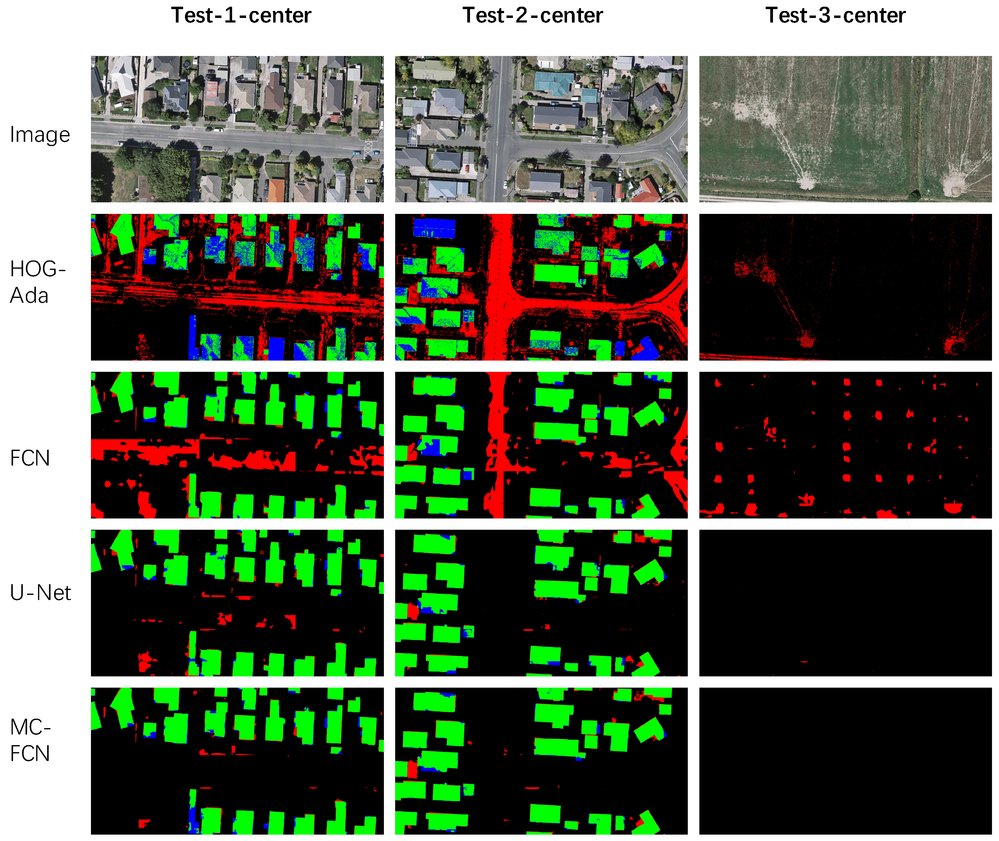
Figure 5 shows the enlarged segmentation results of the center patches from the Test-1, Test-2 and Test-3 regions. In general, the U–Net and MC–FCN methods significantly outperform the FCN and HOG–Ada methods. From rows 2 and 3, although the FCN method outperforms HOG–Ada in detecting buildings (in Test-1 and -2), it sometimes performs even worse in background recognition (in Test-3). From rows 4 and 5, especially in Test-1, MC–FCN returns a similar number of true positives but much fewer false positives than does U–Net for variant types of landmarks. The visual observation is consistent with quantitative comparison results of

Table 5. Comparison of performance of HOG–Ada, FCN, U–Net and MC–FCN in Test-1, Test-2 and Test-3 regions. For every test region, the highest values for different metrics are highlighted in bold.

Regions	Methods	Precison	Recall	Jaccard Index	Overall Accuracy	Kappa
Test-1	HOG–Ada	0.497	0.715	0.414	0.826	0.479
	FCN	0.613	0.935	0.588	0.888	0.672
	U–Net	0.869	0.928	0.815	0.964	0.875
	MC–FCN	0.892	0.937	0.841	0.968	0.895
Test-2	HOG–Ada	0.476	0.684	0.390	0.785	0.424
	FCN	0.671	0.934	0.641	0.894	0.713
	U–Net	0.897	0.935	0.844	0.965	0.893
	MC–FCN	0.916	0.938	0.863	0.971	0.908
Test-3	HOG–Ada	0.363	0.690	0.307	0.921	0.418
	FCN	0.356	0.925	0.342	0.919	0.425
	U–Net	0.826	0.903	0.762	0.987	0.855
	MC–FCN	0.862	0.908	0.794	0.989	0.877
Mean	HOG–Ada	0.445	0.696	0.307	0.844	0.414
	FCN	0.547	0.931	0.524	0.900	0.603
	U–Net	0.864	0.922	0.807	0.972	0.874
	MC–FCN	0.890	0.928	0.833	0.976	0.893

, which indicates that the MC–FCN model shows higher increments of precision rather than those of recall.

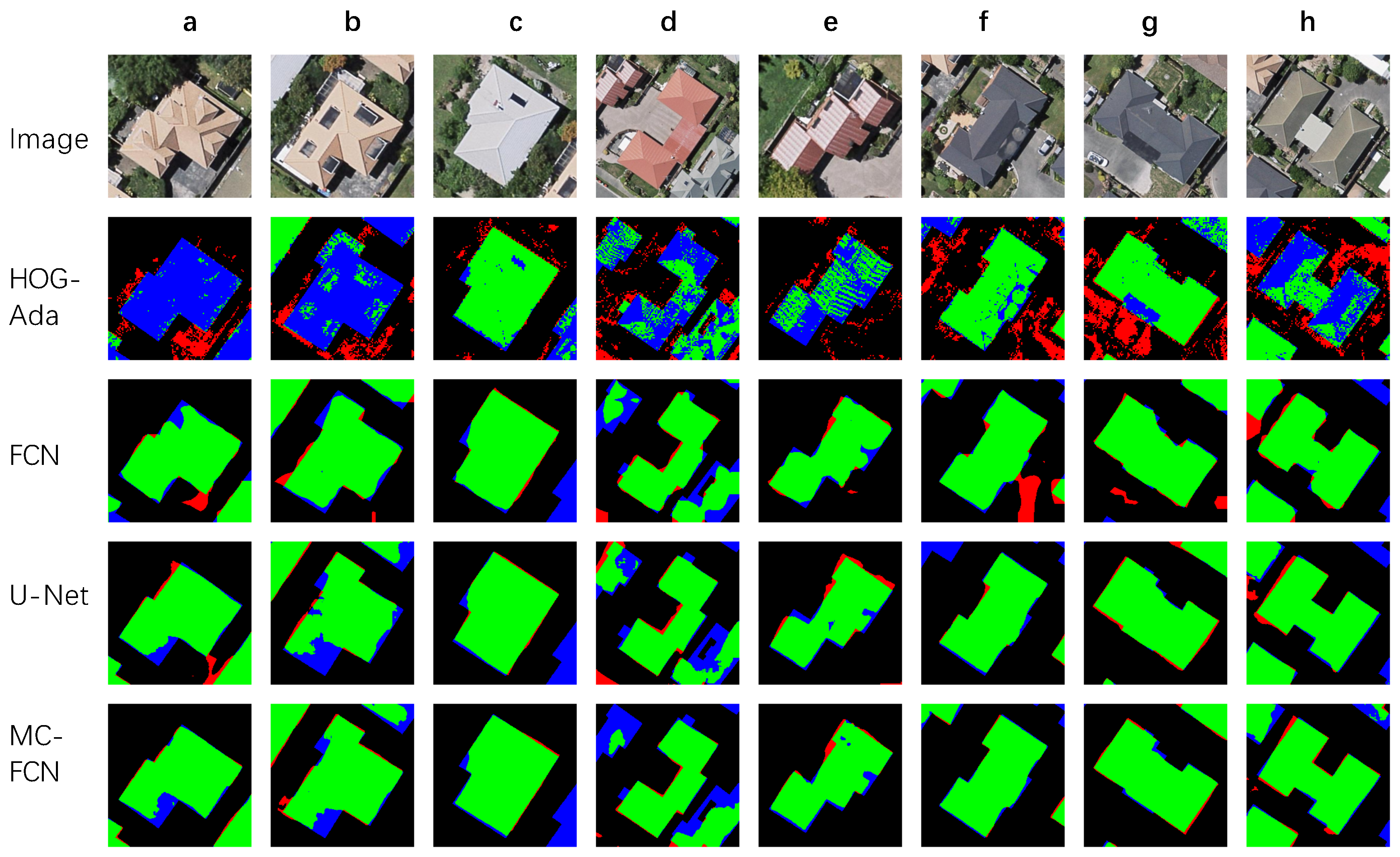
Since there is a large number of building samples in our experiment, in order to generate an objective reflection of the segmentation results, several samples are randomly selected for comparison first. Figure 6 presents the results of the samples from the Test-1, Test-2 and Test-3 regions generated by the HOG–Ada, FCN, U–Net and MC–FCN methods. In row 2, the HOG–Ada method is not able to extract buildings in most cases (in a, b, d, e and h). In c, f and g, although the HOG–Ada method correctly extracts major parts of the buildings, it still returns a significant number of false positives. In row 3, the FCN method shows quite good building extraction but still sometimes produces obvious false positives in the backgrounds (in a, f, g and h). From rows 4 and 5, the MC–FCN and U–Net methods present better performance in building extraction and noise reduction. When comparing the two, detectable improvements of MC–FCN over U–Net can be observed in restoring building boundaries (a, b, e, f and h) and suppressing false positives (a, e and h).

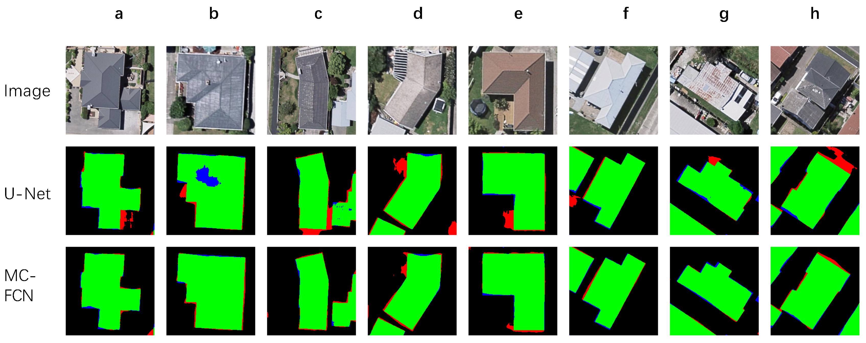
In order to further explore the improvements of our method over the classic U–Net, some representative samples were selected for additional comparison. Figure 7 shows the results of eight buildings generated by the U–Net and MC–FCN methods. The results indicate that both MC–FCN and U–Net methods are able to accurately extract the major parts of the buildings. Compared with the U–Net method, the MC–FCN method shows considerably fewer false positives, especially around the building edges (a, b, d, e and g) or in the gap areas between buildings (c, f and h). Interestingly, in some cases, the MC–FCN method also has better performance within the building boundaries (b and c).

3.2. Quantitative Result Comparison

Five commonly used metrics for image segmentation, including precision, recall, Jaccard index, overall accuracy and kappa coefficient, are used for quantitative evaluation in this study. Table 5 shows the comparison results of the four different methods for Test-1, Test-2 and Test-3 regions.

In the case of precision, the MC–FCN method holds the highest values among all testing regions, which indicates that our method performs well in suppressing false positives. Compared with U–Net, MC–FCN achieves 3.0% relative increase (0.890 vs. 0.864) on the mean value of precision. Particularly, in the test region with less residential area (Test-3), we achieve more significant improvement by gaining 4.4% relative increment of precision (0.862 vs. 0.826) over U–Net.

As for recall, the MC–FCN method presents the highest values of this value in Test-1 and Test-2 regions. Surprisingly, the FCN method outperforms the U–Net and MC–FCN methods in Test-3. Nonetheless, this slight advantage for FCN is far from being significant due to its low performance in other evaluation metrics. The difference between MC–FCN and U–Net in recall is not evident, although the former is slightly better than the latter in all three test regions.

For the Jaccard index, all methods except for HOG–Ada achieve their highest values in Test-2. Within all testing regions, the values of the Jaccard index from the MC–FCN method are the highest. The increments of MC–FCN over U–Net are more significant in regions with more complicated backgrounds (Test-1 and Test-3 regions). The increments of the Test-1, Test-2 and Test-3 regions are 0.026, 0.019 and 0.032, respectively. MC–FCN improves on the mean value of the Jaccard index of U–Net from 0.807 to 0.833 with a relative increase of about 3.2%.

As for overall accuracy, four methods obtain their highest values in the Test-3 region. Since overall accuracy only focuses on the correctness of pixel classification, even the smallest mean overall accuracy of the four methods reached 0.844 (HOG–Ada). The results of the MC–FCN method are the best among all regions.

As with the kappa coefficient, the four methods, except for the HOG–Ada, reached their highest values of the kappa coefficient in the Test-2 region. MC–FCN shows the highest kappa values across the Test-1, Test-2 and Test-3 regions. Compared with HOG–Ada, FCN and U–Net, the mean values of this metric increase were 0.453, 0.290 and 0.019, respectively.

3.3. Sensitivity Analysis of Constraints

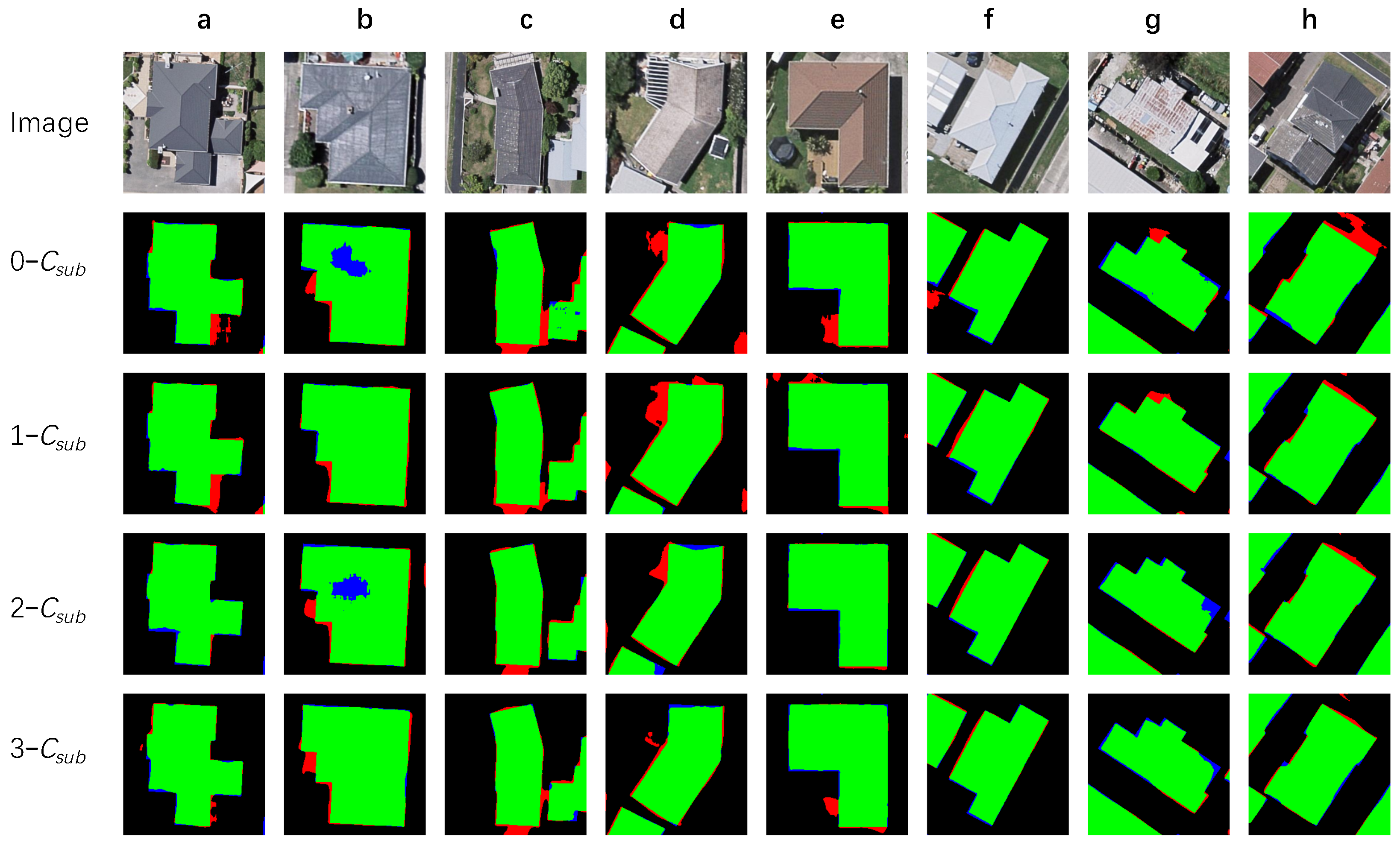
The sensitivity to the number of applied subconstraints is analyzed. Figure 8 presents the representative segmentation results from MC–FCN models with 0, 1, 2 or 3 subconstraints. Looking from top to bottom, MC–FCN models with more subconstraints result in slightly fewer false positives (a, d, f and h). However, in some cases, more subconstraints lead to more false negatives and weaker performance (b and g).

In

Table 6. Comparison of performance of MC–FCN models with variant numbers of subconstraints. The highest values for different metrics are highlighted in bold.

No. of ${\mathit{C}}_{\mathit{sub}}$	Precision	Recall	Jaccard Index	Overall Accuracy	Kappa
0	0.864	0.922	0.807	0.972	0.874
1	0.864	0.932	0.814	0.972	0.880
2	0.903	0.901	0.823	0.974	0.886
3	0.882	0.923	0.823	0.974	0.886

, the evaluation results of the MC–FCN models with 0, 1, 2 and 3 subconstraints are listed. The values of Jaccard index, overall accuracy or kappa coefficient indicate that having more constraints generally increases the performance of the MC–FCN, although models with two or three subconstraints hold consistent mean values of the three metrics. However, as for the imbalanced metrics, precision and recall show an inconsistent trend of increments, which implies that the model becomes unstable in controlling false predictions when the number of subconstraints increases.

Figure 9 shows the representative segmentation results from MC–FCN models with constraint combinations of $C_{main}$ only, $C_{main}+C_{sub1}$, $C_{main}+C_{sub2}$ or $C_{main}+C_{sub3}$. The MC–FCN models with constraint combinations of $C_{main}+C_{sub2}$ and $C_{main}+C_{sub3}$ have much fewer false positive, especially at building edges (a, b, e, g and h) or in the gaps between buildings (c).

Table 7. Comparison of performance of MC–FCN models with different constraint combinations. The highest values for different metrics are highlighted in bold.

Constraints	Precision	Recall	Jaccard Index	Overall Accuracy	Kappa
$C_{main}$	0.864	0.922	0.807	0.972	0.874
$C_{main}+C_{sub1}$	0.864	0.932	0.814	0.972	0.880
$C_{main}+C_{sub2}$	0.896	0.917	0.830	0.976	0.891
$C_{main}+C_{sub3}$	0.890	0.928	0.833	0.976	0.893

shows the evaluation results of the MC–FCN models with constraint combinations of $C_{main}$ only, $C_{main}+C_{sub1}$, $C_{main}+C_{sub2}$ or $C_{main}+C_{sub3}$. It turns out that the performance of the model with the constraint combination of $C_{main}+C_{sub3}$ is better than those of other combinations. Apparently, the better performance of this combination benefits from a good tradeoff between precision and recall.

3.4. Computational Efficiency

Considering the relatively closer performance, an efficiency comparison between different deep-learning methods was conducted. The algorithms of FCN, U–Net and MC–FCN were implemented in Keras using Tensorflow as backend and performed on a 64-bit Ubuntu system (ASUS: Beitou District, Taipei, Taiwan) equipped with NVIDIA GeForce GTX 1070 GPU (Nvidia: Santa Clara (HQ), CA, USA) graphic device with 8G byte graphic memory. During training, the Adam stochastic optimizer [42] with a learning rate of 0.001 was used. The difference of computational efficiency between these methods mainly lies in the time cost of the training process, which is generally proportional to the complexity of the model. The FCN, U–Net and the proposed MC–FCN models require 178.3, 365.7 and 372.1 min, respectively, for 100 epochs of iterations using the same training dataset. It can be concluded that MC–FCN gains 3.0% (0.833 vs. 0.807) and 2.2% (0.893 vs. 0.874) relative increments of Jaccard index and kappa coefficient, respectively, over U–Net with the cost of only 1.8% increment of model-training time; the extra time brings a cost-effective improvement of the segmentation performance.

4. Discussions

4.1. About the Proposed MC–FCN Model

The proposed MC–FCN model follows the basic structure of U–Net [29]. From the perspective of model design, our major improvement is applying a 1 × 1 convolution operation for the intermediate layers of the top-down feature pyramid to generate additional predictions, which enables multi-constraints on different spatial scales for the model during the training process. Although the effectiveness of multi-constraints applied on FCNs has been demonstrated by Xie et al. [30], their work was conducted based on the FCN framework for application of edge detection. However, in our study, targeting building segmentation from aerial images, the more effective U–Net architecture is adopted. Another related study has proven the usefulness of multi-scale prediction based on the feature pyramid [31]. However, compared with our approach, their study focused more on fusing the features extracted from different scales to achieve higher performance, and the multi-constraints were not explicitly applied on the intermediate layers in their model.

In the field of remote sensing, some studies on the detection of informal settlements [43] or buildings in rural areas [24,44] have demonstrated the potential of applying CNN architectures for high-accuracy automatic building detection. However, their patch-based CNN methods usually require large amounts of memory and computational capability, which limit the applicability of these methods to large areas. There are also other studies [45,46] that segment aerial imagery in an end-to-end fully convolutional manner, and these approaches significantly reduce the usage of memory and improve segmentation accuracy. However, their methods are built up by the classic FCN model, which simply upsamples intermediate layers (no skip connection) and leads to insufficient precision. The state-of-the-art U–Net model that we use for building segmentation shows better performance. More recently, by integrating the architecture of U–Net and the deep residual networks (ResNet) [47], Xu et al. achieved high performance in accurately extracting buildings from aerial imagery [48]. However, compared with our approach, they adopted infrared band data and the digital surface model besides RGB images to improve the accuracy. Meanwhile, multi-constraints applied on intermediate layers, which are proven effective in our MC–FCN model, were not considered in Xu et al.’s work.

4.2. Accuracies, Uncertainties and Limitations

As compared to the AdaBoost methods using hand-crafted feature descriptors (HOG–Ada), classic fully convolutional networks (FCNs) and the state-of-the-art fully convolutional model (U–Net), our MC–FCN model showed better performance in the evaluation metrics of the Jaccard index, overall accuracy and kappa coefficient. Particularly, the mean values of the kappa coefficient of the MC–FCN, U–Net, FCN and HOG–Ada methods are 0.893, 0.874, 0.603 and 0.440, respectively. Our MC–FCN method is better than the U–Net and FCN methods, and significantly outperforms the HOG–Ada method.

In the sensitivity analysis of the MC–FCN, when gradually increasing the number of subconstraints in ascending order, models with more subconstraints ($C_{sub}$) performed better. Also, when applying only one subconstraint along with the main constraint, different combinations led to different impacts on the performance. Specifically, the farther the $C_{main}$ – $C_{sub\ast }$ combination, the better the model performs. Another interesting finding is that the model with two constraints outperforms that with all four constraints. The increments of the Jaccard index and the kappa coefficient by the MC–FCN model with $C_{main}$ and $C_{sub3}$ reach 0.026 and 0.019, respectively, whereas these numbers are 0.015 and 0.012, respectively, in the case of the MC–FCN model with $C_{main},C_{sub1},C_{sub2}$ and $C_{sub3}$. This demonstrates that the improvement of the performance is affected more by the positions of the subconstraints rather than the number of them.

Previous applications of ResNet have shown that a deeper network is very likely to lead to better results. However, the effectiveness of applying multi-constraints on a deeper network remains uncertain for us. The model scales are determined by two important factors: the scale of data as well as the computational capability. Although a deeper neural network has greater representation capability, it is better to have a large-enough dataset for training in order to avoid overfitting. In our study, the overfitting problem is well handled when applying a relatively deep network. Meanwhile, the computational capability should also be considered because of efficiency requirements in the experiment. In this approach, when high accuracy was achieved, we fixed the number of layers due to limited computing resources.

In general, CNN-based methods, especially our proposed MC–FCN method, significantly outperform the HOG–Ada method in building extraction and background elimination. However, in the left-middle corner of Test-1 (see Figure 10), the CNN-based methods have a number of misclassified pixels, while the HOG–Ada method produces quite clean results with simple RGB and texture features extracted by the HOG descriptor. The ability to adaptively adjust the parameters by the feeding data is an advantage for the CNN method but can also sometimes be a limitation when there are insufficient training data. Recent research [49,50], which combines hand-crafted features and CNN-learned features, shows promising improvement. As a continuation of this work, additional data sources (e.g., more complicated background types), as well as the fusion of hand-crafted features and CNN-learned features, could be considered for improving this limitation.

5. Conclusions

In this research, a multi-constraint fully convolutional network (MC–FCN) was proposed to further improve the performance of the state-of-the-art U–Net model. With extra constraints applied on the intermediate layers, the proposed method presented more powerful ability in feature representation, leading to higher performance in building segmentation from aerial imagery. The experiment on an image dataset covering 18 km${}^2$ and more than 17,000 buildings indicated that our method performed well in building segmentation by achieving mean values of Jaccard index, overall accuracy and kappa coefficient at 0.833, 0.976 and 0.893, respectively. The proposed MC–FCN method significantly outperformed the classic FCN method and the adaptive boosting method using features extracted by the histogram of oriented gradients. In comparison with U–Net, MC–FCN showed a cost-effective improvement by gaining 3.2% (0.833 vs. 0.807) and 2.2% (0.893 vs. 0.874) relative increase of Jaccard index and kappa coefficient, respectively, with the cost of only 1.8% increment of the model-training time. Sensitivity analysis demonstrated that constraints applied on different levels of the feature pyramid have inconsistent impact on the model’s performance. In future studies, we will try to expand the training dataset and further optimize the network architecture to promote the generalization ability of the proposed model. Meanwhile, a deeper network and higher computing power will also be considered for this task.

References

1. Ma, L.; Li, M.; Ma, X.; Cheng, L.; Du, P.; Liu, Y. A review of supervised object-based land-cover image classification. ISPRS J. Photogramm. Remote Sens. 2017, 130, 277–293. [Google Scholar] [CrossRef]
2. Glasbey, C.A. An analysis of histogram-based thresholding algorithms. CVGIP Graph. Model. Image Process. 1993, 55, 532–537. [Google Scholar] [CrossRef]
3. Chen, J.S.; Huertas, A.; Medioni, G. Fast convolution with Laplacian-of-Gaussian masks. IEEE Trans. Pattern Anal. Mach. Intell. 1987, PAMI-9, 584–590. [Google Scholar] [CrossRef]
4. Kanopoulos, N.; Vasanthavada, N.; Baker, R.L. Design of an image edge detection filter using the Sobel operator. IEEE J. Solid-State Circ. 1988, 23, 358–367. [Google Scholar] [CrossRef]
5. Canny, J. A computational approach to edge detection. In Readings in Computer Vision; Elsevier: Amsterdam, The Netherlands, 1987; pp. 184–203. [Google Scholar]
6. Wu, Z.; Leahy, R. An optimal graph theoretic approach to data clustering: Theory and its application to image segmentation. IEEE Trans. Pattern Anal. Mach. Intell. 1993, 15, 1101–1113. [Google Scholar] [CrossRef]
7. Chuang, K.S.; Tzeng, H.L.; Chen, S.; Wu, J.; Chen, T.J. Fuzzy c-means clustering with spatial information for image segmentation. Comput. Med. Imaging Graph. 2006, 30, 9–15. [Google Scholar] [CrossRef] [PubMed]
8. Zhen, D.; Zhongshan, H.; Jingyu, Y.; Zhenming, T. FCM Algorithm for the Research of Intensity Image Segmentation. Acta Electron. Sin. 1997, 5, 39–43. [Google Scholar]
9. Pappas, T.N. An adaptive clustering algorithm for image segmentation. IEEE Trans. Signal Process. 1992, 40, 901–914. [Google Scholar] [CrossRef]
10. Tremeau, A.; Borel, N. A region growing and merging algorithm to color segmentation. Pattern Recognit. 1997, 30, 1191–1203. [Google Scholar] [CrossRef]
11. Ok, A.O. Automated detection of buildings from single VHR multispectral images using shadow information and graph cuts. ISPRS J. Photogramm. Remote Sens. 2013, 86, 21–40. [Google Scholar] [CrossRef]
12. Karantzalos, K.; Paragios, N. Recognition-driven two-dimensional competing priors toward automatic and accurate building detection. IEEE Trans. Geosci. Remote Sens. 2009, 47, 133–144. [Google Scholar] [CrossRef]
13. Li, M.; Zang, S.; Zhang, B.; Li, S.; Wu, C. A review of remote sensing image classification techniques: The role of spatio-contextual information. Eur. J. Remote Sens. 2014, 47, 389–411. [Google Scholar] [CrossRef]
14. Viola, P.; Jones, M. Rapid object detection using a boosted cascade of simple features. In Proceedings of the IEEE Computer Society Conference on Computer Vision and Pattern Recognition, Kauai, HI, USA, 8–14 December 2001; Volume 1. [Google Scholar]
15. Lowe, D.G. Object recognition from local scale-invariant features. In Proceedings of the Seventh IEEE International Conference on Computer Vision, Kerkyra, Greece, 20–27 September 1999; Volume 2, pp. 1150–1157. [Google Scholar]
16. Ojala, T.; Pietikainen, M.; Maenpaa, T. Multiresolution gray-scale and rotation invariant texture classification with local binary patterns. IEEE Trans. Pattern Anal. Mach. Intell. 2002, 24, 971–987. [Google Scholar] [CrossRef]
17. Dalal, N.; Triggs, B. Histograms of oriented gradients for human detection. In Proceedings of the Computer IEEE Computer Society Conference on Vision and Pattern Recognition, San Diego, CA, USA, 20–25 June 2005; Volume 1, pp. 886–893. [Google Scholar]
18. Inglada, J. Automatic recognition of man-made objects in high resolution optical remote sensing images by SVM classification of geometric image features. ISPRS J. Photogramm. Remote Sens. 2007, 62, 236–248. [Google Scholar] [CrossRef]
19. Aytekin, Ö.; Zöngür, U.; Halici, U. Texture-based airport runway detection. IEEE Geosci. Remote Sens. Lett. 2013, 10, 471–475. [Google Scholar] [CrossRef]
20. Dong, Y.; Du, B.; Zhang, L. Target detection based on random forest metric learning. IEEE J. Sel. Top. Appl. Earth Obs. Remote Sens. 2015, 8, 1830–1838. [Google Scholar] [CrossRef]
21. Li, E.; Femiani, J.; Xu, S.; Zhang, X.; Wonka, P. Robust rooftop extraction from visible band images using higher order CRF. IEEE Trans. Geosci. Remote Sens. 2015, 53, 4483–4495. [Google Scholar] [CrossRef]
22. LeCun, Y.; Bengio, Y. Convolutional networks for images, speech, and time series. In The Handbook of Brain Theory and Neural Networks; MIT Press: Cambridge, MA, USA, 1995; Volume 3361, p. 1995. [Google Scholar]
23. Ciresan, D.; Giusti, A.; Gambardella, L.M.; Schmidhuber, J. Deep neural networks segment neuronal membranes in electron microscopy images. In Advances in Neural Information Processing Systems; MIT Press: Cambridge, MA, USA, 2012; pp. 2843–2851. [Google Scholar]
24. Guo, Z.; Shao, X.; Xu, Y.; Miyazaki, H.; Ohira, W.; Shibasaki, R. Identification of village building via Google Earth images and supervised machine learning methods. Remote Sens. 2016, 8, 271. [Google Scholar] [CrossRef]
25. Kampffmeyer, M.; Salberg, A.B.; Jenssen, R. Semantic segmentation of small objects and modeling of uncertainty in urban remote sensing images using deep convolutional neural networks. In Proceedings of the IEEE Conference on Computer Vision and Pattern Recognition Workshops, Las Vegas, NV, USA, 26 June–1 July 2016; pp. 1–9. [Google Scholar]
26. Long, J.; Shelhamer, E.; Darrell, T. Fully convolutional networks for semantic segmentation. In Proceedings of the IEEE Conference on Computer Vision and Pattern Recognition, Boston, MA, USA, 7–12 June 2015; pp. 3431–3440. [Google Scholar]
27. Badrinarayanan, V.; Kendall, A.; Cipolla, R. Segnet: A deep convolutional encoder-decoder architecture for image segmentation. arXiv, 2015; arXiv:1511.00561. [Google Scholar]
28. Noh, H.; Hong, S.; Han, B. Learning deconvolution network for semantic segmentation. In Proceedings of the IEEE International Conference on Computer Vision, Washington, DC, USA, 3–7 December 2015; pp. 1520–1528. [Google Scholar]
29. Ronneberger, O.; Fischer, P.; Brox, T. U–Net: Convolutional networks for biomedical image segmentation. In Proceedings of the International Conference on Medical Image Computing and Computer-Assisted Intervention, Munich, Germany, 5–9 October 2015; pp. 234–241. [Google Scholar]
30. Xie, S.; Tu, Z. Holistically-nested edge detection. In Proceedings of the IEEE International Conference on Computer Vision, Washington, DC, USA, 7–13 December 2015; pp. 1395–1403. [Google Scholar]
31. Lin, T.Y.; Dollár, P.; Girshick, R.; He, K.; Hariharan, B.; Belongie, S. Feature pyramid networks for object detection. In Proceedings of the IEEE Conference on Computer Vision and Pattern Recognition (CVPR), Minneapolis, MN, USA, 17 June–22 June 2017; Volume 1, p. 4. [Google Scholar]
32. Polak, M.; Zhang, H.; Pi, M. An evaluation metric for image segmentation of multiple objects. Image Vis. Comput. 2009, 27, 1223–1227. [Google Scholar] [CrossRef]
33. Everingham, M.; Van Gool, L.; Williams, C.K.; Winn, J.; Zisserman, A. The pascal visual object classes (voc) challenge. Int. J. Comput. Vis. 2010, 88, 303–338. [Google Scholar] [CrossRef]
34. Carletta, J. Assessing agreement on classification tasks: The kappa statistic. Comput. Linguist. 1996, 22, 249–254. [Google Scholar]
35. Paisitkriangkrai, S.; Sherrah, J.; Janney, P.; Hengel, V.D. Effective semantic pixel labelling with convolutional networks and conditional random fields. In Proceedings of the IEEE Conference on Computer Vision and Pattern Recognition Workshops, Boston, MA, USA, 7–12 June 2015; pp. 36–43. [Google Scholar]
36. LeCun, Y.; Bottou, L.; Bengio, Y.; Haffner, P. Gradient-based learning applied to document recognition. Proc. IEEE 1998, 86, 2278–2324. [Google Scholar] [CrossRef]
37. Nair, V.; Hinton, G.E. Rectified linear units improve restricted boltzmann machines. In Proceedings of the 27th International Conference on Machine Learning (ICML-10), Haifa, Israel, 21–24 June 2010; pp. 807–814. [Google Scholar]
38. Nagi, J.; Ducatelle, F.; Di Caro, G.A.; Cireşan, D.; Meier, U.; Giusti, A.; Nagi, F.; Schmidhuber, J.; Gambardella, L.M. Max-pooling convolutional neural networks for vision-based hand gesture recognition. In Proceedings of the IEEE International Conference on Signal and Image Processing Applications (ICSIPA), Kuala Lumpur, Malaysia, 16–18 November 2011; pp. 342–347. [Google Scholar]
39. Novak, K. Rectification of digital imagery. Photogramm. Eng. Remote Sens. 1992, 58. [Google Scholar]
40. Shore, J.; Johnson, R. Properties of cross-entropy minimization. IEEE Trans. Inf. Theory 1981, 27, 472–482. [Google Scholar] [CrossRef]
41. Ioffe, S.; Szegedy, C. Batch normalization: Accelerating deep network training by reducing internal covariate shift. In Proceedings of the International Conference on Machine Learning, Lille, France, 6–11 July 2015; pp. 448–456. [Google Scholar]
42. Kingma, D.P.; Ba, J. Adam: A method for stochastic optimization. arXiv, 2014; arXiv:1412.6980. [Google Scholar]
43. Mboga, N.; Persello, C.; Bergado, J.R.; Stein, A. Detection of Informal Settlements from VHR Images Using Convolutional Neural Networks. Remote Sens. 2017, 9, 1106. [Google Scholar] [CrossRef]
44. Guo, Z.; Chen, Q.; Wu, G.; Xu, Y.; Shibasaki, R.; Shao, X. Village Building Identification Based on Ensemble Convolutional Neural Networks. Sensors 2017, 17, 2487. [Google Scholar] [CrossRef] [PubMed]
45. Maggiori, E.; Tarabalka, Y.; Charpiat, G.; Alliez, P. Convolutional neural networks for large-scale remote-sensing image classification. IEEE Trans. Geosci. Remote Sens. 2017, 55, 645–657. [Google Scholar] [CrossRef]
46. Maggiori, E.; Tarabalka, Y.; Charpiat, G.; Alliez, P. Fully convolutional networkss for remote sensing image classification. In Proceedings of the IEEE International Conference on Geoscience and Remote Sensing Symposium (IGARSS), Beijing, China, 10–15 July 2016; pp. 5071–5074. [Google Scholar]
47. He, K.; Zhang, X.; Ren, S.; Sun, J. Deep residual learning for image recognition. In Proceedings of the IEEE Conference on Computer Vision and Pattern Recognition, Las Vegas, NV, USA, 26 June–1 July 2016; pp. 770–778. [Google Scholar]
48. Xu, Y.; Wu, L.; Xie, Z.; Chen, Z. Building Extraction in Very High Resolution Remote Sensing Imagery Using Deep Learning and Guided Filters. Remote Sens. 2018, 10, 144. [Google Scholar] [CrossRef]
49. Jin, L.; Gao, S.; Li, Z.; Tang, J. Hand-crafted features or machine learnt features? together they improve RGB-D object recognition. In Proceedings of the IEEE International Symposium on Multimedia (ISM), Taichung, Taiwan, 10–12 December 2014; pp. 311–319. [Google Scholar]
50. Wu, S.; Chen, Y.C.; Li, X.; Wu, A.C.; You, J.J.; Zheng, W.S. An enhanced deep feature representation for person re-identification. In Proceedings of the IEEE Winter Conference on Applications of Computer Vision (WACV), Lake Placid, NY, USA, 7–10 March 2016; pp. 1–8. [Google Scholar]
Figure 1. Aerial imagery of the study area. The area covers 18 km 2 of residential area, factories or farms in New Zealand, and is located from –43 ° 28′(N) to –43 ° 30′(S) and 172 ° 34′(W) to 172 ° 38′(E).
Remotesensing 10 00407 g001
Figure 2. Scheme of the experiment. The MC–FCNs are trained and cross-validated using training dataset, then evaluated by the testing dataset.
Remotesensing 10 00407 g002
Figure 3. Network architecture of the proposed multi-constraint fully convolutional network (MC–FCN). The MC–FCN model adopts the basic structure of U–Net and adds three extra multi-scale constraints between upsampled layers and their corresponding ground truths.
Remotesensing 10 00407 g003
Figure 4. Segmentation results of HOG–Ada, FCN, U–Net and MC–FCN for the Test-1, Test-2 and Test-3 regions. The green, red, blue and black pixels of the maps represent the predictions of true positive, false positive, false negative and true negative, respectively.
Remotesensing 10 00407 g004
Figure 5. Center patches of segmentation results of Test-1, Test-2 and Test-3 regions. The green, red, blue and black pixels of the maps represent the predictions of true positive, false positive, false negative and true negative, respectively.
Remotesensing 10 00407 g005
Figure 6. Segmentation results of randomly sampled buildings from the HOG–Ada, FCN, U–Net and MC–FCN methods. Images within columns (ah) are sampled buildings from Test-1, Test-2 and Test-3 regions. The green, red and blue channels of results represent true positive, false positive and false negative predictions, respectively, of every pixel.
Remotesensing 10 00407 g006
Figure 7. Representative results of building segmentation through the U–Net and MC–FCN methods. The green, red and blue channels of results represent true positive, false positive and false negative predictions, respectively, of every pixel.
Remotesensing 10 00407 g007
Figure 8. Representative results of building segmentation through MC–FCN models with variant numbers of subconstraints. The green, red and blue channels of results represent true positive, false positive and false negative predictions, respectively, of every pixel.
Remotesensing 10 00407 g008
Figure 9. Representative results of segmented buildings from MC–FCN models with different constraint combinations. The green, red and blue channels of results represent true positive, false positive and false negative predictions, respectively, of every pixel.
Remotesensing 10 00407 g009
Figure 10. Zoomed-in image of the middle-left corner of the Test-1 region in Figure 4, where a small lake was misclassified as a building by all CNN-based methods. The green, red, blue and black pixels denote the predictions of true positive, false positive, false negative and true negative, respectively.
Remotesensing 10 00407 g010