Discriminant Analysis with Graph Learning for Hyperspectral Image Classification

Abstract

Linear Discriminant Analysis (LDA) is a widely-used technique for dimensionality reduction, and has been applied in many practical applications, such as hyperspectral image classification. Traditional LDA assumes that the data obeys the Gaussian distribution. However, in real-world situations, the high-dimensional data may be with various kinds of distributions, which restricts the performance of LDA. To reduce this problem, we propose the Discriminant Analysis with Graph Learning (DAGL) method in this paper. Without any assumption on the data distribution, the proposed method learns the local data relationship adaptively during the optimization. The main contributions of this research are threefold: (1) the local data manifold is captured by learning the data graph adaptively in the subspace; (2) the spatial information within the hyperspectral image is utilized with a regularization term; and (3) an efficient algorithm is designed to optimize the proposed problem with proved convergence. Experimental results on hyperspectral image datasets show that promising performance of the proposed method, and validates its superiority over the state-of-the-art.

1. Introduction

Hyperspectral Image (HSI) provides hundreds of spectral bands for each pixel and conveys a lot of surface information. Hyperspectral image classification aims to distinguish the land-cover types of each pixel, and the spectral bands are considered as features. However, the great number of bands significantly increases the computational complexity [1]. Moreover, some bands are highly correlated, leading to the feature redundancy problem. Consequently, it is critical to perform dimensionality reduction before classification. The goal of dimensionality reduction is to project the original data into a low-dimensional subspace while preserving the valuable information.

Dimensionality reduction techniques can be roughly classified into two categories: feature selection [2,3] and feature extraction [4,5,6,7,8,9]. Feature selection methods select the most relevant feature subset from the original feature space, while feature extraction methods exploit the low-dimensional subspace that contains valuable information. Compared to feature selection, feature extraction is able to create meaningful features through the transformation of the original ones. Consequently, plenty of techniques have been put forward on feature extraction [9,10,11,12,13]. Principal Component Analysis (PCA) [14] and Linear Discriminant Analysis (LDA) [15] are the most popular feature extraction methods. PCA learns the feature subspace by maximizing the variance of the feature matrix. While LDA learns a linear transformation that minimizes the within-class distance and maximizes the between-class discrepancy. In this research, we mainly focus on LDA because it is able to use the prior knowledge and shows better performance in real-world applications [11].

Though achieving good performance in many tasks, LDA has four major drawbacks on processing HSI data. Firstly, LDA suffers from the ill-posed problem [12]. LDA needs to compute the inverse matrix of the within-class scatter ${\mathbf{S}}_w$. When the data dimensionality exceeds the number of training samples, ${\mathbf{S}}_w$ is irreversible. Thus, LDA cannot handle the HSI data with great number of spectral bands. Secondly, the feature dimensionality reduced by LDA is less than the class number, namely over-reducing problem [13]. Taking the Kennedy Space Center (KSC) dataset [16] for example, the class number is thirteen, and the rank of the between-class scatter ${\mathbf{S}}_b$ is at most twelve. Thus, LDA could find at most twelve projection directions, which may be insufficient for retaining the useful information. Thirdly, LDA neglects the spatial smoothness. In HSIs, the pixels within a spatial neighborhood region usually belong to the same class. However, LDA just focuses on the pixels’ distances in the feature space, and ignores the spatial aspect. Fourthly, LDA assumes that the data samples are Gaussian-distributed, and share equal covariances in all the classes. However, HSI data seldom obeys the Gaussian distribution [17], and the local data structure may be inconsistent with the global structure. Therefore, LDA is unable to find the local classification boundary for the HSI data.

In the past few decades, many variants of the original LDA are proposed, trying to enhance its performance from different views. Bandos et al. [18] proposed the Regularized LDA (RLDA), which employs a regularized within-class scatter to tackle the ill-posed problem. Kumar and Agrawal [19] presented the two-dimensional exponential discriminant analysis for data with small sample size. The Semi-supervised Discriminant Analysis (SDA) method [20] utilizes the unlabelled data to extend the training set. Wan et al. [13] and Nie et al. [10] developed the full rank between-class scatter matrix to mitigate the over-reducing problem. To enforce the spatial consistency, Yuan et al. [21] and Wang et al. [22] constructed a scatter matrix from a small neighborhood, and took it as a regularization term. With the above methods, the ill-posed and over-reducing problem are alleviated, and the spatial correlation between pixels can be preserved. However, the exploration of the local data structure remains to be an open issue. Some graph-based methods [10,11,23,24] defined the scatter matrices according to the predefined affinity graph, which may be seriously affected by the noise. Ly et al. [25] performed graph learning and discriminant analysis separately, so the data graph is also fixed during the optimization. Recently, Wang et al. [9] and Wu et al. [26] proposed to learn the data graph in the subspace. However, they neglect the similar samples from different classes, which largely determine the classification boundary.

In this work, we propose a new method for supervised dimensionality reduction, termed as Discriminant Analysis with Graph Learning (DAGL). In order to exploit the data structure, the proposed method learns the data graph adaptively during learning of transformation matrix. Furthermore, to guarantee the spatial smoothness, the samples within a small region are encouraged to share the same class label. With the proposed objective function, the proposed method does not have the ill-posed and over-reducing problem. The contributions made in paper are summarized as follows:

(1)

The affinity graph is built according to the samples’ distances in the subspace, so the local data structure is captured adaptively.

(2)

The proposed formulation perceives the spatial correlation within HSI data, and avoids the ill-posed and over-reducing problem naturally.

(3)

An alternative optimization algorithm is developed to solve the proposed problem, and its convergence is proved experimentally.

2. Linear Discriminant Analysis Revisited

In this section, the Linear Discriminant Analysis is briefly reviewed as the preliminary. Given an input data matrix $\mathbf{X}=[{\mathbf{x}}_1,{\mathbf{x}}_2,\cdots ,{\mathbf{x}}_n]\in {\mathbb{R}}^{d\times n}$ (d is the data dimensionality and n is the number of samples), LDA defines the between-class scatter ${\mathbf{S}}_b$ and within-class scatter ${\mathbf{S}}_w$ as

$$\begin{array}{c}{\mathbf{S}}_b={\displaystyle \sum _{k=1}^c}{n}_k({\mu }_k-\mu ){({\mu }_k-\mu )}^T,\hfill \\ {\mathbf{S}}_w={\displaystyle \sum _{k=1}^c}{\displaystyle \sum _{{\mathbf{x}}_i\in k}}({\mathbf{x}}_i-{\mu }_k){({\mathbf{x}}_i-{\mu }_k)}^T,\hfill \end{array}$$

(1)

where $n_k$ is the sample number in class k, c is the class number, ${\mu }_k$ is the mean of samples in class k and $\mu$ is the mean of all the samples. With the above definitions, LDA aims to learn a linear transformation $\mathbf{W}\in {\mathbb{R}}^{d\times m}(m\ll d)$, which maximizes the between-class difference while minimizing the within-class separation:

$$\underset{\mathbf{W}}{max}\mathrm{Tr}\left(\frac{{\mathbf{W}}^T{\mathbf{S}}_b\mathbf{W}}{{\mathbf{W}}^T{\mathbf{S}}_w\mathbf{W}}\right),$$

(2)

where $\mathrm{Tr}\left(\right)$ indicates the trace operator. With the optimal transformation ${\mathbf{W}}^{*}$, data sample ${\mathbf{x}}_i$ can be projected to a m-dimensional feature vector ${\mathbf{W}}^{*T}{\mathbf{x}}_i$.

As shown in Equation (1), LDA assumes that the data distribution is Gaussian and the between-class divergence can be reflected by the subtraction of the mean. This assumption is unsuitable for HSI data, and makes LDA insensitive to the local manifold.

3. Discriminant Analysis with Graph Learning

In this section, the Discriminant Analysis with Graph Learning (DAGL) method is introduced, and an optimization method is proposed to get the optimal solution.

3.1. Graph Learning

In real-world tasks, such as HSI classification, the local manifold may be inconsistent with the global structure. Thus, it is necessary to take the local data relationship into consideration.

In the past few decades, numerous algorithms are proposed to explore the data structure. Some of them [27,28,29,30] first construct an affinity graph with various kernels (Gaussian kernel, linear kernel, 0–1 weighting), and then perform clustering or classification according to the spectral of the predefined graph. However, the choice of kernel scales and categories is still an open issue. Therefore, the graph learning methods [25,31,32,33,34,35] are developed to learn the data graph automatically. One of the most popular graph learning techniques is Sparse Representation [31,32], which aims to learn a sparse graph from the original data. Spare Representation assumes that a data sample can be roughly represented by the linear combination of the others. Defining a coefficient matrix $\mathbf{S}\in {\mathbb{R}}^{n\times n}$, the optimal $\mathbf{S}$ should minimize the reconstruction error as follows:

$$\begin{array}{c}\underset{\mathbf{S}}{min}\sum _{j=1}^n\left|\right|{\mathbf{x}}_j-\sum _{i\ne j}{\mathbf{x}}_i{\mathbf{S}}_{ij}{\left|\right|}_2^2\hfill \\ =\underset{\mathbf{S}}{min}\left|\right|\mathbf{X}-{\mathbf{XS}\left|\right|}_F^2,\hfill \\ s.t.\sum _{i=1}^n{\mathbf{S}}_{ij}=1,\mathbf{S}\ge 0.\hfill \end{array}$$

(3)

If ${\mathbf{x}}_i$ and ${\mathbf{x}}_j$ are similar, ${\mathbf{S}}_{ij}$ will be large. Thus, $\mathbf{S}$ can be considered as the affinity graph.

3.2. Methodology

As shown in Equation (3), Sparse Representation exploits the data relationship in the original data space, and the data noise may affect the graph quality adversely. To reduce this problem, we propose to adjust the data graph during the discriminant analysis, which yields the following formula:

$$\begin{array}{c}\underset{\mathbf{W},\mathbf{S}}{min}\frac{{\displaystyle \sum _{k=1}^c}{\displaystyle \sum _{x_i,x_j\in k}}\left|\right|{\mathbf{W}}^T({\mathbf{x}}_i-{\mathbf{x}}_j){\left|\right|}_2^2{\mathbf{S}}_{ij}^2}{{\displaystyle \sum _{k=1}^c}{\displaystyle \sum _{x_i\in k,x_j\notin k}}\left|\right|{\mathbf{W}}^T({\mathbf{x}}_i-{\mathbf{x}}_j){\left|\right|}_2^2{\mathbf{S}}_{ij}^2}+\alpha \left|\right|\mathbf{X}-{\mathbf{XS}\left|\right|}_F^2,\hfill \\ s.t.{\mathbf{W}}^T\mathbf{W}=\mathbf{I},{\displaystyle \sum _{i=1}^n}{\mathbf{S}}_{ij}=1,\mathbf{S}\ge 0,\hfill \end{array}$$

(4)

where $\mathbf{I}\in {\mathbb{R}}^{m\times m}$ is the identity matrix, and $\alpha$ is a parameter. When the linear transformation $\mathbf{W}$ is learned, the first term of problem (4) enforces ${\mathbf{S}}_{ij}$ to be small/large for the within/between-class samples with large transformed distances. In this way, the data graph is optimized in the subspace. Similarly, when $\mathbf{S}$ is fixed, the transformed distance ${\mathbf{W}}^T\left|\right|{\mathbf{x}}_i-{\mathbf{x}}_j{\left|\right|}_2^2$ will be small/large for the within/between-class samples with large ${\mathbf{S}}_{ij}$. Consequently, the within-/between-class similar samples are ensured to be close/far away in the transformed subspace. However, it is difficult to optimize problem (4) directly because $\mathbf{S}$ is involved in both the numerator and denominator of the first term. Supposing the minimum value of the first term is $\gamma$, the optimal $\mathbf{W}$ and $\mathbf{S}$ should make the value of ${\displaystyle \sum _{k=1}^c}{\displaystyle \sum _{x_i,x_j\in k}}\left|\right|{\mathbf{W}}^T({\mathbf{x}}_i-{\mathbf{x}}_j){\left|\right|}_2^2{\mathbf{S}}_{ij}^2-\gamma {\displaystyle \sum _{k=1}^c}{\displaystyle \sum _{x_i\in k,x_j\notin k}}\left|\right|{\mathbf{W}}^T({\mathbf{x}}_i-{\mathbf{x}}_j){\left|\right|}_2^2{\mathbf{S}}_{ij}^2$ to be close to 0. Thus, problem (4) is equivalent to the following formula:

$$\begin{array}{c}\underset{\mathbf{W},\mathbf{S}}{min}\sum _{k=1}^c\sum _{x_i,x_j\in k}\left|\right|{\mathbf{W}}^T({\mathbf{x}}_i-{\mathbf{x}}_j){\left|\right|}_2^2{\mathbf{S}}_{ij}^2-\gamma \sum _{k=1}^c\sum _{x_i\in k,x_j\notin k}\left|\right|{\mathbf{W}}^T({\mathbf{x}}_i-{\mathbf{x}}_j){\left|\right|}_2^2{\mathbf{S}}_{ij}^2+\alpha \left|\right|\mathbf{X}-{\mathbf{XS}\left|\right|}_F^2,\hfill \\ s.t.{\mathbf{W}}^T\mathbf{W}=\mathbf{I},\sum _{i=1}^n{\mathbf{S}}_{ij}=1,\mathbf{S}\ge 0,\hfill \end{array}$$

(5)

where $\gamma$ can be set as a small value. Denoting a class indicator matrix $\mathbf{Z}\in {\mathbb{R}}^{n\times n}$ as

$${\mathbf{Z}}_{ij}=\left\{\begin{array}{c}1,\mathrm{if}{\mathbf{x}}_i\mathrm{and}{\mathbf{x}}_j\mathrm{are}\mathrm{from}\mathrm{the}\mathrm{same}\mathrm{class},\hfill \\ -\gamma ,\mathrm{else}\hfill \end{array}\right.$$

(6)

problem (5) can be simplified into

$$\begin{array}{c}\underset{\mathbf{W},\mathbf{S}}{min}\sum _{i,j=1}^n\left|\right|{\mathbf{W}}^T({\mathbf{x}}_i-{\mathbf{x}}_j){\left|\right|}_2^2{\mathbf{S}}_{ij}^2{\mathbf{Z}}_{ij}+\alpha \left|\right|\mathbf{X}-{\mathbf{XS}\left|\right|}_F^2,\hfill \\ s.t.{\mathbf{W}}^T\mathbf{W}=\mathbf{I},\sum _{i=1}^n{\mathbf{S}}_{ij}=1,\mathbf{S}\ge 0.\hfill \end{array}$$

(7)

In HSI data, the pixels within a small region may be highly correlated and belong to the same class. The spatial information is essential for an accurate classification. Given a test sample $\mathbf{t}\in {\mathbb{R}}^{d\times 1}$, we find its surroundings within a $r\times r$ region, and denote them as $[{\mathbf{t}}_1,{\mathbf{t}}_2,\cdots ,{\mathbf{t}}_{r^2-1}]$. For these samples, we encourage them to be close to each other in the desired subspace, which yields the following problem

$$\underset{\mathbf{W}}{min}\sum _{i,j=1}^{r^2-1}{\mathbf{W}}^T\left|\right|{\mathbf{t}}_i-{\mathbf{t}}_j{\left|\right|}_2^2.$$

(8)

Problem (8) can be further reduced to

$$\underset{\mathbf{W}}{min}\mathrm{Tr}\left({\mathbf{W}}^T{\tilde{\mathbf{S}}}_t\mathbf{W}\right),$$

(9)

where

$${\tilde{\mathbf{S}}}_t=\sum _{i,j=1}^{r^2-1}({\mathbf{t}}_i-{\mathbf{t}}_j){({\mathbf{t}}_i-{\mathbf{t}}_j)}^T.$$

(10)

Finally, by integrating problems (7) and (9) together, we have the objective function of the proposed DAGL method:

$$\begin{array}{c}\underset{\mathbf{W},\mathbf{S}}{min}\sum _{i,j=1}^n\left|\right|{\mathbf{W}}^T({\mathbf{x}}_i-{\mathbf{x}}_j){\left|\right|}_2^2{\mathbf{S}}_{ij}^2{\mathbf{Z}}_{ij}+\alpha \left|\right|\mathbf{X}-{\mathbf{XS}\left|\right|}_F^2+\beta \mathrm{Tr}\left({\mathbf{W}}^T{\tilde{\mathbf{S}}}_t\mathbf{W}\right),\hfill \\ s.t.{\mathbf{W}}^T\mathbf{W}=\mathbf{I},\sum _{i=1}^n{\mathbf{S}}_{ij}=1,\mathbf{S}\ge 0,\hfill \end{array}$$

(11)

where $\alpha$ and $\beta$ are parameters. Since DAGL does not need to calculate the inverse matrix of within-class scatter, the ill-posed problem is avoided naturally. In addition, the projected dimensionality m can be any value less than d, so the over-reducing problem does not occur. With the proposed objective function, the local data relationship is investigated, and the spatial correlation between the pixels is also captured.

3.3. Optimization Algorithm

Problem (11) involves two variables to be optimized, so we consider to fix one and update another one iteratively. The data graph $\mathbf{S}$ is firstly initialized with an efficient method [33].

When $\mathbf{S}$ is fixed, problem (11) becomes

$$\begin{array}{c}\underset{\mathbf{W}}{min}\sum _{i,j=1}^n\left|\right|{\mathbf{W}}^T({\mathbf{x}}_i-{\mathbf{x}}_j){\left|\right|}_2^2{\mathbf{S}}_{ij}^2{\mathbf{Z}}_{ij}+\beta \mathrm{Tr}\left({\mathbf{W}}^T{\tilde{\mathbf{S}}}_t\mathbf{W}\right),\hfill \\ s.t.{\mathbf{W}}^T\mathbf{W}=\mathbf{I}.\hfill \end{array}$$

(12)

Denoting a scatter matrix ${\tilde{\mathbf{S}}}_z$ as

$${\tilde{\mathbf{S}}}_z=\sum _{i,j=1}^n({\mathbf{x}}_i-{\mathbf{x}}_j){({\mathbf{x}}_i-{\mathbf{x}}_j)}^T{\mathbf{S}}_{ij}^2{\mathbf{Z}}_{ij},$$

(13)

problem (12) is converted into

$$\underset{{\mathbf{W}}^T\mathbf{W}=I}{min}\mathrm{Tr}[{\mathbf{W}}^T({\tilde{\mathbf{S}}}_z+\beta {\tilde{\mathbf{S}}}_t)\mathbf{W}].$$

(14)

According to the spectral clustering [36], the optimal $\mathbf{W}$ for problem (14) is formed by the m eigenvectors of matrix $({\tilde{\mathbf{S}}}_z+\beta {\tilde{\mathbf{S}}}_t)$ corresponding to the m smallest eigenvalues.

When $\mathbf{W}$ is fixed, by removing the irrelevant terms, problem (11) is transformed into

$$\begin{array}{c}\underset{\mathbf{W},\mathbf{S}}{min}\sum _{i,j=1}^n\left|\right|{\mathbf{W}}^T({\mathbf{x}}_i-{\mathbf{x}}_j){\left|\right|}_2^2{\mathbf{S}}_{ij}^2{\mathbf{Z}}_{ij}+\alpha \left|\right|\mathbf{X}-{\mathbf{XS}\left|\right|}_F^2,\hfill \\ s.t.\sum _{i=1}^n{\mathbf{S}}_{ij}=1,\mathbf{S}\ge 0.\hfill \end{array}$$

(15)

Fixing the diagonal elements in $\mathbf{S}$ as 0, the above problem is equivalent to

$$\begin{array}{c}\underset{\mathbf{W},\mathbf{S}}{min}\sum _{i,j=1}^n\left|\right|{\mathbf{W}}^T({\mathbf{x}}_i-{\mathbf{x}}_j){\left|\right|}_2^2{\mathbf{S}}_{ij}^2{\mathbf{Z}}_{ij}+\alpha \sum _{j=1}^n\left|\right|{\mathbf{x}}_j-\mathbf{X}{\mathbf{s}}_j{\left|\right|}_2^2,\hfill \\ s.t.\sum _{i=1}^n{\mathbf{S}}_{ij}=1,\mathbf{S}\ge 0,\hfill \end{array}$$

(16)

where ${\mathbf{s}}_j\in {\mathbb{R}}^{n\times 1}$ is the j-th column of $\mathbf{S}$. Since the ${\mathbf{s}}_j$ is independent between different j, we can solve the following problem for each j:

$$\begin{array}{c}\underset{\mathbf{W},\mathbf{S}}{min}\sum _{i=1}^n\left|\right|{\mathbf{W}}^T({\mathbf{x}}_i-{\mathbf{x}}_j){\left|\right|}_2^2{\mathbf{S}}_{ij}^2{\mathbf{Z}}_{ij}+\alpha \left|\right|{\mathbf{x}}_j-\mathbf{X}{\mathbf{s}}_j{\left|\right|}_2^2,\hfill \\ s.t.\sum _{i=1}^n{\mathbf{S}}_{ij}=1,\mathbf{S}\ge 0.\hfill \end{array}$$

(17)

Defining a diagonal matrix $\mathbf{U}\in {\mathbb{R}}^{n\times n}$ with ${\mathbf{U}}_{ii}=\left|\right|{\mathbf{W}}^T({\mathbf{x}}_i-{\mathbf{x}}_j){\left|\right|}_2^2{\mathbf{Z}}_{ij}$, we further arrive at:

$$\begin{array}{c}\underset{{\mathbf{s}}_j}{min}{\mathbf{s}}_j^T(\mathbf{U}+{\mathbf{X}}^T\mathbf{X})s_j-2\alpha {\mathbf{s}}_j^T{\mathbf{X}}^T{\mathbf{x}}_j,\hfill \\ s.t.{\mathbf{s}}_j^T\mathbf{1}=1,{\mathbf{s}}_j\ge 0,\hfill \end{array}$$

(18)

where $\mathbf{1}\in {\mathbb{R}}^{n\times 1}$ is a column vector with all the elements equal to 1. Because $(\mathbf{U}+{\mathbf{X}}^T\mathbf{X})$ is a positive definite matrix, problem (18) can be readily solved by the Augmented Largrange Method (ALM) [37].

In the above optimization procedure, the original problem (11) is decomposed into two sub-problems. When solving $\mathbf{W}$, a local optimal value is obtained. When solving $\mathbf{S}$, the ALM algorithm is employed, whose convergence is already proved. Thus, the objective value of problem (11) decreases monotonically in each iteration, and finally converges to a local optimum. The convergence behaviour of the proposed algorithm will be shown in Section 4.3. The details of the whole framework is described in Algorithm 1.

Algorithm 1 Discriminant Analysis with Graph Learning

Input:  training set, testing set, parameter K, r, $\alpha$ and $\beta$.  1 For each test sample:  2     Construct the training sub-set $\mathbf{X}$ by choosing the K nearest neighbors from the training set.  3     Find the surroundings of the test sample within the $r\times r$ region, and obtain ${\tilde{\mathbf{S}}}_t$.  4     Initialize data graph $\mathbf{S}$.  5     Repeat:  6         Update $\mathbf{W}$ by minimizing problem (14).  7         Update $\mathbf{S}$ by solving problem (18).  8     Until converge  9 End Output:  optimal transformation matrix ${\mathbf{W}}^{*}$ for each test sample.

4. Experiments

In this section, experiments are conducted on one toy and two hyperspectral image datasets. The convergence behavior and parameter sensitivity of the proposed method are also discussed.

4.1. Performance on Toy Dataset

A toy dataset is constructed to demonstrate that the proposed Discriminant Analysis with Graph Learning (DAGL) can captures the local data structure.

Dataset: as visualized in Figure 1a, the toy dataset consists of two-dimensional samples from two classes. Samples from the first class obey the Gaussian distribution, and those from the second class are distributed in the two-moon shape. The coordinates of the samples are taken as the features.

Performance: We transform the samples into the one-dimensional subspace with regularized Linear Discriminant Analysis (RLDA) [18] and the proposed DAGL. In addition, for DAGL, $\beta$ is set as 0 since spatial distance is equivalent to the feature distance. Figure 1a shows the learned projection directions. It is manifest that DAGL finds the correct projection direction successfully, while LDA fails. On this dataset, the local data structure is inconsistent with the global structure, and the mean values of the samples cannot reflect their real relationship. Thus, RLDA is unable to project the data correctly, as shown in Figure 1b. On the other hand, the proposed DAGL does not rely on any assumption on the data distribution, and learns the local data manifold adaptively, so it finds discriminative subspace, where the samples are linearly separable, as shown in Figure 1c.

4.2. Performance on Hyperspectral Image Datasets

In this part, experiments are conducted on hyperspectral image datasets. The data samples are projected into the subspace, and then classified by the Support Vector Machine (SVM) classifier. The parameters of SVM are selected by grid search within $\{2^0,2^1,\cdots ,2^{10}\}$ and $\{2^0,2^1,\cdots ,2^{20}\}$. Three widely-used measurements, overall accuracy (OA), average accuracy (AA) and kappa statics ($\kappa$) are adopted as evaluation criteria.

Datasets: two hyperspetral image datasets are employed in the experiments, including Indian Pines and KSC [16] datasets.

The Indian Pines dataset was captured by an Airborne Visible/Infrared Imaging Spectrometer (AVIRIS) sensor over the northwestern Indiana, and annotates 10,249 pixels from 16 classes. Each pixel is with 220 spectral bands. In the experiments, only 200 bands are used because the other 20 bands are affected by water absorption. The spatial resolution of this dataset is 20 m.

The KSC dataset was captured by an AVIRIS sensor over the Kennedy Space Center (KSC), Florida. After removing the water absorption and low SNR bands, there remains 176 bands. In addition, 5211 pixels from 13 classes, which represent the various land cover types, are used for classification.

For each dataset, we randomly select $5\%$ samples as the training set and all the remaining samples as the test set. To alleviate the random error caused by the dataset partition, we repeated the experiments for five times and report the average results. The sizes of the training and test sets for the two datasets are exhibited in

Table 1. Number of training and test samples for each class on the Indian Pines dataset.

No.	Class	Training	Test	No.	Class	Training	Test
1	Alfalfa	3	51	9	Oats	1	19
2	Corn-notill	72	1362	10	Soybeans-notill	49	914
3	Corn-mintill	40	741	11	Soybeans-mintill	122	2304
4	Corn	12	222	12	Soybeans-clean	31	582
5	Grass-pasture	24	451	13	Wheat	11	201
6	Grass-tree	38	709	14	Woods	65	1229
7	Grass-pasture-mowed	2	24	15	Bldg-grass-tree-drives	17	315
8	Hay-windrowed	25	464	16	Stone-steel-towers	5	90

and

Table 2. Number of training and test samples for each class on the KSC dataset.

No.	Class	Training	Test	No.	Class	Training	Test
1	Scurb	38	719	8	Graminoid-marsh	22	405
2	Willow-swamp	13	230	9	Spartina-marsh	26	494
3	Cabbage-palm-hammock	13	243	10	Cattail-marsh	21	383
4	Cabbage-palm/oak-hammock	13	239	11	Salt-marsh	21	398
5	Slash-pine	9	152	12	Mud-flats	26	477
6	Oak/broadleaf-hammock	12	217	13	Water	47	880
7	Hardwood-swamp	6	99

. Through experiments, we have found that a small portion of the training set is enough for a good performance. When classifying a test sample, we just select its 50 nearest neighbors (in feature space) from the training set, and use them to train the proposed DAGL model.

Competitors: for a quantitative comparison, six dimensionality reduction algorithms are taken as competitors, including regularized LDA (RLDA) [18], Semi-supervised Discriminant Analysis (SDA) [20], Block Collaborative Graph-based Discriminant Analysis (BCGDA) [25], Spectral-Spatial LDA (SSLDA) [21], and Locality Adaptive Discriminant Analysis (LADA) [22]. To demonstrate the usefulness of dimensionality reduction, the classification result with all features is taken as the baseline, known as RAW.

The parameter of RLDA is searched in the range of $\{{10}^{-3},{10}^{-2},\cdots ,1\}$. For SDA, the parameter is searched in $\{0.1,0.5,2.5,12.5\}$. The parameters of BCGDA, SSLDA and LADA are selected in $\{{10}^{-3},{10}^{-2},\cdots ,{10}^3\}$. For DAGL, $\alpha$ and $\beta$ are searched in $\{{10}^{-3},{10}^{-2},\cdots ,{10}^3\}$ and $\{{10}^{-4},{10}^{-2},\cdots ,{10}^4\}$ respectively, and the size of the neighborhood r is set as 5 empirically.

Performance: each method is performed with different reduced dimensionality. The reduced dimensionality of BCGDA, LADA and DAGL varies within the range of $\{1,2,\cdots ,20\}$. Because LDA, RLDA, SDA and SSLDA have over-reducing problems, the dimensionality varies within $\{1,2,\cdots ,15\}$ and $\{1,2,\cdots ,12\}$ on Indian Pines and KSC, respectively.

The curves of OA versus the reduced dimensionality on different datasets are shown in Figure 2. The proposed DAGL achieves the highest OA constantly. Especially, on the Indian Pines dataset, DAGL exceeds the second best one to a large extent when the reduced dimensionality is less than 4. In Figure 2, the performance becomes stable when the dimensionality increases to a certain value. This phenomenon implies that a low-dimensional subspace is sufficient for sustaining the valuable information. Compared with RAW, the performance with projected data is better in most cases, which validates that dimensionality reduction does improve the classification accuracy.

The quantitative results of the methods are given in

Table 3. Performance of different methods on Indian Pines image (with the best reduced dimensionality in brackets). The best results are in bold face.

Class	RAW(200)	RLDA(14)	SDA(13)	BCDGA(10)	SSLDA(14)	LADA(9)	DAGL(9)
1	0.5678	0.6471	0.5686	0.5963	0.5490	0.7059	0.7182
2	0.7089	0.7880	0.7819	0.7010	0.8047	0.8333	0.8624
3	0.6699	0.7760	0.6802	0.7092	0.6802	0.7395	0.8062
4	0.4240	0.5315	0.4550	0.5460	0.6441	0.6937	0.8668
5	0.8514	0.8847	0.9135	0.8947	0.9246	0.9290	0.9379
6	0.9163	0.9506	0.9661	0.9463	0.9803	0.9746	0.9790
7	0.5017	0.6250	0.4583	0.5767	0.4167	0.5417	0.5616
8	0.9384	0.9397	0.9784	0.9340	0.9921	0.9978	0.9987
9	0.2337	0.3158	0.3682	0.3258	0.2632	0.3684	0.2778
10	0.8003	0.8077	0.7713	0.7682	0.7954	0.8884	0.9163
11	0.8003	0.8720	0.8342	0.8578	0.9353	0.9280	0.9722
12	0.7246	0.8176	0.7984	0.8024	0.8608	0.9038	0.9224
13	0.9451	0.9712	0.9795	0.9300	0.9453	0.9403	0.9917
14	0.9231	0.987	0.9756	0.9813	0.987	0.9837	0.9894
15	0.4357	0.6222	0.4921	0.5556	0.7746	0.8889	0.7111
16	0.9056	0.8444	0.9667	0.9256	0.8222	0.7667	0.6889
OA	0.7785	0.8458	0.8265	0.8239	0.8683	0.8978	0.9153
AA	0.7092	0.7738	0.7493	0.7532	0.7735	0.8177	0.8250
kappa	0.7538	0.8203	0.7999	0.7933	0.8663	0.8830	0.9088
training time	0 s	0.10 s	0.25 s	0.72 s	1105.23 s	3703.62 s	553.08 s

and

Table 4. Performance of different methods on the KSC image (with the best reduced dimensionality in brackets). The best results are in bold face.

Class	RAW(200)	RLDA(14)	SDA(13)	BCDGA(10)	SSLDA(14)	LADA(9)	DAGL(9)
1	0.9316	0.9179	0.9082	0.9224	0.9972	0.9861	0.9986
2	0.8204	0.8043	0.8913	0.8187	0.9130	0.8870	0.8739
3	0.8995	0.7860	0.8971	0.7466	0.9712	0.9424	0.9918
4	0.7933	0.7448	0.7573	0.5037	0.7397	0.7448	0.9833
5	0.4768	0.5855	0.6447	0.6153	0.7303	0.7237	0.7239
6	0.5753	0.8065	0.7558	0.5814	0.9078	0.8894	0.8295
7	0.7476	0.6364	0.6768	0.6363	0.9192	0.8586	0.9293
8	0.8542	0.8963	0.8593	0.8520	0.8148	0.8148	0.8347
9	0.9515	0.9737	0.9757	0.9047	0.9774	0.9974	0.9981
10	0.9143	0.9556	0.9269	0.9291	0.9869	0.9661	0.9765
11	0.9397	0.9749	0.9347	0.9798	0.9917	0.9935	0.9975
12	0.8412	0.8050	0.8616	0.7857	0.7894	0.8470	0.8423
13	0.9707	0.9773	0.9886	0.9986	0.8966	0.9989	0.9994
OA	0.8780	0.8880	0.8963	0.8564	0.9094	0.9236	0.9437
AA	0.8243	0.8357	0.8522	0.7903	0.8950	0.8961	0.9214
kappa	0.8651	0.8754	0.8845	0.8291	0.9027	0.9148	0.9354
training time	0	0.06 s	0.17 s	0.23 s	571.44 s	1121.28 s	216.86 s

. Each method uses its optimal reduced dimensionality. It can be seen that DAGL outperforms all the competitors in terms of OA, AA and $\kappa$. RLDA neglects the local data relationship, so it cannot captures the manifold structure. SDA and SSLDA preserve the local data relationship with a predefined data graph. However, their performance may be adversely affected by the graph quality. BCGDA learns the affinity graph with the original data by sparse representation. Because the data graph is fixed during the discriminant analysis, the data relationship in the desired subspace cannot be exploited. LADA does not have this problem since it integrates graph learning and discriminant analysis jointly. However, it just learns the within-class correlation and fails to discover the similar samples from different classes. The proposed DAGL investigates the local data relationship adaptively, and pushes the between-class similar samples apart. Therefore, it achieves the best performance on all occasions.

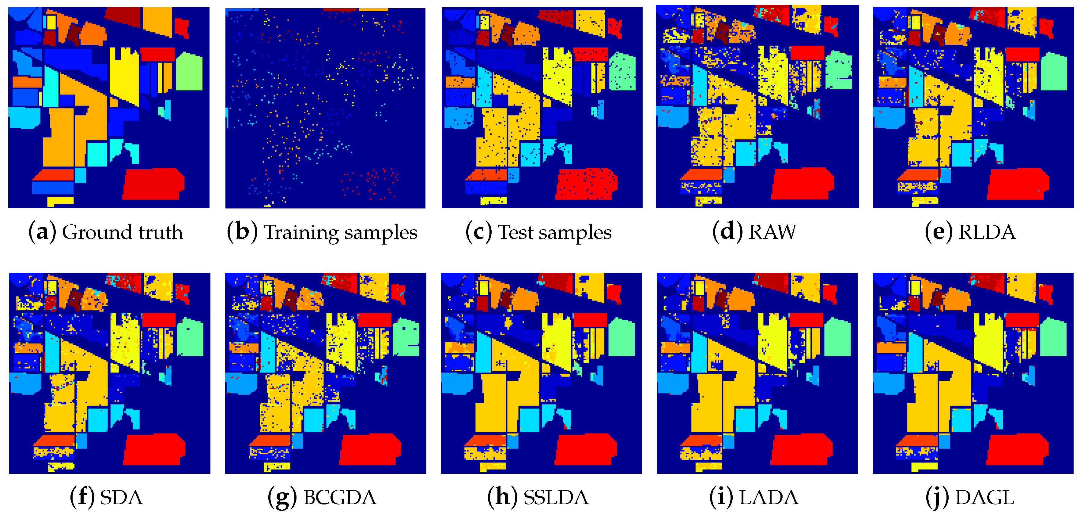
Furthermore, the classification maps of different methods on Indian Pines are also visualized in Figure 3. SSLDA, LADA and DAGL, which enforce the spatial smoothness within a small region, show better visualization quality than the others. Thus, the utilization of spatial information improves the classification performance. It is worth mentioning that the methods with spatial constraints are time-consuming, as shown in Table 3 and Table 4, since they need to find the surroundings and train the model for each sample. Compared to SSLDA and LADA, DAGL is more efficient because the optimization method converges fast.

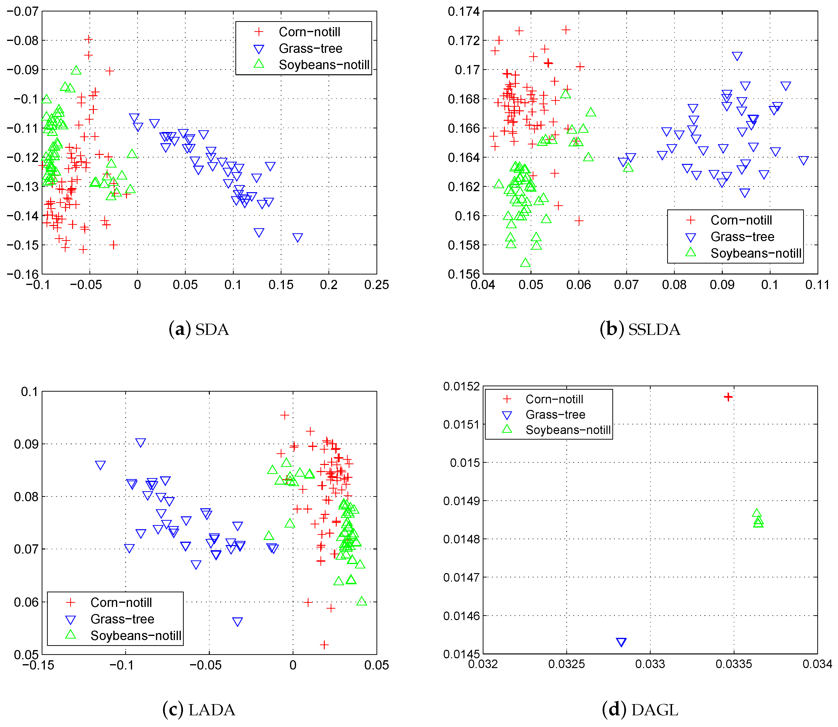
Similar to the experiments on toy dataset, we also visualize the two-dimensional subspace learned from the Indian Pines dataset. Taking the 5% samples from the Corn-notill, Grass-tree and Soybeans-notill classes, we project the data into two-dimensional subspace with SDA, SSLDA, LADA and the proposed DAGL. In this experiment, the spatial-smoothness terms of SSLDA, LADA and DAGL are removed so that we do not need to train the models for each sample separately. Figure 4 shows the projected data, the subspace found by DAGL separates the samples from different classes far away. This result explains the good performance of DAGL on the Indian Pines dataset when the reduced dimensionality is low.

4.3. Convergence and Parameter Sensitivity

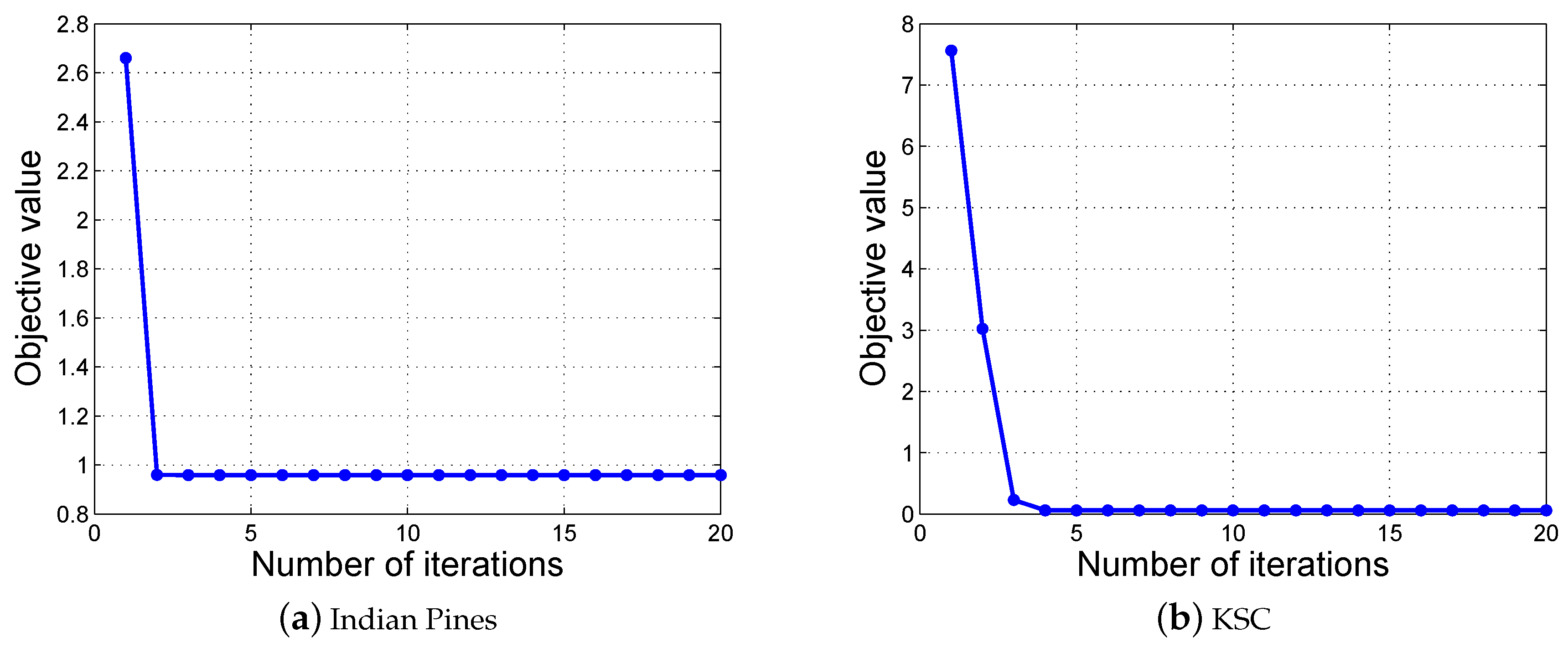
The convergence behavior of the proposed optimization algorithm is studied experimentally. We randomly choose two test samples from the Indian Pines and KSC datasets, and plot the changes of the objective values during the optimization. From Figure 5, we can see that the objective values of problem (11) converge within five iterations, which verifies that the optimization algorithm is effective and efficient.

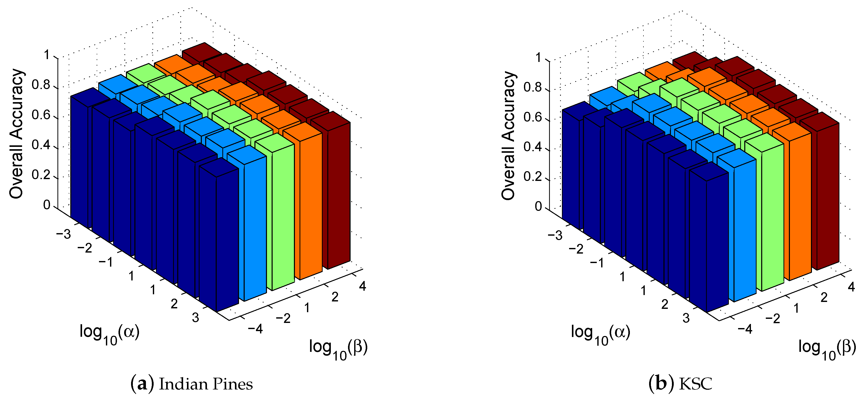
In addition, the parameter sensitivity of DAGL is also discussed. The objective function (11) contains two parameters, i.e., $\alpha$ and $\beta$. $\alpha$ affects the learning of the data graph, while $\beta$ controls the weight of the spatial smoothness term. With varying $\alpha$ and $\beta$, the variance of OA is shown in Figure 6. We can see that DAGL is robust to $\alpha$ and $\beta$ in a wide range. When $\alpha$ and $\beta$ become very small, the performance drops because the graph quality decreases and the spatial smoothness cannot be guaranteed.

5. Conclusions

In this paper, we propose a new supervised dimensionality reduction method, known as Discriminant Analysis with Graph Learning (DAGL). DAGL learns the data graph automatically during the discriminant analysis. It pulls the within-class similar samples together while pushing the between-class similar samples far away. Compared with LDA and its graph-based variants, DAGL is able to learn the data relationship within the desired subspace, which contains more valuable features and less noise. In addition, DAGL ensures the smoothness within the neighborhood, so it can discover the spatial correlation within hyperspectral images. Through the experiments on Indian Pines and KSC datasets, DAGL provides better classification results than the state-of-the-art competitors.

In future work, we would like to generalize the proposed method to the kernel version, and learn the nonlinear transformation of HSI data. It is also desirable to improve the optimization algorithm to increase the computation efficiency.

References

- Wang, Q.; Zhang, F.; Li, X. Optimal Clustering Framework for Hyperspectral Band Selection. IEEE Trans. Geosci. Remote Sens. 2018. [Google Scholar] [CrossRef]
- Mitra, P.; Murthy, C.; Pal, S. Unsupervised Feature Selection using Feature Similarity. IEEE Trans. Pattern Anal. Mach. Intell. 2002, 24, 301–312. [Google Scholar] [CrossRef]
- He, X.; Cai, D.; Niyogi, P. Laplacian Score for Feature Selection. In Proceedings of the 18th International Conference on Neural Information Processing Systems, Vancouver, BC, Canada, 5–8 December 2005; pp. 507–514. [Google Scholar]
- Nie, F.; Xu, D.; Li, X.; Xiang, S. Semisupervised Dimensionality Reduction and Classification through Virtual Label Regression. IEEE Trans. Syst. Man Cybern. 2011, 41, 675–685. [Google Scholar]
- Cheng, G.; Yang, C.; Yao, X.; Guo, L.; Han, J. When Deep Learning Meets Metric Learning: Remote Sensing Image Scene Classification via Learning Discriminative CNNs. IEEE Trans. Geosci. Remote Sens. 2018, 56, 2811–2821. [Google Scholar] [CrossRef]
- Liu, W.; Yang, X.; Tao, D.; Cheng, J.; Tang, Y. Multiview Dimension Reduction via Hessian Multiset Canonical Correlations. Inf. Fusion 2018, 41, 119–128. [Google Scholar] [CrossRef]
- Wang, Q.; Wan, J.; Yuan, Y. Locality Constraint Distance Metric Learning for Traffic Congestion Detection. Pattern Recognit. 2018, 75, 272–281. [Google Scholar] [CrossRef]
- Wang, Q.; Wan, J.; Yuan, Y. Deep Metric Learning for Crowdedness Regression. IEEE Trans. Circuits Syst. Video Technol. 2017. [Google Scholar] [CrossRef]
- Li, X.; Chen, M.; Wang, Q. Locality Adaptive Discriminant Analysis. In Proceedings of the International Joint Conference on Artificial Intelligence, Melbourne, Australia, 19–25 August 2017; pp. 2201–2207. [Google Scholar]
- Nie, F.; Xiang, S.; Zhang, C. Neighborhood MinMax Projections. In Proceedings of the International Joint Conference on Artificial Intelligence, Hyderabad, India, 6–12 January 2007; pp. 993–998. [Google Scholar]
- Fan, Zi.; Xu, Y.; Zhang, D. Local Linear Discriminant Analysis Framework using Sample Neighbors. IEEE Trans. Neural Netw. 2011, 22, 1119–1132. [Google Scholar] [CrossRef] [PubMed]
- Lu, J.; Plataniotis, K.; Venetsanopoulos, A. Regularization Studies of Linear Discriminant Analysis in Small Sample Size Scenarios with Application to Face Recognition. Pattern Recognit. Lett. 2005, 26, 181–191. [Google Scholar] [CrossRef]
- Wan, H.; Guo, G.; Wang, H.; Wei, X. A New Linear Discriminant Analysis Method to Address the Over-Reducing Problem. In Proceedings of the International Conference on Pattern Recognition and Machine Intelligence, Warsaw, Poland, 30 June–3 July 2015; pp. 65–72. [Google Scholar]
- Prasad, S.; Bruce, L.M. Limitations of Principal Component Analysis for Hyperspectral Target Recognition. IEEE Geosci. Remote Sens. Lett. 2008, 5, 625–629. [Google Scholar] [CrossRef]
- Fukunaga, K. Introduction to Statistical Pattern Recognition, 2nd ed.; Academy Press: San Francisco, CA, USA, 1972; pp. 2133–2143. [Google Scholar]
- Hyper-spectral Remote Sensing Scenes. Available online: http://www.ehu.es/ccwintco/index.php/Hyper-spectral_Remote_Sensing_Scenes (accessed on 31 July 2014).
- Dong, Y.; Du, B.; Zhang, L.; Zhang, L. Dimensionality Reduction and Classification of Hyperspectral Images using Ensemble Discriminative Local Metric Learning. IEEE Trans. Geosci. Remote Sens. 2017, 55, 2509–2524. [Google Scholar] [CrossRef]
- Bandos, T.V.; Bruzzone, L.; Camps-Valls, G. Classification of hyperspectral images with regularized linear discriminant analysis. IEEE Trans. Geosci. Remote Sens. 2009, 47, 862–873. [Google Scholar] [CrossRef]
- Kumar, N.; Agrawal, R.K. Two-Dimensional Exponential Discriminant Analysis for Small Sample Size in Face Recognition. IJAISC 2016, 5, 194–208. [Google Scholar] [CrossRef]
- Cai, D.; He, X.; Han, J. Semi-Supervised Discriminant Analysis. In Proceedings of the IEEE International Conference on Computer Vision, Rio de Janeiro, Brazil, 14–21 October 2007; pp. 1–7. [Google Scholar]
- Yuan, H.; Tang, Y.; Lu, Y.; Yang, L.; Luo, H. Spectral-Spatial Classification of Hyperspectral Image based on Discriminant Analysis. Int. J. Artif. Intell. Soft Comput. 2014, 7, 2035–2043. [Google Scholar] [CrossRef]
- Wang, Q.; Meng, Z.; Li, X. Locality Adaptive Discriminant Analysis for Spectral-Spatial Classification of Hyperspectral Images. IEEE Trans. Geosci. Remote Sens. Lett. 2017, 14, 2077–2081. [Google Scholar] [CrossRef]
- Bressan, M.; Vitria, J. Nonparametric Discriminant Analysis and Nearest Neighbor Classification. Pattern Recognit. Lett. 2003, 24, 2743–2749. [Google Scholar] [CrossRef]
- Cai, D.; He, X.; Zhou, K.; Han, J.; Bao, H. Locality Sensitive Discriminant Analysis. In Proceedings of the International Joint Conference on Artificial Intelligence, Hyderabad, India, 6–12 January 2007; pp. 708–713. [Google Scholar]
- Ly, N.H.; Du, Q.; Fowler, J.E. Collaborative Graph-Based Discriminant Analysis for Hyperspectral Imagery. IEEE J. Sel. Top. Appl. Earth Obs. Remote Sens. 2014, 7, 2688–2696. [Google Scholar] [CrossRef]
- Wu, T.; Zhou, Y.; Zhang, R.; Xiao, Y.; Nie, F. Self-Weighted Discriminative Feature Selection via Adaptive Redundancy Minimization. Neurocomputing 2018, 275, 2824–2830. [Google Scholar] [CrossRef]
- Luxburg, U. A Tutorial on Spectral Clustering. Stat. Comput. 2007, 17, 395–416. [Google Scholar] [CrossRef]
- Shi, J.; Malik, J. Normalized Cuts and Image Segmentation. IEEE Trans. Pattern Anal. Mach. Intell. 2000, 22, 888–905. [Google Scholar]
- Yao, X.; Han, J.; Zhang, D.; Nie, F. Revisiting Co-Saliency Detection: A Novel Approach Based on Two-Stage Multi-View Spectral Rotation Co-Clustering. IEEE Trans. Image Process. 2017, 26, 3196–3209. [Google Scholar] [CrossRef] [PubMed]
- Huang, J.; Nie, F.; Huang, H.; Ding, C. Robust Manifold Nonnegative Matrix Factorization. ACM Trans. Knowl. Discov. Data 2013, 8, 11:1–11:21. [Google Scholar] [CrossRef]
- Huang, J.; Nie, F.; Huang, H. A New Simplex Sparse Learning Model to Measure Data Similarity for Clustering. In Proceedings of the International Joint Conference on Artificial Intelligence, Buenos Aires, Argentina, 25–31 July 2015; pp. 3569–3575. [Google Scholar]
- Liu, W.; Zha, Z.; Wang, Y.; Lu, K.; Tao, D. p-Laplacian Regularized Sparse Coding for Human Activity Recognition. IEEE Trans. Ind. Electron. 2016, 63, 5120–5129. [Google Scholar] [CrossRef]
- Nie, F.; Zhu, W.; Li, X. Unsupervised Feature Selection with Structured Graph Optimization. In Proceedings of the AAAI Conference on Artificial Intelligence, Phoenix, AZ, USA, 12–17 February 2016; pp. 1302–1308. [Google Scholar]
- Li, X.; Chen, M.; Nie, F.; Wang, Q. A Multiview-Based Parameter Free Framework for Group Detection. In Proceedings of the AAAI Conference on Artificial Intelligence, San Francisco, CA, USA, 4–9 February 2017; pp. 4147–4153. [Google Scholar]
- Nie, F.; Wang, X.; Jordan, M.; Huang, H. The Constrained Laplacian Rank Algorithm for Graph-Based Clustering. In Proceedings of the AAAI Conference on Artificial Intelligence, Phoenix, AZ, USA, 12–17 February 2016; pp. 1969–1976. [Google Scholar]
- Zhang, R.; Nie, F.; Li, X. Self-weighted spectral clustering with parameter-free constraint. Neurocomputing 2017, 241, 164–170. [Google Scholar] [CrossRef]
- Nie, F.; Wang, H.; Huang, H.; Ding, C. Joint Schatten p-norm and ℓp-norm Robust Matrix Completion for Missing Value Recovery. Knowl. Inf. Syst. 2015, 42, 525–544. [Google Scholar] [CrossRef]
Figure 1.
(a) Projection directions found by RLDA and DAGL; (b) one-dimensional data projected by RLDA; (c) one-dimensional data projected by DAGL. For a better illustration, the projected data is plotted in the plane coordinate system, and the horizon coordinate of the projected data is set as zero.
Figure 2.
Overall Accuracy (OA) versus the reduced dimensionality of different methods on (a) Indian Pines and (b) KSC datasets.
Figure 3.
Classification maps for the Indian Pines dataset with different dimensionality reduction methods.
Figure 4.
Two-dimensional subspace found by (a) SDA, (b) SSLDA, (c) LADA and (d) DAGL on Indian Pines dataset.
Figure 5.
Converge curves of the proposed optimization algorithm on (a) Indian Pines and (b) KSC datasets.
Figure 6.
OA with varying and on (a) Indian Pines and (b) KSC datasets.