A Cloud Detection Method for Landsat 8 Images Based on PCANet

Abstract

Cloud detection for remote sensing images is often a necessary process, because cloud is widespread in optical remote sensing images and causes a lot of difficulty to many remote sensing activities, such as land cover monitoring, environmental monitoring and target recognizing. In this paper, a novel cloud detection method is proposed for multispectral remote sensing images from Landsat 8. Firstly, the color composite image of Bands 6, 3 and 2 is divided into superpixel sub-regions through Simple Linear Iterative Cluster (SLIC) method. Then, a two-step superpixel classification strategy is used to predict each superpixel as cloud or non-cloud. Thirdly, a fully connected Conditional Random Field (CRF) model is used to refine the cloud detection result, and accurate cloud borders are obtained. In the two-step superpixel classification strategy, the bright and thick cloud superpixels, as well as the obvious non-cloud superpixels, are firstly separated from potential cloud superpixels through a threshold function, which greatly speeds up the detection. The designed double-branch PCA Network (PCANet) architecture can extract the high-level information of cloud, then combined with a Support Vector Machine (SVM) classifier, the potential superpixels are correctly classified. Visual and quantitative comparison experiments are conducted on the Landsat 8 Cloud Cover Assessment (L8 CCA) dataset; the results indicate that our proposed method can accurately detect clouds under different conditions, which is more effective and robust than the compared state-of-the-art methods.

1. Introduction

With the development of remote sensing technology, remote sensing images are widely used in land cover monitoring, environmental monitoring, geographic mapping and target recognizing and other fields [1,2,3,4,5]. The Global Energy and Water Cycle Experiment (GEWEX) Cloud Assessment database estimates that the global annual average cloud cover is approximately 68% [6]. As a result, clouds will cause a lot of difficulty to target detection, object recognition and other tasks and ultimately cause incorrect analysis results [7,8]. Therefore, cloud detection is an important preprocessing step in various remote sensing applications.

Over the years, a number of cloud detection methods have been proposed for optical remote sensing images. In general, these methods can be mainly classified into two categories [9]: single-image-based methods and multiple-images-based methods. The multiple-images-based methods [10,11,12] require a set of images taken under the same grounds at different times. Hagolle et al. [13] developed a Multi-Temporal Cloud Detection (MTCD) method using time series of images from Formosat-2 and Landsat, and the results indicate that the MTCD method is more accurate than the Automatic Cloud Cover Assessment method. Chen et al. [14] proposed an iterative haze optimized transformation for automatic cloud/haze detection of Landsat image with the help of a corresponding clear image. Qian et al. [15] designed an automated cloud detection algorithm named Mean Shift Cloud Detection (MSCD) using multi-temporal Landsat 8 Operational Landsat Imager (OLI) data without any reference images. However, these methods need more images over a short time period to ensure that the ground surface underneath does not change much. In addition, a clear reference image is difficult to acquire.

Compared with multiple-images-based methods, cloud detection methods based on a single scene are more common and popular due to the reduced requirement for input data. Early single-image-based methods are mainly based on threshold [16,17,18], which extract various spectral features for each pixel, then use several thresholds to determine cloud pixels [19]. Cihlar and Howarth [20] used the Normalized Difference Vegetation Index (NDVI) to detect cloud pixels in AVHRR images. Irish [21] performed the Automated Cloud Cover Assessment (ACCA) system to screen clouds in Landsat data by applying a number of spectral filters, and depending heavily on the thermal infrared band. Zhu et al. [22,23] provided a cloud detection method for Landsat images by detecting potential cloud pixels combined with the cloud probability mask. Yang et al. [24] developed a progressive optimal scheme for detecting clouds in Landsat 8 image, which is based on the statistical properties and spectral properties derived from a large number of the images with cloud layers. The threshold-based cloud detection methods usually utilize only the low-level spectral information, and neglect the spatial information, which do not always work well for cloudy images under different imaging conditions because of its sensitivity to the underlying surface and the range of cloud cover [25,26].

Subsequently, more sophisticated methods have been developed [27,28,29]. Danda et al. [30] presented a morphology-based approach to coarsely detect clouds in remote sensing images based on a single band. As cloud and cloud shadow always occur in pairs, the relationship between cloud and cloud shadow as well as sun and satellite angles were used to improve the detection accuracy of cloud and cloud shadow [31]. An automatic multi-feature combined method for cloud and cloud shadow detection in GaoFen-1 wide field of view image was proposed by Li et al. [32], and acquired relatively satisfactory performance. In these methods, not only simple spectral information, but also other manually selected information of images was used for cloud detection, such as texture information, structure information, geometric information, and so on.

With the development of machine learning technology, machine-learning-based cloud detection methods [33,34] have attracted increasing study, which can extract more robust and high-level information from images. Hu et al. [35] adopted a visual attention technique in computer vision based on random forest to automatically identify images with a significant cloud cover. Li et al. [36] exploited the brightness and texture features to detect clouds based on SVM. An and Shi [37] proposed an automatic supervised remote-sensing image cloud detection approach based on the scene-learning scheme with two modules: feature data simulating and cloud detector learning and applying. In these machine-learning-based methods, a larger number of features were artificially designed and extracted as the input of classifier. These artificially designed features rely on prior knowledge and sensor, and they are difficult to accurately represent the characteristics of clouds with complex underlying surface.

Recently, deep learning methods have made significant progress in many computer visual tasks [38,39,40,41], and the cloud detection methods based on deep learning have attracted attention [42,43]. Shi et al. [44] and Goff et al. [45] used superpixel segmentation and deep Convolutional Neural Networks (CNNs) to detect clouds from Quickbird and Google Earth images and SPOT 6 images, respectively. Ozkan et al. [46] adapted a deep pyramid network to tackle cloud detection task, which can obtain accurate pixel-level segmentation and classification results from a set of noisy labeled RGB color remote sensing images. These methods achieved higher cloud detection accuracy than traditional machine learning methods.

In this paper, a novel cloud detection method is proposed for the multispectral remote sensing images with 9 bands from Landsat 8 OLI. The proposed method firstly obtains the coarse result by a spectral threshold function, then the accurate cloud detection result is obtained by a double-branch PCANet combined with SVM. The remainder of this paper is organized as follows. Section 2 presents the details of the proposed cloud detection method. Experimental results and analysis are described and discussed in Section 3. Finally, a conclusion is drawn in Section 4.

2. Methodology

Cloud is an aerosol comprising a visible mass of condensed droplets or frozen crystals suspended in the atmosphere. In the visible bands, the optical properties of water droplets and frozen crystals not only make clouds reflective, but also increase light absorption, thus reducing the transmittance of the radiation information from the underlying surface [47]. Intuitively, it seems that clouds are easily separable from ground objects, as clouds are generally white and bright compared to the underlying surface. Nevertheless, there are clouds that are not white or bright as well as bright ground objects, such as semitransparent thin clouds, bright buildings and snow, which are difficult to distinguish by spectral characteristics alone. Therefore, for high-accuracy cloud detection, both the spectral and spatial information of remote sensing image should be adequately considered.

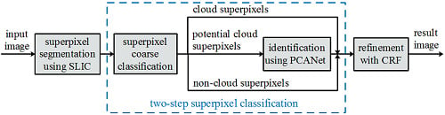
In this paper, a novel cloud detection method considering both spectral and spatial information is proposed for the multispectral remote sensing images, which is a combination of threshold-based method and machine-learning-based method. Figure 1 shows the flow chart of the proposed method. Firstly, the image is divided into spectrally homogeneous segments, namely superpixels, by SLIC [48] method. Then, a two-step classification strategy is used to divide these superpixels into cloud and non-cloud. The first step coarsely divides the superpixels into cloud, non-cloud and potential cloud by a spectral threshold function. The second step further classifies the potential cloud as cloud and non-cloud using the PCANet combined with SVM. Finally, a fully connected CRF [49] model is employed to refine the cloud detection result and accurate cloud borders are obtained.

Cloud detection methods based on sub-region can utilize the local spatial information of the image to avoid isolated point noise. Two deep-learning-based methods in [44,45] extracted features and predicted the class of each sub-region to detect clouds. It is time- consuming when use supervised learning methods to predict the class for all sub-regions. In addition, they learn features from all sub-regions including easy distinguished samples and hard distinguished samples, which increases the learning difficulty and causes low generalization ability.

In our framework, we pay more attention to hard samples through a two-step superpixel classification strategy. These hard samples are usually corresponding to bright ground objects and thin semitransparent clouds, which cannot be identified directly by spectral features. We use a threshold function to separate the obvious cloud and non-cloud superpixels from the ambiguous superpixels, thus improving cloud detection speed. Then, a double-branch PCANet is designed and combined with SVM to further predict the ambiguous superpixels as cloud or non-cloud. The inputs of the two branches of the designed PCANet are 9-dimensional Top of Atmosphere (TOA) reflectance data and 5-dimensional spectral feature data, respectively. The double-branch PCANet takes both spectral and spatial information into account. In addition, the classifier only needs to learn the features of the ambiguous superpixels without interference from the easy distinguished superpixels, which make the classification of the ambiguous superpixels become easier. Therefore, the combination of the two steps can obtain a more accurate cloud detection result.

2.1. Data and Preprocessing

The Landsat 8 OLI data is used to evaluate our method in this paper, which consists of 9 spectral bands with a spatial resolution of 30 m for Bands 1 to 7 and 9, and the resolution for Band 8 is 15 m. Band 1 is specifically designed for water resources and coastal zone investigation, and Band 9 is useful for cirrus cloud detection.

Table 1. Landsat 8 OLI spectral bands.

Band	Wavelength (Micrometers)	Resolution (Meters)
Band 1—Coastal	0.43–0.45	30
Band 2—Blue	0.45–0.51	30
Band 3—Green	0.53–0.59	30
Band 4—Red	0.64–0.67	30
Band 5—Near Infrared (NIR)	0.85–0.88	30
Band 6—Short Wavelength Infrared (SWIR) 1	1.57–1.65	30
Band 7—Short Wavelength Infrared (SWIR) 2	2.11–2.29	30
Band 8—Panchromatic	0.50–0.68	15
Band 9—Cirrus	1.36–1.38	30

shows the details of the 9 bands.

In the proposed method, the input data are TOA reflectances for Landsat 8 OLI bands. Standard Landsat 8 OLI data products consist of quantized and calibrated scaled Digital Numbers (DN) representing multispectral image data. To work on Landsat 8 OLI data, DN firstly need to be converted to TOA reflectance following equations described in [50].

$${\rho }_{{\lambda }^{\prime }}=M_{\rho }{Q}_{cal}+A_{\rho }$$

(1)

where ${\rho }_{{\lambda }^{\prime }}$ is TOA reflectance without correction for solar angle, $M_{\rho }$ is band-specific multiplicative rescaling factor, $Q_{cal}$ is quantized and calibrated standard product pixel values (DN), and $A_{\rho }$ is band-specific additive rescaling factor. TOA reflectance with a correction for the sun angle is then:

$${\rho }_{\lambda }=\frac{{\rho }_{{\lambda }^{\prime }}}{cos\left({\theta }_{SZ}\right)}=\frac{{\rho }_{{\lambda }^{\prime }}}{sin\left({\theta }_{SE}\right)}$$

(2)

where ${\rho }_{\lambda }$ is TOA reflectance with correction for solar angle, ${\rho }_{{\lambda }^{\prime }}$ is TOA reflectance without correction for solar angle, $cos\left({\theta }_{SZ}\right)$ is local solar zenith angle and $sin\left({\theta }_{SE}\right)$ is local sun elevation angle.

In addition, as the spatial resolution of Band 8 is 15 m, which is higher than other bands, we first resample it to 30 m spatial resolution for a uniform size.

2.2. Superpixel Segmentation

In [36], cloudy image was divided into sub-blocks of the same size according to the spatial position, then, the brightness and textural features were calculated to predict the class for each sub-block. However, the rigid division cannot be adaptive for the varied shape and size of clouds. In this paper, SLIC [48] is used to divide remote sensing image into superpixels, which are taken as the basic unit in the following procedures.

SLIC performs a local clustering of pixels and can efficiently generate compact and regular superpixels as sub-regions, which adhere well to the boundaries. According to [48], the clustering is applied in the labxy color-image plane space defined by the pixel’s CIELAB color space ${[l,a,b]}^{\mathrm{T}}$ and the pixel’s position ${[x,y]}^{\mathrm{T}}$. The distance measure between the pixel i and pixel j in the labxy space is defined as:

$$d_c=\sqrt{{(l_i-l_j)}^2+{(a_i-a_j)}^2+{(b_i-b_j)}^2}$$

(3)

$$d_s=\sqrt{{(x_i-x_j)}^2+{(y_i-y_j)}^2}$$

(4)

$$D_s=\sqrt{{\left(\frac{d_c}{m}\right)}^2+{\left(\frac{d_s}{S}\right)}^2}$$

(5)

where S is the square root of the required pixel number of the superpixel, m is the weight to control the importance between color similarity and spatial proximity. In this paper, m and S are set to 20 and 50, respectively.

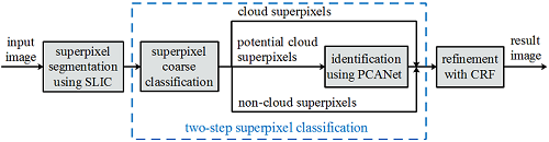
For Landsat 8 images, the Bands 6, 3 and 2 correspond to the short-wave infrared, green and blue bands, respectively. In their color composite image, the cloud is more obvious and easily distinguishable from snow/ice [51]. In this paper, SLIC method is executed on the color composite image using Bands 6, 3 and 2. Figure 2 is an example of superpixel segmentation, where (a) is the color composite image of Bands 6, 3 and 2, (b) is the superpixel segmentation result of (a). It can be seen that the cloud superpixels adhere well to cloud boundaries. In this paper, we adopt a two-step classification strategy to recognize each superpixel as cloud or non-cloud.

2.3. Superpixel Coarse Classification

It can be seen from Figure 2b that there are three kinds of superpixels in the image: (1) bright and thick cloud superpixels, (2) obvious non-cloud superpixels, (3) potential cloud superpixels, including dark cloud, semi-transparent thin cloud and bright non-cloud. The first two kinds of superpixels are easily recognized, and we use a brightness feature combined with the threshold method to separate them from the potential cloud superpixels, which can simplify the calculation and improve detection speed.

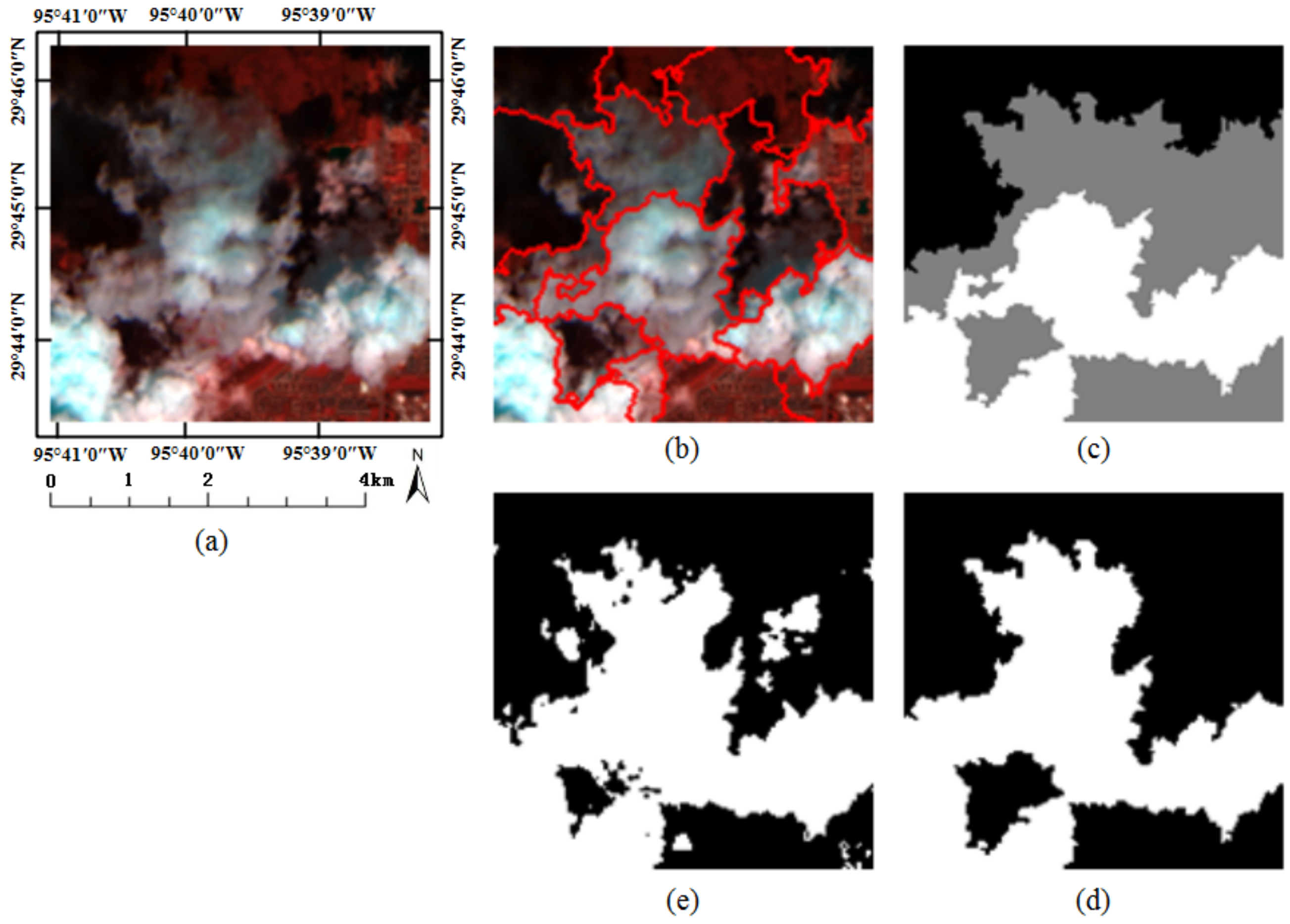
Clouds on the remote sensing images are mainly uniform flat, and a large proportion of them are brighter than most of the Earth’s surface [9,36]. We define a brightness feature to enhance the difference between cloud pixels and non-cloud pixels:

$$b=\frac{1}{3}{\sum }_{i\in 2,3,6}\mathrm{Band}i\times \frac{{min}_{i\in 2,3,6}\mathrm{Band}i}{{max}_{i\in 2,3,6}\mathrm{Band}i}$$

(6)

where Band i is the TOA reflectance of the i-th band, which is normalized to [0, 1].

For a cloud pixel, the TOA reflectance values are large and close to each other in Bands 6, 3 and 2, and therefore the value of b is big. While for a non-cloud pixel, the TOA reflectance values are varied in the three bands, and the average TOA reflectance value is small, and therefore the value of b is small.

Then, we calculate the brightness feature for each pixel. We selected 24 images from L8 CCA dataset [51] (Landsat ID and Cloud Cover of the 24 images are given in

Table A1. Landsat ID and Cloud Cover of the 24 training images.

Biome	Landsat ID	Cloud Cover
	LC80420082013220LGN00	0.00%
Barren	LC81550082014263LGN00	100.00%
	LC81990402014267LGN00	85.64%
	LC80500172014247LGN00	65.83%
Forest	LC81310182013108LGN01	5.44%
	LC82310592014139LGN00	99.68%
	LC81320352013243LGN00	32.41%
Grass/Crops	LC81440462014250LGN00	100.00%
	LC81490432014141LGN00	0.12%
	LC80670172014206LGN00	92.81%
Shrubland	LC80750172013163LGN00	0.12%
	LC80760182013170LGN00	52.91%
	LC80250022014232LGN00	79.49%
Snow/Ice	LC81321192014054LGN00	20.01%
	LC82171112014297LGN00	54.47%
Urban	LC81620432014072LGN00	20.29%
	LC81940222013245LGN00	100.00%
	LC80650182013237LGN00	51.32%
Water	LC81660032014196LGN00	95.24%
	LC81910182013240LGN00	0.42%
	LC81070152013260LGN00	100.00%
Wetlands	LC81080182014238LGN00	53.07%
	LC81460162014168LGN00	0.00%

), and calculated the cumulative probability distribution of b for cloud pixels and non-cloud pixels, respectively, as shown in Figure 3. The red line is the cumulative probability curve of non-cloud pixel, and the blue line is that of cloud pixel. It can be observed that about 98% of the non-cloud pixels have a b value less than 0.176, and about 98% of the cloud pixels have a b value greater than 0.073.

Therefore, for a superpixel, we define a threshold function as follows:

$$T\left({\Omega }\right)=\frac{{\displaystyle \sum _{z\in {\Omega }}}\psi \left(z\right)}{N\left({\Omega }\right)}$$

(7)

$$\psi \left(z\right)=\left\{\begin{array}{cc}\hfill -1,& \hfill b\left(z\right)<0.073\\ \hfill 0,& \hfill 0.073\le b\left(z\right)\le 0.176\\ \hfill 1,& \hfill b\left(z\right)>0.176\end{array}\right.$$

(8)

where $N\left({\Omega }\right)$ is the number of pixels in the superpixel ${\Omega }$, and $b\left(z\right)$ is the brightness feature b of pixel z.

If $T\left({\Omega }\right)<-0.7$, the superpixel ${\Omega }$ is predicted as non-cloud, and if $T\left({\Omega }\right)>0.7$, the superpixel ${\Omega }$ is predicted as cloud, and otherwise, it is potential cloud. Figure 2c shows the superpixel coarse classification result of Figure 2b, where white represents the cloud superpixels, black represents the non-cloud superpixels and gray represents the potential cloud superpixels.

2.4. Identification of the Potential Cloud Superpixels

The potential cloud superpixels generally contain high brightness ground objects and thin semitransparent clouds, which are difficult to be identified by the low-level spectral information. We use PCANet to extract the high-level features of clouds, which are fed to a linear SVM classifier to obtain a better classification result.

2.4.1. A Brief Introduction to PCANet

PCANet is a simple deep learning network for image classification [52,53]. Compared with CNN, the most important change in PCANet is that the data-adapting convolution filter bank in each stage is replaced by basic PCA filter, and the nonlinear layer adopting the simplest binary quantization (hashing), and for the feature pooling layer, the block-wise histograms of the binary codes are employed, which are the final extracted features of the network. PCANet is easy to be trained and adapted to different data and tasks, and can avoid the problem of parameter training in traditional CNN that consumes too much time and requires various ad hoc tricks [54,55].

PCANet is a cascaded network, which is based on three basic data processing components: cascaded principal component analysis (PCA), binary hashing, and block-wise histograms. Suppose that there are N training images ${\left\{{\mathbf{I}}_i\right\}}_{i=1}^N$ of size $w\times h$, and the filter size is $k_1\times k_2$ at all stages. For the i-th training image ${\mathbf{I}}_i$, PCANet takes a $k_1\times k_2$ patch around each pixel, and collects all the vectorized mean-removed patches to form a matrix ${\overline{\mathbf{X}}}_i\in {\mathbb{R}}^{\left(k_1{k}_2\right)\times n}$, where n is the number of patches extracted from ${\mathbf{I}}_i$. By constructing the same matrix for all training images and combining them, we obtain

$$\mathbf{X}=[{\overline{\mathbf{X}}}_1,{\overline{\mathbf{X}}}_2,\cdots ,{\overline{\mathbf{X}}}_N]\in {\mathbb{R}}^{\left(k_1{k}_2\right)\times \left(Nn\right)}$$

(9)

Assuming that the number of filters in the first layer is $L_1$. PCA minimizes the reconstruction error within a family of orthonormal filters, i.e.,

$$\underset{\mathbf{V}\in {\mathbb{R}}^{\left(k_1{k}_2\right)\times L_1}}{min}{∥\mathbf{X}-\mathbf{V}{\mathbf{V}}^{\mathrm{T}}\mathbf{X}∥}_F^2,s.t.{\mathbf{V}}^{\mathrm{T}}\mathbf{V}={\mathbf{E}}_{L_1}$$

(10)

where ${\mathbf{E}}_{L_1}$ is an identity matrix with size $L_1\times L_1$. The solution is the $L_1$ principal eigenvectors of $\mathbf{X}{\mathbf{X}}^{\mathrm{T}}$. Therefore, the PCA filters can be expressed as

$${\mathbf{W}}_l^1\stackrel{.}{=}\mathrm{ma}{\mathrm{t}}_{\left(k_1{k}_2\right)}\left({\mathbf{q}}_l\left(\mathbf{X}{\mathbf{X}}^{\mathrm{T}}\right)\right)\in {\mathbb{R}}^{k_1\times k_2},l=1,2,\cdots ,L_1$$

(11)

where ${\mathrm{mat}}_{\left(k_1{k}_2\right)}\left(\mathbf{v}\right)$ is a function that reshapes a vector $\mathbf{v}\in {\mathbb{R}}^{k_1{k}_2}$ to a matrix $\mathbf{W}\in {\mathbb{R}}^{k_1\times k_2}$, and ${\mathbf{q}}_l\left(\mathbf{X}{\mathbf{X}}^{\mathrm{T}}\right)$ denotes the l-th principal eigenvector of $\mathbf{X}{\mathbf{X}}^{\mathrm{T}}$. Then, the l-th filter output of the first layer can be obtained by

$${\mathbf{I}}_i^l\stackrel{.}{=}{\mathbf{I}}_i\ast {\mathbf{W}}_l^1,i=1,2,\cdots ,N$$

(12)

where * denotes 2D convolution. For each input image ${\mathbf{I}}_i$, the first layer will output $L_1$ images. Executing the same process as in the first layer for all the obtained ${\mathbf{I}}_i^l$, the output of the second layer is obtained. Assuming that the number of filters in the second layer is $L_2$, PCANet would output $L_1{L}_2$ images for each input image. A deeper PCANet architecture can be built by repeating the above process, to extract higher level features. Two layers are enough for most tasks according to [52].

After the process of PCA filter, a binary hashing process is followed. This process binarizes $L_2$ outputs and converts them into a single integer-valued “image”. Subsequently, each of the $L_1$ images is divided into many local blocks. Then, computing the histogram of each block (with $2^{L_2}$ bins), and concatenating all the histograms into one vector, which is the feature expression for input image ${\mathbf{I}}_i$. Finally, the classification result is determined by a linear SVM classifier.

2.4.2. Our Designed Double-Branch PCANet

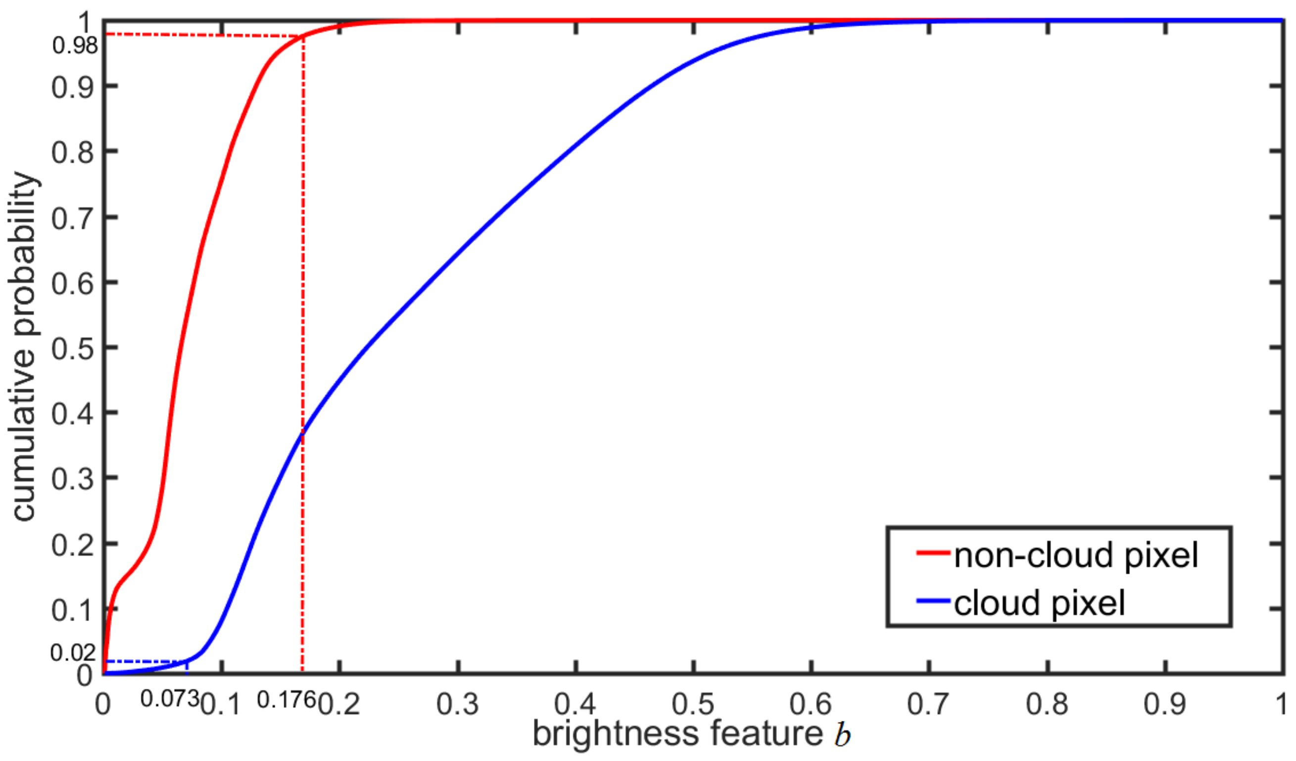
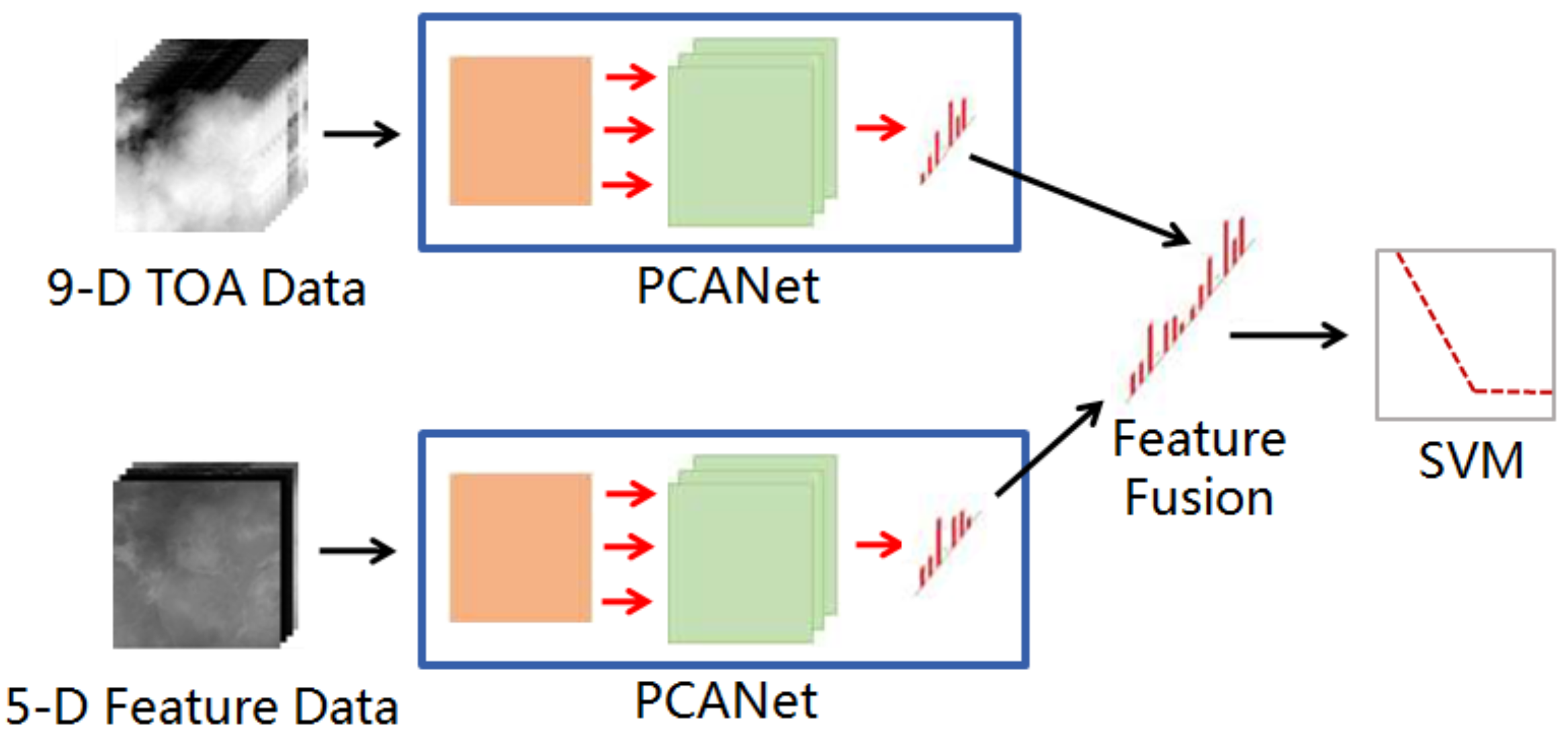
In this paper, a double-branch PCANet is designed, as shown in Figure 4. The input of the first branch is the 9-dimensional TOA reflectance data (Band 1–Band 9), which fuses the spectral information of nine bands. In addition, the input of the second branch is five spectral feature maps including Normalized Difference Snow Index (NDSI), NDVI, B5/B6, “Whiteness”, and Haze Optimized Transformation (HOT), which are defined as:

$$\mathrm{NDSI}=\left(\mathrm{Band}3-\mathrm{Band}6\right)/\left(\mathrm{Band}3+\mathrm{Band}6\right)$$

(13)

$$\mathrm{NDVI}=\left(\mathrm{Band}5-\mathrm{Band}4\right)/\left(\mathrm{Band}5+\mathrm{Band}4\right)$$

(14)

$$\begin{array}{cc}\hfill \mathrm{meanVis}& =\left(\mathrm{Band}2+\mathrm{Band}3+\mathrm{Band}4\right)/3,\hfill \\ \hfill \mathrm{Whiteness}& =\sum _{i=2}^4\left|(\mathrm{Band}i-\mathrm{meanVis})/\mathrm{meanVis}\right|\hfill \end{array}$$

(15)

$$\mathrm{HOT}=\mathrm{Band}2-0.5\times \mathrm{Band}4-0.08$$

(16)

$$\mathrm{B}5/\mathrm{B}6=\mathrm{Band}5/\mathrm{Band}6$$

(17)

In [21], Irish used NDSI, NDVI and B5/B6 indexes to separate clouds from the snow, vegetation and bright rocks, respectively. “Whiteness” index was employed by Gomez-Chova et al. [56] to exclude pixels that are not white enough to be clouds. The HOT index was firstly proposed by Zhang et al. [57], which has been widely used for haze reduction and cloud detection. Zhu et al. [22] identified the potential cloud pixels by combining five spectral feature maps. In this paper, we use the five spectral feature maps to describe the features of the potential cloud pixels. The two branches of the designed PCANet are used to retrieve the high-level features from 9-dimensional TOA reflectance data and 5-dimensional spectral feature data, respectively. Finally, these high-level features are fused and fed to a linear SVM classifier to obtain the final classification result. Figure 2d shows the two-step superpixel classification result of Figure 2b.

2.5. Refinement with Fully Connected CRFs

Through Section 2.3 and Section 2.4, each superpixel is classified as cloud or non-cloud, and the cloud detection result is based on superpixel. However, the regions around the boundaries of the clouds are usually thin semitransparent clouds, which will contain non-cloud pixels sometimes, and thus leading to wrong classification result. In [24,32,58], a guided filter was implemented to refine the detected cloud boundaries. It only utilizes the local spatial information and the binary cloud detection result, which ignores the global spatial information and the cloud probability of each pixel. In this paper, a global optimization strategy with fully connected CRF model [49] is applied to capture the thin clouds around cloud boundaries, then a more accurate refined cloud detection result is obtained.

The model employs the energy function [59]:

$$E\left(\mathbf{x}\right)=\sum _i{\theta }_i\left(x_i\right)+\sum _{ij}{\theta }_{ij}(x_i,x_j)$$

(18)

where $\mathbf{x}$ is the label of pixels, and $x_i$ and $x_j$ denote the labels of pixels i and j, respectively.

The first term in Equation (18) is a unary potential: ${\theta }_i\left(x_i\right)=-logP\left(x_i\right)$, where $P\left(x_i\right)$ is the cloud probability of pixel i. In Section 2.3, the superpixels are divided into three classes: cloud, non-cloud and potential cloud. The cloud probabilities of the pixels in cloud superpixel are set to 1, and those of the pixels in non-cloud superpixel are set to 0. For the pixels in the potential cloud superpixel, their cloud probabilities are obtained using the output of SVM in Section 2.4, which are normalized to [0, 1].

The second term in Equation (18) is a pairwise potential, which is the combination of two Gaussian kernels in terms of the colors and positions for pixels i and j:

$${\theta }_{ij}(x_i,x_j)=\mu (x_i,x_j)\left[{\omega }_{1}exp\left(-\frac{\Vert p_i-p_j{\Vert }^2}{2{\sigma }_{\alpha }^2}-\frac{\Vert c_i-c_j{\Vert }^2}{2{\sigma }_{\beta }^2}\right)+{\omega }_{2}exp\left(-\frac{\Vert p_i-p_j{\Vert }^2}{2{\sigma }_{\gamma }^2}\right)\right]$$

(19)

where $\mu (x_i,x_j)$ is a binary function, which is 0 when pixel i has the same label with pixel j, otherwise 1. $p_i$ and $c_i$ are the position and color vector (including Bands 6, 3 and 2 in this paper) of pixel i. The first bilateral kernel depends on both pixel position and color, which forces nearby pixels with similar color to have the same labels, and the second kernel only depends on pixel position, which only considers spatial proximity when enforcing smoothness. The parameters ${\omega }_1$ and ${\omega }_2$ are linear combination weights of the two Gaussian kernels, and ${\sigma }_{\alpha }$, ${\sigma }_{\beta }$ and ${\sigma }_{\gamma }$ control the scale of Gaussian kernels.

Minimizing the CRF energy function $E\left(\mathbf{x}\right)$ in Equation (18) yields the most probable label assignment $\mathbf{x}$ for the given image. Since this strict minimization is intractable, a mean field approximation to the CRF distribution $d\left(\mathbf{x}\right)={\prod }_i{d}_i\left(x_i\right)$ is used for approximate maximum posterior marginal inference. Figure 2e shows the fully connected CRF refinement result of Figure 2d.

3. Results and Discussion

In this paper, a cloud detection framework is proposed for multispectral remote sensing images, which is implemented in MATLAB release 2016a on a computer with Intel CPU i7-6700K at 4.00 GHz and 32.00 GB RAM.

The experimental images are from the L8 CCA dataset [51], which contains totally 96 images and their ground truth, the image effective size is approximately 6400 × 6400. In these experimental images, there are eight biomes including Barren, Forest, Grass/Cropland, Shrubland, Snow/Ice, Urban, Water, and Wetlands, and each biome has 12 scenes. These images are divided to two parts: 24 images (three for each biome) for training and the remaining 72 ones for test. The 24 training images are also used to determine the threshold in Section 2.3 when coarsely classifying the superpixels.

We used four metrics to quantitatively evaluate the performance of the methods, including the Right Rate (RR), Error Rate (ER), False Alarm Rate (FAR), and ratio of RR to ER (RER). They are defined as:

$$RR=\frac{CC}{TC}$$

(20)

$$ER=\frac{CN+NC}{TP}$$

(21)

$$FAR=\frac{NC}{TC}$$

(22)

$$RER=\frac{RR}{ER}$$

(23)

where CC denotes the number of cloud pixels detected as cloud pixels, TC denotes the total number of cloud pixels in ground truth, CN denotes the number of cloud pixels detected as non-cloud pixels, NC denotes the number of non-cloud pixels detected as cloud pixels, and TP denotes the total number of pixels in the input image.

According to the definition, it is obvious that RR represents the information of correctly detected clouds, ER provides us the information about the errors, and FAR indicates the information of incorrectly detected clouds. Using only one of them to evaluate algorithms is insufficient, as some methods may obtain high RR but also high ER. On the contrary, some methods may obtain low FAR but also low RR. Therefore, RER is defined to obtain an integrated result as it considers the RR and ER. A higher value of RER denotes better cloud detection result.

3.1. Training and Detection

For the proposed cloud detection framework, as shown in Figure 1, we need to train the PCANet combined with a linear SVM classifier, and determine the optimal parameters of the fully connected CRF model.

In the training stage, for the 24 training images, the superpixels are extracted using the SLIC method. Through superpixel coarse classification, 140,000 potential cloud superpixels are obtained. From the 140,000 superpixels (their ground truth are known), we randomly extract 35,000 cloud patches as positive samples, and 35,000 non-cloud patches as negative samples, and the patch size is 55 × 55. All the 70,000 samples are used to train the designed double-branch PCANet, which parameters setting is: two layers, 7 × 7 patch size, eight filters in each layer, 7 × 7 size of block histograms (non-overlapping).

In the refinement post-processing stage, we use default values of ${\omega }_2=1$ and ${\sigma }_{\gamma }=1$, and search for the best values of ${\omega }_1$, ${\sigma }_{\alpha }$ and ${\sigma }_{\beta }$ by cross-validation on the training set, and the final values of ${\omega }_1$, ${\sigma }_{\alpha }$ and ${\sigma }_{\beta }$ are 10, 300 and 3, respectively. We employ 20 mean field iterations in this paper.

In the detection stage, superpixels are first obtained from the test image using the SLIC method. Then, we calculate the brightness feature of the superpixels, and divide them into cloud, non-cloud and potential cloud by the spectral threshold function. For each potential superpixel, an image patch (55 × 55) centered at its geometric center pixel is extracted and inputted into the trained PCANet model, and thus, the class of the potential superpixel is predicted. Merging the classification results of all superpixels in the test image, the superpixel-based cloud detection result is obtained. Finally, a fully connected CRF model is employed to refine the cloud detection result and accurate cloud borders are obtained.

3.2. Effectiveness of Designed PCANet Architecture

Compared with the traditional CNNs, PCANet is simpler and faster. In this paper, a double-branch PCANet architecture is designed to extract the features of the potential clouds, and using these features, a linear SVM classifier is trained to classify the potential clouds.

In order to verify the effectiveness of the designed double-branch PCANet architecture, We compare our PCANet architecture with three CNN architectures, including AlexNet [38], VGG-16 [39] and ResNet-20 [40], and two single-branch PCANet (see the two branches of Figure 4). For the three compared CNNs, their inputs are the 9-dimensional TOA reflectance data. Since this experiment is to verify the performance of different network architectures, it does not include the superpixel coarse classification and the CRF refinement process. We extract 80,000 cloud patches and 320,000 non-cloud patches from 24 training images as training set for AlexNet, VGG-16 and ResNet-20, and the patch size is 55 × 55. Considering PCANet does not need a large training set, we extract 35,000 cloud patches and 35,000 non-cloud patches for training.

Table 2. Statistical results of different network architectures.

Methods	RR	ER	FAR	RER
AlexNet [38]	0.8966	0.0955	0.0986	9.3848
VGG-16 [39]	0.8919	0.0903	0.0829	9.8719
ResNet-20 [40]	0.9023	0.0865	0.0853	10.4252
single-branch PCANet (9-D)	0.9023	0.0829	0.0775	10.8854
single-branch PCANet (5-D)	0.8010	0.1164	0.0470	6.8828
double-branch PCANet	0.9138	0.0729	0.0680	12.5289

shows the statistical results of different network architectures on the test set. It can be seen that, compared with the three CNNs, the 9-dimensional single-branch PCANet has the best values in metrics ER, FAR and RER, in addition, its RR, the same as that of ResNet-20, is also the best. Therefore, the 9-dimensional single-branch PCANet outperforms the three compared CNNs. In two single-branch PCANets, the 5-dimensional PCANet has lower performance than the 9-dimensional one due to the incomplete spectral information input. In addition, when combining the two single-branch PCANets together, it is exactly our final double-branch PCANet, which obtains a better cloud detection result than both of the two single-branch PCANets. Overall, with the highest RR and RER and the lowest ER, our double-branch PCANet outperforms the five compared network architectures.

3.3. Effectiveness of the Proposed Cloud Detection Framework

A cloud detection framework is proposed in this paper. Firstly, we separate the obvious cloud and non-cloud superpixels from the potential cloud superpixels by superpixel coarse classification. Then, the designed double-branch PCANet is used to identify the potential cloud superpixels. Finally, the fully connected CRF is used to refine the cloud detection result, and we obtain the final finer result. In order to evaluate the effectiveness of the proposed framework, we compare it with three other frameworks, including the simple double-branch PCANet (without superpixel coarse classification and refinement process), the two-step superpixel classification strategy (superpixels coarse classification combined with double-branch PCANet, and without refinement process), and the two-step superpixel classification strategy combined with guided filter based refinement process. Here, the simple double-branch PCANet is exactly the double-branch PCANet used in Section 3.2, and the other two compared frameworks have the same training stage with our final cloud detection framework.

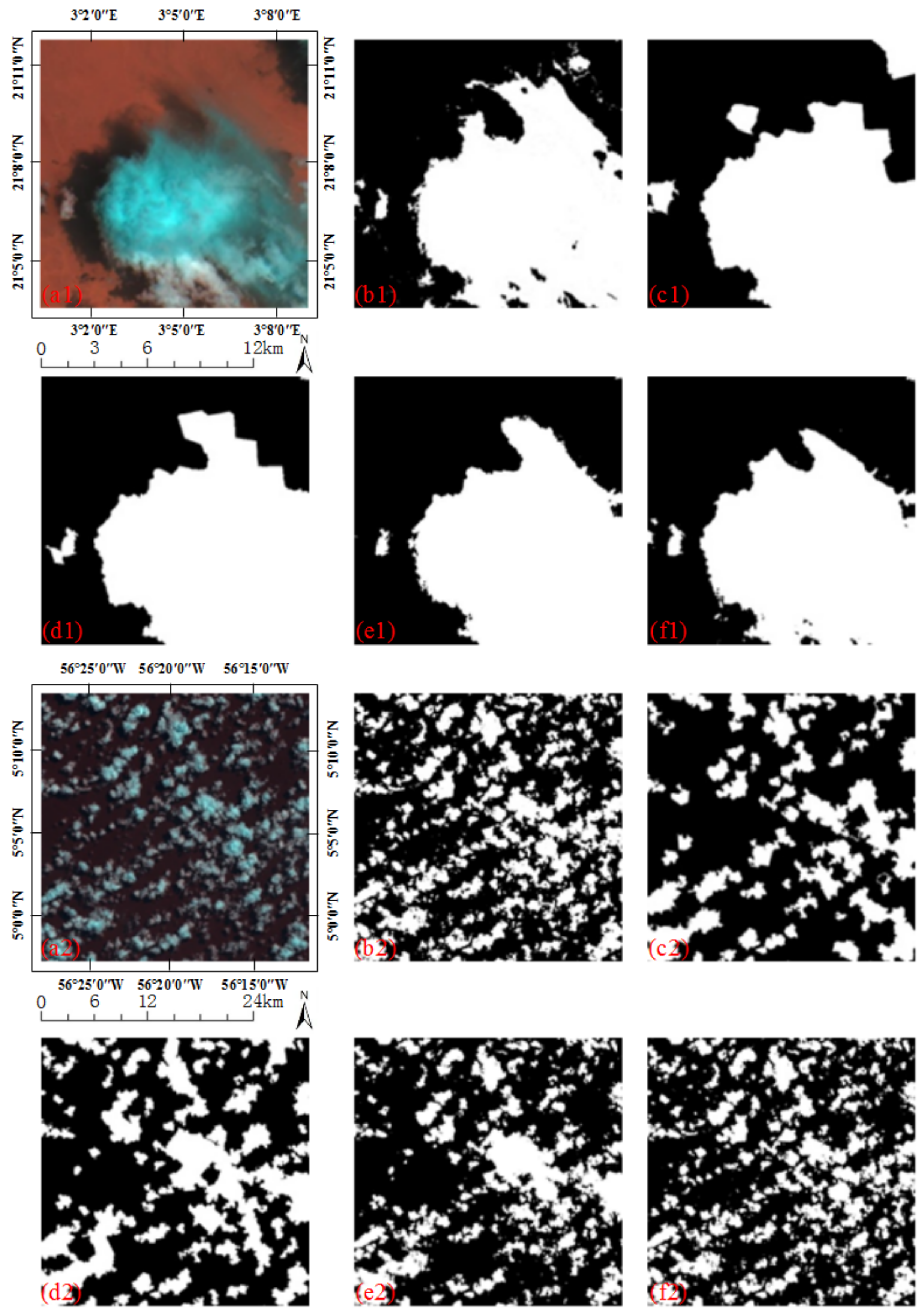
Figure 5 shows two instances of cloud detection, where (a1,a2) are the cloudy images composited of Bands 6, 3 and 2, (b1,b2) are ground truth and the white is cloud region, from (c1,c2) to (f1,f2) are the results of three compared method and our proposed final framework. It can be seen that the cloud in (a1) of Figure 5 is thick and clumpy, and the boundaries of the cloud detected by the first two compared methods are unsmooth and with blocking effect, because the first two compared methods are based on superpixel sub-region. While the last two methods (two-step strategy combined with guided filter and our method) use guided filter and CRF to correct the misclassified pixels, respectively, which are based on pixel, therefore the results have more accurate cloud boundary. The cloud is fractional in (a2) of Figure 5. When a superpixel contains non-cloud region much more than thin and small cloud region, it will probably be classified as non-cloud, and the cloud pixels in it are incorrectly detected. Conversely, when a superpixel contains cloud region much more than non-cloud region, it will probably be classified as cloud, and the non-cloud pixels in it are false detected. Therefore, the first two compared superpixel-based methods will cause missed detection and false detection, see (c2,d2) in Figure 5. When combining the two-step strategy with guided filter, the missed and false detected pixels around the boundaries of the cloud regions are corrected. Because guided filter only considers local information, the misclassified pixels are still obvious. Our method uses the global optimal CRF model to refine the cloud detection result, and a more accurate result is obtained.

Table 3. Statistical results of different cloud detection frameworks.

Methods	RR	ER	FAR	RER	Test Time
double-branch PCANet	0.9138	0.0729	0.0680	12.5289	19.3 min
two-step superpixel classification strategy	0.9194	0.0710	0.0695	12.9539	10.1 min
two-step strategy combined with guided filter	0.9192	0.0679	0.0628	13.5361	19.3 min
our proposed final framework	0.9338	0.0515	0.0426	18.1315	12.8 min

shows the statistical results of three compared cloud detection frameworks and the proposed framework on the test set. The last column in Table 3 shows the average detection time of each image. In the two-step superpixel classification, the first-step threshold method separates the easily distinguished superpixels from the potential cloud superpixels firstly, and the second-step PCANet pays more attention to the potential cloud superpixels. It can be seen that the two-step superpixel classification has a better cloud detection result than the simple double-branch PCANet, and its time cost is only 52.3% of the latter. Guided filter improves slightly the detection accuracy of the two-step superpixel classification, but its time cost increased greatly. While our proposed framework uses CRF to correct the misclassified pixels, the accuracy is obviously improved. In addition, our proposed framework only takes 26.7% more time than the two-step superpixel classification, but it still saves 33.7% of the time compared to the simple double-branch PCANet. Considering that it yields the best detection result, our final framework outperforms the other three methods.

3.4. Comparison with Other Cloud Detection Methods

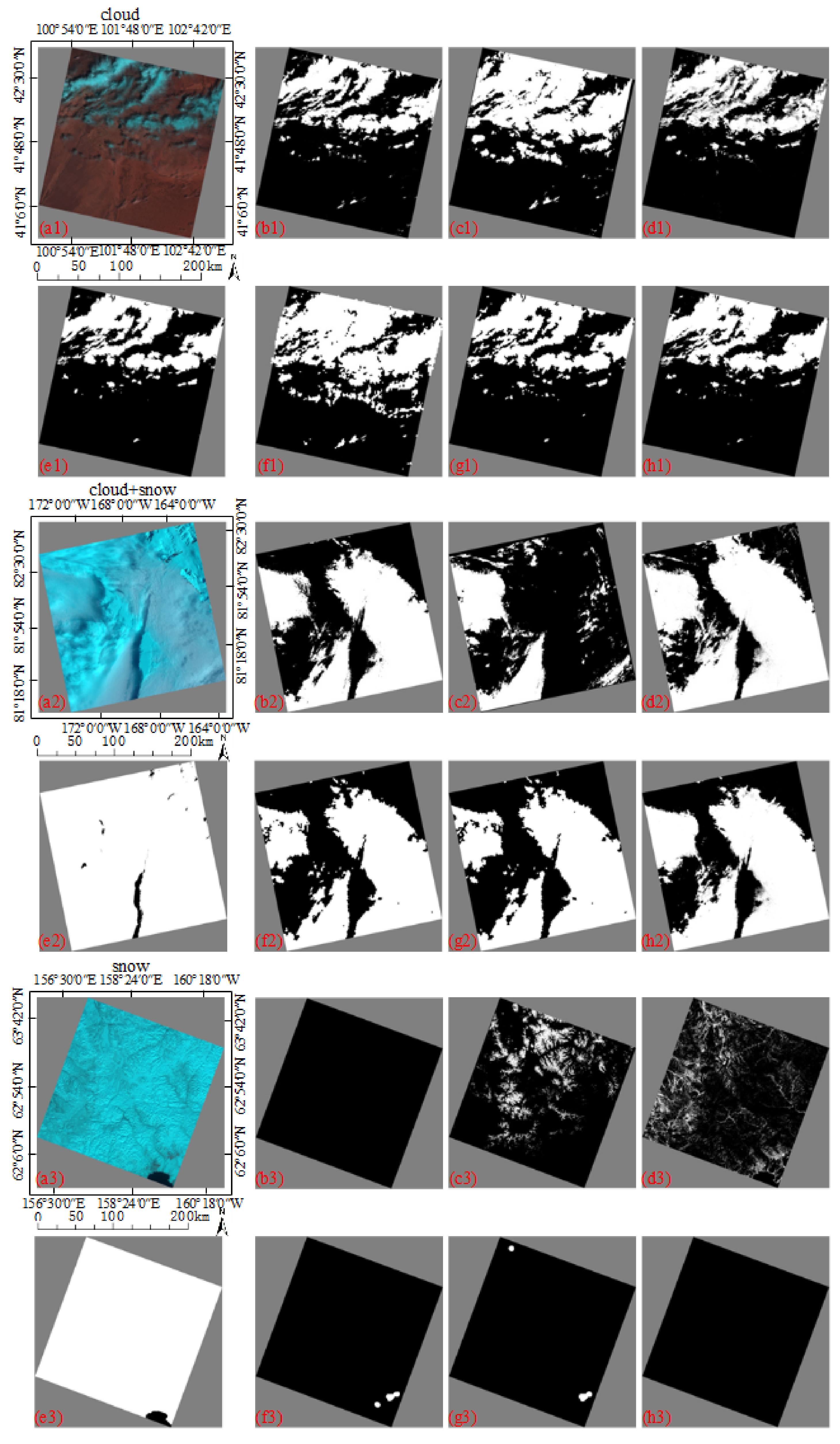
We compare our method with five other cloud detection methods including Zhu’s method [23], Yang’s method [24], Li’s method [32], Shi’s method [44] and Goff’s method [45], where the first three methods are unsupervised, and the last two methods are based on deep learning. In addition, Zhu’s method was an implementation from Fmask 3.2 version (download from http://ftp-earth.bu.edu/public/zhuzhe/Fmask_Windows_3.2v/), Shi’s method was implemented by Shi et al. (download from http://xfy.buaa.edu.cn/), and we reproduced Yang’s method, Li’s method and Goff’s method with default values. Figure 6 shows several cloud detection instances, where (a1–a3) are the original color composite images, (b1–b3) are ground truth and the white is cloud region, (c1–c3)–(h1–h3) are the results of five compared methods and our method. In Figure 6, the second image (a2) contains both cloud and snow, which are easily confused with each other, and the last image (a3) only has snow, without cloud. It can be observed that, for the three unsupervised methods, Li’s method is completely failed for the second and the third images and the snow pixels are misidentified as cloud, Zhu’s method misses many cloud pixels for the second image and falsely detects the snow pixels as cloud for the last image; Yang’s result is better than Li’s and Zhu’s results, but its false detection is obvious for the last image. For the two deep-learning-based methods, Shi’s method causes obviously false detection in the first image, Goff’s method has a similar cloud detection result with our method, but the former causes slight false detection in the last image. Overall, our cloud detection result is the best among the six methods.

Table 4. Statistical results of different cloud detection methods.

Methods	RR	ER	FAR	RER
Zhu’s method [23]	0.8714	0.1562	0.2017	5.5781
Yang’s method [24]	0.8935	0.1073	0.1203	8.3271
Li’s method [32]	0.9588	0.1586	0.2941	6.0466
Shi’s method [44]	0.8992	0.1013	0.1134	8.8789
Goff’s method [45]	0.8813	0.1096	0.1131	8.0381
Proposed method	0.9338>	0.0515	0.0426	18.1315

is the statistical results of different methods on the test set. It can be observed that Li’s method has the best RR, but its ER and FAR are rather high, which means there are many misidentified clouds in the result. Our RR is better than the other four compared methods, and in addition, our method acquires the best value in metrics ER, FAR and RER, our RER especially is much higher than the other five cloud detection methods. Therefore, our method greatly outperforms the compared methods overall.

3.5. Accuracy Assessment of Cloud and Cloud Shadow Detection

Cloud shadow always occur in pairs with cloud, and it is also important for remote sensing applications. Our method can detect cloud and cloud shadow simultaneously, when the designed two-branch PCANet is trained with cloud, cloud shadow and non-cloud samples. The range of the brightness feature b of cloud shadow pixels is similar to that of non-cloud pixels, that is to say, we cannot distinguish cloud shadows from non-clouds by brightness feature. Therefore, the superpixel coarse classification process is removed from the detection framework here.

There are some images from the L8 CCA dataset, in which the clouds and cloud shadows are both manually labeled. We selected eight images from them for experiments, five images for training and three images for test (Landsat ID of the eight images are given in

Table A2. Landsat ID and Cloud Cover of the 8 images used in Section 3.5.

Stage	Biome	Landsat ID	Cloud Cover
	Barren	LC81640502013179LGN01	7.33%
	Grass/Crops	LC80290372013257LGN00	25.61%
Training	Grass/Crops	LC81750512013208LGN00	58.97%
	Shrubland	LC81020802014100LGN00	76.28%
	Urban	LC81620432014072LGN00	20.29%
	Barren	LC81930452013126LGN01	64.06%
Test	Forest	LC80070662014234LGN00	5.05%
	Shrubland	LC80010732013109LGN00	6.71%

). We randomly extract 10,000 cloud samples, 5000 cloud shadow samples and 15,000 non-cloud samples from the five training images, and all 30,000 samples are used to train the designed double-branch PCANet.

In this section, five metrics are used to assess the accuracy of cloud and cloud shadow detection results, including Overall Accuracy (OA), Precision of cloud (Precision_c), Recall of cloud (Recall_c), Precision of cloud shadow (Precision_s), and Recall of cloud shadow (Recall_s). OA is used for overall accuracy assessment, including cloud, cloud shadow and non-cloud. Precision_c and Recall_c are used for cloud accuracy assessment, and Precision_s and Recall_s are used for cloud shadow accuracy assessment. They are defined as follows:

$$\mathrm{OA}=\frac{CC+SS+NN}{TP}$$

(24)

$$\mathrm{Precision}\_c=\frac{CC}{DC}$$

(25)

$$\mathrm{Recall}\_c=\frac{CC}{GC}$$

(26)

$$\mathrm{Precision}\_s=\frac{SS}{DS}$$

(27)

$$\mathrm{Recall}\_s=\frac{SS}{GS}$$

(28)

where CC, SS and NN denote the number of pixels correctly detected as cloud, cloud shadow and non-cloud, respectively. TP denotes the total number of pixels in the image. DC and DS denote the number of pixels detected as cloud and cloud shadow, respectively. GC and GS denote the number of cloud pixels and cloud shadow pixels in ground truth, respectively.

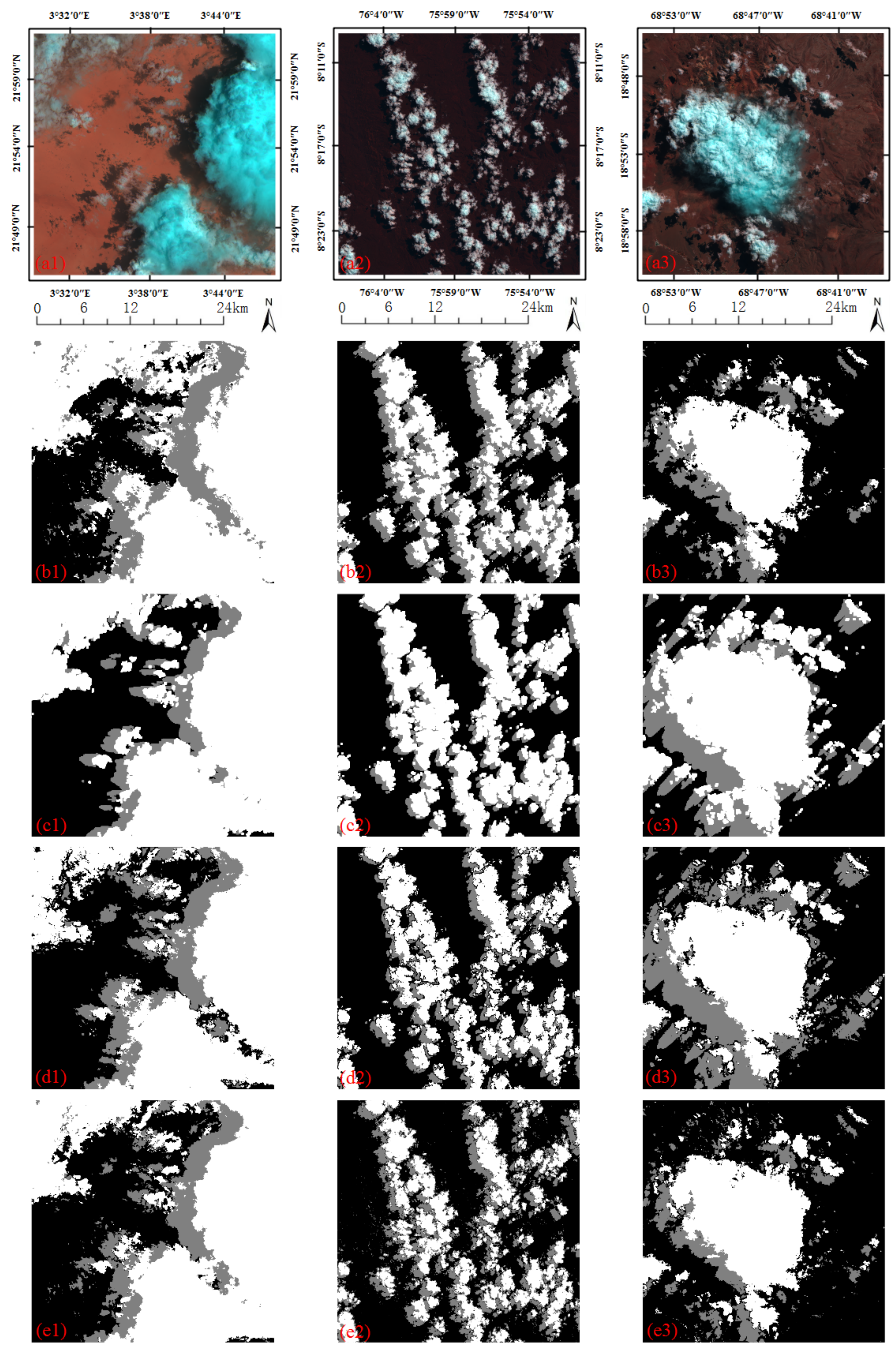
We compare our method with two other cloud and cloud shadow detection methods including Zhu’s method [23] and Li’s method [32]. Figure 7 shows several cloud and cloud shadow detection instances, where (a1–a3) is the original image, (b1–b3) is ground truth, white represents the cloud, gray represents the cloud shadow and black represents the non-cloud, (c1–c3)–(e1–e3) are the results of two compared methods and our method. It can be observed that all three cloud detection methods can effectively detect the clouds and their shadows. In addition, compared to the cloud shadow detection results, the cloud detection results are more accurate. The statistical results in

Table 5. Statistical results of different cloud and cloud shadow detection methods.

Methods	OA	Precision_c	Recall_c	Precision_s	Recall_s
Zhu’s method [23]	0.8771	0.8062	0.9272	0.4956	0.3686
Li’s method [32]	0.8895	0.8367	0.8847	0.5459	0.5137
Proposed method	0.9116	0.8914	0.8933	0.5588	0.5486

also confirm the conclusions above. From Table 5, we can see that our method obtains the highest OA, Precision_c, Precision_s and Recall_s, which indicates that the proposed method is effective for cloud and cloud shadow detection.

4. Conclusions

In this paper, a novel cloud detection method is proposed for the multispectral remote sensing images from Landsat 8. Clouds are obvious and easily distinguished from snow and ice in the color composite image of Bands 6, 3 and 2, and SLIC method is firstly used to cluster the color composite image into superpixel sub-regions. In these superpixels, the bright and thick cloud superpixels, as well as obvious non-cloud superpixels, are easily identified. Therefore, we use a threshold function in brightness feature space to distinguish the obvious cloud and non-cloud superpixels from the potential cloud superpixels, thus speeding up the detection. Potential cloud superpixels usually include dark clouds, semi-transparent thin clouds and bright non-clouds, which are easily misclassified. In this paper, a double-branch PCANet is designed to retrieve the high-level features of clouds, then combined with a linear SVM classifier, the classes of potential cloud superpixels are predicted. Through the two-step superpixel classification strategy, all the superpixels in the image are predicted as cloud or non-cloud. Considering the sub-region-based method will cause misclassified pixels, a fully connected CRF model is employed as the post-processing step to refine the final classification result. Because CRF processing is based on pixel and the optimization is global, the final extracted cloud borders are more accurate. Quantitative and qualitative experiments are performed on the L8 CCA dataset. Results demonstrate that, compared with other state-of-the-art methods, the proposed method can correctly detect cloud under different scenes. In addition, it can effectively distinguish the cloud with from snow and ice. In the future, we will take more information into consideration to further improve the accuracy of our cloud detection method. For example, we will consider the cloud shadow as it always occur in pairs with cloud. In addition, we will adapt our work to detect thin cloud, thick cloud, cloud shadow, ice/snow and water simultaneously.

References

- Pankiewicz, G.S. Pattern recognition techniques for the identification of cloud and cloud systems. Meteorol. Appl. 1995, 2, 257–271. [Google Scholar] [CrossRef]
- Zhu, Z.; Woodcock, C.E. Continuous change detection and classification of land cover using all available Landsat data. Remote Sens. Environ. 2014, 144, 152–171. [Google Scholar] [CrossRef]
- Chen, N.; Li, J.; Zhang, X. Quantitative evaluation of observation capability of GF-1 wide field of view sensors for soil moisture inversion. J. Appl. Remote Sens. 2015, 9, 199–203. [Google Scholar] [CrossRef]
- Lu, C.; Bai, Z. Characteristics and typical applications of GF-1 satellite. In Proceedings of the 2015 IEEE International Geoscience and Remote Sensing Symposium (IGARSS 2015), Milan, Italy, 26–31 July 2015; pp. 1246–1249. [Google Scholar] [CrossRef]
- Xu, X.; Shi, Z.; Pan, B. l0-based sparse hyperspectral unmixing using spectral information and a multi-objectives formulation. ISPRS J. Photogramm. Remote Sens. 2018, 141, 46–58. [Google Scholar] [CrossRef]
- Stubenrauch, C.; Rossow, W.B.; Kinne, S.; Zhao, G. GEWEX cloud assessment: A review. International Radiation Symposium: Radiation Processes in the Atmosphere and Ocean (IRS 2012), Berlin, Germany, 6–10 August 2012; pp. 404–407. [Google Scholar] [CrossRef]
- Saunders, R.W. An automated scheme for the removal of cloud contamination from AVHRR radiances over western Europe. Int. J. Remote Sens. 1986, 7, 867–886. [Google Scholar] [CrossRef]
- Zhu, Z.; Woodcock, C.E. Automated cloud, cloud shadow, and snow detection in multitemporal Landsat data: An algorithm designed specifically for monitoring land cover change. Remote Sens. Environ. 2014, 152, 217–234. [Google Scholar] [CrossRef]
- Shao, Z.; Deng, J.; Wang, L.; Fan, Y.; Sumari, N.S.; Cheng, Q. Fuzzy AutoEncode based cloud detection for remote sensing imagery. Remote Sens. 2017, 9, 311. [Google Scholar] [CrossRef]
- Jedlovec, G.J.; Haines, S.L.; LaFontaine, F.J. Spatial and temporal varying thresholds for cloud detection in GOES imagery. IEEE Trans. Geosci. Remote Sens. 2008, 46, 1705–1717. [Google Scholar] [CrossRef]
- Jin, S.M.; Homer, C.; Yang, L.M.; Xian, G.; Fry, J.; Danielson, P.; Townsend, P.A. Automated cloud and shadow detection and filling using two-date Landsat imagery in the USA. Int. J. Remote Sens. 2013, 34, 1540–1560. [Google Scholar] [CrossRef]
- Goodwin, N.R.; Collett, L.J.; Denham, R.J.; Flood, N.; Tindall, D. Cloud and cloud shadow screening across Queensland, Australia: An automated method for landsat TM/ETM plus time series. Remote Sens. Environ. 2013, 134, 50–65. [Google Scholar] [CrossRef]
- Hagolle, O.; Huc, M.; Pascual, D.V.; Dedieu, G. A multi-temporal method for cloud detection, applied to FORMOSAT-2, VENμS, LANDSAT and SENTINEL-2 images. Remote Sens. Environ. 2010, 114, 1747–1755. [Google Scholar] [CrossRef] [Green Version]
- Chen, S.; Chen, X.; Chen, J.; Jia, P.; Cao, X.; Liu, C. An iterative haze optimized transformation for automatic cloud/haze detection of landsat imagery. IEEE Trans. Geosci. Remote Sens. 2016, 54, 2682–2694. [Google Scholar] [CrossRef]
- Qian, J.; Luo, Y.; Wang, Y.; Li, D. Cloud detection of optical remote sensing image time series using Mean Shift algorithm. In Proceedings of the 2016 IEEE International Geoscience and Remote Sensing Symposium (IGARSS 2016), Beijing, China, 10–15 July 2016; pp. 560–562. [Google Scholar] [CrossRef]
- Oreopoulos, L.; Wilson, M.J.; Várnai, T. Implementation on Landsat data of a simple cloud-mask algorithm developed for MODIS land bands. IEEE Geosci. Remote Sens. Lett. 2011, 8, 597–601. [Google Scholar] [CrossRef]
- Marais, I.V.; Du Preez, J.A.; Steyn, W.H. An optimal image transform for threshold-based cloud detection using heteroscedastic discriminant analysis. Int. J. Remote Sens. 2011, 32, 1713–1729. [Google Scholar] [CrossRef]
- Shao, Z.; Hou, J.; Jiang, M.; Zhou, X. Cloud detection in Landsat imagery for Antarctic region using multispectral thresholds. In Proceedings of the SPIE Asia Pacific Remote Sensing, Beijing, China, 13–16 October 2014. [Google Scholar] [CrossRef]
- Xie, F.; Shi, M.; Shi, Z.; Yin, J.; Zhao, D. Multilevel cloud detection in remote sensing images based on deep learning. IEEE J. Sel. Top. Appl. Earth Obs. Remote Sens. 2017, 10, 3631–3640. [Google Scholar] [CrossRef]
- Cihlar, J.; Howarth, J. Detection and removal of cloud contamination from AVHRR images. IEEE Trans. Geosci. Remote Sens. 1994, 32, 583–589. [Google Scholar] [CrossRef]
- Irish, R.R. Landsat 7 automatic cloud cover assessment. Proc. SPIE Int. Soc. Opt. Eng. 2000, 4049, 348. [Google Scholar] [CrossRef]
- Zhu, Z.; Woodcock, C.E. Object-based cloud and cloud shadow detection in Landsat imagery. Remote Sens. Environ. 2012, 118, 83–94. [Google Scholar] [CrossRef]
- Zhu, Z.; Wang, S.; Woodcock, C.E. Improvement and expansion of the Fmask algorithm: Cloud, cloud shadow, and snow detection for Landsats 4–7, 8, and Sentinel 2 images. Remote Sens. Environ. 2015, 159, 269–277. [Google Scholar] [CrossRef]
- Yang, Y.; Zheng, H.; Chen, H. Automated cloud detection algorithm for multi-spectral high spatial resolution images using Landsat-8 OLI. In Advances in Image and Graphics Technologies; Tan, T., Ruan, Q., Wang, S., Ma, H., Di, K., Eds.; Springer: Berlin/Heidelberg, Germany, 2015; pp. 396–407. [Google Scholar]
- Zhu, Z.; Woodcock, C.E.; Holden, C.; Yang, Z. Generating synthetic Landsat images based on all available Landsat data: Predicting Landsat surface reflectance at any given time. Remote Sens. Environ. 2015, 162, 67–83. [Google Scholar] [CrossRef]
- Tan, K.; Zhang, Y.; Tong, X. Cloud extraction from chinese high resolution satellite imagery by probabilistic latent semantic analysis and object-based machine learning. Remote Sens. 2016, 8, 963. [Google Scholar] [CrossRef]
- Ren, R.Z.; Gu, L.J.; Wang, H.F. Clouds and clouds shadows detection and matching in modis multispectral satellite images. In Proceedings of the 2012 International Conference on Industrial Control and Electronics Engineering (ICICEE 2012), Xi’an, China, 23–25 August 2012; pp. 71–74. [Google Scholar] [CrossRef]
- Surya, S.R.; Simon, P. Automatic cloud detection using spectral rationing and fuzzy clustering. In Proceedings of the 2013 Second International Conference on Advanced Computing, Networking and Security (ADCONS 2013), Mangalore, India, 15–17 December 2013; pp. 90–95. [Google Scholar] [CrossRef]
- Kong, X.; Qian, Y.; Zhang, A. Cloud and shadow detection and removal for Landsat-8 data. In Proceedings of the 8th Symposium on Multispectral Image Processing and Pattern Recognition (MIPPR 2013), Wuhan, China, 26–27 October 2013. [Google Scholar] [CrossRef]
- Danda, S.; Challa, A.; Sagar, B.S.D. A morphology-based approach for cloud detection. In Proceedings of the 2016 IEEE International Geoscience and Remote Sensing Symposium (IGARSS 2016), Beijing, China, 10–15 July 2016; pp. 80–83. [Google Scholar] [CrossRef]
- Fisher, A. Cloud and cloud-shadow detection in spot5 hrg imagery with automated morphological feature extraction. Remote Sens. 2014, 6, 776–800. [Google Scholar] [CrossRef]
- Li, Z.; Shen, H.; Li, H.; Xia, G.; Gamba, P.; Zhang, L. Multi-feature combined cloud and cloud shadow detection in GaoFen-1 wide field of view imagery. Remote Sens. Environ. 2017, 191, 342–358. [Google Scholar] [CrossRef] [Green Version]
- Taravat, A.; Del Frate, F.; Cornaro, C.; Vergari, S. Neural networks and support vector machine algorithms for automatic cloud classification of whole-sky ground-based images. IEEE Geosci. Remote Sens. Lett. 2015, 12, 666–670. [Google Scholar] [CrossRef]
- Bai, T.; Li, D.R.; Sun, K.M.; Chen, Y.P.; Li, W.Z. Cloud detection for high-resolution satellite imagery using machine learning and multi-feature fusion. Remote Sens. 2016, 8, 715. [Google Scholar] [CrossRef]
- Hu, X.; Wang, Y.; Shan, J. Automatic recognition of cloud images by using visual saliency features. IEEE Geosci. Remote Sens. Lett. 2015, 12, 1760–1764. [Google Scholar] [CrossRef]
- Li, P.; Dong, L.; Xiao, H.; Xu, M. A cloud image detection method based on SVM vector machine. Neurocomputing 2015, 169, 34–42. [Google Scholar] [CrossRef]
- An, Z.; Shi, Z. Scene learning for cloud detection on remote-sensing images. IEEE J. Sel. Top. Appl. Earth Obs. Remote Sens. 2015, 8, 4206–4222. [Google Scholar] [CrossRef]
- Krizhevsky, A.; Sutskever, I.; Hinton, G.E. Imagenet classification with deep convolutional neural networks. In Proceedings of the 25th International Conference on Neural Information Processing Systems, Lake Tahoe, NV, USA, 3–6 December 2012; pp. 1097–1105. [Google Scholar]
- Simonyan, K.; Zisserman, A. Very deep convolutional networks for large-scale image recognition. In Proceedings of the 2015 International Conference on Learning Representations (ICLR), San Diego, CA, USA, 7–9 May 2015. [Google Scholar]
- He, K.; Zhang, X.; Ren, S.; Sun, J. Deep residual learning for image recognition. In Proceedings of the 2016 IEEE Conference on Computer Vision and Pattern Recognition (CVPR), Lake Tahoe, NV, USA, 26 June–1 July 2016; pp. 770–778. [Google Scholar] [CrossRef]
- Pan, B.; Shi, Z.; Xu, X. MugNet: Deep learning for hyperspectral image classification using limited samples. ISPRS J. Photogramm. Remote Sens. 2017. [Google Scholar] [CrossRef]
- Johnston, T.; Young, S.R.; Hughes, D.; Patton, R.M.; White, D. Optimizing convolutional neural networks for cloud detection. In Proceedings of the 2017 Machine Learning on HPC Environments (MLHPC 17), Denver, CO, USA, 12–17 November 2017; pp. 1–9. [Google Scholar] [CrossRef]
- Zhang, Z.; Iwasaki, A.; Xu, G.; Song, J. Small satellite cloud detection based on deep learning and image compression. Preprints 2018. [Google Scholar] [CrossRef]
- Shi, M.; Xie, F.; Zi, Y.; Yin, J. Cloud detection of remote sensing images by deep learning. In Proceedings of the 2016 IEEE International Geoscience and Remote Sensing Symposium (IGARSS 2016), Beijing, China, 10–15 July 2016; pp. 701–704. [Google Scholar] [CrossRef]
- Goff, M.; Tourneret, J.; Wendt, H.; Ortner, M.; Spigai, M. Deep learning for cloud detection. In Proceedings of the 8th International Conference on Pattern Recognition Systems (ICPRS 2017), Madrid, Spain, 11–13 July 2017; pp. 1–6. [Google Scholar] [CrossRef]
- Ozkan, S.; Efendioglu, M.; Demirpolat, C. Cloud detection from rgb color remote sensing images with deep pyramid networks. arXiv, 2018; arXiv:1801.08706. [Google Scholar]
- Xiao, Z. Study on Cloud Detection Method for High Resolution Satellite Remote Sensoring Image; Harbin Institute of Technology: Heilongjiang, China, 2013. [Google Scholar]
- Achanta, R.; Shaji, A.; Smith, K.; Lucchi, A.; Fua, P.; SüSstrunk, S. SLIC superpixels compared to state-of-the-art superpixel methods. IEEE Trans. Pattern Anal. Mach. Intell. 2012, 34, 2274–2282. [Google Scholar] [CrossRef] [PubMed]
- Philipp, K.; Koltun, V. Efficient inference in fully connected CRFs with gaussian edge potentials. In Proceedings of the 24th International Conference on Neural Information Processing Systems, Granada, Spain, 12–15 December 2011; pp. 109–117. [Google Scholar]
- U.S. Geological Survey. Available online: https://landsat.usgs.gov/using-usgs-landsat-8-product (accessed on 13 April 2018).
- Foga, S.; Scaramuzza, P.L.; Guo, S.; Zhu, Z.; Dilley, R.D.; Beckmann, T.; Schmidt, G.L.; Dwyer, J.L.; Joseph Hughes, M.; Laue, B. Cloud detection algorithm comparison and validation for operational Landsat data products. Remote Sens. Environ. 2017, 194, 379–390. [Google Scholar] [CrossRef] [Green Version]
- Chan, T.H.; Jia, K.; Gao, S.; Lu, J.; Zeng, Z.; Ma, Y. PCANet: A simple deep learning baseline for image classification IEEE Trans. Image Process. 2015, 24, 5017–5032. [Google Scholar] [CrossRef] [PubMed]
- Pan, B.; Shi, Z.; Zhang, N.; Xie, S. Hyperspectral image classification based on nonlinear spectral-spatial network. IEEE Geosci. Remote Sens. Lett. 2016, 13, 1782–1786. [Google Scholar] [CrossRef]
- Jarrett, K.; Kavukcuoglu, K.; Ranzato, M.; LeCun, Y. What is the best multi-stage architecture for object recognition? In Proceedings of the 2009 IEEE International Conference on Computer Vision (ICCV), Kyoto, Japan, 29 September–2 October 2009; pp. 2146–2153. [Google Scholar] [CrossRef]
- Kavukcuoglu, K.; Sermanet, P.; Boureau, Y.; Gregor, K.; Mathieu, M.; Lecun, Y. Learning convolutional feature hierarchies for visual recognition. In Proceedings of the 23th International Conference on Neural Information Processing Systems, Vancouver, BC, Canada, 6–9 December 2010; pp. 1090–1098. [Google Scholar]
- G<i>ó</i>mez-Chova, L.; Camps-Valls, G.; Calpe-Maravilla, J.; Guanter, L.; Moreno, J. Cloud-screening algorithm for ENVISAT/MERIS multispectral images. IEEE Trans. Geosci. Remote Sens. 2007, 45, 4105–4118. [Google Scholar] [CrossRef]
- Zhang, Y.; Guindon, B.; Cihlar, J. An image transform to characterize and compensate for spatial variations in thin cloud contamination of Landsat images. Remote Sens. Environ. 2002, 82, 173–187. [Google Scholar] [CrossRef]
- Zhang, Q.; Xiao, C. Cloud detection of RGB color aerial photographs by progressive refinement scheme. IEEE Trans. Geosci. Remote Sens. 2014, 52, 7264–7275. [Google Scholar] [CrossRef]
- Chen, L.C.; Papandreou, G.; Kokkinos, I.; Murphy, K.; Yuille, A.L. DeepLab: Semantic image segmentation with deep convolutional nets, atrous convolution, and fully connected CRFs. IEEE Trans. Pattern Anal. Mach. Intell. 2017, 40, 834–848. [Google Scholar] [CrossRef] [PubMed]
Figure 1.
Flow chart of the proposed cloud detection method.
Figure 2.
Example of superpixel segmentation. (a) Original color composite image. (b) SLIC segmentation result. (c) Superpixel coarse classification result (white represents the cloud, black represents the non-cloud and gray represents the potential cloud). (d) Two-step superpixel classification result. (e) Fully connected CRF refinement result.
Figure 3.
Cumulative histogram of brightness feature b.
Figure 4.
Flow chart of the cloud detection process based on PCANet.
Figure 5.
Visual comparisons of cloud detection results of different frameworks. (a1,a2) Color composite images (a1 and a2 are subsets of Landsat 8 images LC81930452013126LGN01 and LC82290572014141LGN00, respectively). (b1,b2) Ground truth. (c1,c2) Results of the simple double- branch PCANet. (d1,d2) Results of the two-step superpixel classification strategy. (e1,e2) Results of the two-step strategy combined with guided filter. (f1,f2) Results of our proposed framework.
Figure 6.
Visual comparisons of cloud detection results of different methods. (a1–a3) Original color composite images (a1: LC81330312013202LGN00; a2: LC80211222013361LGN00; a3: LC81030162014107LGN00). (b1–b3) Ground truth. (c1–c3) Zhu’s method. (d1–d3) Yang’s method. (e1–e3) Li’s method. (f1–f3) Shi’s method. (g1–g3) Goff’s method. (h1–h3) The proposed method.
Figure 7.
Visual comparisons of cloud and cloud shadow detection results of different methods. (a1–a3) Original color composite images (a1–a3 are subsets of Landsat 8 images LC81930452013126LGN01, LC80070662014234LGN00 and LC80010732013109LGN00, respectively). (b1–b3) Ground truth (white represents the cloud, gray represents the cloud shadow and black represents the non-cloud). (c1–c3) Zhu’s method. (d1–d3) Li’s method. (e1–e3) The proposed method.