Historical and Operational Monitoring of Surface Sediments in the Lower Mekong Basin Using Landsat and Google Earth Engine Cloud Computing

Abstract

Reservoir construction and land use change are altering sediment transport within river systems at a global scale. Changes in sediment transport can impact river morphology, aquatic ecosystems, and ultimately the growth and retreat of delta environments. The Lower Mekong Basin is crucial to five neighboring countries for transportation, energy production, sustainable water supply, and food production. In response, countries have coordinated to develop programs for regional scale water quality monitoring that including surface sediment concentrations (SSSC); however, these programs are based on a limited number of point measurements and due to resource limitations, cannot provide comprehensive insights into sediment transport across all strategic locations within the Lower Mekong Basin. To augment in situ SSSC data from the current monitoring program, we developed an empirical model to estimate SSSC across the Lower Mekong Basin from Landsat observations. Model validation revealed that remotely sensed SSSC estimates captured the spatial and temporal dynamics in a range of aquatic environments (main stem of Mekong river, tributary systems, Mekong Floodplain, and reservoirs) while, on average, slightly underestimating SSSC by about 2 mg·L${}^{-1}$ across all settings. The operational SSSC model was developed and implemented using Google Earth Engine and Google App Engine was used to host an online application that allows users, without any knowledge of remote sensing, to access SSSC data across the region. Expanded access to SSSC data should be particularly helpful for resource managers and other stakeholders seeking to understand the dynamics between surface sediment concentrations and land use conversions, water policy, and energy production in a globally strategic region.

1. Introduction

Human activities such as agriculture, forestry, and urbanization are increasing sediment transport in rivers globally, while reservoir construction is simultaneously decreasing the total sediment flux to coastal environments [1]. Because sediment transport by rivers impacts channel morphology, aquatic ecosystems, reservoir storage capacity, and ultimately the growth or retreat of delta environments [2]; monitoring changes in sediment concentration and transport is critical to effective basin management. Timely information on total suspended matter is critical for land managers to assess the effects of a wide range of issues caused by poor water quality. Unfortunately, collection of reliable suspended sediment concentration data at the spatial and temporal resolution necessary for effective basin management and planning can often be prohibitively time consuming and expensive in large rivers.

The Mekong River is the largest trans-boundary river basin in Asia that covers an area of 795,000 km${}^2$, and has an annual discharge of 475 km${}^3$ [3]. Each year the Mekong delivers approximately 160 million tons of sediment to the South China Sea [4]. The Mekong River hydrology is dominated by the seasonality of snowmelt runoff into the northern headwaters on the Tibetan Plateau, and the seasonal monsoon in the lower basin. The lowest flows are between February and April, with peak discharge between August and September. The Mekong River Basin is rapidly developing and due to increasing demands for hydropower and freshwater, reservoir construction has accelerated in recent decades [5] with potential to alter sediment transport in the region [6,7]. Changes in the Mekong river sediment supply, most likely caused by dam retention of sediment and channel-bed sand extraction in the Mekong delta, are suspected to be the cause of erosion patterns observed in the Mekong delta [2]. However, while changes in sediment transport have been observed on other major Asian rivers such as the Indus, Yellow, and Yangtze Rivers, limited field data has made it difficult to detect changes in sediment discharge on the Lower Mekong River, despite the fact that the Lower Mekong Basin is experiencing similar pressures of population growth, land use change, infrastructure development, and reservoir construction [8].

The most comprehensive field dataset for suspended sediments in the Lower Mekong has been collected by The Mekong River Commission (MRC). Suspended sediment is a water quality constituent of particular concern to MRC because suspended sediments increase turbidity and can influence the transport of particle bound contaminants such as nutrients, organic compounds, pesticides, and trace metals. In addition, suspended sediments are critical to the accumulation of wetland soils in the Mekong Delta [9]. The MRC has an extensive water quality monitoring network, with 132 stations across five countries in the Lower Mekong Basin (Thailand, Vietnam, Laos PDR, Cambodia, and Myanmar) (Figure 1). At a number of stations samples have been collected monthly since 1985, however there are significant gaps in the records at numerous stations. While the MRC dataset on suspended matter provides invaluable information on water quality in the Lower Mekong Basin, it consists of single point measurements taken from the surface of the river at a single point in the river cross section, and therefore the dataset provides limited understanding of the spatial distribution of suspended sediments along the river.

Remote sensing tools can provide spatial and temporal resolution for surface suspended sediment concentration (SSSC) in large rivers that are not available from traditional in situ measurements [10,11,12,13]. The retrieval of SSSC from remote sensing systems relies on the optical properties (transmittance, absorption and scattering) of water and the dissolved and suspended constituents in the water. Suspended solids are responsible for most of the scattering in an aquatic system, whereas chlorophyll-a (chl-a) and colored dissolved matter are mainly responsible for absorption [14]. A variety of techniques have been used to estimate SSSC from different remote sensing systems [15,16,17]. There is a wide body of research on assessing water quality analytical optical modeling using in situ inherent optical properties [18,19,20]. Unfortunately, these approaches are often complex, iterative and location specific, leading researchers to explore the extent to which empirical models can provide robust estimates of water quality parameters. Methods used to relate in situ data to the satellite observations through statistical relationships include simple linear regression, non-linear regressions, principal component analysis, and neural networks. Previous studies have shown that SSSC is well correlated with the first four bands of the Landsat sensors [21,22,23] and the use of a single band from the sensor series, provided the band is chosen appropriately, can provide a robust estimation of SSSC [24,25,26,27,28,29]. Moreover, other studies have also illustrated the utility of band ratios from Landsat sensors to estimate SSSC [11,30,31]. Sensors from the Landsat satellite series (TM, ETM+, OLI) are the most commonly used remote sensing platforms for estimating SSSC [32].

Because the relationship between SSSC and surface reflectance is a function of sediment mineralogy, color, and grain size distribution [33], empirical models perform best when calibrated with local in situ observations. This is particularly important in riverine SSSC studies because there is often considerable spatial and temporal variability in these parameters. Previous efforts to estimate SSSC and TSS from remote sensing data sources in the Lower Mekong Basin have focused on the main stem of the Mekong River or on the Mekong Delta, but not both. For example, Suif et al. [34] developed an empirical model using the near-infrared band on Landsat TM as well as the blue, green, and red bands in a multiple linear regression along the Mekong River. In another recent study, Duc et al. [35] found a strong correlation between the 1st principle component of Landsat TM and ETM+ imagery and SSSC in the Mekong Delta. While these studies provide models to estimate SSSC accurately from remotely sensed data, the models were not validated at regional scale and therefore, need careful consideration before broad use. Other studies, such as Bui et al. [36] have used soil erosion modeling to estimate sediment transport dynamics within watersheds in Southeast Asia. Although, modeling approaches produce suspended sediment load (SSL) information irrespective of remote sensing inputs, the models require detailed parameterization and quality in situ data to accurately estimate SSL, which can limit application in data sparse regions.

Cloud based remote sensing platforms such as Google Earth Engine (GEE) offer exciting new opportunities to provide policy makers with high resolution near real-time SSSC data through a simple web interface without the need for expensive software, technical expertise or other resource demanding solutions. The goals of this study were to (1) calibrate a regional remote sensing model of SSSC in the Lower Mekong which augments the spatial and temporal resolution of existing field records and (2) develop an online application that allows users, without any expert knowledge of remote sensing, to monitor and analyze trends in SSSC for decision making within the region. We accomplished these goals by utilizing the extensive MRC SSSC dataset across the entire Lower Mekong Basin to develop an empirical model for estimating SSSC from satellite data. The model includes 8 main stem gauging stations on the Mekong River, and 36 additional gauging stations from tributary systems, the Mekong Floodplain, and reservoirs. The model is accessible through an operational online application that allows users to monitor and analyze trends in SSSC from continuously updated remote sensing datasets in a timely manner. This novel web application can provide actionable SSSC data to decision makers throughout the region.

2. Data and Methods

In this study we correlated in situ SSSC measurements with coinciding Landsat observations to create an empirical model to estimate SSSC in the Lower Mekong Basin. Due to large data volume and processing needs, GEE [37] was used to facilitate data processing. GEE allows users to run algorithms on georeferenced imagery, vector data, and other precomputed value-added products stored on Google’s cloud-based infrastructure in an easy-to-use manner. GEE was used in this study to (1) query all Landsat observations over the Mekong Basin that coincide with in situ measurements; (2) extract the spectra to develop an empirical SSSC model and (3) provide back-end processing for an online suspended sediment application. Figure 2 displays the overarching workflow used in this study.

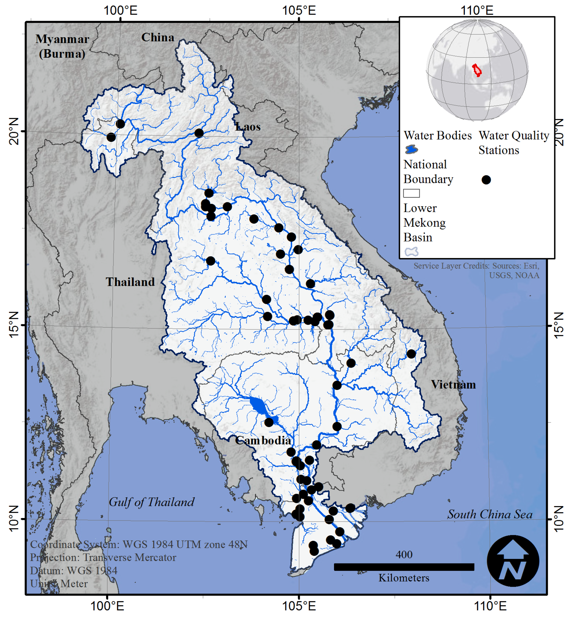
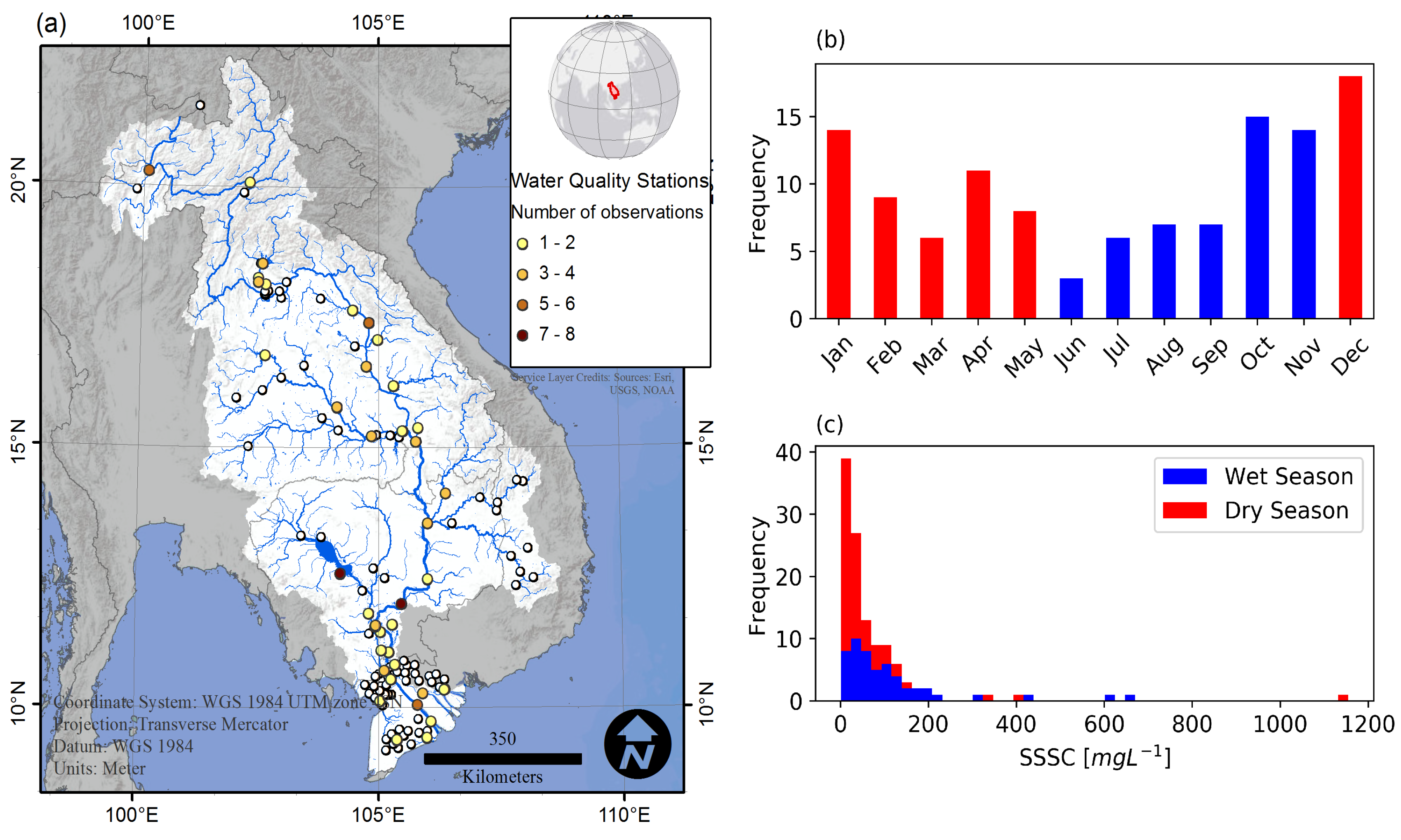
2.1. Field Measurement of Suspended Sediment Concentration

The reference dataset used to create and validate the SSSC model was acquired from the MRC data portal (http://portal.mrcmekong.org/). The MRC established a water quality monitoring network in 1985 to measure discharge and collect monthly water quality samples for a wide suite of constituents including cations, anions, nutrients and SSSC [38]. SSSC samples are collected near the surface (0.3–0.5 m) using a bottle, and therefore likely underestimate SSSC given that suspended sediment concentration typically increases with depth. Nevertheless, these surface samples provide an excellent comparison with remotely sensed optical properties which are most representative of shallow depths. Although this is the best available water quality dataset for the Lower Mekong Basin, it does include uncertainties in sampling technique consistency and quality from earlier collection years. At many stations, SSSC records are not complete, with data gaps ranging from months to years. For a thorough discussion of SSSC data reliability in the Lower Mekong Basin see Walling [8].

2.2. Landsat Collection Data

Data from the Landsat TM (from both Landsat 4 and 5 satellites), ETM+ (Landsat 7) and OLI (Landsat 8) sensors were used to estimate SSSC for water bodies in the Lower Mekong Basin. The Landsat 4, 5, 7, and 8 satellites are each in a sun-synchronous orbit each with a 16-day revisit time. Landsat 4 had an operating lifetime from 1982-1994, Landsat 5’s lifetime was from 1984–2011, and Landsat 7 has been active since its launch in 1999. Landsat 8, the most recent satellite in the series, was launched in 2013. While any two Landsat satellites were in operation, there was an 8-day offset of data acquisition between the two satellites increasing the temporal resolution. The TM, ETM+, and OLI sensors collect spectral channel data in the visible, near-infrared (NIR), and short-wave infrared (SWIR) portions of the electromagnetic spectrum at 30 × 30 m resolution. Landsat data collected from 1985 to 2011 from Landsat 4, 5, and 7 were used in this study to maximize the number of Landsat observations that coincide with the in situ data from MRC. All Landsat sensors are used within the online applications.

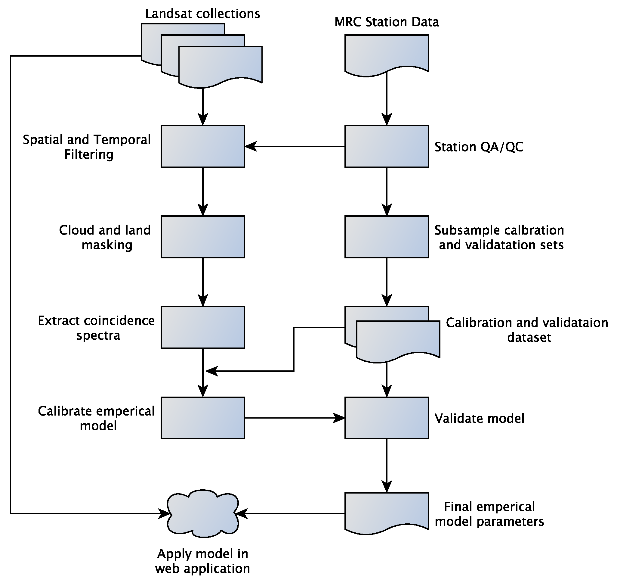
2.3. Data Preprocessing

The in situ data were provided as a table with geographic latitude and longitude along with suspended sediment concentration for each collection time. To reduce the influence of the channel bottom or upwelling that occurs next to the bank and in shallow waters, station locations were filtered to ensure that only stations at least 60 m (two Landsat pixels) from the bank of the waterbody were included in further analysis. To account for changes in river morphology during the time from 1985–2011, the shoreline was dynamically calculated from the European Commission’s Joint Research Center (JRC) Monthly Water History v1.0 image collection (JRC/GSW1_0/MonthlyHistory) [39] for each in situ collection date. Landsat or in situ data that was collected within 60m of the dynamic shoreline was not used in the analysis.

Next, the Landsat collections within GEE were queried to identify scene IDs that overlap MRC stations within one day of a in situ collection date. The precomputed surface reflectance (SR) Landsat collections were used in this analysis (LANDSAT/LT04/C01/T1_SR; LANDSAT/LT05/C01/T1_SR; LANDSAT/LE07/C01/T1_SR); these Landsat data collections have been converted from raw digital numbers to Top of Atmosphere (TOA) reflectance using the methods and band specific irradiance values from Chander et al. [40].

Atmospheric correction is an important process for the remote sensing of water quality as water-leaving radiance constitutes a small fraction of the total energy measured by the sensor, with the main contribution coming from the atmosphere [41]. Studies have found that image-based [42,43,44], site-specific [41,45,46], and radiative transfer model [47,48,49] atmospheric correction methods can provide adequate retrievals of surface reflectance for water quality mapping. The Landsat data used in this study have been atmospherically corrected using the Earth Resources Observation and Science (EROS) Center Science Processing Architecture (ESPA) surface reflectance processing system. The ESPA surface reflectance processing system uses the Landsat ecosystem disturbance adaptive processing system (LEDAPS) algorithm [50] to atmospherically correct data from Landsat 4–7. The LEDAPS processing algorithm is built upon the 6S atmospheric correction model [51,52]. The 6S atmospheric correction model is a single layer radiative transfer model that enables accurate simulations of satellite observations that account for the elevation of targets, includes the modeling of a realistic molecular/aerosol/mixed atmosphere, allows for the retrieval values from Lambertian or anisotropic ground surfaces, and includes the calculation of gaseous absorption [53]. Furthermore, the 6S model is a widely used and heavily documented radiative transfer code that has been rigorously validated [54,55] and applied for remote sensing of water quality [56,57,58] making it a suitable atmospheric correction procedure.

Included in the ESPA surface reflectance processing is the C Function of the Mask (CFMask) algorithm [59] used to map cloud, cloud confidence, cloud shadow, and snow/ice pixels in Landsat scenes. The CFMask is an implementation of the FMask algorithm [60] written in C programming language. The CFMask code is a multi-pass algorithm that first labels pixels based on a decision trees classifier; it then uses scene-wide statistics to validate or discard the initial pixel labels.The cloud shadow mask is created by iteratively projecting clouds to the ground with multiple cloud heights. Pixels flagged as cloud or cloud shadow were masked in the Landsat data collection using the CFMask pixel QA band. To ensure that the extracted image spectra were water, the JRC water mask [39] was used to extract water only pixels for analysis. The JRC Monthly Water History v1.0 image collection (JRC/GSW1_0/MonthlyHistory) was temporally filtered for the month coinciding with each individual Landsat scene and used to mask land pixels. The JRC data is only available from 16 March 1984 to 18 October 2015 which affects data processing outside of the JRC date range. Thus, the CFMask QA band was used to extract pixels flagged as water as a secondary/backup algorithm for Landsat scenes that fall out of the JRC data availability.

After the MRC station-satellite acquisition coincidence check and data masking, the image spectra were extracted from the coinciding and masked Landsat scenes. After the preprocessing and spectra extraction, a natural logarithmic transform was applied to both the atmospherically corrected image spectra and in situ SSSC measurements to reduce skewness and make the distributions more Gaussian for linear statistical modeling. The log transformed image spectra and SSSC measurements were then used to create an empirical model to estimate SSSC from Landsat imagery.

2.4. Statistical Methods

The total sample of image spectra and SSSC measurements was sub-setted into calibration and validation samples; 70% of the data were used for calibration and 30% were used for validation. The sub-setting was completed using a Monte Carlo approach where the validation data was randomly selected. The index of the samples selected for validation were stored for 10,000 iterations. The final validation sample was selected by finding 30% of the data indices that were selected the most from all Monte Carlo simulations, data not selected for the validation sample were used within the calibration sample.

To determine the optimal band or combination of bands for the model [32], the spectral data from visible and NIR bands and all possible visible and NIR band ratios were correlated to the calibration sample. Only the bands and band ratios that had an absolute linear correlation greater than 0.50 were used to test for the best covariate for estimating SSSC. The selected bands were then used to derive an empirical model of SSSC from the calibration dataset. Five statistical models were optimized between the image spectra and SSSC measurements using the Scientific Python (SciPy) module [61,62] in a local Python environment; these models include: (1) linear; (2) exponential; (3) 2nd order polynomial; (4) 3rd order polynomial and (5) 4th order polynomial functions. Each model was tested on the selected bands using the following objective functions: coefficient of determination (R${}^2$), sum of square error (SSE), and significance (p). The resulting model fit statistics were used to rank the best performing model based on the calibration dataset. The best performing model was then applied on the validation dataset and statistically analyzed to understand the accuracy and errors associated with estimating SSSC using the specified approach.

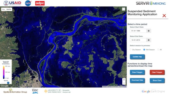
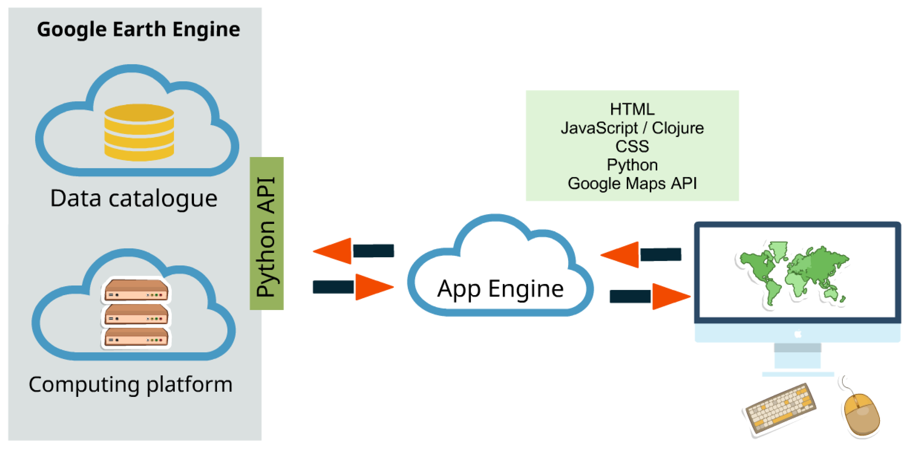
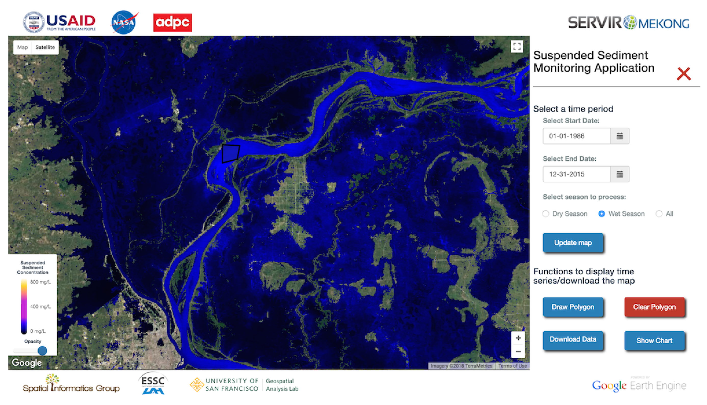
2.5. Online Application

The preprocessing methodology and selected empirical model of SSSC was implemented in an online application. Google’s App Engine was used to host the application that relies on the GEE backend to process the imagery. The framework for requesting data, performing spatial calculations, and serving the information in a browser is provided in Figure 3. The web interface relies on the Google App Engine technology, using elements of HTML, CSS and JavaScript (or Clojure). Requests from the front-end are made by a call from JavaScript to the Python script using Asynchronous JavaScript And XML (AJAX). The GEE Python library handles requests to GEE and receives the result. The information returned to the JavaScript is displayed in the browser. Spatial information is displayed with the Google Maps Application Programming Interface (API) and graphical data is displayed with the Google Visualization API.

3. Results

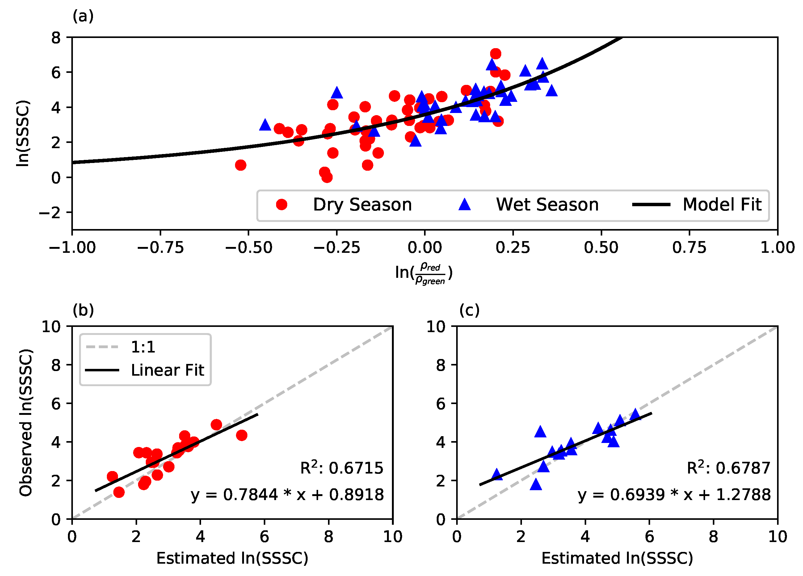
3.1. Model Calibration and Validation

From the original 132 MRC water quality stations, a total of 44 stations met our quality control criteria for having collections >60 m from the bank. (Figure 4). For the 44 selected MRC stations there were relatively few cloud-free, coinciding Landsat observations within one day of in situ sampling. Out of a total 24,749 in situ samples from the MRC dataset, a total of 118 Landsat observations met the criteria for inclusion in the empirical model across the 44 stations (see Appendix A for detailed information on the stations used). Figure 4 displays the spatial, temporal, and SSSC concentration distributions from the acquired coincidence samples. Overall, in situ samples and coincident Landsat observations were recovered from a variety of locations throughout the basin, but coincident observations were most common along the Mekong mainstem and larger tributary systems (Figure 4a). In total, the calibration dataset includes 8 stations located in the the Mekong River main stem, 11 stations located in tributary systems, 22 stations from the Mekong Floodplain (which constitutes all stations downstream from Kratie [35]), and 3 stations located within reservoirs (

Table A1. Table describing the 44 stations used in the study.

Station ID	Name	Lat.	Lon.	Waterbody	Type	Observations
H010501	Chiang Sean	20.2755	100.090986	Mekong River	Main stem	5
H013101	Nakhon Phanom	17.399339	104.800227	Mekong River	Main stem	6
H013401	Savannakhet	16.559887	104.743416	Mekong River	Main stem	3
H013801	Khong Chiam	15.32027	105.5	Mekong River	Main stem	2
H013900	Pakse	15.120617	105.78276	Mekong River	Main stem	3
H014501	Stung Treng	13.547263	106.015905	Mekong River	Main stem	4
H014901	Kratie	12.47827	106.015	Mekong River	Main stem	2
H019801	Chroy Chang Var	11.58483	104.9425	Mekong River	Main stem	4
H019802	Kampong Cham	12.001609	105.46783	Mekong River	Floodplain	8
H019804	My Thuan	10.277645	105.906339	Mekong River	Floodplain	4
H019805	My Tho	10.3444	106.35056	Mekong River	Floodplain	2
H019806	Neak Luong	11.59511	105.28694	Mekong River	Floodplain	1
H019807	Krom Samnor	11.069384	105.208978	Mekong River	Floodplain	1
H020101	Phnom Penh Port	11.57316	104.93167	Tonle Sap River	Floodplain	3
H020102	Prek Kdam	11.81319	104.8	Tonle Sap River	Floodplain	1
H020106	Kampong Luong	12.579697	104.213025	Tonle Sap Lake	Floodplain	7
H029812	Dai Ngai	9.733668	106.075538	Bassac River	Floodplain	2
H033401	Takhmao	11.564623	104.934383	Bassac River	Floodplain	3
H033402	Koh Khel	11.456477	105.039326	Bassac River	Floodplain	2
H033403	Khos Thom	11.105372	105.061034	Mekong River	Floodplain	3
H039801	Chau Doc	10.710065	105.124479	Bassac River	Floodplain	5
H039803	Can Tho	10.053218	105.800404	Bassac River	Floodplain	5
H039805	My Tho	10.35145	106.368236	Mekong River	Floodplain	1
H100101	Ban Hat Kham	20.084313	102.258378	Nam Ou River	Tributary	1
H230102	Tha Ngon	18.133752	102.621123	Nam Ngum River	Tributary	1
H230199	Nam Ngum at Damsite	18.53229	102.55333	Nam Ngum Reservoir	Reservoir	4
H231801	Nam Souang	18.25215	102.55333	Souang River	Tributary	2
H231901	Nam Houm	18.178159	102.55333	Nam Houm Reservoir	Reservoir	4
H290103	Ban Chai Buri	17.641781	104.461561	Nam Songkhram	Tributary	1
H320101	Se Bang Fai	17.076623	104.983587	Se Bang Fai	Tributary	2
H350101	Ban Keng Done	16.18774	105.316627	Se Bang Hieng	Tributary	2
H370104	Yasothon	15.783679	104.138624	Nam Chi	Tributary	4
H370299	Nam Pong Dam	16.77213	102.618581	Nam Pong	Reservoir	2
H380103	Ubon	15.223357	104.861663	Nam Mun	Tributary	4
H380128	Mun (Khong Chiam)	15.32194	105.51	Mekong River	Main stem	1
H390104	Souvanna Khili	15.385382	105.823818	Se Done	Tributary	1
H430102	Siempang	14.12097	106.3933	Se Kong	Tributary	3
H450101	Lumphat	13.552984	106.528211	Sre Pok	Tributary	1
H988102	Tan Thanh	10.81751	105.59028	Hong Ngu Canal	Floodplain	2
H988114	Tu Thuong	10.825895	105.339373	Tu Thuong Canal	Floodplain	2
H988202	My Thanh	9.429292	105.998322	My Thanh Canal	Floodplain	2
H988214	Phuoc Sinh	9.38372	105.38333	Quan Lo-Phung Hiep	Floodplain	2
H988302	Ba The	10.54331	105.25694	Kinh Ba The Canal	Floodplain	2
H988314	Soc Xoai	10.13242	105.02889	Rach Gia-Ha Tien	Floodplain	2

). The calibration and validation dataset includes 118 Landsat observations coincident with in situ SSSC measurements, 66 of these instances come from the dry season (December to May) , while 52 occurred during the wet season (June to November), providing a good representation of both the wet and dry seasons for statistical analysis (Figure 4b). The range of in situ SSSC values in the calibration dataset is 1.0–1155.0 mg·L${}^{-1}$ for the dry season and 8.0–655.0 mg·L${}^{-1}$ for the wet season (Figure 4c).

The statistical correlation analysis between SSSC and the Landsat spectra yielded five candidate bands for the empirical model creation and further analysis based on our criteria (

Table A2. Correlation matrix for the log spectral values of each band and ln(SSSC).

	${\mathit{\rho }}_{\mathit{Blue}}$	${\mathit{\rho }}_{\mathit{Green}}$	${\mathit{\rho }}_{\mathit{Red}}$	${\mathit{\rho }}_{\mathit{NIR}}$	$\frac{{\mathit{\rho }}_{\mathit{Blue}}}{{\mathit{\rho }}_{\mathit{Green}}}$	$\frac{{\mathit{\rho }}_{\mathit{Blue}}}{{\mathit{\rho }}_{\mathit{Red}}}$	$\frac{{\mathit{\rho }}_{\mathit{Blue}}}{{\mathit{\rho }}_{\mathit{NIR}}}$	$\frac{{\mathit{\rho }}_{\mathit{Green}}}{{\mathit{\rho }}_{\mathit{Red}}}$	$\frac{{\mathit{\rho }}_{\mathit{Green}}}{{\mathit{\rho }}_{\mathit{NIR}}}$	$\frac{{\mathit{\rho }}_{\mathit{Red}}}{{\mathit{\rho }}_{\mathit{NIR}}}$	SSSC [mg·L${}^{-1}$]
${\rho }_{Blue}$	1
${\rho }_{Green}$	0.911	1
${\rho }_{Red}$	0.826	0.961	1
${\rho }_{NIR}$	0.750	0.75	0.809	1
${\rho }_{Blue}/{\rho }_{Green}$	0.023	0.432	0.522	0.240	1
${\rho }_{Blue}/{\rho }_{Red}$	0.367	0.677	0.827	0.588	0.840	1
${\rho }_{Blue}/{\rho }_{NIR}$	0.230	0.345	0.468	0.816	0.334	0.544	1
${\rho }_{Green}/{\rho }_{Red}$	0.537	0.722	0.886	0.720	0.578	0.928	0.590	1
${\rho }_{Green}/{\rho }_{NIR}$	0.234	0.183	0.275	0.762	0.069	0.221	0.917	0.380	1
${\rho }_{Red}/{\rho }_{NIR}$	0.101	0.274	0.283	0.335	0.445	0.367	0.581	0.246	0.803	1
SSSC [mg L${}^{-1}$]	0.396	0.557	0.666	0.654	0.486	0.705	0.616	0.727	0.447	0.001	1

). The bands and band ratios with a correlation coefficient over 0.5 with the SSSC calibration dataset included: ${\rho }_{Green}$, ${\rho }_{Red}$, ${\rho }_{NIR}$, $\frac{{\rho }_{Blue}}{{\rho }_{Red}}$, $\frac{{\rho }_{Blue}}{{\rho }_{NIR}}$ and $\frac{{\rho }_{Green}}{{\rho }_{Red}}$. The $\frac{{\rho }_{Green}}{{\rho }_{Red}}$ band ratio yielded the highest absolute correlation of 0.73. Empirical model fitting found that a 4th order polynomial fit with the $\frac{{\rho }_{Red}}{{\rho }_{Green}}$ band ratio yielded the best fit ; however, to avoid overfitting we used an exponential model with similar fit statistics to estimate SSSC (

Table A3. Statistical modeling results for each combination of bands/ratios selected and fitting functions.

Band	Model	R${}^2$	SSE	p
${\rho }_{Green}$	Linear	0.305	98.84	<0.01
	Exponential	0.324	96.16	<0.01
	2nd order Polynomial	0.332	94.91	<0.01
	3rd order Polynomial	0.364	90.45	<0.01
	4th order Polynomial	0.372	89.37	<0.01
${\rho }_{Red}$	Linear	0.412	83.71	<0.01
	Exponential	0.453	77.93	<0.01
	2nd order Polynomial	0.468	75.67	<0.01
	3rd order Polynomial	0.472	75.08	<0.01
	4th order Polynomial	0.476	74.50	<0.01
${\rho }_{NIR}$	Linear	0.384	87.52	<0.01
	Exponential	0.370	89.74	<0.01
	2nd order Polynomial	0.385	87.52	<0.01
	3rd order Polynomial	0.386	87.35	<0.01
	4th order Polynomial	0.388	87.00	<0.01
${\rho }_{Red}/{\rho }_{Blue}$	Linear	0.430	81.15	<0.01
	Exponential	0.430	81.15	<0.01
	2nd order Polynomial	0.437	80.08	<0.01
	3rd order Polynomial	0.474	74.79	<0.01
	4th order Polynomial	0.476	74.55	<0.01
${\rho }_{Blue}/{\rho }_{NIR}$	Linear	0.306	98.51	<0.01
	Exponential	0.289	101.14	<0.01
	2nd order Polynomial	0.315	97.51	<0.01
	3rd order Polynomial	0.322	96.47	<0.01
	4th order Polynomial	0.323	96.29	<0.01
${\rho }_{Red}/{\rho }_{Green}$	Linear	0.463	76.45	<0.01
	Exponential	0.494	71.94	<0.01
	2nd order Polynomial	0.502	70.90	<0.01
	3rd order Polynomial	0.504	70.57	<0.01
	4th order Polynomial	0.505	70.46	<0.01

). The fitting procedure yielded the following equation to derive SSSC from Landsat $\frac{{\rho }_{Red}}{{\rho }_{Green}}$ band ratio:

$$y=1.904\times e^{1.448·x+0.630}$$

(1)

where y is the estimated ln(SSSC) and x is ln($\frac{{\rho }_{Red}}{{\rho }_{Green}}$). Equation (1) was applied to the validation sample subset and to determine the accuracy of the model (Figure 5). Model error statistics were calculated to quantify the performance of the model (Figure 5,

Table 1. Error statistics for validation of empirical model compared to the validation dataset.

Season	R [-]	Bias [mg·L${}^{-1}$]	RMSE [mg·L${}^{-1}$]	RE [%]	NSE [-]	Validation Data Range [mg·L${}^{-1}$]
Dry	0.82	−3.73	17.50	43.95	0.54	4.0–133.0
Wet	0.82	1.17	22.50	41.65	0.52	6.0–225.5
Total	0.84	−1.63	19.64	42.96	0.58	4.0–225.5

) by converting model output from log space to actual SSSC values. The validation dataset was split into wet and dry season observations in order to assess model performance under high flow and low flow conditions (Figure 5b,c). Model error statistics such as correlation coefficient (R) and Nash-Sutcliffe model efficiency coefficient (NSE) are well within acceptable model range for modeling of water quality parameters according to Moriasi et al. [64]. However, the relative error (RE) for the entire validation dataset of the model is approximately 43%, with a RE of 44% and 41% for dry season and wet season samples respectively. While this RE is above the desired value RE of 35% set by NASA’s Ocean Biology and Biogeochemistry Program [65], we are confident in our model because this relative error corresponds to a root-mean-square error (RMSE) between observed and modeled SSSC values of 17.50 mg·L${}^{-1}$ for the dry season validation dataset which ranges from 4–133 mg·L${}^{-1}$ and a RMSE of 22.50 mg·L${}^{-1}$ for the wet season validation dataset which ranges from 6.0–255.5 mg·L${}^{-1}$. The bias of the model is $-1.63$ mg·L${}^{-1}$ for the entire validation dataset, indicating an underestimation of SSSC.

Previous studies of suspended sediment in the Lower Mekong Basin (using both in situ and remote sensing approaches) have focused largely on the mainstem water quality stations [8,27,34]. In this study we used all available data (mainstem and tributaries) to develop a empirical model of SSSC that can be applied throughout the entire basin. To assess model performance across a range of settings in the Lower Mekong Basin, we compared monthly median SSSC from the entire in situ dataset and all remotely sensed estimates (independent of coincidence) at the 44 stations that met our quality control criteria. To make the comparison, stations were classified into four groups that represent different environments: (a) the mainstem of the Mekong river; (b) tributary river systems; (c) Mekong Floodplain region and (d) reservoirs (Table A1). For all location groups the model accurately captures temporal dynamics of SSSC (Figure 6). However, in general, median monthly SSSC values measured in situ are higher than modeled SSSC monthly medians, particularly in August and September in the main stem and Mekong Floodplain locations. Interestingly, the model does an excellent job estimating monthly median SSSC in reservoirs throughout the year, while the largest difference in monthly median SSSC is observed in the Mekong Floodplain stations. This could indicate that optical properties of shallow water are influenced by additional factors (e.g., channel bottom, aquatic plants, chlorophyll concentration) not included in our model.

3.2. Web Application

Landsat derived SSSC values are available through a simplified web-interface (Figure 7, https://mekong-ssc.appspot.com) that utilizes GEE and AppSpot technologies. Users define a time period of interest, season to process (wet season, dry season, or all months), and a region of interest. Then the application calculates the mean SSSC value for each Landsat pixel in the region of interest from all of the cloud free Landsat observations of that pixel within the selected time period. Users also have the option to generate time series charts through the web application. Calculated SSSC time series values are displayed in the web application and the calculated values are available for download. Users can download the chart as an image or the raw time series data as a CSV file. The time series option displays the mean SSSC concentration calculated for all pixels in the defined region for each time step available.

4. Discussion

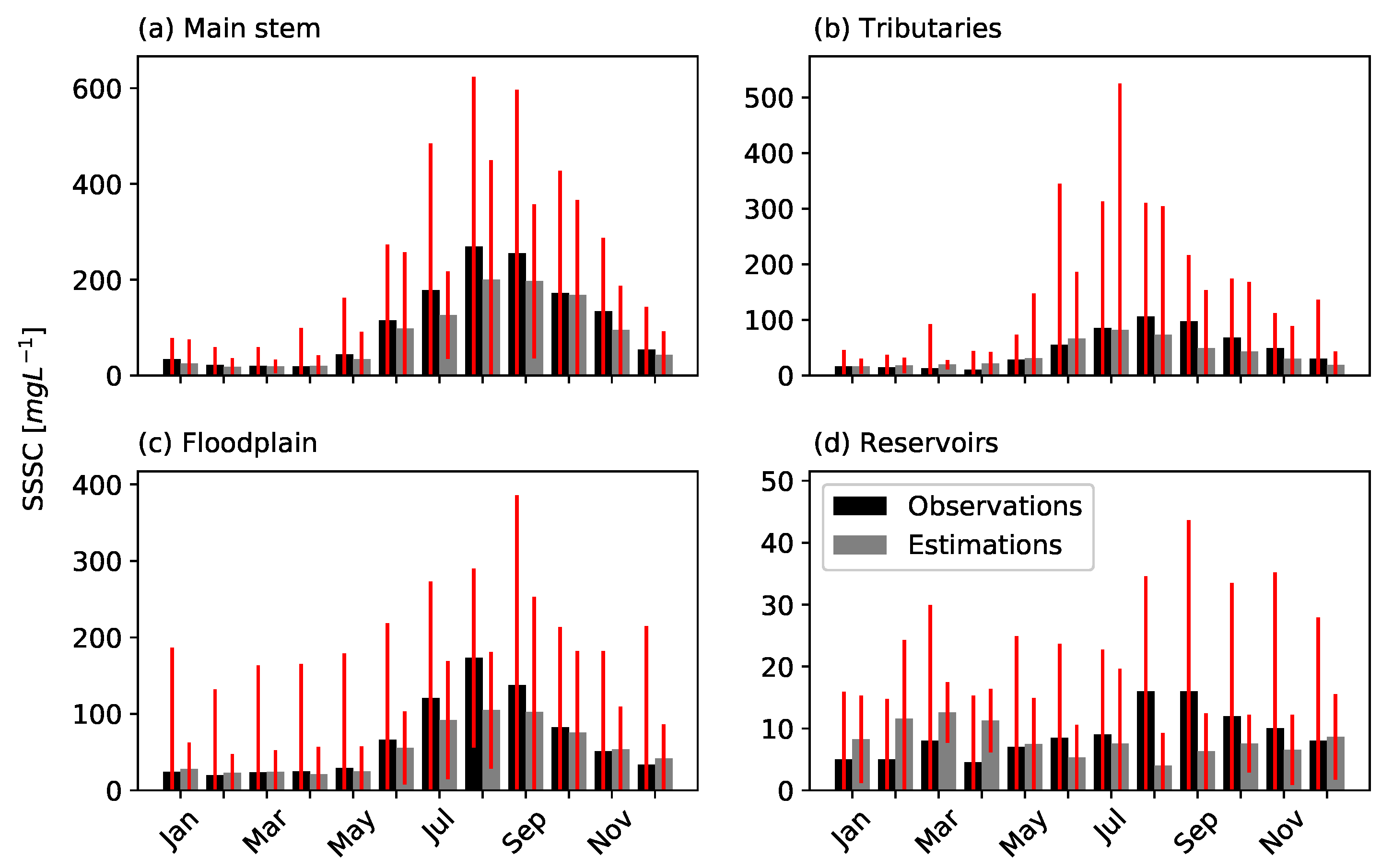
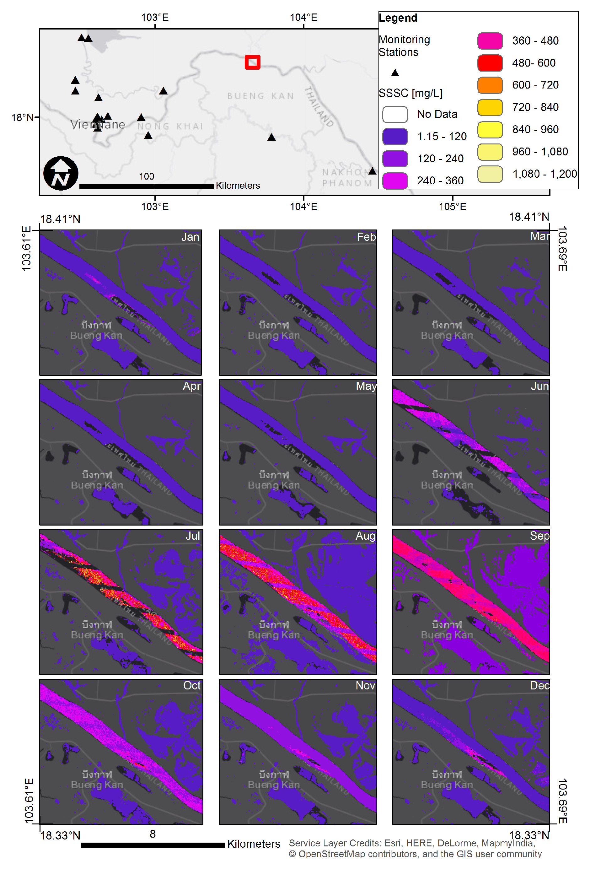
4.1. Improved Spatio-Temporal Resolution and Coverage

Our results are generally consistent with previous work which finds that exponential models using band ratios (as opposed to individual bands) are the most successful at estimating SSSC values over a broad range in concentration [16]. The 19 mg·L${}^{-1}$ RMSE of our model represents an improvement from the previously published models for the Mekong. For example, Suif et al. [34] report an RMSE ranging from 50.2 to 109.7 mg·L${}^{-1}$ for the Mekong main stem, and Wackerman et al. [17] report an RMSE of 34 mg·L${}^{-1}$ for an empirical model of SSCC in the Mekong Delta. Given that these studies were calibrated using fewer in situ observations from a smaller region within the Mekong Basin, our results illustrate that a regionally applicable model can be developed with sufficient in situ observations (n = 118 samples in this study).

The operational model developed in this study considerably increases the availability of SSSC data in the Lower Mekong Basin, making it possible to estimate SSSC for large stretches of the Mekong River and its tributaries. One impact of improved spatial coverage is that cities not located near MRC stations can now monitor SSSC through the web application (Figure 8). For example, MRC currently has water quality stations near the cities of Vientiane, Nong Khai, and Nakhon Phanom along the border of Thailand and Laos, but the city of Bueng Kan, which is located 185 km downstream of the nearest MRC station does not have a source of local water quality data. Through the online tool monthly estimates of SSSC can easily be downloaded for this region. The time series function in the online tool additionally allows users to explore how SSSC may be changing in their region.

In addition to expanding spatial coverage, the model also extends temporal coverage for many parts of the Mekong Basin. For example, SSSC data was collected at the Ban Chai Buri station located at the Songkhram River in Thailand (17.6422 ${}^{\circ }$N, 104.4615 ${}^{\circ }$E) from 2004–2011, but now with remotely sensed SSSC estimates this record is extended to the Landsat series availability (1985-present). Previous efforts to detect changes in sediment concentrations in the Mekong Basin have been difficult in part due to the limited time series of SSSC records at many stations [8,66]. The larger SSSC dataset available through this GEE web application should facilitate future investigations of SSSC trends, allowing users to compare local SSSC estimates for time periods before and after dam construction, major land use changes, or other issues of regional interest.

4.2. Model Limitations

While our model produces a spatially and temporally extensive SSSC dataset, there are limitations to remote sensing models of SSSC that must be carefully considered when analyzing the model results. First, temporal resolution is limited both by satellite repeat cycle, and by cloud cover. Cloud cover during the wet season is particularly problematic because this is when discharge and SSSC is the highest in the Lower Mekong Basin. In our study the calibration dataset includes 52 Landsat overpasses coincident with in situ observation in the wet season, but only 9 of these samples have concentrations over 200 mg·L${}^{-1}$ (Figure 4). As a result, the range of estimated SSSC values produced by the model is smaller than the range of SSSC values in the entire MRC database, and in particular we are missing the highest values during July and August, when in situ measurements of >200 mg·L${}^{-1}$ SSSC are not uncommon. Second, remote sensing techniques measure the optical properties of the top 1–2 meters of the water column, and therefore in shallow water reflectance from the bottom will significantly modify results [67]. We suspect that this is one of the reasons we see the worst match between the MRC dataset and our remotely sensed SSSC dataset for stations downstream of Kratie in the Mekong Floodplain. In this study we attempted to limit interference from the channel bottom by filtering scenes to insure they were at least 60 m from the channel edge. Development of additional filtering algorithms may be required to improve model performance in the region.

Remote Sensing of SSSC concentration can aid regional efforts to assess of water clarity, habitat conditions, nutrient transport and channel morphodynamics, but SSSC estimates cannot be used directly for sediment transport modeling because surface water contains only a fraction of the suspended sediment present over the entire water column. Moreover, the discrepancy between SSSC and depth integrated sediment concentrations will be more significant during the wet season. Particularly at high discharge, bedload transport and course material in the lower water column may constitute a significant fraction of the total sediment load. An additional constraint is that from remote sensing of SSSC alone, it is not possible to differentiate if an increase in SSSC results from mixing of sediment from the lower water column into the upper water column or an increase of suspended sediment in the whole water column. In recognition that depth integrated samples are required for robust sediment transport analysis, the MRC created the Discharge and Sediment Monitoring Program (DSMP) which collected depth integrated samples at 15 locations between 2009 and 2013 through a combination of isokinetic samplers and Acoustic Doppler Current Profilers [68]. Unfortunately, the DSMP dataset is not large enough to calibrate a remote sensing model, but future work could focus on developing rating curves to integrate this information into the model.

4.3. Implications and Future Work

The presented web-application and delivery of SSSC data derived from satellite imagery to users on an operational basis is the first of its kind. With the advent of cloud and web-based applications, such as GEE and Google AppSpot, customizable geospatial data products produced operationally are more widely available. These publicly available applications ultimately allow users greater flexibility to provide input data, filter spatially and temporally, and modify algorithm parameters to provide relevant information for analysis. The web application presented here, along with other such applications (e.g., Robinson et al. [69]), are examples of the changing paradigm from serving static geospatial products to dynamic data products.

There is great potential for this model to be adapted to estimate concentrations of additional water quality constituents, particularly those that are associated with suspended sediments. Future work on this system will focus on utilizing additional sensors, such as Sentinel-2, to improve temporal resolution of satellite observations. Sentinel-2 has been shown to provide high quality estimates of suspended sediments and other water quality parameters [70] and data from Sentinel-2’ has already been successfully integrated with Landsat for monitoring water quality [46]. Furthermore, although remote sensing relies on optically active water constituents, recent studies have explored the utility of remote sensing technologies for optically inactive water quality parameters. For example, Wu et al. [71] used Landsat TM data to empirically estimate total phosphorus concentrations in a riverine environment. The fidelity of such methodologies for estimating other optically inactive water quality parameters, such as nitrogen or pH, has not yet been explored in the Lower Mekong Basin. Expansion of the model and web application to include both optically active and inactive water quality parameters will ultimately provide a more holistic view of water quality and aquatic ecosystem health within the Mekong Basin.

5. Conclusions

The objective of this study was to increase spatial-temporal density of SSSC data in the Lower Mekong Basin by integrating remote sensing observations with in situ measurements. The model developed in this study allows for a consistent and reliable indicator of surface sediment concentrations in an operational near real-time environment. Expanded access to sediment concentration data should be particularly helpful to resource managers interested in the dynamics between sediment concentrations and land use conversions, water policy, and energy production in a globally strategic region.

References

1. Syvitski, J.P.M.; Voosmarty, C.J.; Kettner, A.J.; Green, P. Impact of Humans on the Flux of Terrestrial Sediment to the Global Coastal Ocean. Science 2005, 308, 376–380. [Google Scholar] [CrossRef] [PubMed]
2. Anthony, E.J.; Brunier, G.; Besset, M.; Goichot, M.; Dussouillez, P.; Nguyen, V.L. Linking rapid erosion of the Mekong River delta to human activities. Sci. Rep. 2015, 5, 14745. [Google Scholar] [CrossRef] [PubMed] [Green Version]
3. Mekong River Commission. State of the Basin Report: 2005; Mekong River Commission: Phnom Penh, Cambodia, 2005. [Google Scholar]
4. Milliman, J.; Syvitski, J.P.M. Geomorphic/Tectonic Control of Sediment Discharge to the Ocean: The Importance of Small Mountainous Rivers. J. Geol. 1992, 100, 525–544. [Google Scholar] [CrossRef]
5. Kondolf, G.M.; Rubin, Z.K.; Minear, J.T. Dams on the Mekong: Cumulative sediment starvation. Water Resour. Res. 2014, 50. [Google Scholar] [CrossRef]
6. Kummu, M.; Varis, O. Sediment-related impacts due to upstream reservoir trapping, the Lower Mekong River. Geomorphology 2007, 85, 275–293. [Google Scholar] [CrossRef]
7. Kummu, M.; Lu, X.; Wang, J.J.; Varis, O. Basin-wide sediment trapping efficiency of emerging reservoirs along the Mekong. Geomorphology 2010, 119, 181–197. [Google Scholar] [CrossRef]
8. Walling, D.E. The Changing Sediment Load of the Mekong River. Ambio 2008, 37, 150–157. [Google Scholar] [CrossRef]
9. Mekong River Commission. State of the Basin Report: 2010; Mekong River Commission: Phnom Penh, Cambodia, 2010. [Google Scholar]
10. Ritchie, J.C.; Zimba, P.V.; Everitt, J.H. Remote Sensing Techniques to Assess Water Quality. Photogramm. Eng. Remote Sens. 2003, 69, 695–704. [Google Scholar] [CrossRef]
11. Wang, F.; Han, L.; Kung, H.T.; van Arsdale, R. Applications of Landsat-5 TM imagery in assessing and mapping water quality in Reelfoot Lake, Tennessee. Int. J. Remote Sens. 2006, 27, 5269–5283. [Google Scholar] [CrossRef]
12. Park, E.; Latrubesse, E.M. Modeling suspended sediment distribution patterns of the Amazon River using MODIS data. Remote Sens. Environ. 2014, 147, 232–242. [Google Scholar] [CrossRef]
13. Umar, M.; Rhoads, B.L.; Greenberg, J.A. Use of multispectral satellite remote sensing to assess mixing of suspended sediment downstream of large river confluences. J. Hydrol. 2018, 556, 325–338. [Google Scholar] [CrossRef]
14. Myint, S.W.; Walker, N.D. Quantification of surface suspended sediments along a river dominated coast with NOAA AVHRR and Sea WiFS measurements: Louisiana, USA. Int. J. Remote Sens. 2002, 23, 3229–3249. [Google Scholar] [CrossRef]
15. Matthews, M.W. A current review of empirical procedures of remote sensing in Inland and near-coastal transitional waters. Int. J. Remote Sens. 2011, 32, 6855–6899. [Google Scholar] [CrossRef]
16. Long, C.M.; Pavelsky, T.M. Remote sensing of suspended sediment concentration and hydrologic connectivity in a complex wetland environment. Remote Sens. Environ. 2013, 129, 197–209. [Google Scholar] [CrossRef]
17. Wackerman, C.; Hayden, A.; Jonik, J. Deriving spatial and temporal context for point measurements of suspended-sediment concentration using remote-sensing imagery in the Mekong Delta. Cont. Shelf Res. 2017, 147, 231–245. [Google Scholar] [CrossRef]
18. Dekker, A.; Vos, R.; Peters, S. Comparison of remote sensing data, model results and in situ data for total suspended matter (TSM) in the southern Frisian lakes. Sci. Total Environ. 2001, 268, 197–214. [Google Scholar] [CrossRef]
19. Laanen, M.L. Yellow Matters: Improving the Remote Sensing of Coloured Dissolved Organic Matter in Inland Freshwaters; Water Insight B.V.: Wageningen, The Netherlands, 2007. [Google Scholar]
20. Tilstone, G.H.; Peters, S.W.; van der Woerd, H.J.; Eleveld, M.A.; Ruddick, K.; Schönfeld, W.; Krasemann, H.; Martinez-Vicente, V.; Blondeau-Patissier, D.; Röttgers, R.; et al. Variability in specific-absorption properties and their use in a semi-analytical ocean colour algorithm for MERIS in North Sea and Western English Channel Coastal Waters. Remote Sens. Environ. 2012, 118, 320–338. [Google Scholar] [CrossRef] [Green Version]
21. Cox, R.M.; Forsythe, R.D.; Vaughan, G.E.; Olmsted, L. Assessing water quality in Catawba River reservoirs using Landsat Thematic Mapper satellite data. Lake Reserv. Manag. 1998, 14, 405–416. [Google Scholar] [CrossRef]
22. Dekker, A.G.; Vos, R.; Peters, S. Analytical algorithms for lake water TSM estimation for retrospective analyses of TM and SPOT sensor data. Int. J. Remote Sens. 2002, 23, 15–35. [Google Scholar] [CrossRef]
23. Brezonik, P.; Menken, K.D.; Bauer, M. Landsat-based remote sensing of lake water quality characteristics, including chlorophyll and colored dissolved organic matter (CDOM). Lake Reserv. Manag. 2005, 21, 373–382. [Google Scholar] [CrossRef]
24. Curran, P.; Hansom, J.; Plummer, S.; Pedley, M. Multispectral remote sensing of nearshore suspended sediments: A pilot study. Int. J. Remote Sens. 1987, 8, 103–112. [Google Scholar] [CrossRef]
25. Novo, E.; Hansom, J.; Curran, P. The effect of viewing geometry and wavelength on the relationship between reflectance and suspended sediment concentration. Int. J. Remote Sens. 1989, 10, 1357–1372. [Google Scholar] [CrossRef] [Green Version]
26. Hellweger, F.; Schlosser, P.; Lall, U.; Weissel, J. Use of satellite imagery for water quality studies in New York Harbor. Estuar. Coast. Shelf Sci. 2004, 61, 437–448. [Google Scholar] [CrossRef]
27. Fleifle, A. Suspended Sediment Load Monitoring Along the Mekong River from Satellite Images. J. Earth Sci. Clim. Chang. 2013, 4. [Google Scholar] [CrossRef]
28. Papoutsa, C.; Retalis, A.; Toulios, L.; Hadjimitsis, D. Defining the Landsat TM/ETM+ and chris/proba spectral regions in which turbidity can be retrieved in inland water bodies using eld spectroscopy. Int. J. Remote Sens. 2014, 35, 1674–1692. [Google Scholar] [CrossRef]
29. Overeem, I.; Hudson, B.D.; Syvitski, J.P.M.; Mikkelsen, A.B.; Hasholt, B.; van den Broeke, M.R.; Noël, B.P.Y.; Morlighem, M. Substantial export of suspended sediment to the global oceans from glacial erosion in Greenland. Nat. Geosci. 2017, 10, 859. [Google Scholar] [CrossRef]
30. Nechad, B.; Ruddick, K.; Park, Y. Calibration and validation of a generic multisensor algorithm for mapping of total suspended matter in turbid waters. Remote Sens. Environ. 2010, 110, 854–866. [Google Scholar] [CrossRef]
31. Feng, L.; Hu, C.; Chen, X.; Song, Q. Influence of the Three Gorges Dam on total suspended matters in the Yangtze Estuary and its adjacent coastal waters: Observations from MODIS. Remote Sens. Environ. 2014, 140, 779–788. [Google Scholar] [CrossRef]
32. Gholizadeh, M.H.; Melesse, A.M.; Reddi, L. A Comprehensive Review on Water Quality Parameters Estimation Using Remote Sensing Techniques. Sensors 2016, 16, 1298. [Google Scholar] [CrossRef] [PubMed]
33. Bowers, D.; Binding, C. The optical properties of mineral suspended particles: A review and synthesis. Estuar. Coast. Shelf Sci. 2006, 67, 219–230. [Google Scholar] [CrossRef]
34. Suif, Z.; Fleifle, A.; Yoshimura, C.; Saavedra, O. Spatio-temporal patterns of soil erosion and suspended sediment dynamics in the Mekong River Basin. Sci. Total Environ. 2016, 568, 933–945. [Google Scholar] [CrossRef] [PubMed]
35. Dang, T.D.; Cochrane, T.A.; Arias, M.E. Quantifying sediment dynamics in mega deltas using remote sensing data: A case study of the Mekong floodplains. Int. J. Appl. Earth Obs. 2018, 68, 105–115. [Google Scholar] [CrossRef]
36. Bui, Y.T.; Orange, D.; Visser, S.M.; Hoanh, C.T.; Laissus, M.; Poortinga, A.; Tran, D.T.; Stroosnijder, L. Lumped surface and sub-surface runoff for erosion modeling within a small hilly watershed in northern Vietnam. Hydrol. Process. 2014, 28, 2961–2974. [Google Scholar] [CrossRef]
37. Gorelick, N.; Hancher, M.; Dixon, M.; Ilyushchenko, S.; Thau, D.; Moore, R. Google Earth Engine: Planetary-scale geospatial analysis for everyone. Remote Sens. Environ. 2017, 202, 18–27. [Google Scholar] [CrossRef]
38. Mekong River Commission. Hydrological/Water Quality Database; Mekong River Commission: Phnom Penh, Cambodia, 2011. [Google Scholar]
39. Pekel, J.F.; Cottem, A.; Gorelick, N.; Belward, A.S. High-resolution mapping of global surface water and its long-term changes. Nature 2016, 540, 418–422. [Google Scholar] [CrossRef] [PubMed]
40. Chander, G.; Markham, L.; Halder, D.L. Summary of current radiometric calibration coefficients for Landsat MSS, TM, ETM+, and EO-1 ALI sensors. Remote Sens. Environ. 2009, 113, 893–903. [Google Scholar] [CrossRef] [Green Version]
41. Dash, P.; Walker, N.; adn Eurico D’Sa, D.M.; Ladner, S. Atmospheric Correction and Vicarious Calibration of Oceansat-1 Ocean Color Monitor (OCM) Data in Coastal Case 2 Waters. Remote Sens. 2012, 4, 1716–1740. [Google Scholar] [CrossRef] [Green Version]
42. Tian, L.; Wai, O.W.H.; Chen, X.; Liu, Y.; Feng, L.; Li, J.; Huang, J. Assessment of Total Suspended Sediment Distribution under Varying Tidal Conditions in Deep Bay: Initial Results from HJ-1A/1B Satellite CCD Images. Remote Sens. 2014, 6, 9911–9929. [Google Scholar] [CrossRef] [Green Version]
43. Barrett, D.C.; Frazier, A.E. Automated Method for Monitoring Water Quality Using Landsat Imagery. Water 2016, 8, 257. [Google Scholar] [CrossRef]
44. Liu, H.; Li, Q.; Shi, T.; Hu, S.; Wu, G.; Zhou, Q. Application of Sentinel 2 MSI Images to Retrieve Suspended Particulate Matter Concentrations in Poyang Lake. Remote Sens. 2017, 9, 761. [Google Scholar] [CrossRef]
45. Carswell, T.; Costa, M.; Young, E.; Komick, N.; Gower, J.; Sweeting, R. Evaluation of MODIS-Aqua Atmospheric Correction and Chlorophyll Products of Western North American Coastal Waters Based on 13 Years of Data. Remote Sens. 2017, 9, 1063. [Google Scholar] [CrossRef]
46. Page, B.P.; Kumar, A.; Mishra, D.R. A novel cross-satellite based assessment of the spatio-temporal development of a cyanobacterial harmful algal bloom. Int. J. Appl. Earth Obs. 2018, 66, 69–81. [Google Scholar] [CrossRef]
47. Watanabe, F.S.Y.; Alcântara, E.; Rodrigues, T.W.P.; Imai, N.N.; Barbosa, C.C.F.; da Silva Rotta, L.H. Estimation of Chlorophyll-a Concentration and the Trophic State of the Barra Bonita Hydroelectric Reservoir Using OLI/Landsat-8 Images. Int. J. Environ. Res. Public Health 2015, 12, 10391–10417. [Google Scholar] [CrossRef] [PubMed] [Green Version]
48. Rotta, L.H.; Alcântara, E.H.; Watanabe, F.S.; Rodrigues, T.W.; Imai, N.N. Atmospheric correction assessment of SPOT-6 image and its influence on models to estimate water column transparency in tropical reservoir. Remote Sensing Applications: Society and Environment 2016, 4, 158–166. [Google Scholar] [CrossRef]
49. Pahlevan, N.; Schott, J.R.; Franz, B.A.; Zibordi, G.; Markham, B.; Bailey, S.; Schaaf, C.B.; Ondrusek, M.; Greb, S.; Strait, C.M. Landsat 8 remote sensing reflectance (Rrs) products: Evaluations, intercomparisons, and enhancements. Remote Sens. of Environ. 2017, 190, 289–301. [Google Scholar] [CrossRef]
50. Masek, J.G.; Vermote, E.F.; Saleous, N.; Wolfe, R.; Hall, F.G.; Huemmrich, F.; Gao, F.; Kutler, J.; Lim, T.K. A Landsat surface reflectance data set for North America, 1990-2000. IEEE Geosci. Remote Sci. 2006, 3, 68–72. [Google Scholar] [CrossRef]
51. Vermote, E.F.; Saleous, N.; Justice, C.O.; Kaufman, Y.J.; Privette, J.L.; Remer, L.; Roger, J.C.; Tanre, D. Atmospheric correction of visible to middle-infrared EOS-MODIS data over land surfaces: Background, operational algorithm, and validation. J. Geophys. Res. 1997, 102, 17131–17141. [Google Scholar] [CrossRef]
52. Vermote, E.F.; Saleous, N.; Justice, C.O. Atmospheric correction of MODIS data in the visible to middle infrared: First results. Remote Sens. Environ. 2002, 83, 97–111. [Google Scholar] [CrossRef]
53. Vermote, E.F.; Tanre, D.; Deuze, J.L.; Herman, M.; Morcrette, J.J. Second Simulation of the Satellite Signal in the Solar Spectrum, 6S: An Overview. IEEE Trans. Geosci. Remote Sens. 1997, 35, 675–686. [Google Scholar] [CrossRef]
54. Kotchenova, S.Y.; Vermote, E.F.; Mataresse, R.; Frank, J.K., Jr. Validation of a vector version of the 6S radiative transfer code for atmospheric correction of satellite data. Part I: Path Radiance. Appl. Opt. 2006, 45, 6726–6774. [Google Scholar] [CrossRef]
55. Kotchenova, S.Y.; Vermote, E.F. Validation of a vector version of the 6S radiative transfer code for atmospheric correction of satellite data. Part II: Homogeneous Lambertian and anisotropic surfaces. Appl. Opt. 2007, 46, 4455–4464. [Google Scholar] [CrossRef] [PubMed]
56. Potes, M.; Costa1, M.J.; Salgado, R. Satellite remote sensing of water turbidity in Alqueva reservoir and implications on lake modelling. Hydrol. Earth Syst. Sci. 2012, 16, 1623–1633. [Google Scholar] [CrossRef] [Green Version]
57. Giardino, C.; Bresciani, M.; Cazzaniga, I.; Schenk, K.; Rieger, P.; Braga, F.; Matta, E.; Brando, V.E. Evaluation of Multi-Resolution Satellite Sensors for Assessing Water Quality and Bottom Depth of Lake Garda. Sensors 2014, 14, 24116–24131. [Google Scholar] [CrossRef] [PubMed] [Green Version]
58. Shang, P.; Shen, F. Atmospheric Correction of Satellite GF-1/WFV Imagery and Quantitative Estimation of Suspended Particulate Matter in the Yangtze Estuary. Sensors 2016, 16, 1997. [Google Scholar] [CrossRef] [PubMed]
59. Foga, S.; Scaramuzza, P.L.; Guo, S.; Zhu, Z.; Dilley, R.D.; Beckmann, T.; Schmidt, G.L.; Dwyer, J.L.; Hughes, M.J.; Laue, B. Cloud detection algorithm comparison and validation for operational Landsat data products. Remote Sens. Environ. 2017, 194, 379–390. [Google Scholar] [CrossRef] [Green Version]
60. Zhu, Z.; Wang, S.; Woodcock, C.E. Improvement and expansion of the Fmask algorithm: cloud, cloud shadow, and snow detection for Landsats 4–7, 8, and Sentinel 2 images. Remote Sens. Environ. 2015, 159, 269–277. [Google Scholar] [CrossRef]
61. Oliphant, T.E. Python for Scientific Computing. Comput. Sci. Eng. 2007, 9, 10–20. [Google Scholar] [CrossRef] [Green Version]
62. Millman, K.J.; Aivazis, M. Python for Scientists and Engineers. Comput. Sci. Eng. 2011, 13, 9–12. [Google Scholar] [CrossRef] [Green Version]
63. Poortinga, A.; Clinton, N.; Saah, D.; Cutter, P.; Chishtie, F.; Markert, K.N.; Anderson, E.R.; Troy, A.; Fenn, M.; Tran, L.H.; Bean, B.; Nguyen, Q.; Bhandari, B.; Johnson, G.; Towashiraporn, P. An operational Before-After-Control-Impact (BACI) designed platform for vegetation monitoring at planetary scale. Remote Sens. 2018, 10, 760. [Google Scholar] [CrossRef]
64. Moriasi, D.N.; Arnold, J.G.; Van Liew, M.W.; Bingner, R.L.; Harmel, R.D.; Veith, T.L. Model evaluation guidelines for systematic quantification of accuracy in watershed simulations. Trans. ASABE 2007, 50, 885–900. [Google Scholar] [CrossRef]
65. McCain, C.; Hooker, S.; Feldman, G.; Bontempi, P. Satellite data for ocean biology, biogeochemistry, and climate research. Eos Trans. Am. Geophys. Union 2006, 87, 337–343. [Google Scholar] [CrossRef]
66. Wang, J.; Lu, X.X.; Kummu, M. Sediment load estimates and variations in the Lower Mekong River. River Res. Appl. 2011, 27, 33–46. [Google Scholar] [CrossRef]
67. Volpe, V.; Silvestri, S.; Marani, M. Remote sensing retrieval of suspended sediment concentration in shallow waters. Remote Sens. Environ. 2011, 115, 44–54. [Google Scholar] [CrossRef]
68. Koehnken, L. Discharge Sediment Monitoring Project (DSMP) 2009–2013 Summary and Analysis of Results: Final Report; Mekong River Commission: Vientiane, Lao PDR, 2014. [Google Scholar]
69. Robinson, N.P.; Allred, B.W.; Jones, M.W.; Moreno, A.; Kimball, J.S.; Naugle, D.E.; Erikson, T.A.; Richardson, A.D. A Dynamic Landsat Derived Normalized Difference Vegetation Index (NDVI) Product for the Conterminous United States. Remote Sens. 2017, 9, 863. [Google Scholar] [CrossRef]
70. Toming, K.; Kutser, T.; Laas, A.; Sepp, M.; Paavel, B.; Noges, T. First Experiences in Mapping Lake Water Quality Parameters with Sentinel-2 MSI Imagery. Remote Sens. 2016, 8. [Google Scholar] [CrossRef]
71. Wu, C.; Wu, J.; Qi, J.; Zhang, L.; Huang, H.; Lou, L.; Chen, Y. Empirical estimation of total phosphorus concentration in the mainstream of the Qiantang River in China using Landsat TM data. Remote Sens. Environ. 2010, 31, 2309–2324. [Google Scholar] [CrossRef] [Green Version]
Figure 1. Study area map of the Lower Mekong Basin highlighting geopolitical boundaries, the river systems in the region, and the water quality monitoring stations included in the MRC water quality database.
Remotesensing 10 00909 g001
Figure 2. General workflow schematic for building SSSC empirical model from satellite imagery.
Remotesensing 10 00909 g002
Figure 3. The infrastructure for spatial application development provided by Google. GEE consists of a cloud-based data catalogue and computing platform. The App Engine framework was used to serve the data to a web browser and communicate with the GEE using the Python API. Figure reused with permission from Poortiga et al. [63].
Remotesensing 10 00909 g003
Figure 4. (a) Map highlighting the locations of water quality stations included in the calibration and validation dataset. Stations are coded by number of coincident Landsat 4, 5 and 7 observations from 1985 to 2011 for each station. Unused stations left out due to bank proximity or lack of coincidence Landsat data are shown in white; (b) Temporal distribution of Landsat observations coincident with in situ SSSC measurements in the calibration dataset (n = 189); (c) Distribution of in situ SSSC values in the calibration dataset.
Remotesensing 10 00909 g004
Figure 5. Model calibration using the ρ R e d ρ G r e e n band ratio with a exponential fit from Equation (1) (a) and validation (b,c) plots of statistical modeling for the dry (b) and wet (c) seasons.
Remotesensing 10 00909 g005
Figure 6. Monthly median estimates of SSSC from 1985–2011 against observed monthly median SCC for the 44 water quality stations used in this study. The stations were classified into four groups: (a) mainstem of Mekong river; (b) tributary river systems; (c) the Mekong floodplain region and (d) reservoirs. Red bars indicate the standard deviation of each month from all stations in the group.
Remotesensing 10 00909 g006
Figure 7. A screenshot of the Mekong Suspended Sediment Monitoring web application (https://mekong-ssc.appspot.com). To download a dataset, users set their desired parameters in the right panel. The region of interest can be a polygon drawn directly on the map. A mean composite for the time period is processed on the fly and is available for users to download directly.
Remotesensing 10 00909 g007
Figure 8. Estimated monthly average SSSC from 1985–2011 near Bueng Kan city located 185 km downstream of the nearest MRC station. Top map displays northeast Thailand bordering Laos with surrounding MRC water quality monitoring stations and an indication of the monthly SSSC maps. The SSSC scale in the legend refers to the monthly maps below.
Remotesensing 10 00909 g008