A Ship Detector Applying Principal Component Analysis to the Polarimetric Notch Filter

Abstract

Ship detection using polarimetric synthetic aperture radar (PolSAR) data has attracted a lot of attention in recent years. Polarimetry can provide information regarding the scattering mechanisms of targets, which helps discriminate between ships and sea clutter. This enhancement is particularly valuable when we aim at detecting smaller vessels in rough sea states. This work exploits a ship detector called the Geometrical Perturbation-Polarimetric Notch Filter (GP-PNF), and it is aimed at improving its performance especially when less polarimetric images are available (e.g., dual-polarimetric data). The idea is to design a new polarimetric feature vector containing more features that are renowned to allow separation between ships and sea clutter. Then, a Principal Component Analysis (PCA) is further used to reduce the dimensionality of the new feature space. Experiments on four real Sentinel-1 datasets are carried out to demonstrate the validity of the proposed method and compare it against other ship detectors. Analyses of the experimental results show that the proposed algorithm can not only reduce the false alarms significantly, but also enhance the target-to-clutter ratio (TCR) so that it can more effectively detect weaker ships.

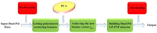
1. Introduction

Over the past several decades, maritime surveillance has been given a high priority in many countries. Besides Automatic Identification System (AIS) [1], synthetic aperture radar (SAR) has been widely used in maritime surveillance due to its ability to image at day-and-night and the capability to penetrate clouds. However, ship detection is still a challenging task especially when we want to detect smaller vessels or when the sea state is high. The ocean backscattering caused by surface wind or other oceanographic phenomena can also generate many false alarms. On the other hand, the backscattering from ships, is mainly composed of multiple reflections on the hull and metallic structures and it can be relatively weak for smaller vessels [2]. Hence, powerful methodologies, that are able to effectively remove false alarms and simultaneously detect weaker ships play an important role in SAR ship detection.

Up to now, much work has been done on ship detection, exploiting different airborne and spaceborne SAR systems such as AIRSAR, TerraSAR-X and Radarsat-2 [3]. In earlier studies, most methods explored single polarized SAR images, in which Constant False Alarm Rate (CFAR) detection was largely used [4,5]. Eldhuset [6] adopted an adaptive filter to detect ship candidates, and further took advantage of the ship wake as a secondary indicator. This could supply additional information for reducing the number of false alarms. Leng et al. [7] combined the intensity distribution and the spatial distribution of the single-channel SAR image for reducing the false alarms and detecting ships. Based on the discrete wavelet transform, Tello et al. [8] proposed a new detector for ship detection by multiplying four different subbands. Although traditional single-channel data can be useful for detecting larger ships in relatively calm sea conditions, using them to detect smaller ships in higher sea states is still challenging.

Compared with the single polarized mode, a fully polarized mode can obtain more backscattering information, and therefore can improve the discrimination between targets and sea clutter. In recent years, many algorithms using quad-polarimetric SAR (PolSAR) data have been developed. The most straightforward approaches directly utilize the PolSAR data as the underlying features for ship detection using the covariance/coherency matrix. Apart from the polarimetric SPAN (total power) detector [9], the Polarimetric Whitening Filter (PWF) detector [10] is the most-used algorithm for ship detection. It uses all the channels to reduce optimally the speckle [11] providing better performance than SPAN. However, the PWF detector may miss weaker vessels [10].

Some of the algorithms exploit statistics. On the basis of full polarimetric SAR data, Liu et al. [12] applied the CFAR detector using Gaussian distribution to each band. The final results relied on the highest probability of detection among all the three independent channels. New models have been proposed and they show better performance. These statistical models include Weibull, Gamma, $G^0$, and K distribution.

Alternatively, different polarimetric decomposition (PD) methods or parameters can be calculated from the covariance or coherency matrix. Some of these parameters can be used to discriminate between vessels and sea clutter. Sugimoto et al. utilized Yamaguchi decomposition to find the difference between ships and sea surface [13]. Wang et al. [14] employed different PD algorithms to analyze the scattering of several types of ships. In [15], the Symmetric Scattering Characterization Method (SSCM), an extension of Cameron’s method [16], was used for ship detection. Preliminary results, which were tested on the C-Band AIRSAR data, demonstrated the soundness of the approach. Cloude et al. [17] utilized the entropy and $\alpha$ angle that calculated from the Cloude–Pottier decomposition to detect targets successfully. Nunziata et al. [18] exploited the reflection symmetry (RF) characteristic of the sea clutter to detect targets at sea. With the aim of finding a more robust algorithm, Yang et al. [19] developed a new parameter to reflect the similarity degree between two scattering matrices, and introduced a general contrast optimization method that can effectively enhance the Target-to-Clutter Ratio (TCR) for ships [20]. Marino et al. [21] proposed a new detector for object detection by using the Huynen fork, which extracted the target features in the polarimetric target complex space. This culminated in a ship detector called the Geometrical Perturbation-Polarimetric Notch Filter (GP-PNF) by Marino et al. [22].

On the whole, all the aforementioned methods mainly belong to the “pixel based” category, which means most of the features are extracted with a pixel approach, using single-look scatter matrices or multilook covariance/coherency matrices [23]. Some researchers widened this concept considering the surrounding polarimetric information around the target pixels. Wang et al. [23] adopted superpixel models to derive new polarimetric scattering features for ship detection. Zhang et al. [24,25] used the difference between the ship pixels and their surrounding clutter pixels to improve TCR for ship detection. However, this algorithm is still time-consuming because of the burden of calculating the polarimetric covariance difference matrix (PCDM) and eigenvalues.

With today’s technology, quad-polarimetric SAR data is only available with limited swath widths [26]. Thus, using SAR data with dual polarization and wider swaths is more practical for operational purposes [26].

In this work, we take advantage of the freely available European Space Agency (ESA) Sentinel-1 data. Sentinel-1 was launched by ESA in April 2014. It has several modes of operation and can achieve medium-to-high-resolution imaging with wide coverage [27]. The interferometric wide swath (IWS) mode acquires VH/VV (or HH/HV) dual-polarization combinations and can provide 250-km swath at 5 m × 20 m (range × azimuth) spatial resolution in single look complex format. Several works have used Sentinel-1 for ship detection [28,29,30], demonstrating that Sentinel-1 data is well-suited for this task. However, dual-polarization SAR can have problems detecting weaker vessels, especially when the sea state is higher.

In recent years, principle component analysis (PCA) [31] has been largely used within remote sensing techniques [32]. Ready et al. [33] demonstrated that significant improvements in Signal to Noise Ratio (SNR) could be achieved from noisy multi-spectral data using PCA. Eklundh [34] et al. found that, using the standardized principal components analysis (sPCA), we could more effectively improve SNR than the unstandardized principal components analysis (uPCA). Lee et al. [35] used the principal components transform (PCT) for speckle reduction in PolSAR images.

Encouraged by the aforementioned methods, this paper proposes an improved GP-PNF method for enhancing the TCR values of ships, especially for weaker scattering ships in rough sea conditions. Four real Sentinel-1 IW datasets are further used to test its performance.

The rest of the paper is structured as follows. The theoretical background is introduced in Section 2. Section 3 presents the proposed scheme of ship detection based on GP-PNF and PCA. In Section 4, the experimental results and discussions on the Sentinel-1 data, which consists of a harbor dataset with calm sea state, a harbor dataset with moderate/rough sea state and two offshore datasets with rough sea state, are presented in detail. Finally, Section 5 concludes the paper.

2. Theoretical Background

2.1. Theory of Polarimetric SAR Data

Polarimetric information of objects can be effectively represented by the scattering matrix [S]. Taking a linear horizontal and vertical polarization basis for example, [S] can be expressed as [36]:

$$\begin{array}{cc}\hfill [S]& =\left[\begin{array}{cc}{S}_{HH}& S_{HV}\\ S_{VH}& S_{VV}\end{array}\right],\hfill \end{array}$$

(1)

where, for instance, $S_{HV}$ denotes the horizontal receiving and vertical transmitting polarization channel. When a target is reciprocal, its [S] scattering matrix is symmetrical, that is, $S_{HV}$ = $S_{VH}$ except for thermal noise. For the dual-pol case, the scattering matrix [S] can be simplified as a column vector [37]:

$$\begin{array}{cc}\hfill \underline{k}{}_{dual-pol}& ={[k_{d1},k_{d2}]}^T\hfill \end{array}$$

(2)

where $\underline{k}{}_{dual-pol}$ stands for the scattering vector of dual-pol SAR [38], and the superscript “T” denotes the matrix transpose. The elements $k_{d1}$ and $k_{d2}$ respectively indicate the co-polar scattering element ($S_{HH}$ or $S_{VV}$) and the cross-polar scattering element ($S_{HV}$ or $S_{VH}$).

To further analyze the physical information of distributed targets, we can use the second-order statistics of the scattering vector, such as the covariance matrix [C] or the coherence matrix [T]. In this paper, we choose VH/VV as the dual polarimetric mode. Therefore, the resulting covariance matrix is defined as [36]:

$$\begin{array}{cc}\hfill \left[\begin{array}{c}{C}_{dual-pol}\end{array}\right]& =〈{\underline{k}}_{dual-pol}·{\underline{k}}_{dual-pol}^H〉=\left[\begin{array}{cc}\langle |S_{VV}^2|\rangle & \langle |S_{VV}{S}_{VH}^{\ast }|\rangle \\ \langle |S_{VV}^{\ast }{S}_{VH}|\rangle & \langle |S_{VH}^2|\rangle \end{array}\right]\hfill \\ & =\left[\begin{array}{cc}{C}_{11}& C_{12}\\ C_{21}& C_{22}\end{array}\right],\hfill \end{array}$$

(3)

where the superscript “H” represents the conjugate transpose, $\langle ·\rangle$ indicates spatial averaging, $|·|$ is the magnitude, and “*” denotes the complex conjugate.

2.2. Geometrical Perturbation-Polarimetric Notch Filter (GP-PNF)

GP-PNF is proposed by Marino et al. [38] and it is an adaptation of the Geometrical Perturbation Filter (GPF) [39] to work as a notch filter in the polarimetric space. GP-PNF can effectively detect objects on the sea by isolating and rejecting the sea return in the polarimetric space of the covariance matrices.

In GP-PNF, a 6D partial scattering feature vector $\underline{t}$ is firstly constructed, i.e., [40]:

$$\begin{array}{cc}\hfill \underline{t}& =\mathrm{Trace}([C_{quad-pol}]{\mathsf{\Psi }}_q)={[t_1,t_2,t_3,t_4,t_5,t_6]}^T\hfill \\ & =[\langle |k_1{|}^2\rangle ,\langle |k_2{|}^2\rangle ,\langle |k_3{|}^2{\rangle ,\langle k_1^{\ast }{k}_2\rangle ,\langle k_1^{\ast }{k}_3\rangle ,\langle k_2^{\ast }{k}_3\rangle ]}^T,\hfill \end{array}$$

(4)

where ${\mathsf{\Psi }}_q$ is a complete set of 6×6 basis matrices under a Hermitian inner product and $k_i$ (i = 1, 2, 3) are the elements of the scattering vector $\underline{k}$ derived from the Sinclair scattering matrix [S] in the case of monostatic sensor and reciprocity. Considering we will use dual-pol data in this work, the dual polarimetric feature vector ${\underline{t}}_{dual-pol}$ is exploited [39]:

$$\begin{array}{cc}\hfill {\underline{t}}_{dual-pol}& =\mathrm{Trace}([C_{dual-pol}]{\mathsf{\Psi }}_d)\hfill \\ & =[\langle |k_{d1}{|}^2\rangle ,\langle |k_{d2}{|}^2{\rangle ,\langle k_{d1}^{\ast }{k}_{d2}\rangle ]}^T.\hfill \end{array}$$

(5)

Please note that the dual-pol feature vector can only provide an incomplete observation of the full polarimetric space [40].

Then, a vector ${\underline{t}}_T$ is further designed to represent the partial target. Moreover, a pseudo target ${\underline{t}}_P$ is also obtained perturbing ${\underline{t}}_T$ slightly (i.e., all the components of ${\underline{t}}_T$ are modified slightly). Thus, after a series of mathematical manipulations [40], the final dual polarimetric detector is defined as:

$$\gamma =\frac{1}{\sqrt{1+RedR\frac{P_C}{P_T}}},$$

(6)

where $RedR$ is a parameter called Reduction Ratio, $P_C$ and $P_T$ represent the power of clutter and target, respectively.

In summary, if the partial target has a strong component on the target of interest, $P_T$ will be bigger than $P_C$ and $\gamma$ will be closer to 1.

2.3. Principal Component Analysis (PCA)

Rich multidimensional datasets often allow for extracting many features. In the case of radar polarimetric data, we can extract the so called “polarimetric features”. However, some of these features will be correlated. Thus, it would be helpful to reduce the number of features but still retain the useful information in the original datasets [31]. Principal Component Analysis (PCA) is an effective tool to reduce the dimensions of features [41]. Its goal is to find a subspace, where most of the variance in the previous feature space is contained [42].

Suppose that our signal X is composed of n measurements of a vector $\underline{x}$ as n random variables, and we want to reduce the dimension from n to m, where m is smaller than n. Firstly, we let the signal X have the covariance matrix [$\mathsf{\Sigma }$] with respectively [P] and [$\mathsf{\Lambda }$] eigenvector and eigenvalue matrices, that is [43]:

$$[\mathsf{\Lambda }]={[P]}^T[\mathsf{\Sigma }][P].$$

(7)

It can be proven that the set of m ($m\le n$) eigenvectors (here, called ${\underline{A}}_m$) of $[\sum ]$, which corresponds to the m largest eigenvalues, would minimize the mean square reconstruction error compared to all the other possible choices of m orthonormal basis vectors [43]. Then, the PCA signal $\underline{Y}$ can be given as:

$$\underline{Y}=[X]{\underline{A}}_m,$$

(8)

where [X] is the original data matrix and ${\underline{A}}_m$ = [$a_1,a_2,\dots ,a_m$]${}^T$.

3. Methodology

The first part of this section analyzes some polarimetric features used in the proposed method. In the second part, the new polarimetric scattering vectors will be created. At last, we will use the framework of GP-PNF to design the ship detector.

3.1. Analysis of Polarimetric Features

Polarimetric features can be divided into two categories: (1) selected directly from the PolSAR data such as the scattering matrix [S] and the covariance matrix [C]; (2) selected after manipulations of the elements of the scattering or covariance matrix.

The overall intensity is a very important feature in ship detection. It is calculated as the sum of the diagonal elements of the covariance matrix [$C_{dual-pol}$] [9]:

$$SPAN=C_{11}+C_{22}.$$

(9)

Ocean backscattering in the cross-polarization channel is generally weaker than in the co-polarization channel. This is because the sea scattering can often be modelled using Bragg scattering [44]. On the other hand, a ship’s main scattering is generated by reflections from highly reflective surfaces and corners that are often enhanced by reflections on the surrounding sea. Since these multiple reflections have random orientations of the corners, we expect a strong cross-polarized channel. Thus, features that utilize co-polarized channels ($S_{HH}$ or $S_{VV}$) and cross-polarized channels ($S_{HV}$ or $S_{VH}$) can help us detect ships [45]. Different from the product operation in [8], Hannevik [46,47] developed a detector by multiplying the amplitude of the two channels and dividing by a constant (here, we call it the “MTC” detector):

$$MTC=\frac{|S_{VV}|\ast |S_{VH}|}{Const}.$$

(10)

Similar to SPAN, this metric is less effective with a harsh ocean state. Thus, just using MTC will produce false alarms. However, MTC can be effective for high incidence angles; therefore, we add it to the polarimetric feature vector. We set $Const$ = 1 in this paper, because it is just a scale parameter.

The degree of polarization (DP) can also provide important information since the sea is supposed to have a high degree of polarization, while ships have a lower one. The degree of polarization can be evaluated using the Stokes parameters [48]:

$$DP=\frac{\sqrt{g_2^2+g_3^2+g_4^2}}{g_1^2},$$

(11)

where the Stokes parameters are given by [49]:

$$\begin{array}{cc}\hfill g_1& =|E_H{|}^2+{|E_V|}^2,\hfill \\ \hfill g_2& =|E_H{|}^2-{|E_V|}^2,\hfill \\ \hfill g_3& =2R(E_H{E}_V^{\ast }),\hfill \\ \hfill g_4& =2I(E_H{E}_V^{\ast }),\hfill \end{array}$$

(12)

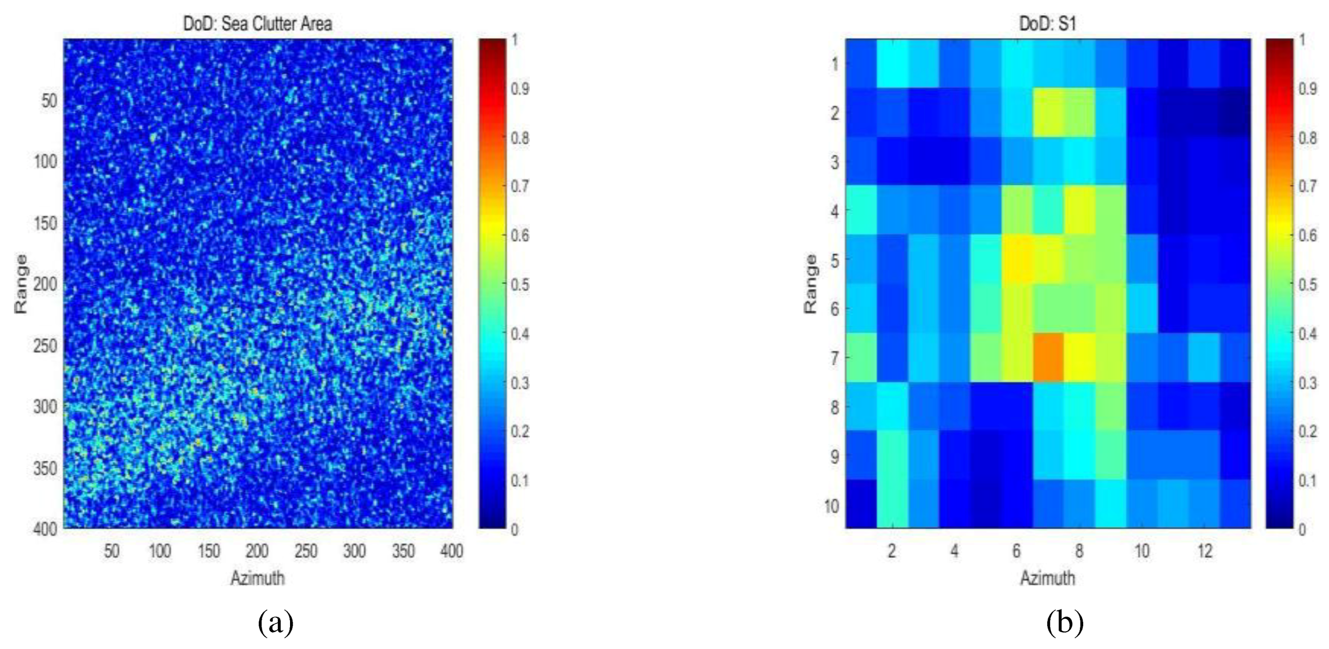
where E is the complex electric field received in the subscripted polarization, and $R(·)$ and $I(·)$ denote the real and imaginary parts of the complex field. Touzi et al. [50] made use of the quad-polarimetric data to demonstrate that an optimization over the all possible DPs was useful for ship detection. Similarly, Shirvany et al. have also demonstrated the effectiveness of the degree of depolarization defined as DoD = 1-DP for ship detection by using dual-pol SAR data [49]. Meanwhile, considering DoD is independent of the transmit polarization and adaptable for on-board implementation [49], we thus choose it as the last extended polarimetric feature vector.

In conclusion, different features have their own advantages and disadvantages. In order to solve the disadvantages of different methods and improve the performance of GP-PNF, new features are added into the feature vector of GP-PNF.

3.2. Constructions of Scattering Vectors

We form the following polarimetric scattering vectors (SV${}_{\mathrm{N}}$), as listed in

Table 1. Scattering vectors.

Name	Vector Description	Dimension
SV${}_1(\mathrm{Original})$	[$\langle |S_{VV}{|}^2\rangle$,$\langle |S_{VH}{|}^2\rangle$,$\langle S_{VV}^{\ast }{S}_{VH}\rangle$]	3
SV${}_{1\mathrm{PCA}}$(Improved)	The first three columns of PCA feature matrix using SV${}_1$	3
SV${}_2$(Improved)	[$\langle |S_{VV}{|}^2\rangle$,$\langle |S_{VH}{|}^2\rangle$,$\langle S_{VV}^{\ast }{S}_{VH}\rangle$,	6
	$\langle SPAN\rangle$,$\langle MTC\rangle$,$\langle DoD\rangle$]
SV${}_{2\mathrm{PCA}}$(Improved)	The first three columns of PCA feature matrix using SV${}_2$	3

:

• SV${}_1$: It is the original feature vector of GP-PNF. We consider these features as they are the basic representations of the PolSAR data directly selected from the covariance matrix [C].
• SV${}_2$: In this paper, we extend the 3D SV${}_1$ vector using three extra polarimetric features, i.e., SPAN, MTC and DoD. They have all been successfully used for ship detection and can effectively supplement the ship polarimetric information in the framework of GP-PNF.
• SV${}_{1\mathrm{PCA}}$ and SV${}_{2\mathrm{PCA}}$: They are feature vectors derived by the first three axes of the basis resulting of PCA. SV${}_{1\mathrm{PCA}}$ has the same dimension as the original SV${}_1$, but the basis used to represent it is different and it is shifted at the center of the data cluster. SV${}_{2\mathrm{PCA}}$ considers a reduction of dimension from 6 to 3 compared to the 6D SV${}_2$ vector.

3.3. The Proposed Ship Detection Method

As shown in Figure 1, the first step is to build a larger feature vector ${\underline{t}}^{{}^{\prime }}$ that contains more polarimetric features:

$${\underline{t}}^{{}^{\prime }}=[\langle |S_{VV}{|}^2\rangle ,\langle |S_{VH}{|}^2\rangle ,\langle |S_{VV}^{\ast }{S}_{VH}|\rangle ,\langle SPAN\rangle ,\langle MTC\rangle ,\langle DoD\rangle ].$$

(13)

Then, the PCA is used to change the basis and reduce the dimensions of ${\underline{t}}^{{}^{\prime }}$. Here, we retain only the first three axes of the final PCA basis and call the resulting vector ${\underline{t}}_{new}$:

$${\underline{t}}_{new}=[|f_1^{PCA}{|}^2,|f_2^{PCA}{|}^2,|f_3^{PCA}{{|}^2]}^T,$$

(14)

where $f_1^{PCA}$ (i = 1, 2, 3) are the new features after the PCA operator.

Since we are evaluating the covariance matrix of a feature vector that contains second order statistics of the target, we are effectively exploiting higher order statistics. Further work will be carried out in the future to understand the importance of considering higher order statistics for this application.

Finally, the final expression of the detector is built as:

$$\begin{array}{cc}\hfill {\gamma }_d& =\frac{1}{\sqrt{1+RedR(\frac{P_{tot}}{P_T}-1)}}\hfill \\ & =\frac{1}{\sqrt{1+RedR(\frac{{\underline{t}}_{new}^{\ast T}{\underline{t}}_{new}}{|{\underline{t}}_{new}^{\ast T}{\underline{\widehat{t}}}_T|}-1)}}\ge T,\hfill \end{array}$$

(15)

where $P_{tot}$ is the power of $t_{new}$, ${\underline{\widehat{t}}}_T$ is a normalized version of the partial target vector ${\underline{t}}_T$ [41] and “T” is a threshold. Here, we also give the pseudocode of the proposed method as shown in Algorithm 1.

Algorithm 1 The proposed ship detection algorithm.

Input: The original SAR data D, $RedR$, k, M, F, $S{V}_{PCA}$, ${\underline{t}}_{new}$, T. Output: The final result.  Extracting the set of reliable negative and/or positive samples $T_n$ from $U_n$ with help of $P_n$;  Converting D into covariance matrices for individual pixel;  Set $RedR$;  For $k=1$ to M;   Get the six scattering features of the pixel based on D;   Put these features into a vector F;   Use PCA to transform F, and obtain a new vector $S{V}_{PCA}$;   Choose the first three columns of $S{V}_{PCA}$ to form the final vector ${\underline{t}}_{new}$;   Adopt Equation (15) to calculate ${\gamma }_d$;  End For;  Set a threshold T to output the final result.

4. Results and Discussion

To demonstrate the effectiveness of the proposed method in PolSAR ship detection, we conduct experiments on four freely available Sentinel-1 datasets. Three conventional detection algorithms, namely, the VH (i.e., HV) detector [46], the MTC detector [47], the degree of depolarization (DoD) detector [49], and the reflection symmetry (RF) detector [18] are used for comparison. On the other hand, a series of Geometrical Perturbation-Polarimetric Notch Filter (GP-PNF) methods (we call “PNF${}_{\mathrm{X}}$” here) [37,38,39] are also adopted for comparison. Thus, a total of eight algorithms are used:

• VH : Amplitude of VH,
• MTC : Product of amplitudes VV and VH,
• DoD : Degree of depolarization,
• RS : Reflection symmetry,
• PNF${}_{3\mathrm{D}}$ : Using the SV${}_1$ feature vector (Original),
• PNF${}_{6\mathrm{D}}$ : Using the SV${}_2$ feature vector (Proposed),
• PNF${}_{3\mathrm{DPCA}}$ : Using the SV${}_{1\mathrm{PCA}}$ feature vector (Proposed),
• PNF${}_{6\mathrm{DPCA}}$ : Using the SV${}_{2\mathrm{PCA}}$ feature vector (Proposed).

All experiments are mainly carried out on a computer with an i7-6770HQ CPU of 2.60 GHz and a memory of 12 GB.

4.1. Datasets

In this paper, four Sentinel-1 IW dual-pol scenes are adopted to evaluate the proposed method. The first scene was acquired in the harbor of Panama City on 25 November 2015, which had a clam sea state. Its VH amplitude image and optical image obtained from Google Earth are shown in Figure 2. In order to avoid the influence of land, one subarea called ‘A’ is further selected from the harbor as our experimental dataset (see Figure 2c). This is highlighted by the green box (550 × 990 in pixels) in Figure 2b. The red area (400 × 400) is randomly chosen as the sample area of sea clutter in Figure 2b. The second scene was acquired in the harbor of Gibraltar on 13 June 2016. The optical and VH amplitude images are shown in Figure 2d,e. Similarly, we choose one subarea called ‘B’ as our experimental dataset (see Figure 2f), which is also highlighted by the green box (740 × 950) in Figure 2e. The sample area of sea clutter is still randomly chosen and indicated by a red box (400 × 400) in Figure 2e. Note that the sea state of B is rougher than that of A. The third scene was acquired in the English Channel on 12 January 2017, whose corresponding optical image is shown in Figure 2g. The VH amplitude image of dataset ‘C’ (3597 × 5273 in pixels) is shown in Figure 2h. Compared to A and B, C has the roughest sea state. The last dataset ‘D’ (1101 × 781 in pixels) was obtained in East China Sea on 12 December 2016, where the ocean state is as rough as that of C. Its related optical and VH amplitude image are shown in Figure 2i,j. It should be mentioned that the oceanographic data, i.e., Wind Level, was collected from the UK Met Office [51] and the National Meteorological Center of CMA [52].

Table 2. Parameters of the Sentinel-1 Datasets.

Scene	Product	Polarization	Range Pixel	Azimuth Pixel	PRF	Azimuth	Range	Wind	Time	Data
	Type		Space (m)	Space (m)	(Hz)	Looks	Looks	Level		Site
A	SLC	VV/VH	2.3296	14.0117	1717.129	1	1	1–3	25 November 2015 23:31:23	Panama City
B	SLC	VV/VH	2.3296	13.9372	1717.129	1	1	3–5	13 June 2016 18:17:46	Gibraltar
C	SLC	VV/VH	2.3296	13.8990	1717.129	1	1	6–9	12 January 2017 17:56:51	English Channel
D	SLC	VV/VH	2.3296	13.9556	1717.129	1	1	6–7	12 December 2016 09:45:56	East China Sea

lists all the acquisition parameters of the four datasets.

To evaluate ship detection performance, the ground truth data should be given, in which the ship locations are marked. However, we do not have the ground truth data corresponding to the four datasets, especially the AIS information. Instead, we mainly determine the locations of ships by visual inspection in this paper.

4.2. Evaluation Criteria

In order to evaluate the detection performance of the different methods, we need some validating datasets with the positions of ships in the images. In this work, we determined the locations of real ships by visual inspection of the SAR images. The detection results are all expressed in binary format, where white represents ships and black represents sea clutter. The threshold for each detector was selected manually in order to obtain the best detection mask with the highest possible probability of detection $P_d$ and the lowest possible probability of false alarm $P_f$. This is to emulate a perfect statistical methodology that is able to find the best threshold possible.

The previous methodology still requires the selection of a threshold that may not be fully optimal. In order to avoid any possible mistake in selecting the threshold, we perform some quantitative analyses that are independent from the selection of the thresholds. We adopt the Receive Operating Characteristic (ROC) curve, which is a plot showing probability of detection against probability of false alarms while the threshold is varied. The probabilities are defined as:

$$\left\{\begin{array}{cc}\hfill P_d& =\frac{N_{dt}}{N_{tp}},\hfill \\ \hfill P_f& =\frac{N_{fp}}{N_{cp}},\hfill \end{array}\right.$$

(16)

where $N_{dt}$ is the number of detected target pixels, $N_{tp}$ denotes the number of all target pixels, $N_{fp}$ indicates the number of false alarm pixels, and $N_{cp}$ represents the number of sea clutter pixels.

Additionally, we use the Target-to-Clutter Ratio (TCR) as another indicator of detection performance. The higher TCR is, the better separation we have between targets and clutter, and therefore the better the detection performance is. TCR is evaluated in dB as:

$$TCR=10{\log }_{10}\left(\frac{I_T}{I_C}\right)$$

(17)

where $I_T$ and $I_C$ denote the values of the square of target power $P_T$ for target and clutter, respectively. $I_T$ is calculated by identifying the geometrical center of ships in the image and averaging the surrounding values of $P_T$ for bright pixels. For $I_C$, we randomly select one sea area (400 × 400) as the sample area of sea clutter and averaged the $P_T$ of 160,000 pixels. This is because the square of $P_T$ has the same dimension of the intensity of VH and therefore provides a fair comparison between the detectors.

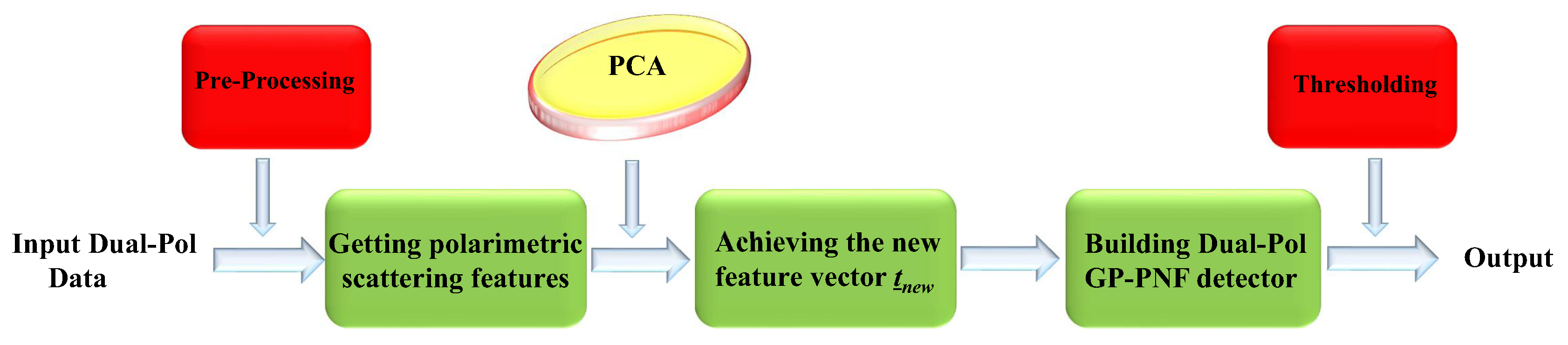
4.3. Results and Discussions on the First Sentinel-1 Dataset

Figure 2c shows the VH image of the dataset A, which includes 25 real ships. Here, we use the orange circles for highlighting them. Please note, to have a fair comparison in all PNF${}_{\mathrm{X}}$ algorithms, we keep the parameters of window size the same: WinTrain = 75, WinTest = 7. In addition, the size of averaging window used for other detectors is 3 × 3 except for the VH and RS detectors. These parameters are selected to produce the best performance for the specific algorithm.

As a matter of fact, the sea surface of A is the calmest among these four datasets. Since the main concern of the proposed method is detection with rough sea state, we briefly report the detected results of A as a comparison for better understanding the improvements in rough conditions.

Overall, we can find that the results of VH${}_{\mathrm{filter}}$, MTC and all the PNF${}_{\mathrm{X}}$ methods seem to all be very good. VH${}_{\mathrm{filter}}$ and MTC are shown in Figure 3b,c. They detect all the 25 ships with no false alarms. This implies that, after filtering, the amplitude information of VH channel may be enough for distinguishing ships from sea clutter when the sea state is calm. Comparing with Figure 3b, the result of the VH detector shown in Figure 3a also demonstrates the effectiveness of filtering. Figure 3d shows the result of DoD that detects no ships and some false alarms. The result of RS is shown in Figure 3e. Obviously, not all of the ship pixels are detected, though the structures of detected ships are visible. From Figure 3f–i, we can see that the results of a series of PNF${}_{\mathrm{X}}$ detectors, namely, PNF${}_{3\mathrm{D}}$, PNF${}_{3\mathrm{DPCA}}$, PNF${}_{6\mathrm{D}}$ and PNF${}_{6\mathrm{DPCA}}$, are similar. They detect all ships with no false alarms. This means that just using the original model of PNF (SV${}_1$) in the case of calm sea state is sufficient for detecting ships, thus the PCA operator is not necessary.

To sum up, when the sea state is calm, many traditional methods are able to detect ships effectively, and the proposed algorithms may not have a significant advantage.

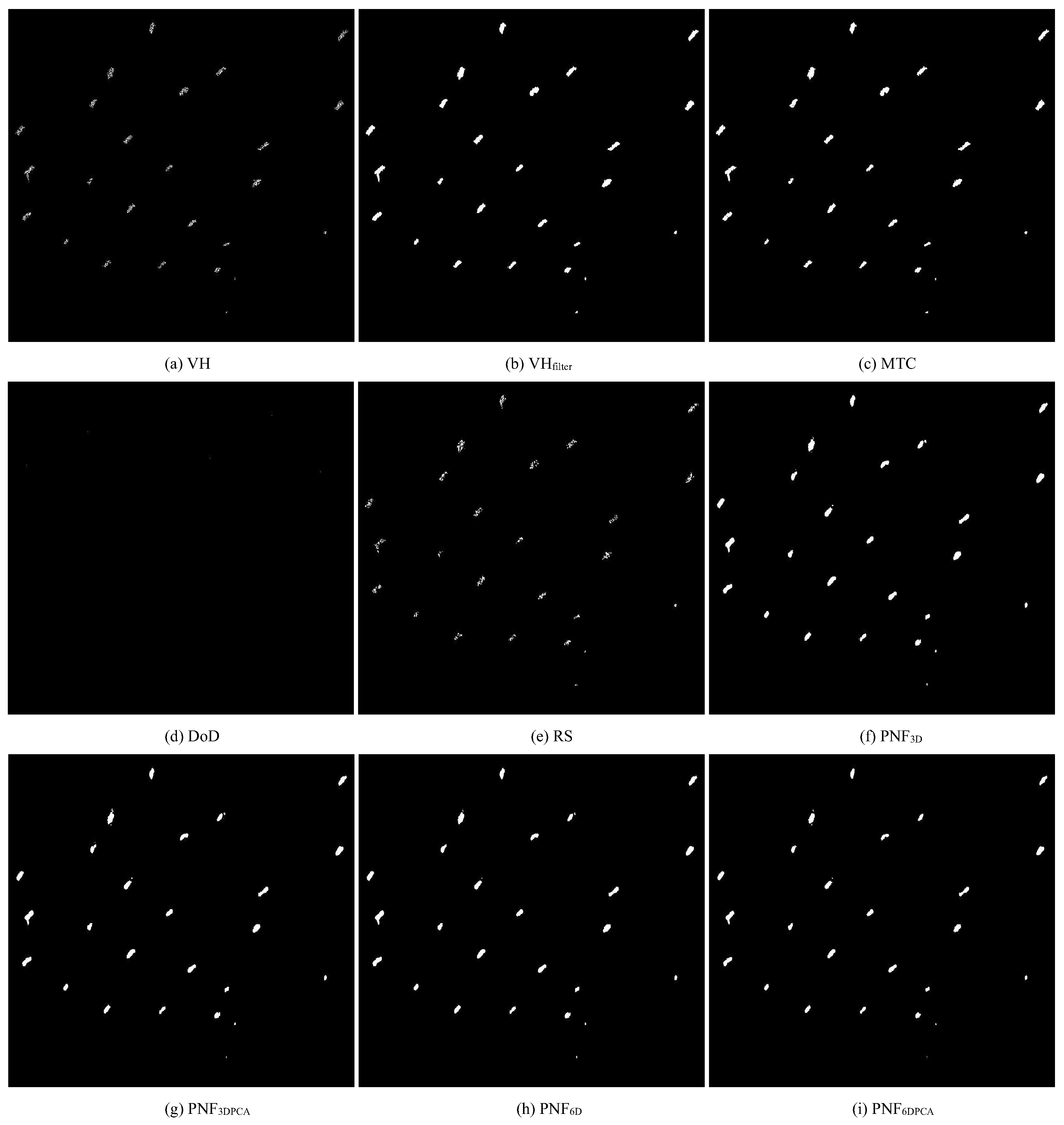
4.4. Results and Discussions on the Second Sentinel-1 Dataset

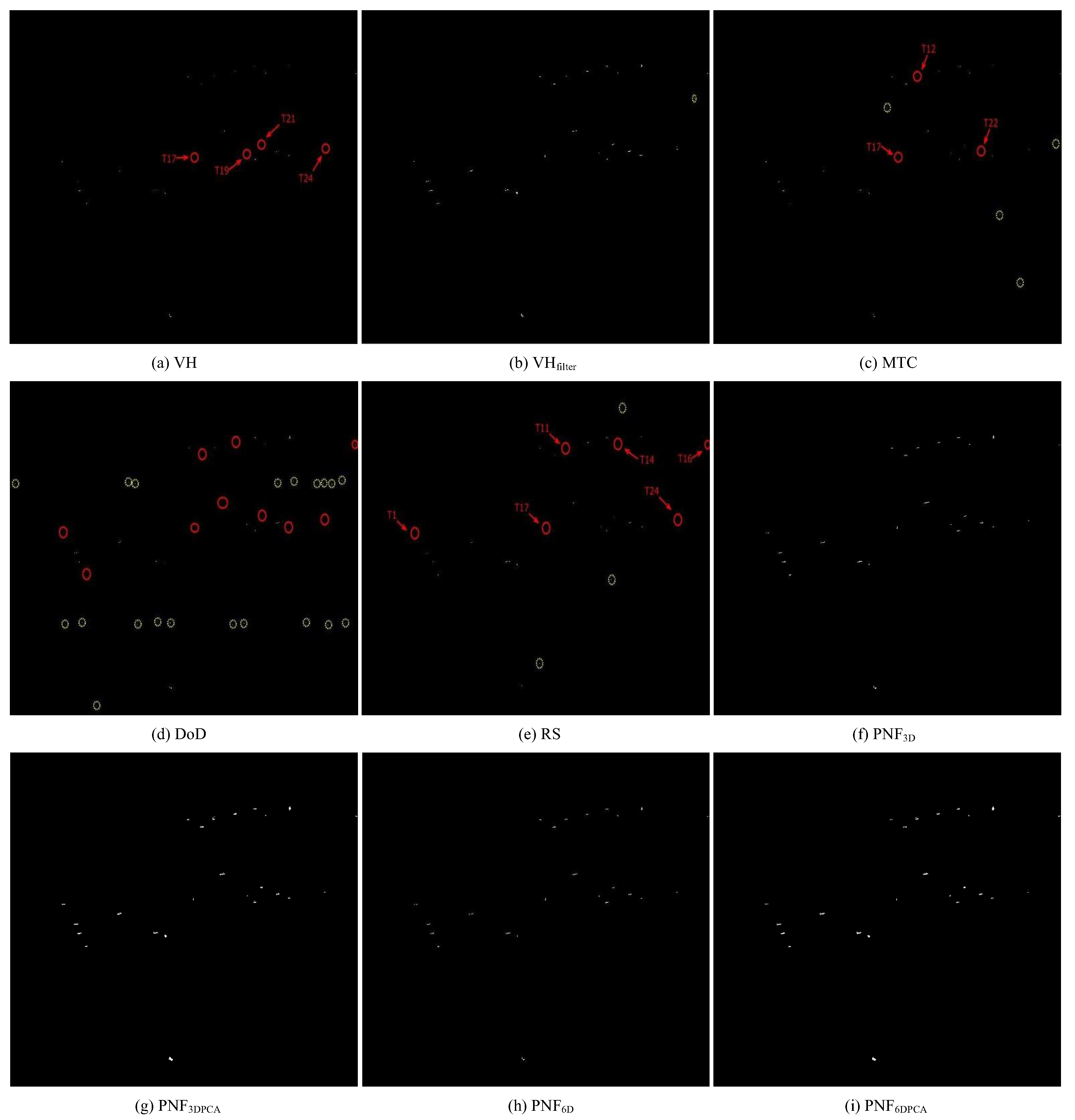
The VH image of the dataset B is shown in Figure 2e, which consists of 19 visually identified ships. To make it clearer, we also mark all the real ships with orange circles and use orange dashed circles to represent three ships S1, S2 and S3, which present much weaker backscattering. The averaging window sizes used for other detectors are showed in the top of

Table 3. TCR values of smaller ships and average TCR values of 19 ships of B (dB).

	Methods	VH	VH${}_{\mathbf{filter}}$	MTC	DoD	RS	PNF${}_{3\mathbf{D}}$	PNF${}_{3\mathbf{DPCA}}$	PNF${}_{6\mathbf{D}}$	PNF${}_{6\mathbf{DPCA}}$	$\Delta$TCR
Ships		(None)	(3 × 3)	(3 × 3)	(3 × 3)	(7 × 7)
S1 (L:33 m, W:14 m)		$5.37$	$4.73$	$7.67$	$3.33$	$4.38$	$8.37$	$8.54$	$8.79$	$\mathbf{9.0}$	$0.63$
S2 (L:72 m, W:24 m)		$4.81$	$4.29$	$6.68$	$3.38$	$5.17$	$6.77$	$6.98$	$7.17$	$\mathbf{7.38}$	$0.61$
S3 (L:65 m, W:10 m)		$7.31$	$5.97$	$9.18$	$4.70$	$4.41$	$8.99$	$9.16$	$9.43$	$\mathbf{9.65}$	$0.66$
S4 (L:125 m, W:20 m)		$6.82$	$6.76$	$9.30$	$5.56$	$5.80$	$13.83$	$13.88$	$14.23$	$\mathbf{14.38}$	$0.55$
$\mathit{Average}\mathit{Values}$		$6.71$	$6.41$	$8.99$	$4.88$	$6.77$	$12.10$	$12.21$	$12.29$	$\mathbf{12.47}$	$0.37$

(·): The size of the averaging window; $\Delta$TCR: The difference of TCR values between PNF${}_{\mathbf{6}\mathbf{DPCA}}$ and PNF${}_{\mathbf{3}\mathbf{D}}$; L(m): The length of ship; W(m): The width of ship.

.

Figure 4 gives the results of all the detectors. The red circles identify the missed ships and yellow dashed circles mean false alarms. The detection mask of DoD shows very few detected ships. This is because the sea clutter is strong and ships often have a low DoD value. To keep the $P_f$ low, we had to set a threshold very high; thus, in this dataset, almost nothing could be detected using DoD, as shown in Figure 4d. Taking S1 as example, Figure 5 shows that its DoD values are not much higher than the ones of sea clutter. Using an optimization of DP with quad-polarimetric data may improve the final detection mask.

As discussed earlier, many ships have a stronger backscattering in the VH channel compared to the sea surface. Again, the result of Figure 4b demonstrates that the cross-polarized channel after filtering can make the outlines of ships much clearer compared to Figure 4a and be useful for detecting the weaker ships. The results of MTC shown in Figure 4c presents a similar performance to VH.

Figure 4e shows the result of RS. Though many bigger ships are detected effectively, all of the weaker ships are still missing due to their low RS values. As shown in Figure 6, we can observe that the difference of RS values between S1 and its surrounding sea clutter pixels is small.

With respect to a series of PNF${}_{\mathrm{X}}$ methods, Figure 4f–i depict their results. To have a fair comparison in all PNF${}_{\mathrm{X}}$ algorithms, we also keep their parameters of window size the same here: WinTrain = 75, WinTest = 7. By visual comparison, it is evident that all the PNF${}_{\mathrm{X}}$ methods have good results because all of the weaker ships are detected.

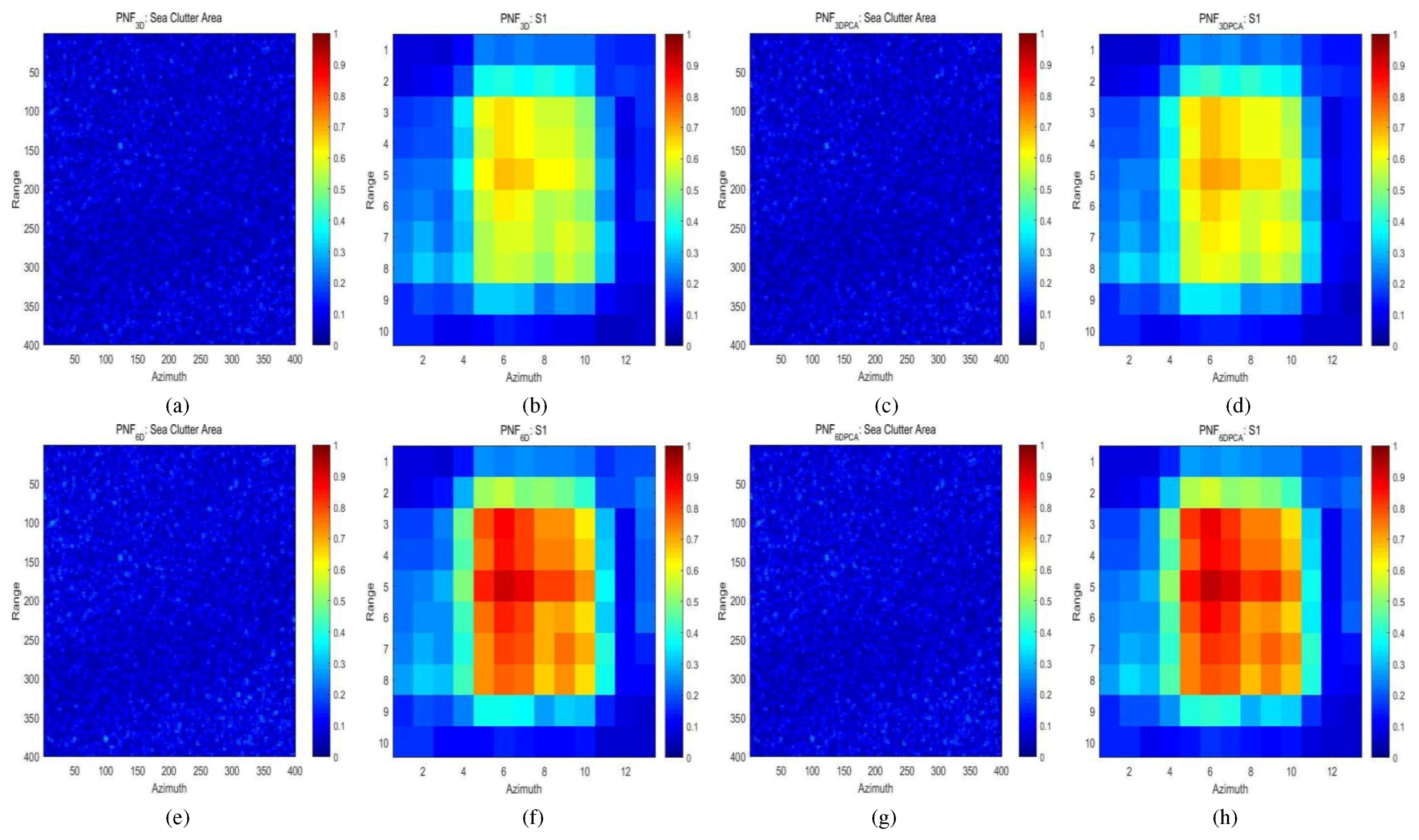
Here, we still choose S1 as an example. Figure 7 shows the $P_T$ values of the PNF${}_{\mathrm{X}}$ algorithms, which is the key metric of the PNF${}_{\mathrm{X}}$ detectors. The $P_T$ values of S1 for the 6D vector are higher compared to the 3D vector. This is because adding features can help us increase the total power of the 6D vector, which also increases a bit of the $P_T$ for the clutter area.

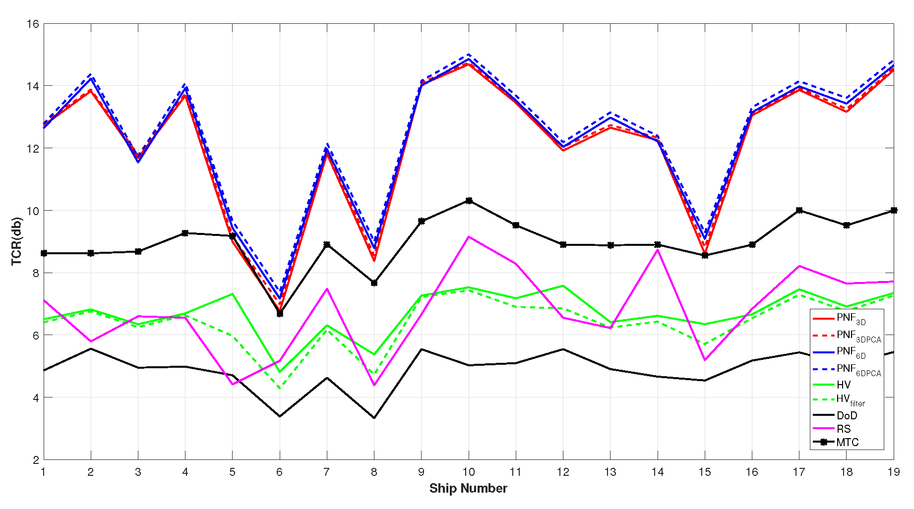
To better understand if there is a gain in the detection performance, here, we list the TCR values of S1, S2, S3 and S4 (a larger ship) in Table 3. As shown in Table 3, the TCR values of PNF${}_{6\mathrm{DPCA}}$ are the highest. This means that the ship pixels can be more easily detected by setting an appropriate threshold. Comparing PNF${}_{3\mathrm{D}}$ and PNF${}_{3\mathrm{DPCA}}$ or PNF${}_{6\mathrm{D}}$ and PNF${}_{6\mathrm{DPCA}}$, we can find that TCR is further enhanced by using PCA. For example, TCR of S1 is enhanced about 0.11 dB for PNF${}_{3\mathrm{D}}$ and 0.18 dB for PNF${}_{6\mathrm{D}}$. PCA sets the basis of the feature vector so that it aligns with the axis where the sea clutter is mostly present or less present. In addition, it moves the center of the axis in the middle of the distribution, allowing a better angle separation between target and clutter dimensions. As shown in Figure 8, we can observe that the TCR value of each ship is enhanced by PNF${}_{6\mathrm{DPCA}}$. Moreover, the average TCR value of these 19 ships is also listed in the bottom of Table 3 (italics). Compared to PNF${}_{3\mathrm{D}}$, the average TCR enhancement of PNF${}_{6\mathrm{DPCA}}$ is 0.37 dB. However, the enhancement for some weak ships like S1 is larger, i.e., 0.63 dB.

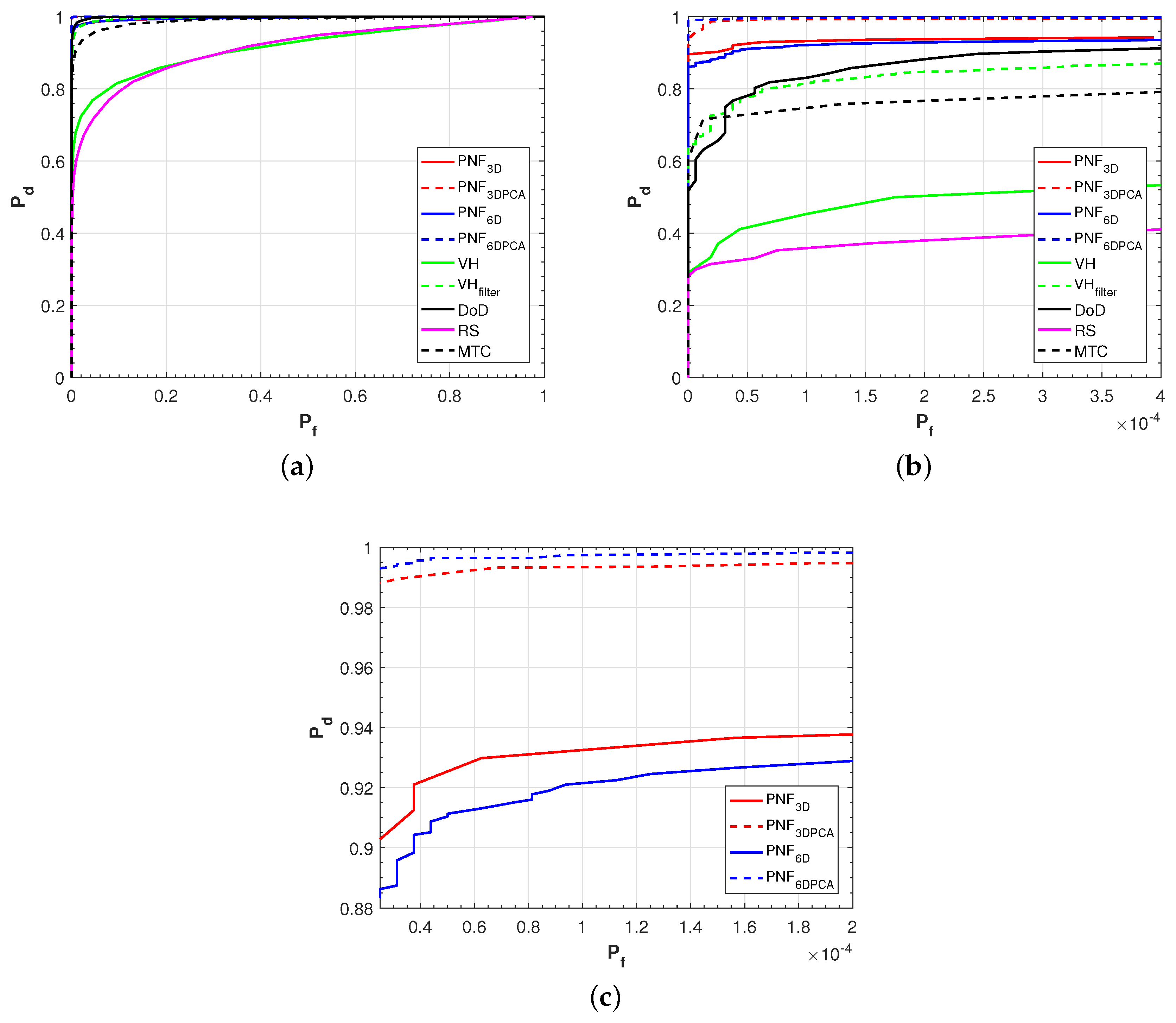
Here, to have a better look at the PNF${}_{\mathrm{X}}$ detectors, we zoom in on their ROC curves in Figure 9c. We can find that PNF${}_{6\mathrm{DPCA}}$ has the best performance. In these ranges of $P_f$ values, $P_d$ is on average higher of 0.014 compared to PNF${}_{3\mathrm{D}}$.

Figure 9 presents the ROC curves of these detectors, which can allow a fair comparison independently of the specific thresholds. As shown in Figure 9a, we can find that the PNF${}_{\mathrm{X}}$ detectors have the best performance among these nine detectors. Zooming in on the ROC curves with $P_f$ smaller than 10${}^{-4}$, the curve of MTC is close to the curve of VH${}_{\mathrm{filter}}$.

4.5. Results and Discussions on the Third Sentinel-1 Dataset

Figure 2h depicts the third dataset C with 24 ships, whose size is 3597 × 5273 in pixels and has a wider sea area. According to the weather reported [52], we know that it has a stronger wind level (6–9 in Beaufort scale) compared to A and B. We select this dataset to verify the effectiveness of the proposed method when the sea condition is very harsh.

Compared to Figure 4a, we can also find that ships of C appear less bright in the VH channel, and this is because the sea clutter is stronger. Figure 10a shows the result of the VH detector, where we can find that some ships are missing. VH${}_{\mathrm{filter}}$ is able to detect smaller ships but still detect one false alarm (Figure 10b). The result of MTC is also shown in Figure 10c, which has some missing ships and false alarms. It seems that DoD (Figure 10d) can detect few ships, but also detect many false alarms. Similarly, Figure 10e presents the result of RS, which misses some ships and has few false alarms.

Figure 10f–i present the results of the PNF${}_{\mathrm{X}}$ methods where we cannot see false alarms. It can be observed that all four of the methods achieve good results where they detect all the 24 real ships effectively. However, the detected ships of PNF${}_{3\mathrm{DPCA}}$ and PNF${}_{6\mathrm{DPCA}}$ are much clearer. Note that, in order to have a fair comparison in all PNF${}_{\mathrm{X}}$ algorithms, we still make them have the same parameters here: WinTrain = 75, WinTest = 7.

Taking the ship T5 as an example, Figure 11 gives the $P_T$ values of T5. We can find that PNF${}_{6\mathrm{DPCA}}$ has the largest values. In addition, the pixels of T5 are the brightest and most complete. All the TCR values of these 24 ships are also listed in

Table 4. TCR values of smaller ships and average TCR values of 24 ships of B (dB).

	Methods	VH	VH${}_{\mathbf{filter}}$	MTC	DoD	RS	PNF${}_{3\mathbf{D}}$	PNF${}_{3\mathbf{DPCA}}$	PNF${}_{6\mathbf{D}}$	PNF${}_{6\mathbf{DPCA}}$	$\Delta$TCR
Ships		(none)	(3 × 3)	(3 × 3)	(3 × 3)	(7 × 7)
T1 (L:166 m, W:54 m)		$5.91$	$5.58$	$6.77$	$6.56$	$3.80$	$9.25$	$11.37$	$9.56$	$\mathbf{11.30}$	$2.05$
T2 (L:198 m, W:70 m)		$6.19$	$6.06$	$7.40$	$7.10$	$4.47$	$10.79$	$12.99$	$10.91$	$\mathbf{13.19}$	$2.40$
T3 (L:174 m, W:63 m)		$6.84$	$6.70$	$8.03$	$7.31$	$5.03$	$11.63$	$13.78$	$11.70$	$\mathbf{13.88}$	$2.25$
T4 (L:120 m, W:41 m)		$5.82$	$5.74$	$7.04$	$6.61$	$5.15$	$10.14$	$12.28$	$10.28$	$\mathbf{12.56}$	$2.42$
T5 (L:160 m, W:50 m)		$5.32$	$5.23$	$5.64$	$6.73$	$5.20$	$8.48$	$12.51$	$8.20$	$\mathbf{12.68}$	$4.2$
T6 (L:224 m, W:73 m)		$6.13$	$6.00$	$7.09$	$7.01$	$4.81$	$10.71$	$12.87$	$10.76$	$\mathbf{13.05}$	$2.34$
T7 (L:204 m, W:58 m)		$6.79$	$6.58$	$8.20$	$7.05$	$5.83$	$11.16$	$13.37$	$11.25$	$\mathbf{13.70}$	$2.54$
T8 (L:64 m, W:27 m)		$6.57$	$6.51$	$7.78$	$6.96$	$6.92$	$11.16$	$14.11$	$10.98$	$\mathbf{14.42}$	$3.26$
T9 (L:108 m, W:40 m)		$4.95$	$4.87$	$5.79$	$6.13$	$5.12$	$8.87$	$10.54$	$8.98$	$\mathbf{10.94}$	$2.07$
T10 (L:168 m, W:56 m)		$6.73$	$6.53$	$8.03$	$7.07$	$6.17$	$11.27$	$13.23$	$11.36$	$\mathbf{13.45}$	$2.18$
T11 (L:130 m, W:46 m)		$6.22$	$6.01$	$7.44$	$6.94$	$4.22$	$9.94$	$12.33$	$10.09$	$\mathbf{12.44}$	$2.50$
T12 (L:150 m, W:51 m)		$5.67$	$5.61$	$6.58$	$6.83$	$4.35$	$9.88$	$12.17$	$9.97$	$\mathbf{12.28}$	$2.40$
T13 (L:147 m, W:49 m)		$5.92$	$5.85$	$7.11$	$6.54$	$6.47$	$10.48$	$12.49$	$10.51$	$\mathbf{12.73}$	$2.25$
T14 (L:48 m, W:23 m)		$6.24$	$6.01$	$7.52$	$6.68$	$5.22$	$10.27$	$12.42$	$10.38$	$\mathbf{12.69}$	$2.42$
T15 (L:285 m, W:48 m)		$5.61$	$5.60$	$7.15$	$6.67$	$5.90$	$10.27$	$11.83$	$10.52$	$\mathbf{12.32}$	$2.05$
T16 (L:96 m, W:27 m)		$6.05$	$6.02$	$7.17$	$6.98$	$4.98$	$9.77$	$13.35$	$9.55$	$\mathbf{13.78}$	$4.01$
T17 (L:138 m, W:30 m)		$5.77$	$5.57$	$6.78$	$6.75$	$4.04$	$9.32$	$11.08$	$9.54$	$\mathbf{11.26}$	$1.94$
T18 (L:278 m, W:84 m)		$5.84$	$5.73$	$7.16$	$6.50$	$4.66$	$9.52$	$12.15$	$9.61$	$\mathbf{12.50}$	$2.98$
T19 (L:54 m, W:24 m)		$6.14$	$5.96$	$7.48$	$6.81$	$3.39$	$10.45$	$12.35$	$10.83$	$\mathbf{12.48}$	$2.03$
T20 (L:181 m, W:53 m)		$6.72$	$6.46$	$7.79$	$7.04$	$5.25$	$10.64$	$12.96$	$10.71$	$\mathbf{13.03}$	$2.39$
T21 (L:126 m, W:33 m)		$6.12$	$6.05$	$7.23$	$6.86$	$6.15$	$10.46$	$12.98$	$10.55$	$\mathbf{12.95}$	$2.49$
T22 (L:173 m, W:52 m)		$6.55$	$6.29$	$7.29$	$7.12$	$6.30$	$10.94$	$13.11$	$10.90$	$\mathbf{13.31}$	$2.37$
T23 (L:133 m, W:31 m)		$5.88$	$5.68$	$6.93$	$6.54$	$6.51$	$9.91$	$11.70$	$10.04$	$\mathbf{12.23}$	$2.32$
T24 (L:64 m, W:15 m)		$5.92$	$5.64$	$6.81$	$6.82$	$2.52$	$9.34$	$11.31$	$9.58$	$\mathbf{11.39}$	$2.05$
$\mathit{Average}\mathit{Values}$		$6.08$	$5.93$	$7.18$	$6.82$	$5.10$	$10.20$	$12.47$	$10.29$	$\mathbf{12.70}$	$2.50$

(·): The size of the averaging window; $\Delta$TCR: The difference of TCR values between PNF${}_{\mathbf{6}\mathbf{DPCA}}$ and PNF${}_{\mathbf{3}\mathbf{D}}$; L(m): The length of ship; W(m): The width of ship.

. The enhancement of the TCR is largest for the PNF${}_{6\mathrm{DPCA}}$ detector. Compared with PNF${}_{3\mathrm{D}}$, the difference in TCR, $\Delta$TCR is 2.50 dB, which is higher than that of B (0.37 dB). This shows how PNF${}_{6\mathrm{DPCA}}$ is most effective in improving the TCR values of ships when the sea condition is very high.

Interestingly, we notice that PNF${}_{6\mathrm{D}}$ only enhances the average TCR about 0.09 dB compared to PNF${}_{3\mathrm{D}}$. This is lower than that of dataset B (0.19 dB). It can be deduced that the improvement in rough sea condition comes mostly from the PCA methodology more than the inclusion of more features in the vector. Comparing B and C, $\Delta$TCR values of PNF${}_{3\mathrm{DPCA}}$ are 0.11 dB and 2.27 dB, respectively. The $\Delta$TCR values of PNF${}_{6\mathrm{DPCA}}$ are 0.37 dB and 2.5 dB, respectively.

We also present the ROC curves of these detectors in Figure 12. We can see that all the PNF${}_{\mathrm{X}}$ detectors have better performance than the other algorithms. Zooming in on the ROC curves with $P_f$ smaller than 5 × 10${}^{-4}$, the performance of the VH${}_{\mathrm{filter}}$ detector is best among all the traditional algorithms when $P_f$ is smaller than 10${}^{-5}$ (Figure 12b). When the sea condition is rough, the curves of PNF${}_{3\mathrm{DPCA}}$ and PNF${}_{6\mathrm{DPCA}}$ show a much clearer improvement compared to PNF${}_{3\mathrm{D}}$ and PNF${}_{6\mathrm{D}}$ (Figure 12c). The $P_d$ value of PNF${}_{6\mathrm{DPCA}}$ approaches to 0.995 when $P_f$ is around 10${}^{-5}$. We can observe that the curve of PNF${}_{6\mathrm{D}}$ is lower than that of PNF${}_{3\mathrm{D}}$. This is another confirmation that the biggest benefit in rough sea conditions comes from the PCA method and not the adding of extra features that may be strongly correlated to each other.

4.6. Results and Discussions on the Fourth Sentinel-1 Dataset

The fourth dataset D (1101 × 781 in pixels), shown in Figure 2j, is composed of 37 real ships. Except for the fact that a high wind (6–7 in Beaufort scale) [52] is present in this scene, the dataset D also includes more smaller ships, which may be small fishing vessels because of the developed fishery in the East China Sea. Therefore, it is chosen as a challenging scene here. By visual inspection in Figure 2j, we can further find that these smaller ships are mostly submerged in the background clutter.

For the sake of saving space, here, we just show the results of different methods. Figure 13a shows the result of VH, which misses nine smaller ships and detects some false alarms simultaneously. Compared to VH, VH${}_{\mathrm{filter}}$ (Figure 13b) detects more smaller ships, though one false alarm is also detected. Again, this proves that filtering is helpful for ship detection in the case of a high ocean state. Figure 13c depicts the result of MTC. We can find that more smaller ships are missed and two false alarms are also detected. The result of DoD seems to be worst, as shown in Figure 13d. It includes many missing ships and false alarms. The result of RS represented in Figure 13e also reflects that RS may be not very useful for detecting smaller ships when the background clutter is strong.

Based on the same parameters (WinTrain = 75, WinTest = 7), here, we also show the results of the PNF${}_{\mathrm{X}}$ methods in Figure 13f–i. Observing Figure 13f, we can find that PNF${}_{3\mathrm{D}}$ detect the most of ships, but still misses two smaller ships and detects two false alarms. Compared to Figure 13f, we can see that PNF${}_{3\mathrm{DPCA}}$ (Figure 13g) exhibits a better performance of detecting ships than PNF${}_{3\mathrm{D}}$ because no smaller ships and false alarms are detected. This further demonstrates the effectiveness of adopting PCA. Figure 13h depicts the result of PNF${}_{6\mathrm{D}}$. Even if PNF${}_{6\mathrm{D}}$ detects none false alarms, it still misses one smaller ship. Figure 13i gives the result of PNF${}_{6\mathrm{DPCA}}$. All 37 of the targets are correctly detected with no false alarms.

In this challenging scene, PNF${}_{6\mathrm{DPCA}}$ shows more clearly the ability to improve detection performances, especially for smaller ships.

5. Conclusions

By using the framework of GP-PNF and PCA, we explore two types of ship detection algorithms. One considers just extending the number of features in the polarimetric feature vector used by GP-PNF. Another considers a PCA method on the feature vector before applying GP-PNF. The new algorithms are tested on four real Sentinel-1 datasets. The results verify the effectiveness of the proposed methods, especially in the case of a rough sea state. The key contributions of this work are listed as follows:

• Adding more polarimetric features, which can more effectively reflect the difference between ships and clutter, in the original feature vector of the dual-pol GP-PNF method. Thus, the feature vector is extended from three to six dimensions.
• Based on the 6D vector, we use the PCA method to reduce again the space to three dimensions. The experiments tested on four real Sentinel-1 datasets confirm that the PCA operation is useful. In particular, the smaller ships can be more effectively detected after PCA when the ocean condition is higher. Meanwhile, we also demonstrate that only adding polarimetric features in the feature vector may be not effective when high sea condition appears.

In addition, we also test the performance against other detectors, showing better performance of the PNF${}_{\mathrm{X}}$ algorithms where the PNF${}_{6\mathrm{DPCA}}$ gives the best performance in the case of a high sea state. As a future work, more datasets from other sensors should be analyzed with special interest for quad-polarimetric data.

References

- Lessing, P.; Bernard, L.; Tetreault, B.; Chaffin, J. Use of the automatic identification system (AIS) on autonomous weather buoys for maritime domain awareness applications. In Proceedings of the OCEANS 2006, Boston, MA, USA, 18–21 September 2006; pp. 1–6. [Google Scholar]
- Velotto, D.; Soccorsi, M.; Lehner, S. Azimuth ambiguities removal for ship detection using full polarimetric X-band SAR data. In Proceedings of the 2012 IEEE International Geoscience and Remote Sensing Symposium (IGARSS), Munich, Germany, 22–27 July 2012; pp. 7621–7624. [Google Scholar]
- Lee, J.S.; Pottier, E. Polarimetric Radar Imaging: From Basics to Applications; CRC Press: Boca Raton, FL, USA, 2009. [Google Scholar]
- Copeland, A.C.; Ravichandran, G.; Trivedi, M.M. Localized Radon transform-based detection of ship wakes in SAR images. IEEE Trans. Geosci. Remote Sens. 1995, 33, 35–45. [Google Scholar] [CrossRef]
- Vachon, P.; Campbell, J.; Bjerkelund, C.; Dobson, F.; Rey, M. Ship detection by the RADARSAT SAR: Validation of detection model predictions. Can. J. Remote Sens. 1997, 23, 48–59. [Google Scholar] [CrossRef]
- Eldhuset, K. An automatic ship and ship wake detection system for spaceborne SAR images in coastal regions. IEEE Trans. Geosci. Remote Sens. 1996, 34, 1010–1019. [Google Scholar] [CrossRef]
- Leng, X.; Ji, K.; Yang, K.; Zou, H. A bilateral CFAR algorithm for ship detection in SAR images. IEEE Geosci. Remote Sens. Lett. 2015, 12, 1536–1540. [Google Scholar] [CrossRef]
- Tello, M.; López-Martínez, C.; Mallorqui, J.J. A novel algorithm for ship detection in SAR imagery based on the wavelet transform. IEEE Geosci. Remote Sens. Lett. 2005, 2, 201–205. [Google Scholar] [CrossRef]
- Chaney, R.; Burl, M.; Novak, L. On the performance of polarimetric target detection algorithms. In Proceedings of the IEEE International Radar Conference, Arlington, VA, USA, 7–10 May 1990; pp. 520–525. [Google Scholar]
- Goodman, N.R. Statistical analysis based on a certain multivariate complex Gaussian distribution (an introduction). Ann. Math. Stat. 1963, 34, 152–177. [Google Scholar] [CrossRef]
- Novak, L.M.; Burl, M.C.; Irving, W.; Owirka, G. Optimal polarimetric processing for enhanced target detection. In Proceedings of the National Telesystems Conference, Atlanta, GA, USA, 26–27 March 1991; pp. 69–75. [Google Scholar]
- Liu, T.; Lampropoulos, G. A new polarimetric CFAR ship detection system. In Proceedings of the Geoscience and Remote Sensing Symposium (IGARSS), Denver, CO, USA, 31 July–4 August 2006; pp. 137–140. [Google Scholar]
- Sugimoto, M.; Ouchi, K.; Nakamura, Y. On the novel use of model-based decomposition in SAR polarimetry for target detection on the sea. Remote Sens. Lett. 2013, 4, 843–852. [Google Scholar] [CrossRef]
- Wang, J.; Huang, W.; Yang, J.; Chen, P.; Zhang, H. Polarization scattering characteristics of some ships using polarimetric SAR images. In Proceedings of the International Society for Optics and Photonics SAR Image Analysis, Modeling, and Techniques XI, Prague, Czech Republic, 19–22 September 2011; Volume 8179, p. 81790W. [Google Scholar]
- Touzi, R.; Charbonneau, F. Characterization of target symmetric scattering using polarimetric SARs. IEEE Trans. Geosci. Remote Sens. 2002, 40, 2507–2516. [Google Scholar] [CrossRef]
- Cameron, W.L.; Youssef, N.N.; Leung, L.K. Simulated polarimetric signatures of primitive geometrical shapes. IEEE Trans. Geosci. Remote Sens. 1996, 34, 793–803. [Google Scholar] [CrossRef]
- Cloude, S.R.; Pottier, E. An entropy based classification scheme for land applications of polarimetric SAR. IEEE Trans. Geosci. Remote Sens. 1997, 35, 68–78. [Google Scholar] [CrossRef]
- Nunziata, F.; Migliaccio, M.; Brown, C.E. Reflection symmetry for polarimetric observation of man-made metallic targets at sea. IEEE J. Ocean. Eng. 2012, 37, 384–394. [Google Scholar] [CrossRef]
- Yang, J.; Peng, Y.N.; Lin, S.M. Similarity between two scattering matrices. Electron. Lett. 2001, 37, 193–194. [Google Scholar] [CrossRef]
- Yang, J.; Zhang, H.; Yamaguchi, Y. GOPCE-based approach to ship detection. IEEE Geosci. Remote Sens. Lett. 2012, 9, 1089–1093. [Google Scholar] [CrossRef]
- Marino, A.; Woodhouse, I.H. Selectable target detector using the polarization fork. In Proceedings of the IEEE Geoscience and Remote Sensing Symposium (IGARSS), Cape Town, South Africa, 12–17 July 2009; Volume 3. [Google Scholar]
- Marino, A.; Cloude, S.R.; Woodhouse, I.H. Detecting depolarized targets using a new geometrical perturbation filter. IEEE Trans. Geosci. Remote Sens. 2012, 50, 3787–3799. [Google Scholar] [CrossRef]
- Wang, Y.; Liu, H. PolSAR ship detection based on superpixel-level scattering mechanism distribution features. IEEE Geosci. Remote Sens. Lett. 2015, 12, 1780–1784. [Google Scholar] [CrossRef]
- Zhang, T.; Yang, Z.; Xiong, H.; Yu, W. Ship detection based on the power of the Radarsat-2 polarimetric data. In Proceedings of the IEEE Geoscience and Remote Sensing Symposium (IGARSS), Beijing, China, 10–15 July 2016; pp. 1254–1257. [Google Scholar]
- Zhang, T.; Yang, Z.; Xiong, H. PolSAR Ship Detection Based on the Polarimetric Covariance Difference Matrix. IEEE J. Sel. Top. Appl. Earth Obs. Remote Sens. 2017, 10, 3348–3359. [Google Scholar] [CrossRef]
- MacDonald, Dettwiler and Associates Ltd. Available online: https://mdacorporation.com/docs/default-source/technical-documents/geospatial-services/52-1238_rs2_product_description.pdf?sfvrsn=10 (accessed on 21 March 2016).
- Sentinel-1 Document Library. Available online: https://sentinel.esa.int/web/sentinel/user-guides/sentinel-1-sar/document-library/-/asset_publisher/1dO7RF5fJMbd/content/sentinel-1-product-definition (accessed on 25 March 2016).
- Velotto, D.; Bentes, C.; Tings, B.; Lehner, S. First comparison of Sentinel-1 and TerraSAR-X data in the framework of maritime targets detection: South Italy case. IEEE J. Ocean. Eng. 2016, 41, 993–1006. [Google Scholar] [CrossRef]
- Vachon, P.W.; Wolfe, J.; Greidanus, H. Analysis of Sentinel-1 marine applications potential. In Proceedings of the IEEE Geoscience and Remote Sensing Symposium (IGARSS), Munich, Germany, 22–27 July 2012; pp. 1734–1737. [Google Scholar]
- Pelich, R.; Longépé, N.; Mercier, G.; Hajduch, G.; Garello, R. Performance evaluation of Sentinel-1 data in SAR ship detection. In Proceedings of the 2015 IEEE International Geoscience and Remote Sensing Symposium (IGARSS), Milan, Italy, 26–31 July 2015; pp. 2103–2106. [Google Scholar]
- Jolliffe, I.T. Principal component analysis and factor analysis. In Principal Component Analysis; Springer: New York, NY, USA, 1986; pp. 115–128. [Google Scholar]
- Gonzalez, R.C.; Woods, R.E. Digital image processing. Prentice Hall Int. 1977, 28, 484–486. [Google Scholar]
- Ready, P.; Wintz, P. Information extraction, SNR improvement, and data compression in multispectral imagery. IEEE Trans. Commun. 1973, 21, 1123–1131. [Google Scholar] [CrossRef]
- Eklundh, L.; Singh, A. A comparative analysis of standardised and unstandardised principal components analysis in remote sensing. Int. J. Remote Sens. 1993, 14, 1359–1370. [Google Scholar] [CrossRef]
- Lee, J.S.; Hoppel, K.W.; Mango, S.A.; Miller, A.R. Intensity and phase statistics of multilook polarimetric and interferometric SAR imagery. IEEE Trans. Geosci. Remote Sens. 1994, 32, 1017–1028. [Google Scholar]
- Gao, G.; Luo, Y.; Ouyang, K.; Zhou, S. Statistical modeling of PMA detector for ship detection in high-resolution dual-polarization SAR images. IEEE Trans. Geosci. Remote Sens. 2016, 54, 4302–4313. [Google Scholar] [CrossRef]
- Marino, A. A New Target Detector Based on Geometrical Perturbation Filters for Polarimetric Synthetic Aperture Radar (POL-SAR); Springer Science & Business Media: New York, NY, USA, 2012. [Google Scholar]
- Marino, A.; Cloude, S.R.; Woodhouse, I.H. A polarimetric target detector using the Huynen fork. IEEE Trans. Geosci. Remote Sens. 2010, 48, 2357–2366. [Google Scholar] [CrossRef]
- Marino, A.; Cloude, S.R.; Lopez-Sanchez, J.M. A new polarimetric change detector in radar imagery. IEEE Trans. Geosci. Remote Sens. 2013, 51, 2986–3000. [Google Scholar] [CrossRef] [Green Version]
- Marino, A. A notch filter for ship detection with polarimetric SAR data. IEEE J. Sel. Top. Appl. Earth Obs. Remote Sens. 2013, 6, 1219–1232. [Google Scholar] [CrossRef]
- Tipping, M.E.; Bishop, C.M. Probabilistic principal component analysis. J. R. Stat. Soc. Ser. B 1999, 61, 611–622. [Google Scholar] [CrossRef]
- Zhang, T.; Marino, A.; Xiong, H. A ship detection applying principal component analysis to the polarimetric notch filter. In Proceedings of the IEEE Geoscience and Remote Sensing Symposium (IGARSS), Fort Worth, TX, USA, 23–28 July 2017; pp. 1864–1867. [Google Scholar]
- Thomaz, C.E.; Giraldi, G.A. A new ranking method for principal components analysis and its application to face image analysis. Image Vis. Comput. 2010, 28, 902–913. [Google Scholar] [CrossRef]
- Hajnsek, I.; Pottier, E.; Cloude, S.R. Inversion of surface parameters from polarimetric SAR. IEEE Trans. Geosci. Remote Sens. 2003, 41, 727–744. [Google Scholar] [CrossRef]
- Arnesen, T.N.; Olsen, R.B.; Weydahl, D.J. Ship detection signatures in AP mode data. In Proceedings of the 56th International Astronautical Congress, Fukuoka, Japan, 17–21 October 2005. [Google Scholar]
- Hannevik, T.N.A. Multi-channel and multi-polarisation ship detection. In Proceedings of the IEEE Geoscience and Remote Sensing Symposium (IGARSS), Munich, Germany, 22–27 July 2012; pp. 5149–5152. [Google Scholar]
- Hannevik, T.N. Polarisation and mode combinations for ship detection using radarsat-2. In Proceedings of the IEEE Geoscience and Remote Sensing Symposium (IGARSS), Honolulu, HI, USA, 25–30 July 2010; pp. 3676–3679. [Google Scholar]
- Green, P. Radar measurements of target scattering properties. In Radar Astronomy; Evans, J.V., Hagfors, T., Eds.; McGraw–Hill: New York, NY, USA, 1968; pp. 1–78. [Google Scholar]
- Shirvany, R.; Chabert, M.; Tourneret, J.Y. Ship and oil-spill detection using the degree of polarization in linear and hybrid/compact dual-pol SAR. IEEE J. Sel. Top. Appl. Earth Obs. Remote Sens. 2012, 5, 885–892. [Google Scholar] [CrossRef] [Green Version]
- Touzi, R.; Hurley, J.; Vachon, P.W. Optimization of the degree of polarization for enhanced ship detection using polarimetric RADARSAT-2. IEEE Trans. Geosci. Remote Sens. 2015, 53, 5403–5424. [Google Scholar] [CrossRef]
- UK Met Office. Available online: http://www.metoffice.gov.uk/public/weather (accessed on 10 May 2017).
- National Meteorological Center of CMA. Available online: http://eng.nmc.cn/ (accessed on 18 June 2017).
Figure 1.
The flowchart of the proposed method.
Figure 2.
The four datasets. (a) the optical image of the first scene; (b) the VH image of the first scene; (c) the VH image of dataset A (Zoom in the green box of (b)); (d) the optical image of the second scene; (e) the VH image of the second scene; (f) the VH image of dataset B (Zoom in the green box of (e)); (g) the optical image of the third scene; (h) the VH image of dataset C; (i) the optical image of the fourth scene; (j) the VH image of dataset D. Orange circles indicate the ships. The yellow icons in (g,i) represent the locations of (h,j).
Figure 3.
Ship detection results of different methods on A. (a) VH; (b) VH; (c) MTC; (d) DoD; (e) RS; (f) PNF; (g) PNF; (h) PNF; (i) PNF.
Figure 4.
Ship detection results of different methods on B. (a) VH; (b) VH; (c) MTC; (d) DoD; (e) RS; (f) PNF; (g) PNF; (h) PNF; (i) PNF. Red circles indicate missing ships. Yellow dashed circles mean false alarms.
Figure 5.
DoD values. (a) The sample area of sea clutter; (b) S1. Note that the units of the colorbar are normalized.
Figure 6.
RS values. (a) The sample area of sea clutter; (b) S1. Note that the units of the colorbar are normalized.
Figure 7.
values of the sample sea area and S1. (a) PNF: The values of sea clutter; (b) PNF: the values of S1; (c) PNF: the values of sea clutter; (d) PNF: the values of S1; (e) PNF: the values of sea clutter; (f) PNF: the values of S1; (g) PNF: the values of sea clutter; (h) PNF: the values of S1. Note that the units of the colorbar are normalized.
Figure 8.
TCR values of the 19 ships in B.
Figure 9.
ROC curves. (a) the ROC curves ( belongs to [0, 1]); (b) zoom in on the ([0, 10]); (c) zoom in on the ROC curves of PNF methods.
Figure 10.
Ship detection results of different methods on C. (a) VH; (b) VH; (c) MTC; (d) DoD; (e) RS; (f) PNF; (g) PNF; (h) PNF; (i) PNF. Red circles indicate missing ships. Yellow dashed circles mean false alarms.
Figure 11.
values of the sample sea area and T5. (a) PNF: the values of sea clutter; (b) PNF: the values of S1; (c) PNF: the values of sea clutter; (d) PNF: the values of S1; (e) PNF: the values of sea clutter; (f) PNF: the values of S1; (g) PNF: the values of sea clutter; (h) PNF: the values of S1. Note that the units of the colorbar are normalized.
Figure 12.
ROC curves. (a) the ROC curves ( belongs to [0, 1]); (b) zoom in on the ([5 × 10, 10]); (c) zoom in on the ROC curves of PNF methods.
Figure 13.
Ship detection results of different methods on D. (a) VH; (b) VH; (c) MTC; (d) DoD; (e) RS; (f) PNF; (g) PNF; (h) PNF; (i) PNF. Red circles indicate missing ships. Yellow dashed circles mean false alarms.