2-D Coherent Integration Processing and Detecting of Aircrafts Using GNSS-Based Passive Radar


1
School of Electronics and Information Engineering, Beihang University, Beijing 100191, China
2
School of Mathematics and Statistics, University of Sheffield, Sheffield S10 2TN, UK
3
Collaborative Innovation Center for Geospatial Technology, Wuhan 430079, China
4
Electronic and Electrical Engineering Department, University of Sheffield, Sheffield S1 3JD, UK
*
Author to whom correspondence should be addressed.
Remote Sens. 2018, 10(7), 1164; https://0-doi-org.brum.beds.ac.uk/10.3390/rs10071164
Submission received: 9 May 2018
/
Revised: 6 July 2018
/
Accepted: 15 July 2018
/
Published: 23 July 2018
(This article belongs to the Special Issue Radar Imaging Theory, Techniques, and Applications)
Abstract
:Long time coherent integration is a vital method for improving the detection ability of global navigation satellite system (GNSS)-based passive radar, because the GNSS signal is not radar-designed and its power level is very low. For aircraft detection, the large range cell migration (RCM) and Doppler frequency migration (DFM) will seriously affect the coherent processing of azimuth signals, and the traditional range match filter will also be mismatched due to the Doppler-intolerant characteristic of GNSS signals. Accordingly, the energy loss of 2-dimensional (2-D) coherent processing is inevitable in traditional methods. In this paper, a novel 2-D coherent integration processing and algorithm for aircraft target detection is proposed. For azimuth processing, a modified Radon Fourier Transform (RFT) with range-walk removal and Doppler rate estimation is performed. In respect to range compression, a modified matched filter with a shifting Doppler is applied. As a result, the signal will be accurately focused in the range-Doppler domain, and a sufficiently high SNR can be obtained for aircraft detection with a moving target detector. Numerical simulations demonstrate that the range-Doppler parameters of an aircraft target can be obtained, and the position and velocity of the aircraft can be estimated accurately by multiple observation geometries due to abundant GNSS resources. The experimental results also illustrate that the blind Doppler sidelobe is suppressed effectively and the proposed algorithm has a good performance even in the presence of Doppler ambiguity.
1. Introduction
Over the past few years, passive radar has attracted more and more attention and developed very quickly, due to its low cost of operation and maintenance, no need for frequency allocations, and difficulty of jamming [1,2]. Much research about FM, WIFI, satellite TV, and global navigation satellite system (GNSS)-based passive radar have been carried out theoretically and practically [3,4,5,6,7,8]. The common problem of passive radar is that the power level is not high enough for detecting target effectively, and the GNSS signal is no exception, because those transmitted signals are not designed for radar application [9]. However, compared with other illuminators, GNSS signal is widely used recently because of its global coverage and plentiful satellite resources.
To overcome the challenge associated with low power level of the transmitted signals in GNSS-based passive radar, the target forward scattering effect can be taken into consideration [10,11,12]. When the target is crossing the baseline, its radar cross section (RCS) will dramatically increase, and therefore it will be more easily detected in this case. However, the unique geometry will limit its wide application, and sometimes, there is even no available GNSS satellite for forward scattering. For normal bistatic geometry in GNSS-based passive radar, a high receiver antenna gain with extremely long integration duration is highly recommended [13], and the target detection applications are normally focused on medium- or large-sized targets, like aircrafts or marine targets [6,13]. Then, the accompanying problem is long duration, 2-dimensional (2-D), coherent integration processing. For static targets in GNSS-based passive radar, 2-D coherent gain can be easily obtained by synthetic aperture radar (SAR) imaging algorithms [14,15,16]. However, for air moving targets, like an aircraft, it is really difficult to perform coherent processing in either the azimuth or the range dimension with unknown target motion parameters. Due to large Doppler frequency migration (DFM) and across range unit (ARU) effect caused by the fast motion of aircraft, it is not easy to implement coherent processing in the azimuth direction [17,18]. Besides, since GNSS signal is Doppler-intolerant [19], the GNSS-based passive radar is a kind of phase-coded radar and a range-matched filter with target Doppler frequency is necessary to obtain the range coherent gain (see Appendix A). In traditional passive radar, the cross-ambiguity function (cross-correlation) is widely used to obtain the target’s range Doppler parameter or delay Doppler map (DDM) [20,21,22]. However, the cross-ambiguity function method is only applicable in short coherent time case or the Doppler spreading phenomenon could be ignored.
For azimuth coherent processing in the moving target case, the moving target detection (MTD) method was firstly proposed when the DFM and ARU effect can be ignored [23]. Then, the keystone transform (KT) was proposed for range cell migration compensation (RCMC) by reformatting the echo signal [24,25,26], but the computational complexity of this method is very high. For low-complexity blind compensation, a Hough transform-based integration method was proposed by transforming the signal into the range-Doppler-time space [27]. However, it cannot be applied when the SNR is extremely low. Recently, the Radon Fourier Transform (RFT) was proposed to carry out long time coherent processing via joint searching along the range and velocity dimensions [18,28,29,30], and the blind speed effect can also be suppressed by weighted window processing [31]. However, integration loss may exist because of quadratic phase error. Based on the principle of RFT, a generalized and complex method called Radon-fraction Fourier transform was proposed for maneuvering target detection [32]. All those research works demonstrate that the RFT operation is a useful tool for moving target long time coherent integration. For Range-matched filtering in phase-coded radar, the traditional method is searching for the peak with different Doppler shift, which is very time consuming [33]. Besides, it may not work, owing to the low power level of echo signal in GNSS-based passive radar.
In this paper, motivated by the previous work on RFT, a novel 2-D coherent integration processing and detecting algorithm is proposed to enhance the performance of GNSS-based passive radar for aircraft detection. Firstly, the phase term and range-walk caused by the motion of GNSS is compensated. Then, based on the principle of RFT, azimuth coherent integration processing is performed with range-walk removal and residual quadratic phase error (QPE) estimation and compensation. In addition, the fast implementation method for azimuth coherent integration processing is presented based on the Chirp-Z transform. After that, a modified Doppler shifting matched filter is proposed for range compression. This is followed by aircraft detection by the traditional track and detection (TAD) [34] or track before detection (TBD) method [35], with the focused range-Doppler data after 2-D coherent integration processing.
The paper is organized as follows. Analysis of Doppler characteristics of air targets and its echo model are presented in Section 2. In Section 3, the proposed 2-D coherent integration processing and target detection algorithm are derived in detail, and its processing framework is also presented. In Section 4, numerical simulations are carried out to demonstrate the validity and feasibility of our proposed algorithm, and the aircrafts’ motion parameters, including position and velocity, can be obtained accurately by multi-static joint experimental results; besides, the performance of the proposed algorithm is analyzed and discussed, from three aspects: System power budget and available coherent time for aircraft detection, best choice of the Doppler rate searching step, and processing performance when Doppler ambiguity exists. The last section concludes the paper and presents its future research directions.
2. Air Target Echo Model in GNSS-Based Passive Radar
First of all, the geometry of GNSS-based passive radar will be described and the characteristics of system range and Doppler history analyzed based on the acquisition geometry, followed by derivation of the air target echo model with GNSS signals.
2.1. GNSS-Based Passive Radar Geometry and Doppler Characteristic Analysis
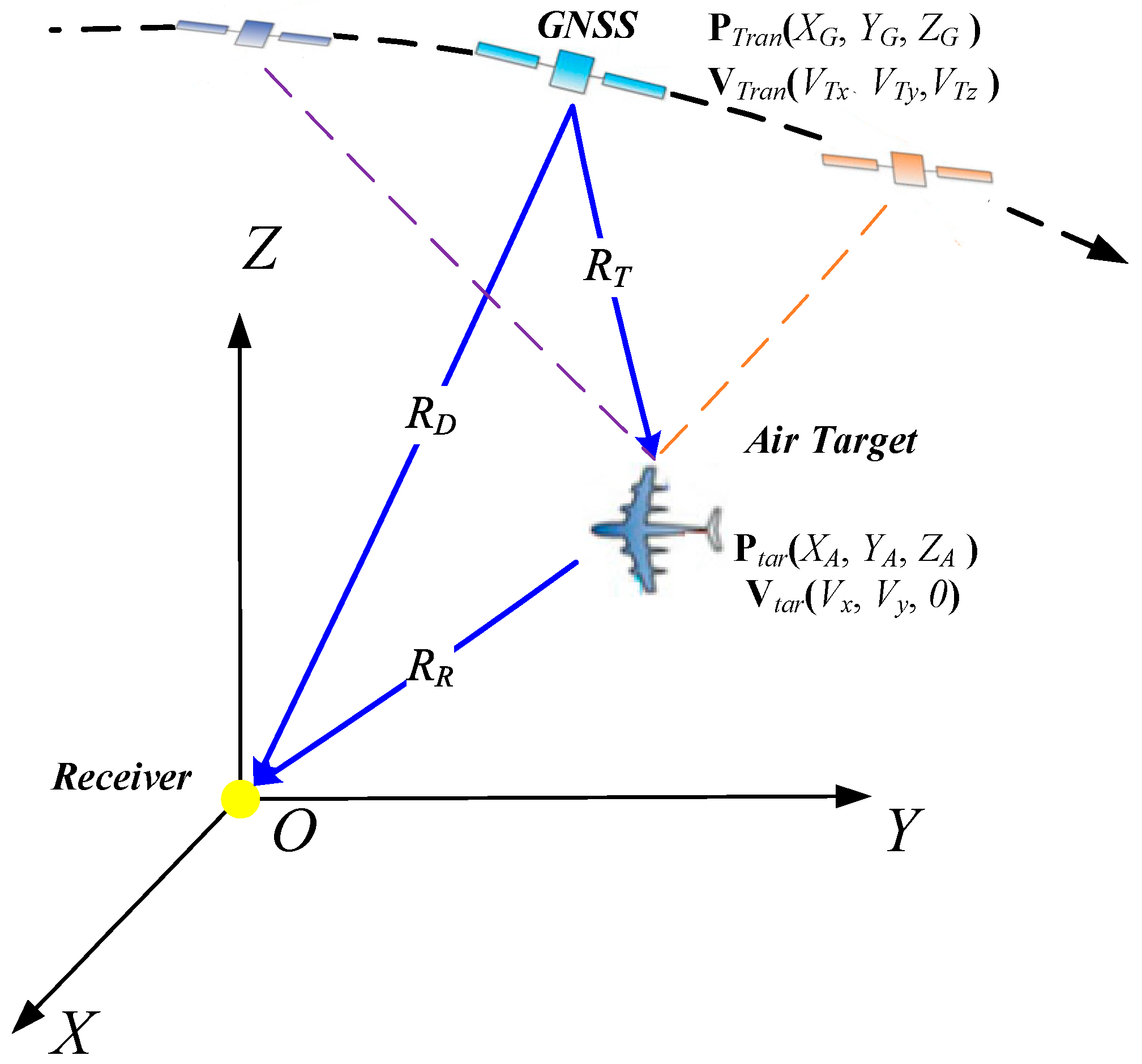
The air target detection geometric configuration of GNSS-based passive radar is shown in Figure 1, where the radar receiver is at the origin of the Cartesian coordinate system, while the X and Y axes point to the East and North directions, respectively. The air target is located at Ptar(XA,YA,ZA) and moves at a constant velocity Vtar(Vx, Vy, 0) and in a constant level. The GNSS transmitter is located at PTran(XG,YG,ZG) with a velocity vector VTran(VTx, VTy, VTz).
Based on the system geometry, the range history is the sum of the instantaneous receiver slant range RR(η) and transmitter slant range RT(η), which can be rewritten by Taylor series expansion.
where η, Rref, λ, fd, and fr denote the illumination time, reference range, signal wavelength, target Doppler centroid, and Doppler modulated rate, and fd and fr are derived as follows [36]:
where η = 0 means the illumination centroid time, fd0 and fr0 represent the Doppler centroid frequency and Doppler frequency modulated rate of the stationary target, and fd,v and fr,v are the corresponding variations caused by target motion. Besides, in GNSS-based passive radar, the reference signal, and its Doppler are also important for signal synchronization and range compression. As both the transmitter and the receiver co-ordinates are known, it is easy to remove the Doppler of reference signal from the synchronization outputs [14]. Therefore, to simplify the subsequent derivation, the Doppler of reference signal are not considered in this manuscript.
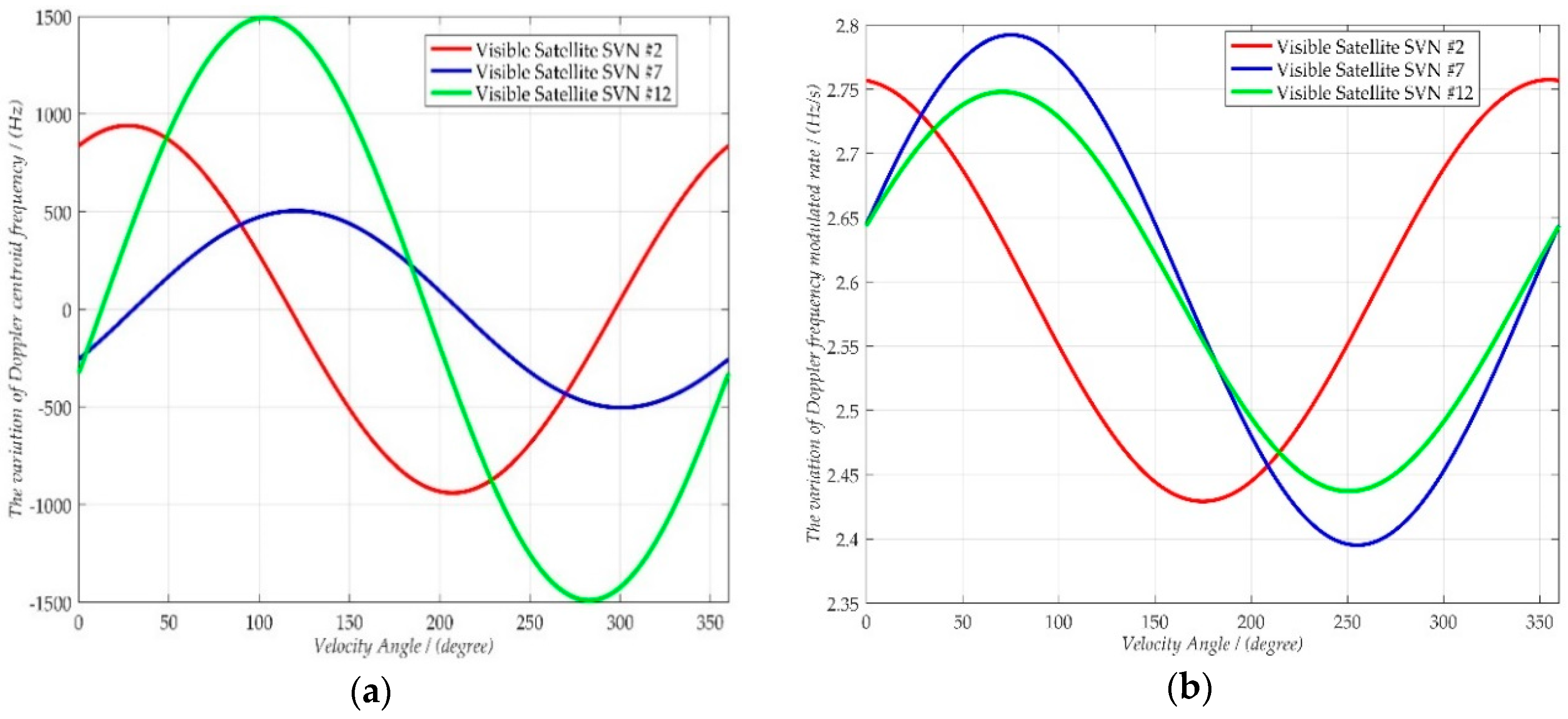
The additional unknown fd,v and fr,v will cause Doppler spectrum shift and image defocusing, which is a serious problem for long duration coherent integration processing and target detection. Assuming the air target is moving in the XOY plane with a velocity 220 m/s, Figure 2 shows the variations of fd,v and fr,v, using the parameters listed in Table 1. As shown in Figure 2, both fd,v and fr,v are greatly influenced by passive radar geometry and target motion direction. fd,v is mainly determined by the equivalent range velocity, and fr,v is mainly influenced by the equivalent azimuth velocity [36]. Normally, as depicted in Figure 2a, the range of fd,v is from −1500 Hz to 1500 Hz when the target velocity is smaller than 220 m/s (approximately 800 km/h). However, the pulse repetition frequency (PRF), fp, of the GNSS signal is 1000 Hz. As a result, the Doppler ambiguity phenomenon should be considered in the signal processing; otherwise, the blind speed will be inevitably detected. On the other side, fr,v is about 2.6 ± 0.2 Hz/s on this condition, which is relatively small because of the air target is far away from the receiver, and the corresponding range-curvature term is smaller than one range cell normally.
2.2. Air Target Echo Signal Model of GNSS-Based Passive Radar
In a GNSS system, the transmitted signal is a code-modulated continuous wave, the echo signal of GNSS-based passive radar forms a one-dimensional vector, and the target reflected GNSS signals from all visible satellites are received by the receiver antenna. According to [16], after quadrature demodulation, the target echo signal can be modeled as:
where superscript i represents using the i-th visible satellite as the transmitter, σ is the target radar cross-section, AT is the signal amplitude, Q(·) is the modulation code, and Tp, c, and λ denote signal period, speed of light, and signal wavelength, respectively. Then, set η = nTp + τ, tn = nTp, and the range history can be written as:
The Doppler frequency is also considered during the inter-period time, which is totally different with the traditional pulse radar. Besides, the second-term with inter-period time is ignored in (4).
Therefore, based on (4), the echo signal of GNSS-based passive radar can be rewritten in a 2-D form.
where the subscript n in tn is ignored for simplicity. As the transmitted code in each GNSS satellite is high-rate pseudo random noise (PRN) sequence, it has particularly excellent auto-correlation and cross-correlation properties, and these cross-correlation values are so small that they usually can be ignored. As a result, corresponding PRN code could not only be used as the matched filter but also be employed for separating the echo signal from different visible GNSS satellites. Hence, to simplify the subsequent derivation, one specific visible GNSS satellite is chosen as the transmitter, and the echo signal can be written as:
where Rref is the target reference range in center time, and the range-curvature in the envelop term is ignored, as it is much smaller than one range cell.
3. The Proposed 2-D Coherent Integration Processing and Target Detection Algorithm
Compared with the traditional radar signal, the signal power of GNSS is extremely weak. Consequently, to improve the performance of GNSS-based passive radar, not only the range integration gain, but also azimuth integration gain with long duration, must be obtained. In this section, a novel 2-D coherent integration algorithm is proposed, and based on this, a framework for aircraft target detection is presented. Firstly, the principle of RFT in introduced in Section 3.1. Then, the proposed algorithm is fully detailed in Section 3.2, with its fast implementation method and the target detection framework.
3.1. The Principle of RFT
For moving targets in radar applications, the echo signal after range compression s(t, r) is distributed on the range history line R(t) = v0t + r0, where r0 is the initial target position and v0 is target radial velocity. To coherently integrate the moving target’s azimuth echoes pulse by pulse, the traditional RFT for radar signal is by jointly searching range and velocity (r, v), which is [18]:
As Doppler frequency is fv = 2v/λ, the range history can be rewritten by R(t) = λfv0t/2 + r0, where fv0 is the target Doppler frequency. So, the RFT in the range-Doppler plane is:
Then, by defining the discrete searching range and Doppler parameters, the discrete form of traditional RFT has also been defined as [18]:
where Δr and Δfv are range and Doppler searching steps, rmin and fmin are the minimum target range and Doppler searching value, and Na, Nr, and Nf are the sample number of azimuth, range, and Doppler domains, respectively. As shown in (7)–(9), the RFT actually performs echo signal integration along a parameterized line defined by (r, v) or (r, fv). When the parameterized line (r0, v0) or (r0, fv0), coincides with the target range history, all echoes distributed on the line are integrated to a peak, and full coherent-integration gain processing is achieved.
In the traditional RFT, the Doppler rate or target high-order motion isn’t considered, and the monostatic radar is adopted. Then, the generalized RFT [28] has also been proposed using curvilinear integral for high-order motion detection, but higher dimensional parameter searching is needed, which is time and memory consuming.
3.2. Air Target Detection Based on 2-D Coherent Integration
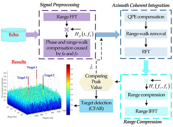
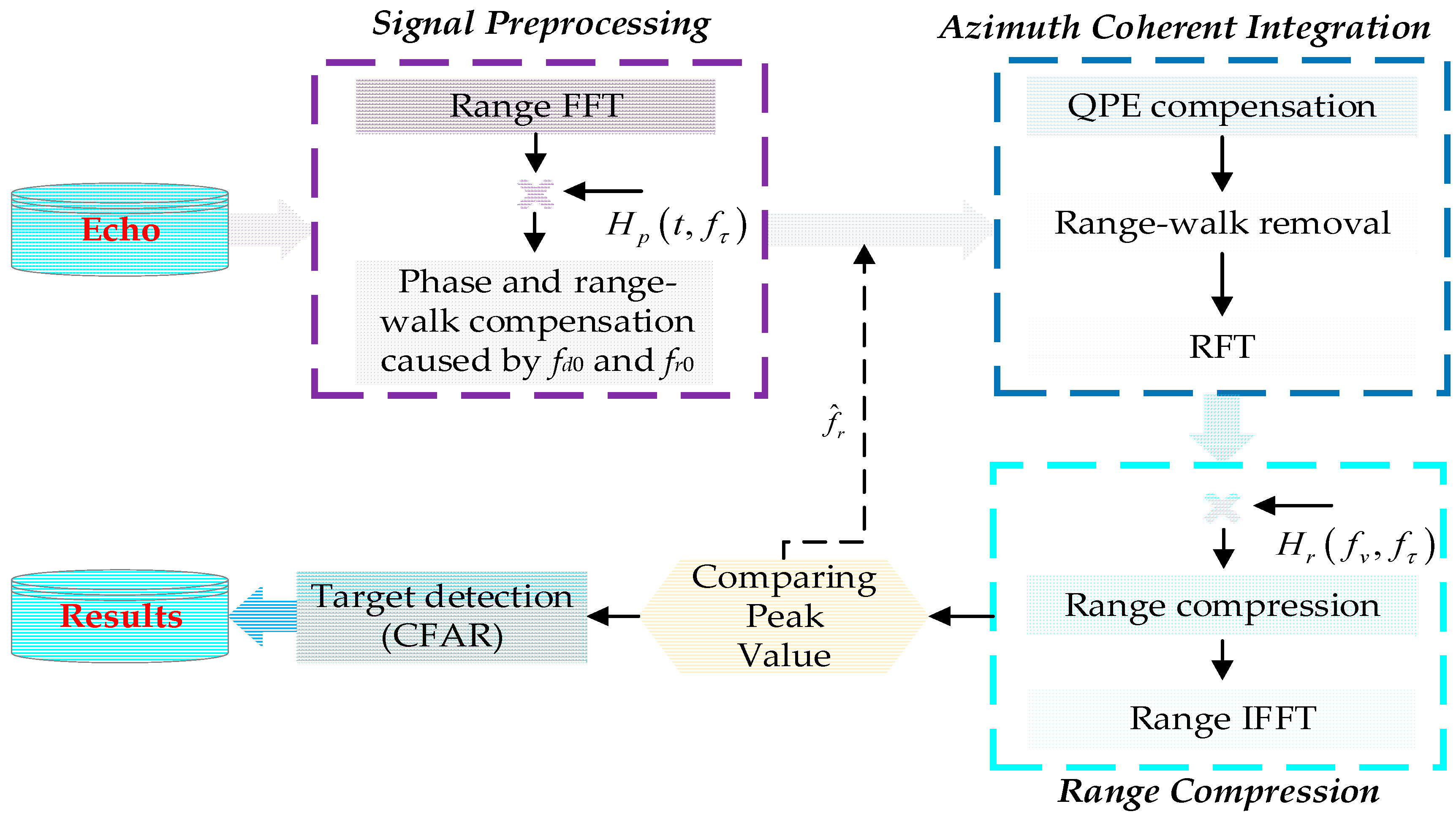
To guarantee the effectiveness and accuracy of air target detection, a sufficiently high SNR is crucial, which means long time illumination and 2-D coherent integration are needed. In the proposed novel air target detection algorithm, range-matched filtering and Doppler searching are combined to achieve the 2-D coherent-integration gain. Based on the deduced novel 2-D coherent integration algorithm, the framework of target detection using GNSS-based passive radar is shown in Figure 3, which mainly has four parts: The first is signal preprocessing to compensate the phase term and range-walk caused by the motion of GNSS satellite; the second is azimuth coherent integration processing with QPE compensation and range-walk removal; the third is range compression with a modified Doppler shift matched filter, after which the echo signal is totally focused on the range-Doppler plane; the last is air target detection based on the TAD or TBD method. The following provides details of the operations.
3.2.1. Signal Preprocessing
The signal preprocessing stage is performed to compensate the phase term and remove the range-walk, and both of them are caused by GNSS satellite’s motion. It starts with a range FFT to transform the echo signal into the range frequency domain, which is:
where Qf(·) is the FFT form of the GNSS modulation code,. Then, the phase term and range-walk caused by fd0 and fr0 are compensated with the 2-D filter .
In (11), the fd0 and fr0 are unknown, because the target position is unknown in advance. However, as the satellites orbit is about 20,000 km, the changing of slant range RT in different range cell is very small compared with the RT value itself. So, the difference of fd0 and fr0 in each position of the whole experiment scenario is quite small, and any range cell’s fd0 and fr0 is enough to guarantee the accuracy of 2-D filter in (11). In this situation, it is recommended to use the fd0 and fr0 in the scene center to construct the 2-D filter.
Then, the signal becomes:
3.2.2. Azimuth Coherent Integration
To obtain the coherent integration processing gain in azimuth, the principle of RFT is adopted at this stage. After the signal preprocessing, there is still residual quadratic phase error (QPE) caused by the unknown, fr,v, and residual range-walk term caused by the unknown, fd,v. For QPE estimation and compensation, many methods have been proposed in SAR imaging, and the simple and easy way is based on amplitude auto-focus method [37]. Besides, the residual range-walk can be removed by Doppler searching. Therefore, the azimuth coherent integration processing can be performed by QPE compensation, range-walk removal, and RFT, which is:
where
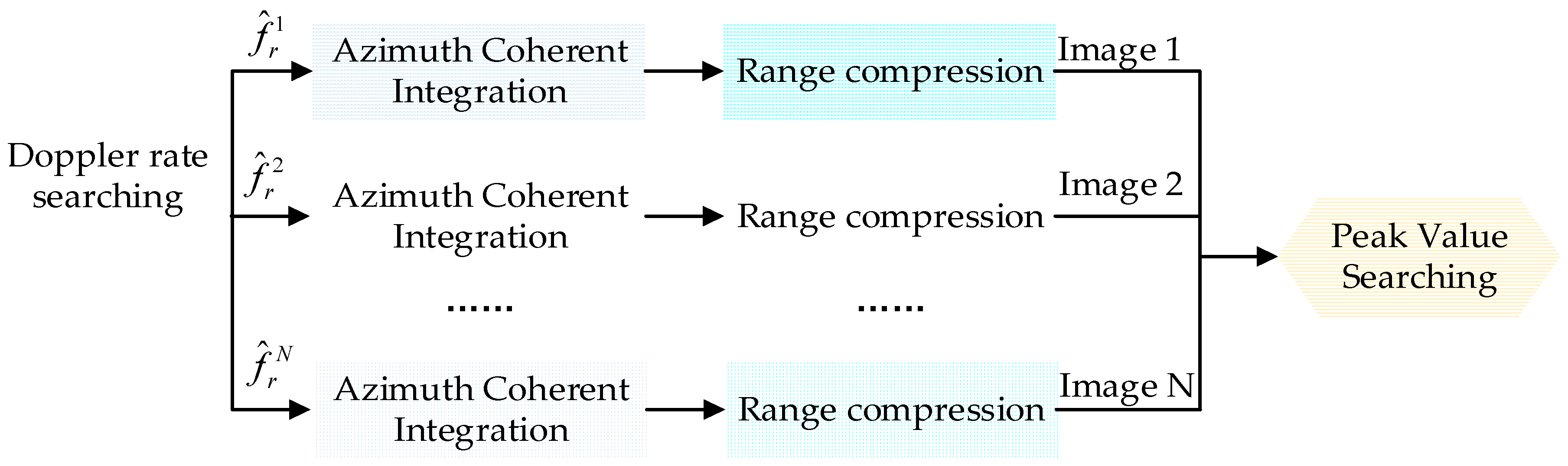
- The first phase term in the first line of Equation (13) is QPE compensation, and is the estimated Doppler rate parameter. As shown in Figure 2b, the variation range of Doppler rate is very small, and the maximum variation value is smaller than 0.6 Hz/s. Hence, we can use parallelized step search to estimate the Doppler rate (as shown in Figure 4), and this method has a high searching efficiency because of the small variation range of fr,v. Normally, the estimated Doppler rate can be expressed as:where , and denote the initial Doppler rate, Doppler rate searching step, and Doppler rate searching number, respectively. Finally, when matches the true value of target Doppler rate or equals zero, the azimuth coherent gain could be achieved and the maximum peak value of target will be obtained.
- The second phase term in the first line of Equation (13) is residual range-walk removal, and fv is the Doppler searching parameter. As shown in Equation (9), non-integer range cell is inevitable during the range history line searching, so range interpolation processing is necessary for traditional RFT. However, in Equation (13), when fv matches the target’s Doppler frequency, fd,v, all range-walk term is removed, and the echo signal will distribute along the line perpendicular to the range direction. Therefore, the non-interpolation processing is needed in the proposed algorithm, and the following azimuth integral processing is greatly simplified.
- The last phase term in the first line of Equation (13) is RFT processing, or called azimuth integral. As the range-walk term is removed, the echo signal is distributed along the azimuth direction. So, the RFT operation is similar to azimuth FFT operation.
Therefore, as shown in the azimuth integral in the second line of Equation (13), the azimuth coherent integration gain (see Equation (24)) is achieved when the Doppler searching parameter equals fd,v, the estimated Doppler rate equals fr,v, and the azimuth peak will occur at the target Doppler frequency point.
However, in Equation (13), the range-walk removal term is a three-dimensional filter, which means the whole azimuth coherent integration processing will have three nested loops in digital processing, and the computational complexity of this stage is o(NANRNV), where NA, NR, and NV denote azimuth sample number, range sample number, and Doppler searching number, respectively. Therefore, the azimuth coherent integration processing will take a lot of memory and increase the computational complexity. To improve the algorithm’s efficiency, a fast implementation of azimuth coherent integration based on the chirp-Z transform (CZT) [38] is presented in the following.
Firstly, we define the discrete series of searching Doppler frequency, azimuth time, and range frequency as:
where and denote Doppler searching step and range frequency cell, respectively. As shown in Figure 2a, the searching Doppler frequency is ambiguous, and the searching Doppler frequency series can be rewritten as:
where I and Nv denote the ambiguous Doppler index and non-ambiguous Doppler searching number. Based on this, Equation (13) can be rewritten as:
where
Then, using the principle of the CZT, we have:
where denotes the convolution operation. Besides, based on the relationship between convolution and FFT, Equation (19) can be performed in digital processing as:
where subscript m means the operation in the azimuth direction, DFTm(·) and IDFTm(·) denote the Discrete Fourier Transform and Inverse Discrete Fourier Transform, respectively.
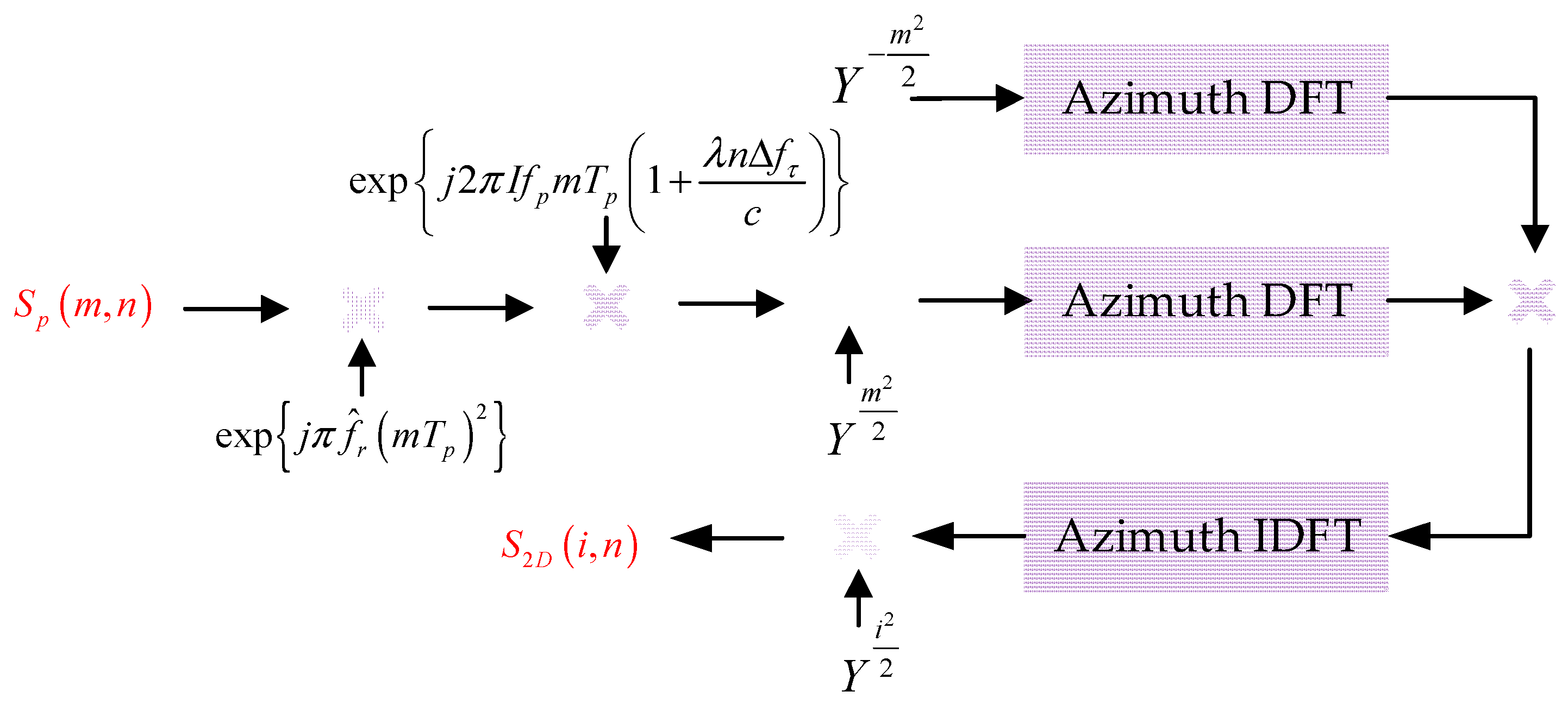
Actually, the calculation of (17) contains three nested loops (Doppler frequency, azimuth time, and range frequency), which is very memory and time consuming. But, as shown in (20) with CZT, the 3-D azimuth coherent integration processing is reduced to 2-D operation, and the computational complexity is o(NRNV), which is significantly lower than the 3-D processing. More details about computation complexity analysis can be seen in Chapter 4.2.4. Based on (20), the processing flow of azimuth coherent integration is shown in Figure 5.
3.2.3. Range Compression
After azimuth coherent integration processing, the target echo is focused in the Doppler domain. To maximize the signal-to-noise ratio and obtain fine range resolution of the sensed air target, range compression processing is performed. In tradition, the radar transmitted signal, like LFM, can be used as the matched filter for range compression. However, in GNSS-based passive radar, the transmitted PRN sequence is Doppler-intolerant, and a moving air target will introduce an unknown and non-negligible Doppler frequency fd,v. This will introduce a time-varying phase in the range direction and change the response of range compression. The traditional cross-ambiguity function could be used for range compression with Doppler and range 2-D joint-searching in each signal period [20,21,22]. But it will very time consuming because of the extremely long azimuth coherent time. Therefore, a special matched filter including Doppler frequency is necessary.
Normally, the matched filter is generated by the reference signal. In this manuscript, the Doppler of the reference signal is ignored, because it is easy to remove with a known baseline range history [14]. Besides, the phase errors caused by atmospheric propagation and clock slippage are also ignored, because those errors in reference signal and target signal can be modelled as having the same error, and they are easily removed after range compression [14].
The signal after azimuth coherent integration is transformed into the 2-D frequency domain, so the modified matched filter can be modeled easily in the 2-D frequency domain, and a shifting Doppler in each Doppler line is included.
where subscript τ means the FFT operation in the fast time direction. By multiplying the modified matched filter and performing range IFFT operation, the signal after 2-D coherent processing is:
where the superscript * represents the complex conjugate of . Then, let , and replacing the azimuth time integral with summation, the final result can be expressed as:
where QC is the gain of range compression, normally QC equals Bw/fp, and Bw is the signal bandwidth. D(·) is the normalized envelope of the auto-correlation result of GNSS transmitted signal, and D(0) = 1. is the factor caused by mismatched Doppler frequency in range compression, and , which means the range compression is matched filtering when . Here, as shown in Figure 4, we use parallelized search to estimate the Doppler rate. Then, when the error of estimated Doppler rate is zero, the signal is:
where azimuth sample number, NA, equals coherent time multiplied by the signal repetition rate, and NA is the azimuth coherent integration. Considering the geometry of GNSS-based passive radar, each moving target’s range Doppler parameters are totally different. Therefore, even in multi-targets case, all targets are focused at their own Doppler parameter position.
Clearly, the maximum value will occur at the position of target motion parameter . Therefore, by comparing the peak value of the processing result with different estimated Doppler rate,, the coherent integration gain can be achieved after the 2-D coherent integration processing.
3.2.4. Target Detection
After the 2-D coherent integration processing, the air target is focused on the range-Doppler plane. Apart from the target’s signal, the system noise and clutter also exist in the focused range-Doppler data. Therefore, target detection is performed to obtain the air target’s motion parameters. Normally, the likelihood ratio function (LRF) is used for target detection, and many methods based on LRF have been presented, which can be divided into two categories: Tracking and detection (TAD), and track before detection (TBD) [34,35]. In TAD, the constant false alarm detection (CFAR) is typically used, and to obtain the detection probability of 80% with a constant false alarm probability 10−6 in the additive white Gaussian noise background, the minimum signal-to-noise ratio (SNR) is 12.8 dB [18]. In TBD, the particle filter (PF) is commonly used, and it is capable of detecting a moving target with SNR as low as 7 dB [35]. In this paper, the CFAR method is used in the target detection part.
4. Experiments and Discussion
To demonstrate the performance of the proposed algorithm and the feasibility of target detection using GNSS-based passive radar, numerical simulations including comparison experiments and multi-static experiments are carried out in Section 4.1. Then, based on the results, the performance of GNSS-based passive radar and the proposed algorithm is discussed in Section 4.2, which mainly has three parts: System power budget analysis and available coherent time for aircraft target detection, best choice of the Doppler rate searching step, and processing performance when Doppler ambiguity exists.
4.1. Experiments and Results
In the experiments, the newly modernized civil signal GPS L5 is adopted, as it is at least ten times wider in signal bandwidth and four times stronger in terms of signal power than traditional civil signal GPS L1 [39,40]. Hence, both of signal bandwidth and signal power are beneficial to aircraft detection, and GPS L5 is a superior option in GNSS-based passive radar. The motion parameters of three targets and the associated simulation parameters are listed in Table 1. First, a comparison between the tradition RFT and the proposed algorithm is presented to verify the validity of the proposed algorithm. Then, multi-satellites (three satellites) joint experiments are presented for aircraft detection and motion parameters estimation.
4.1.1. Comparing Results Using the Proposed Algorithm and Traditional RFT
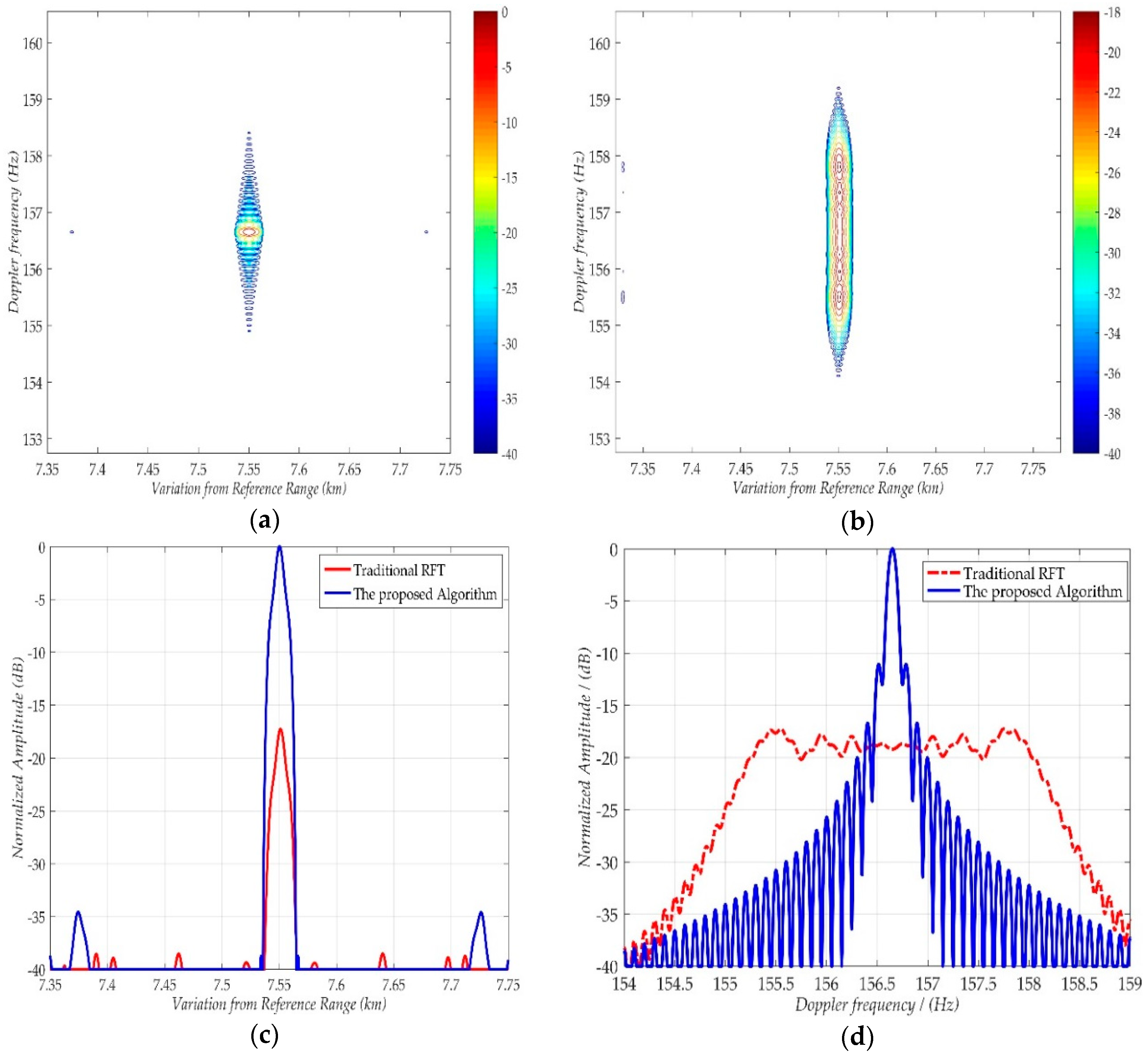
To illustrate the performance and feasibility of the proposed 2-D coherent processing algorithm, the processing results of target-3 with traditional RFT [18] and our proposed algorithm are shown in Figure 6. GPS SVN #7 is used as the transmitter, and noise is not considered in echoes. As shown in Figure 6b,d, the processing result using the traditional RFT is totally defocused in the Doppler dimension, as the residual QPE (Doppler rate term) caused by the motion of target. Besides, energy loss exists after range compression, as shown in Figure 6c, because the range match filter in traditional RFT is mismatched for an unknown non-zero Doppler frequency. For the proposed 2-D coherent processing algorithm, both Doppler and range profile are accurately focused as shown in Figure 6a. Furthermore, as listed in Table 2, the peak of them is equal to target’s Doppler and range parameters, and the accuracy is better than one Doppler searching or range bin. Thus, the proposed method has a good performance on moving target focusing.
4.1.2. Multi-Static Experiments and Aircrafts Motion Parameters Estimation
Due to the abundance of GNSS signal resources, multi-angle illumination from over 20 satellites in any given area is attainable. So, multi-satellite (SVN #2, #7, and #12) joint experiments are carried out to verify the applicability and generality of the proposed 2-D coherent processing and target detection method. With different geometries for those three transmitters, each target’s Doppler and range parameters are totally different. Even the same target’s Doppler and range parameters are changed with different transmitters. All motion parameters of those three targets are listed in Table 2. According to the power budget, those three targets’ ideal SNRs are 13.6, 13.8, and 13.9 dB, respectively. By applying the proposed 2-D coherent processing algorithm, those three targets are well-focused as demonstrated in Figure 7, and their measured SNR is 13.5, 13.6 and 13.8 dB respectively. The energy loss is mainly because of the residual estimated Doppler rate. Even so, the energy loss is small enough and acceptable. Then, based on the 2-D focused result in the range-Doppler plane, target detection experiments are carried out with the CFAR method, and the detection results are listed in Table 2. As shown, all targets have been detected and accurately estimated Doppler and range parameters are obtained.
The connection between a target’s location, velocity, and range Doppler parameters is:
where the functions F(·) and G(·) are determined by (1) and (2), respectively. According to (25), it is impossible to achieve a target’s location and velocity with only a group of range Doppler parameters. Fortunately, as shown in Figure 7 and Table 2, a set of different range Doppler parameters could be achieved with each available GNSS satellite. Therefore, multi-element nonlinear equations can be obtained by using several satellites (at least three to obtain the target’s 3-D motion parameters). Finally, as listed in Table 3, all targets’ locations and velocities are estimated accurately.
4.2. Discussion
4.2.1. Power Budget and Coherent Time
The system thermal noise always exists in the radar echo signal, and, according to the radar function, the SNRin of echo signal is:
where PE is the GNSS signal power near the Earth’s surface, and it equals −154 dB in GPS L5 signal case [40]; GR is the antenna gain of receiver, and it is set to 35 dB as listed in Table 1; σ is target RCS, for a medium-sized aircraft (like Boeing 737–400), its RCS exceeds 20 dB in L-band, and in some azimuth angle, the RCS is larger than 26 dB [41]; RR is the range between target and receiver, k is the Boltzmann constant, Ts is system Kelvin temperature, Bw is the signal bandwidth, and FnL is system noise coefficient. For GNSS-based passive radar with the GPS-L5 signal, SNRin is roughly smaller than −70 dB. Hence, the 2-D coherent integration gain is necessary to obtain a sufficiently high SNR for target detection.
After the 2-D coherent integration processing, the azimuth and range processing gain is achieved, and the SNRo of processing result is:
where Tc is the coherent time, TpBw and fpTc are the range and azimuth processing gain, respectively. Normally, to guarantee the effectiveness of target detection, the minimum SNR (SNRmin) of the processing results should be obtained. So, the coherent time, Tc, needs to be longer than the lower bound, which is:
Furthermore, during the derivation of the proposed algorithm, the assumption that the range-curvature term is less than half range resolution bin is considered. In GNSS-based passive radar, the best range resolution we can have is c/2Bw in the quasi-monostatic case, and the range-curvature term is . So, this assumption determines the upper bound of coherent time Tc, which is:
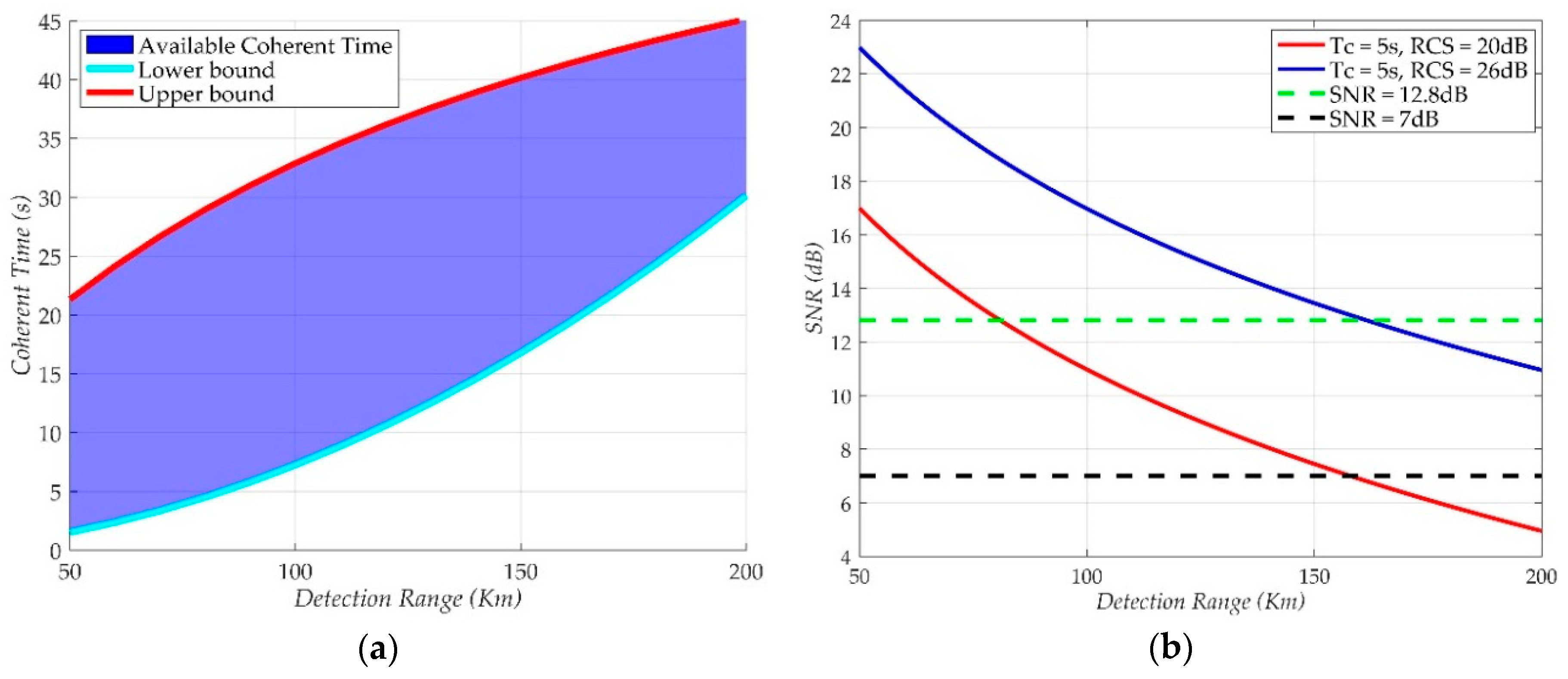
Based on the upper bound and lower bound of the coherent time, Figure 8a has shown the available coherent time for aircraft detection in GNSS-based passive radar, with the parameters listed in Table 1 and SNRmin equal to 12.8 dB. Then, with coherent time Tc equal to 5 s, the result of power-budget analysis is shown in Figure 8b. As shown, the detection range of aircraft using GNSS-based passive radar is larger than 80 km, and it will be increased twofold in the RCS enhancement area. Furthermore, with the advanced target detection method, like TBD, the detection range can easily reach 200 km, as shown in Figure 8b.
4.2.2. Searching Step of Doppler Rate
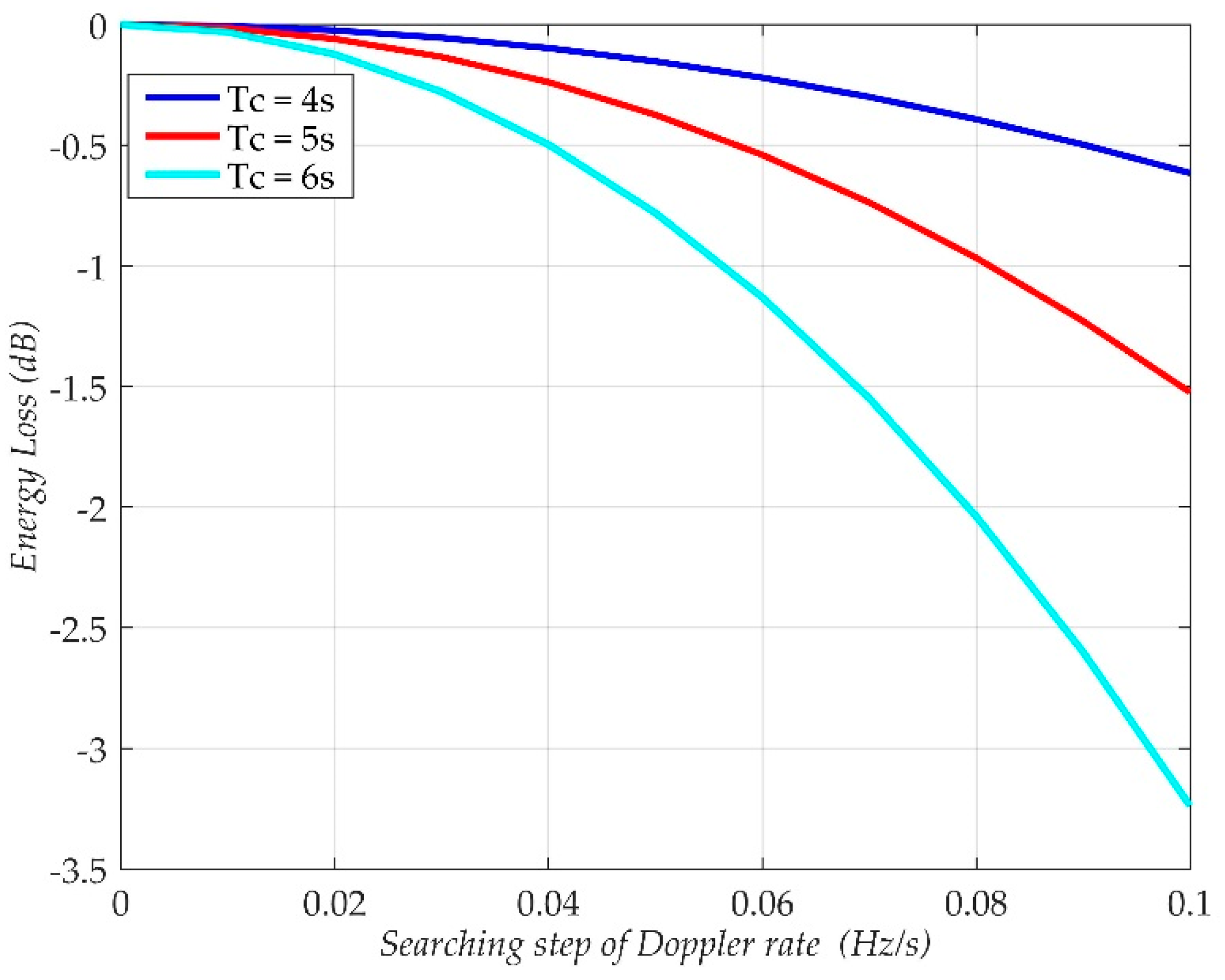
In (23), the residual quadratic phase error still exists because of the error of estimated Doppler rate , and it mainly depends on the searching step of Doppler rate . Generally, the smaller searching step we choose, the smaller the error of estimated Doppler rate. However, choosing a small searching step means the searching number is accordingly increasing, which will significantly increase the computational load. Therefore, choosing the parameter is very important in the proposed algorithm.
Due to the error , the 2-D coherent integration gain is reduced, and the energy loss at the position of target motion parameters (fd,v, Rref) is:
Based on (30), with the parameters listed in Table 1, Figure 9 shows the impact of searching step on the energy loss of the final processing results. In Figure 9, as the searching step increases, the energy loss will increase significantly. In our case (Tc is 5 s), the energy loss (less than 0.2 dB) could be ignored when is 0.04 Hz/s. Besides, the variation of fr,v is smaller than 0.4 Hz/s, as shown in Figure 2b, and as a result, the maximum searching number is only 10, which is absolutely acceptable.
4.2.3. Doppler Ambiguity
According to the analysis in Section 2.1, the Doppler frequency fd,v varies from −1500 Hz to 1500 Hz. Therefore, the range of searching Doppler frequency is [−1500, 1500] Hz, and the Doppler ambiguity is inevitable because fp of the GNSS signal is 1000 Hz. Let the ambiguous Doppler frequency be:
where is the ambiguous Doppler frequency, and I is the ambiguous Doppler index. So, the range and Doppler profiles of the final coherent integration processing result can be written as:
where the residual quadratic phase term has been ignored. With the parameters listed in Table 1, the interpolated range and Doppler profiles are shown in Figure 10. As shown, energy loss exists in the range dimension, and the final result cannot be focused in the range-dimension, because of the ambiguous Doppler frequency. To evaluate the impact of Doppler ambiguity, the blind Doppler sidelobe ratio (BDSR) can be defined as:
where I is equal to ±1, ±2. When the coherent time is 5 s, NA = 5000, BDSR(±1) = −17.06 dB, and BDSR(±2) = −27.40 dB. As the BDSR is very low, the blind Doppler sidelobe will submerge in the noisy background. Therefore, both the range/Doppler profile and BDSR results demonstrate that the proposed algorithm has a good performance even in the Doppler ambiguity situation, and the problem of blind speed is also overcome.
4.2.4. Computation Analysis about the Azimuth Coherent Processing
In GNSS-based passive radar, the long coherent time is needed and the range Doppler searching is implemented. So, the azimuth coherent processing could be time-consuming. In this section, the computation complexity analysis is given.
In digital processing case, one complex multiplication needs six floating-point (FLOP) operations, and the signal FFT and IFFT operation with a length of N needs 5Nlog2(N) FLOP. Therefore, based on (13) and (17), the azimuth processing computation load is:
Then, the fast implementation method based on CZT for azimuth coherent processing is presented. According to (20), the fast azimuth processing computation load is:
Assume that the computational efficiency γ is defined as C1/C2. Normally, we let NV = NA, and with the condition of the same parameters as listed in Table 1, the computational efficiency γ is:
Therefore, the computational complexity of the proposed method is significantly reduced by the CZT operation.
5. Conclusions
GNSS-based passive radar is a useful tool to detect aircrafts, because of its system advantages and signal characteristics. According to the power budget analysis, the detection range of aircrafts is ranging from 80 km to 150 km, and it can still be improved if advanced moving target detector is adopted. However, during the echo signal processing, there are great challenges to achieve coherent integration gain in both range and azimuth dimensions, which will limit the performance of GNSS-based passive radar significantly.
Therefore, a novel 2-D coherent integration processing and detecting algorithm is proposed for aircraft detection. In this paper, a modified RFT with range-walk removal and Doppler rate estimation is performed for azimuth long time coherent processing, and its fast implementation method based on the Chirp-Z transform is also presented. Furthermore, a modified matched filter with a shifting Doppler frequency in each Doppler line is performed for range compression. Hence, 2-D coherent integration gain is obtained, and the range-Doppler focused result has a sufficiently high SNR for detection. The excellent performance of the proposed algorithm is demonstrated by numerical simulation experiments. Moreover, as the experimental results shown, the blind Doppler sidelobes are weak enough to submerge in the noise background, which demonstrate that the proposed algorithm has good performance even when Doppler ambiguity exists. With the estimated motion parameters of the aircraft, the aircraft image could be obtained by GNSS-based SAR imaging formation algorithm. Although the fast implementation method based on CZT is used in the azimuth coherent processing, the computation load of the proposed algorithm is still large because of the long coherent time. Therefore, in real-data experiments, parallel computing based on FPGA or GPU is highly recommended.
Although GNSS signals give low power density at the aircraft targets, their abundance and the variety of geometric configurations from different satellites provide two major advantages: (1) The bistatic angle giving largest RCS can be selected to improve the radar detection range; (2) the multiple observation geometries allow the algorithm to obtain not only the range and Doppler parameters of aircraft but also its position and velocity. Therefore, based on experiments and power budget analysis, this paper has also highlighted the potential of GNSS-based passive radar as an assistive tool for air traffic control.
The near future work in this direction is to test the proposed algorithm with real GNSS-based passive radar echo signals. Later work will explore aircraft target detection and tracking in low SNR, as this could dramatically increase the GNSS-based passive radar’s range of coverage.
Author Contributions
H.-C.Z. and P.-B.W. implemented the methods and conceived and designed the experiments; H.-C.Z. and W.Y. performed the experiments and analyzed the data; J.C. and W.L. supervised the research; and H.-C.Z. wrote the paper.
Funding
This research received no external funding.
Acknowledgments
This work is supported by the International S&T Cooperation Program of China (ISTCP) under Grant No. 2015DFA10270, and the National Science Foundation of China (NSFC) under Grant No. 61671043.
Conflicts of Interest
The authors declare no conflict of interest.
Appendix A. Delay-Doppler Ambiguity Function of GNSS and LFM Signal
In radar system, the properties of the transmitted waveform determines the range and Doppler resolution, and the delay-Doppler ambiguity function is usually used to evaluate these properties [42], which is:
where S(t) is the directly received transmitted signal, r, 2r/c, and fD denote the range, time delay, and Doppler frequency, respectively.
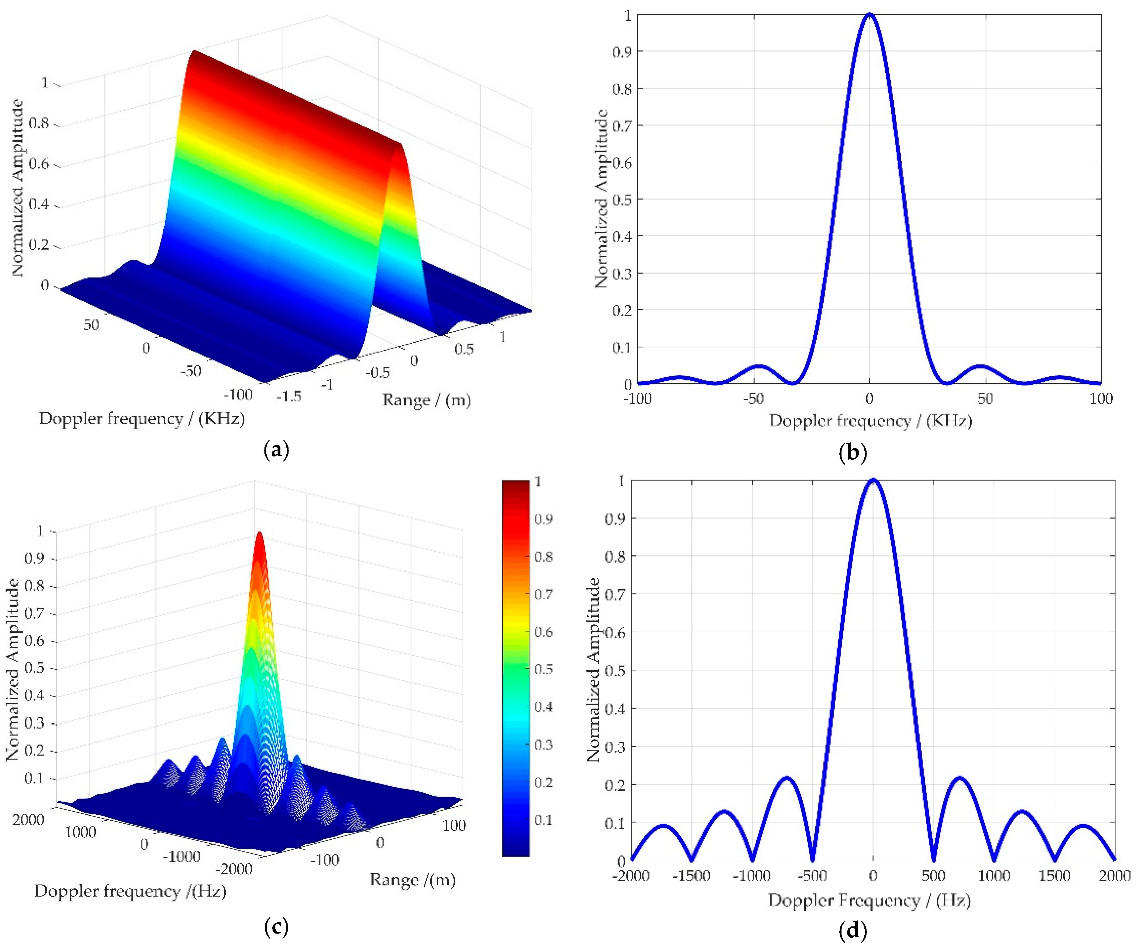
Based on (A1), Figure A1 shows the delay-Doppler ambiguity function for LFM signal (bandwidth: 300 MHz, pulse width: 30 µs) and GPS-L5 signal (bandwidth: 20.46 MHz, signal width: 1 ms). In LFM signal, we can see that the main-lobe is part of a delay-Doppler ridge that exhibits a gradual roll-off from the peak, and an appreciable Doppler shift induces a little SNR loss relative to the peak value. So, the LFM signal is also called a Doppler-tolerant waveform [42]. However, as shown in Figure A1c,d, totally different with traditional LFM, the peak of the autocorrelation of the GPS-L5 only appears at (r = 0, fD = 0), and even a small Doppler shift will lead to large SNR loss. Therefore, we can define that the GNSS signal is Doppler-intolerant. For airplane target detection, the range of target Doppler frequency is from −1500 Hz to 1500 Hz (shown in Figure 2), and the big Doppler shift is obviously not negligible, which means the Doppler frequency should be considered during the range compression processing.
Figure A1.
Delay-Doppler ambiguity function of LFM and GPS-L5 signal. (a) Three-dimensional results of LFM (b) Doppler frequency profile of LFM (c) Three-dimensional results of GPS-L5 (d) Doppler frequency profile of GPS-L5.
Figure A1.
Delay-Doppler ambiguity function of LFM and GPS-L5 signal. (a) Three-dimensional results of LFM (b) Doppler frequency profile of LFM (c) Three-dimensional results of GPS-L5 (d) Doppler frequency profile of GPS-L5.

Appendix B
The derivation of (13) is as follows:
where is the residual error between the true value, fr,v, and the estimated value, .
References
- Del-Rey-Maestre, N.; Mata-Moya, D.; Jarabo-Amores, M.; Gómez-del-Hoyo, P.; Bárcena-Humanes, J.; Rosado-Sanz, J. Passive Radar Array Processing with Non-Uniform Linear Arrays for Ground Target’s Detection and Localization. Remote Sens. 2017, 9, 756. [Google Scholar] [CrossRef]
- Shang, H.; Jia, L.; Menenti, M. Modeling and reconstruction of time series of passive microwave data by discrete Fourier transform guided filtering and harmonic analysis. Remote Sens. 2016, 8, 970. [Google Scholar] [CrossRef]
- Belfiori, F.; Monni, S.; Rossum, W.V.; Hoogeboom, P. Antenna array characterisation and signal processing for an FM radio-based passive coherent location radar system. IET Radar Sonar Navig. 2012, 6, 687–696. [Google Scholar] [CrossRef]
- Colone, F.; Faclone, P.; Bongioanni, C.; Lombardo, P. WiFi-based passive bistatic radar: Data processing schemes and experimental results. IEEE Trans. Aerosp. Electron. Syst. 2012, 48, 1061–1079. [Google Scholar] [CrossRef]
- Ribo, S.; Arco, J.C.; Oliveras, S.; Cardellach, E.; Rius, A.; Buck, C. Experimental results of an X-band PARIS reciver using digital satellite TV opportunity signals scattered on the sea surface. IEEE Trans. Geosci. Remote Sens. 2014, 52, 5704–5711. [Google Scholar] [CrossRef]
- Ma, H.; Antoniou, M.; Pastina, D.; Santi, F.; Pieralice, F.; Bucciarelli, M.; Cherniakov, M. Maritime Moving Target Indication Using Passive GNSS-based Bistatic Radar. IEEE Trans. Aerosp. Electron. Syst. 2018, 54, 115–130. [Google Scholar] [CrossRef]
- Clemente, C.; Soraghan, J.J. GNSS-Based Passive Bistatic Radar for Micro-Doppler Analysis of Helicopter Rotor Blades. IEEE Trans. Aerosp. Electron. Syst. 2014, 50, 491–500. [Google Scholar] [CrossRef]
- Liu, F.; Antoniou, M.; Zeng, Z.; Cherniakov, M. Coherent change detection using passive GNSS-based BSAR: Experimental proof of concept. IEEE Trans. Geosci. Remote Sens. 2013, 51, 4544–4555. [Google Scholar] [CrossRef]
- He, X.; Zeng, T.; Cherniakov, M. Signal detectability in SS-BSAR with GNSS non-cooperative transmitter. IEE Proc. Radar Sonar Navig. 2005, 152, 124–132. [Google Scholar] [CrossRef]
- Hu, C.; Liu, C.; Wang, R.; Chen, L.; Wang, L. Detection and SISAR Imaging of Aircrafts Using GNSS Forward Scatter Radar: Signal Modeling and Experimental Validation. IEEE Trans. Aerosp. Electron. Syst. 2017, 53, 2077–2093. [Google Scholar] [CrossRef]
- Suberviola, I.; Mayordomo, I.; Mendizabal, J. Experimental Results of Air Target Detection with a GPS Forward-Scattering Radar. IEEE Geosci. Remote Sens. Lett. 2011, 9, 47–51. [Google Scholar] [CrossRef]
- Kabakchiev, C.; Garvanov, I.; Behar, V.; Kabakchieva, D.; Kabakchiev, K.; Rohling, H.; Kulpa, K.; Yarovoy, A. Detection and classification of objects from their radio shadows of GPS signals. In Proceedings of the 2015 16th International Radar Symposium (IRS), Dresden, Germany, 24–26 June 2015; pp. 906–991. [Google Scholar]
- Glennon, E.P.; Dempster, A.G.; Rizos, C. Feasibility of Air Target Detection Using GPS as a Bistatic Radar. J. Glob. Position. Syst. 2006, 5, 119–126. [Google Scholar] [CrossRef] [Green Version]
- Antoniou, M.; Cherniakov, M. GNSS-based bistatic SAR: A signal processing view. Eurasip J. Adv. Signal Process. 2013, 1, 1–16. [Google Scholar] [CrossRef]
- Ma, H.; Antoniou, M.; Cherniakov, M. Passive GNSS-Based SAR Resolution Improvement Using Joint Galileo E5 Signals. IEEE Geosci. Remote Sens. Lett. 2015, 12, 1640–1644. [Google Scholar] [CrossRef]
- Zeng, H.; Wang, P.; Chen, J.; Liu, W.; Ge, L. A Novel General Imaging Formation Algorithm for GNSS-Based Bistatic SAR. Sensors 2016, 16, 1–15. [Google Scholar] [CrossRef] [PubMed]
- Tao, R.; Zhang, N.; Wang, Y. Analysing and compensating the effects of range and Doppler frequency migrations in linear frequency modulation pulse compression radar. IET Radar Sonar Navig. 2011, 5, 12–22. [Google Scholar] [CrossRef]
- Xu, J.; Yu, J.; Peng, Y.N.; Xia, X.G. Radon-Fourier transform for radar target detection, I: Generalized Doppler filter bank. IEEE Trans. Aerosp. Electron. Syst. 2011, 47, 1186–1202. [Google Scholar] [CrossRef]
- Giangregorio, G.; Bisceglie, M.; Addabbo, P.; Beltramonte, T.; D’Addio, S.; Galdi, C. Stochastic modeling and simulation of Delay-Doppler Maps in GNSS-R over the ocean. IEEE Trans. Geosci. Remote Sens. 2016, 54, 2056–2069. [Google Scholar] [CrossRef]
- Colone, F.; Langellotti, D.; Lombardo, P. DVB-T signal ambiguity Function Control for Passive Radars. IEEE Trans. Aerosp. Electron. Syst. 2014, 50, 329–347. [Google Scholar] [CrossRef]
- Howland, P.E.; Maksimiuk, D.; Reitsma, G. FM radio based bistatic radar. IET Radar Sonar Navig. 2005, 152, 107–115. [Google Scholar] [CrossRef]
- Saini, R.; Cherniakov, M. DTV signal ambiguity function analysis for radar application. IET Radar Sonar Navig. 2005, 152, 133–142. [Google Scholar] [CrossRef]
- Skolnik, M.; Linde, G.; Meads, K. Senrad: An advanced wideband air-surveillance radar. IEEE Trans. Aerosp. Electron. Syst. 2011, 37, 1163–1175. [Google Scholar] [CrossRef]
- Perry, R.P.; Dipietro, R.C.; Fante, R.L. Coherent integration with range migration using Keystone formatting. In Proceedings of the IEEE Radar Conference, Boston, MA, USA, 17–20 April 2007; pp. 863–868. [Google Scholar]
- Li, G.; Xia, X.G.; Peng, Y.N. Doppler Keystone Transform: An Approach Suitable for Parallel Implementation of SAR Moving Target Imaging. IEEE Geosci. Remote Sens. Lett. 2008, 5, 573–577. [Google Scholar] [CrossRef]
- Huang, P.; Liao, G.; Yang, Z.; Xia, X.G.; Ma, J.T.; Zheng, J.B. Ground Maneuvering Target Imaging and High-Order Motion Parameter Estimation Based on Second-Order Keystone and Generalized Hough-HAF Transform. IEEE Trans. Geosci. Remote Sens. 2017, 55, 320–335. [Google Scholar] [CrossRef]
- Satzoda, R.K.; Suchitra, S.; Srikanthan, T. Parallelizing the Hough transform computation. IEEE Signal Process. Lett. 2008, 15, 297–300. [Google Scholar] [CrossRef]
- Xia, J.W.; Zhou, Y.; Jin, X.; Zhou, J.J. A Fast Algorithm of Generalized Radon-Fourier Transform for Weak Maneuvering Target Detection. Int. J. Antennas Propag. 2016, 1–10. [Google Scholar] [CrossRef]
- Xu, J.; Yu, J.; Peng, Y.N.; Xia, X.G.; Long, T. Space–time Radon–Fourier transform and applications in radar target detection. IET Radar Sonar Navig. 2012, 6, 846–857. [Google Scholar] [CrossRef]
- Xu, J.; Yan, L.; Zhou, X.; Xia, X.G.; Long, T.; Wang, Y.; Farina, A. Adaptive Radon-Fourier Transform for Weak Radar Target Detection. IEEE Trans. Aerosp. Electron. Syst. 2018, 1. [Google Scholar] [CrossRef]
- Xu, J.; Yu, J.; Peng, Y.N.; Xia, X.G. Radon-Fourier Transform for Radar Target Detection, II: Blind Speed Sidelobe Suppression. IEEE Trans. Aerosp. Electron. Syst. 2011, 47, 2473–2486. [Google Scholar] [CrossRef]
- Chen, X.L.; Guan, J.; Liu, N.B.; He, Y. Maneuvering Target Detection via Radon-Fractional Fourier Transform-Based Long-Time Coherent Integration. IEEE Trans. Signal Process. 2014, 62, 939–953. [Google Scholar] [CrossRef]
- Cheng, Y.; Bao, Z.; Zhao, F.; Lin, Z. Doppler compensation for binary phase-coded waveforms. IEEE Trans. Aerosp. Electron. Syst. 2011, 38, 1068–1072. [Google Scholar] [CrossRef]
- Robey, F.C.; Fuhrmann, D.R.; Nitzberg, R.; Kelly, E.J. A CFAR adaptive matched filter detector. IEEE Trans. Aerosp. Electron. Syst. 1992, 28, 208–216. [Google Scholar] [CrossRef]
- Gao, H.; Li, J.W. Detection and Tracking of a Moving Target Using SAR Images with the Particle Filter-Based Track-Before-Detect Algorithm. Sensor 2014, 14, 10829–10845. [Google Scholar] [CrossRef] [PubMed] [Green Version]
- Yang, W.; Chen, J.; Liu, W.; Wang, P.B. Moving Target Azimuth Velocity Estimation for the MASA Mode Based on Sequential SAR Images. IEEE J.-STARS 2017, 10, 2780–2790. [Google Scholar] [CrossRef]
- Cumming, I.G.; Wong, F.H. Digital Processing of Synthetic Aperture Radar Data: Algorithm and Implementation; Artech House: Boston, MA, USA, 2005; pp. 380–390. [Google Scholar]
- Yu, J.; Xu, J.; Peng, Y.N.; Xia, X.G. Radon-Fourier Transform for Radar Target Detection, III: Optimality and Fast Implementations. IEEE Trans. Aerosp. Electron. Syst. 2012, 48, 991–1004. [Google Scholar] [CrossRef]
- Zeng, H.; Chen, J.; Zhang, H.; Yang, W.; Wang, P. A modified imaging formation algorithm for bistatic SAR based on GPS-L5 signal. In Proceedings of the 2017 IEEE International Geoscience and Remote Sensing Symposium (IGARSS), Fort Worth, TX, USA, 23–28 July 2017; pp. 4129–4132. [Google Scholar]
- Behar, V.; Kabakchiev, C. Detectability of Air Targets using Bistatic Radar Based on GPS L5 Signals. Int. Radar Symp. 2011, 7–9, 212–217. [Google Scholar]
- Sukharevsky, O.I. Electromagnetic Wave Scattering by Aerial and Ground Radar Objects; Taylor & Francis Group, CRC Press: Boca Raton, FL, USA, 2015; pp. 162–174. [Google Scholar]
- Blunt, S.D.; Mokole, E.L. Overview of Radar Waveform Diversity. IEEE Aerosp. Electron. Syst. Mag. 2016, 31, 2–42. [Google Scholar] [CrossRef]
Figure 1.
Air target detection geometric configuration with global navigation satellite system (GNSS) illuminators.
Figure 1.
Air target detection geometric configuration with global navigation satellite system (GNSS) illuminators.

Figure 2.
Variations of fd,v and fr,v caused by air target motion with 220 m/s in different geometric configurations (the X-axis is the angle between the target velocity and the Y-axis). (a) Variation of fd,v (b) Variation of fr,v.
Figure 2.
Variations of fd,v and fr,v caused by air target motion with 220 m/s in different geometric configurations (the X-axis is the angle between the target velocity and the Y-axis). (a) Variation of fd,v (b) Variation of fr,v.

Figure 3.
Framework of target detection using GNSS-based passive radar.

Figure 4.
Processing steps of parallelized estimation of the Doppler rate.

Figure 5.
Processing steps of the fast implementation for azimuth coherent integration.

Figure 6.
Coherent integration processing results of target-1 with SVN #7 transmitter: (a) Range-Doppler results using the proposed algorithm; (b) range-Doppler results using traditional Radon Fourier Transform (RFT); (c) range profiles of the results; (d) Doppler frequency profiles of the results.
Figure 6.
Coherent integration processing results of target-1 with SVN #7 transmitter: (a) Range-Doppler results using the proposed algorithm; (b) range-Doppler results using traditional Radon Fourier Transform (RFT); (c) range profiles of the results; (d) Doppler frequency profiles of the results.

Figure 7.
Coherent integration processing results for all targets by the proposed algorithm with different transmitter. (a) Results with SVN #2; (b) Results with SVN #7; (c) Results with SVN #12.
Figure 7.
Coherent integration processing results for all targets by the proposed algorithm with different transmitter. (a) Results with SVN #2; (b) Results with SVN #7; (c) Results with SVN #12.

Figure 8.
Available coherent time and power budget for aircraft detection using GNSS-based passive radar. (a) Available coherent time. (b) Power budget analysis.
Figure 8.
Available coherent time and power budget for aircraft detection using GNSS-based passive radar. (a) Available coherent time. (b) Power budget analysis.

Figure 9.
The impact of searching step of Doppler rate on the amplitude of the final result.

Figure 10.
The range and Doppler profile when the Doppler ambiguity exists. (a) Range profile (b) Doppler profile.
Figure 10.
The range and Doppler profile when the Doppler ambiguity exists. (a) Range profile (b) Doppler profile.


Table 1.
Main simulation parameters.
| Parameters | Values | Parameters | Values |
|---|---|---|---|
| Wavelength | 0.255 m | SVN #2 position | (1.0234, −1.5530,1.2411) × 104 km |
| Sampling rate | 42.0 MHz | SVN #7 position | (0.9767, 1.2291, 1.4880) × 104 km |
| 0.2 Hz | SVN #12 position | (−1.8017, 1.6150, 0.4690) × 104 km | |
| 0.04 Hz/s | SVN #2 velocity | (187.9, −2113.8, −1799.3) m/s | |
| NV | 15,000 | SVN #7 velocity | (−2398.5, −632.5, 1426.5) m/s |
| fp | 1000 Hz | SVN #12 velocity | (−2097.3, −729.0, −2321.4) m/s |
| Experiment scenario Center | (60, 40, 10) km | Target RCS [41] | 20 dB |
| Antenna gain (Receiver) | 35 dB | Coherent time | 5 s |
| Target 1 position | (70, 20, 10) km | Target 1 velocity | (150, 120) m/s |
| Target 2 position | (65, 30, 10) km | Target 2 velocity | (−135, 140) m/s |
| Target 3 position | (50, 50, 10) km | Target 3 velocity | (100, −170) m/s |
Table 2.
True and estimated range and Doppler frequency for the three targets.
| Target-1 | Target-2 | Target-3 | |||
|---|---|---|---|---|---|
| SVN #2 | fd,v (Hz) | True | 748.87 | 375.28 | −835.72 |
| Estimated | 749.20 | 375.40 | −835.80 | ||
| Variation from reference range (km) | True | −17.79 | −9.76 | 10.13 | |
| Estimated | −17.78 | −9.76 | 10.13 | ||
| SVN #7 | fd,v (Hz) | True | 156.66 | −322.39 | 9.49 |
| Estimated | 156.40 | −322.20 | 9.60 | ||
| Variation from reference range (m) | True | 7.55 | 2.92 | −2.56 | |
| Estimated | 7.55 | 2.92 | −2.56 | ||
| SVN #12 | fd,v (Hz) | True | 812.52 | −995.59 | 531.07 |
| Estimated | 812.60 | −998.60 | 531.20 | ||
| Variation from reference range (m) | True | 21.08 | 9.68 | −15.25 | |
| Estimated | 21.08 | 9.68 | −15.24 |
Table 3.
True and estimated location and velocity of the three targets.
| Target-1 | Target-2 | Target-3 | ||
|---|---|---|---|---|
| Target Location (XA,YA,ZA) (km) | True | (70, 20, 10) | (65, 30, 10) | (50, 50, 10) |
| Estimated | (70.02, 19.99, 10.00) | (64.98, 30.01, 10.01) | (50.01, 50.02, 10.00) | |
| Target Velocity (Vx,Vy,0) (m/s) | True | (150, 120, 0) | (−135, 140, 0) | (100, −170, 0) |
| Estimated | (150.2, 119.9, 0) | (−135.0, 140.1, 0.0) | (99.9, −170.1, 0) |
© 2018 by the authors. Licensee MDPI, Basel, Switzerland. This article is an open access article distributed under the terms and conditions of the Creative Commons Attribution (CC BY) license (http://creativecommons.org/licenses/by/4.0/).
Share and Cite
MDPI and ACS Style
Zeng, H.-C.; Chen, J.; Wang, P.-B.; Yang, W.; Liu, W. 2-D Coherent Integration Processing and Detecting of Aircrafts Using GNSS-Based Passive Radar. Remote Sens. 2018, 10, 1164. https://0-doi-org.brum.beds.ac.uk/10.3390/rs10071164
AMA Style
Zeng H-C, Chen J, Wang P-B, Yang W, Liu W. 2-D Coherent Integration Processing and Detecting of Aircrafts Using GNSS-Based Passive Radar. Remote Sensing. 2018; 10(7):1164. https://0-doi-org.brum.beds.ac.uk/10.3390/rs10071164
Chicago/Turabian StyleZeng, Hong-Cheng, Jie Chen, Peng-Bo Wang, Wei Yang, and Wei Liu. 2018. "2-D Coherent Integration Processing and Detecting of Aircrafts Using GNSS-Based Passive Radar" Remote Sensing 10, no. 7: 1164. https://0-doi-org.brum.beds.ac.uk/10.3390/rs10071164
Note that from the first issue of 2016, this journal uses article numbers instead of page numbers. See further details here.