Detection of Methane Plumes Using Airborne Midwave Infrared (3–5 µm) Hyperspectral Data

Institute of Geosciences, UNICAMP, University of Campinas, P.O. Box 6152, Campinas SP 13083-970, Brazil
*
Author to whom correspondence should be addressed.
Remote Sens. 2018, 10(8), 1237; https://0-doi-org.brum.beds.ac.uk/10.3390/rs10081237
Submission received: 27 April 2018
/
Revised: 21 May 2018
/
Accepted: 11 July 2018
/
Published: 7 August 2018
(This article belongs to the Section Atmospheric Remote Sensing)
Abstract
:Methane (CH4) display spectral features in several regions of the infrared range (0.75–14 µm), which can be used for the remote mapping of emission sources through the detection of CH4 plumes from natural seeps and leaks. Applications of hyperspectral remote sensing techniques for the detection of CH4 in the near and shortwave infrared (NIR-SWIR: 0.75–3 µm) and longwave infrared (LWIR: 7–14 µm) have been demonstrated in the literature with multiple sensors and scenarios. However, the acquisition and processing of hyperspectral data in the midwave infrared (MWIR: 3–5 µm) for this application is rather scarce. Here, a controlled field experiment was used to evaluate the potential for CH4 plume detection in the MWIR based on hyperspectral data acquired with the SEBASS airborne sensor. For comparison purposes, LWIR data were also acquired simultaneously with the same instrument. The experiment included surface and undersurface emission sources (ground stations), with flow rates ranging between 0.6–40 m3/h. The data collected in both ranges were sequentially processed using the same methodology. The CH4 plume was detected, variably, in both datasets. The gas plume was detected in all LWIR images acquired over nine gas leakage stations. In the MWIR range, the plume was detected in only four stations, wherein 18 m3/h was the lowest flux sensed. We demonstrate that the interference of target reflectance, the low contrast between plume and background and a low signal of the CH4 feature in the MWIR at ambient conditions possibly explain the inferior results observed for this range when compared to LWIR. Furthermore, we show that the acquisition time and weather conditions, including specific limits of temperature, humidity, and wind speed, proved critical for plume detection using daytime MWIR hyperspectral data.
1. Introduction
Methane (CH4) is the main component of natural gas. The detection of CH4 plumes originated either from natural seepages or leakages can assist the oil and gas industry in the discovery of new petroleum plays and environmental monitoring of refineries and pipelines. Hyperspectral remote sensing data and methods have played an increasingly important role in such applications [1,2,3].
CH4 has absorption features along the entire infrared spectral range (0.75–14 µm—see Figure S1 in Supplementary Materials). These features result from four main C–H fundamental vibrations, v1, v2, v3, v4, centered at 2.3 µm, 6.5 µm, 3.3 µm, and 7.7 µm, respectively [4]. v3 (MWIR) and v4 (LWIR) C–H vibrations show higher intensity when compared to v1 and v2 (NIR-SWIR), due to its asymmetry. However, despite the higher intensity of the MWIR feature in the calculated CH4 spectra (HITRAN database parameters: line positions are given in a vacuum and line intensities are defined for a single molecule per unit volume at 296 K), under real ambient conditions the radiation emitted by CH4 is much higher in the LWIR range (see Figure S2 in Supplementary Materials).
The spectral features of CH4 are positioned within atmospheric windows, which allow the detection of the gas with remote sensors. The interference from atmospheric gases and aerosols is significantly reduced in these intervals, which simplifies the atmospheric compensation and potentially allows the extraction of information. Bradley, et al. [5], Kastek, et al. [6], Roberts, et al. [7], Thorpe, et al. [3] and Thorpe, et al. [8] successfully mapped CH4 plumes using shortwave infrared (SWIR: 1.1–3 µm) hyperspectral imagery. Tratt, et al. [9], Hall, et al. [10], Hulley, et al. [1], and Scafutto, et al. [2] proved that a more robust and sensitive detection of CH4 is possible in the longwave infrared (LWIR: 7–14 µm). An analogous investigation using airborne midwave infrared (MWIR: 3–6 µm) sensors is lacking due to the limited data available in this spectral range.
The mutual contribution of reflectance and emissivity components in the MWIR hampers the atmospheric compensation and information extraction in this range. The few approaches found in the literature for atmospheric compensation of MWIR data [11,12] differ about the weight of reflected solar radiance (i.e., reflectance) in the model, and the lack of airborne data has not allowed proper testing of the proposed methodologies so far. Despite the presence of the reflectance, some authors suggest that the surface emitted radiance account for the most part (60% on average) of the total at-sensor radiance [11]. Therefore, techniques similar to those used in the processing of LWIR data could also be applied to MWIR data for the detection of CH4.
The Spatially-Enhanced Broadband Array Spectrograph System, SEBASS [13], manufactured by the Aerospace Corporation (El Segundo, CA, USA), is one of the few hyperspectral sensors that covers MWIR (2.5–5.2 µm) and LWIR (7.5–13.5 µm) wavelengths, being able to acquire information simultaneously in both ranges in a single survey. SEBASS, which operated for almost two decades, was, and continues to be, one of the best thermal sensors ever designed, especially due to its low NEDT (four times superior than most sensors; see [12]), high signal to noise ratio (2000:1), and spectral resolution.
Here, for the first time, we test the detection limits of data acquired with the SEBASS sensor in the MWIR range for mapping CH4 plumes, based on a controlled release field experiment. For comparison purposes, the same image processing techniques applied to the MWIR were also used to process SEBASS LWIR data acquired for the same experiment [2], intending to evaluate the efficacy in the detection of CH4 plumes in both spectral ranges.
2. Radiative Transfer Model—MWIR
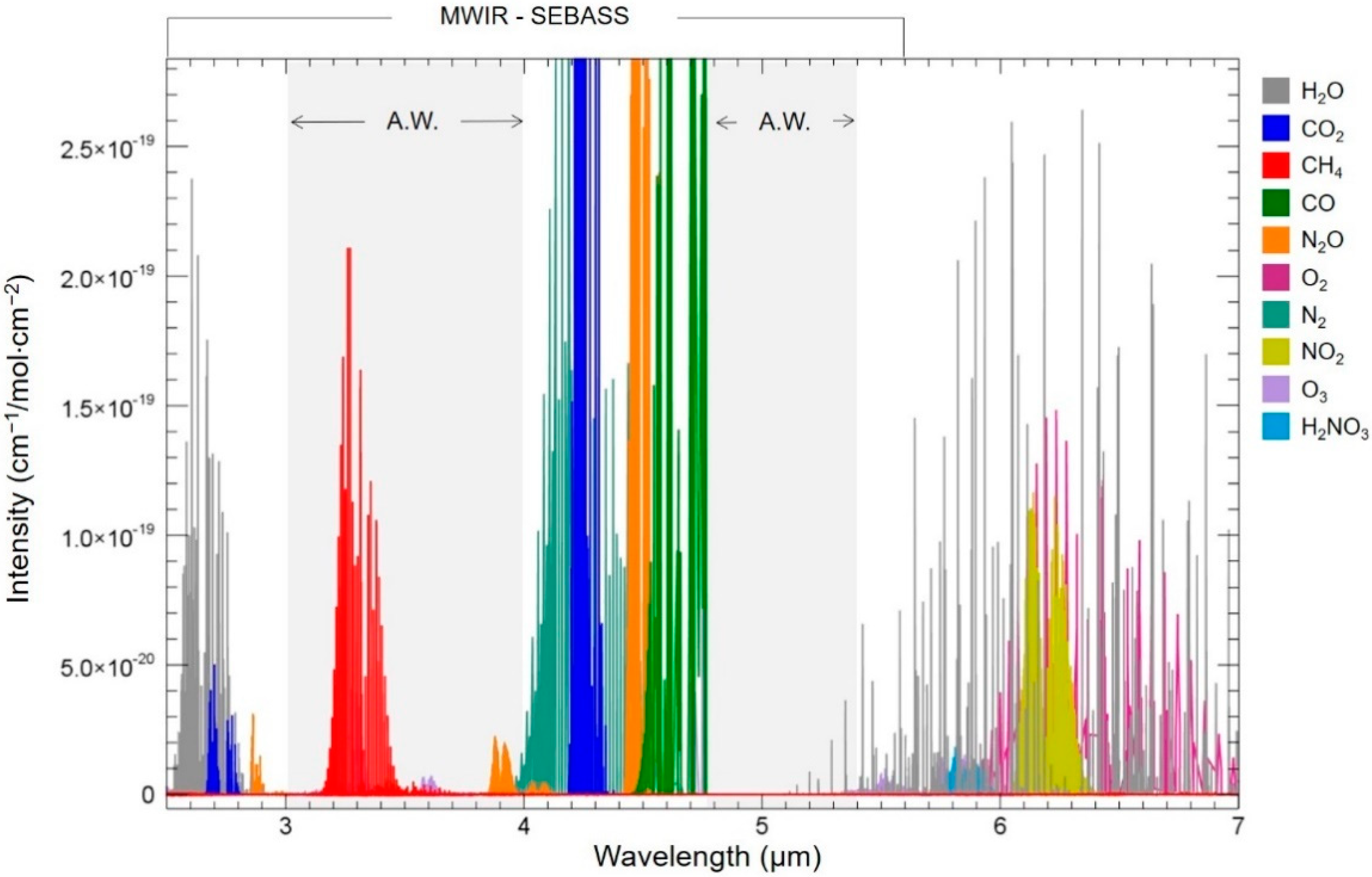
Here, we adopt the radiation model proposed by Griffin, et al. [11]. According to the authors, the MWIR is dominated by absorption bands of atmospheric gases (Figure 1). Since this interval incorporates both surface reflectance and emissivity from targets in general, the correction of the data acquired in the MWIR requires two steps: (i) compensation for atmospheric effects, aiming to estimate the radiance from the surface, and (ii) separation between temperature and emissivity from the compensated data [11].
The radiation model proposed by Griffin, et al. [11] (Equation (1)), assumes a plane-parallel atmosphere to calculate the total radiation that reaches the sensor (TOA):
where is expressed in W/m2-sr-µm, and:
- = Total radiance received at the sensor
- = Surface leaving radiance
- = Upwelling emitted atmospheric path radiance
- = Downwelling emitted atmospheric irradiance
- = Scattered path radiance at the sensor
- = Total (diffuse and direct) solar radiance that reaches the surface
- = Atmospheric transmittance—surface-sensor path
- = Surface emissivity
- = Blackbody radiance (Planck’s Function)
- = Surface temperature (K)
According to Griffin, et al. [11], path reflected solar radiance () and surface reflected downwelling thermal radiance ( provide around only 1–4% of the TOA at the atmospheric windows in the MWIR. Assuming that these components are neglectable, three terms remain to be calculated in Equation (2): path thermal (5–18%), surface emitted (: 56–65%) and reflected downwelling solar irradiance (: 22–30%), whose respective contributions are indicated in the parentheses.
- = Total radiance received at the sensor
- = Surface leaving radiance
- = Upwelling emitted atmospheric path radiance
- = Total (diffuse and direct) solar radiance that reaches the surface
- = Atmospheric transmittance—surface-sensor path
- = Surface emissivity
- = Blackbody radiance (Planck’s Function)
- = Surface temperature (K)
In Equation (2), solar reflected ( and surface leaving radiance () are dependent of the . To overcome this problem, Griffin, et al. [11] assume a constant value to , which leads to Equation (3) for the estimation of surface radiance (). According to the authors, the error associated to this assumption would be in the order of only 2–5% in the total radiance estimated at the 3–4 µm window of the MWIR:
where:
- = Surface leaving radiance
- = Upwelling radiance at the sensor for thermally emitted and absorbed radiation
- = Upwelling emitted atmospheric path radiance
- = Total (diffuse and direct) solar radiance that reaches the surface
- = Atmospheric transmittance—surface-sensor path
- = Surface emissivity
- = Blackbody radiance (Planck’s Function)
- = Surface temperature (K)
Plank’s Law establishes that the values of emissivity and temperature are wavelength () dependent. This condition implies that the errors associated to the estimated temperature values increase toward higher wavelengths, that is, the relation T/ε is less susceptible to errors in the MWIR range than in the LWIR [15].
3. Materials and Methods
3.1. Field Experiment
In August 2010 a controlled field experiment was performed at the former Rocky Mountain Oilfield Testing Center (RMOTC), located north of Casper, Wyoming (EUA) [2,16]. The experiment aimed to simulate possible scenarios of seepage and leakage of CH4, from natural and anthropogenic sources (i.e., pipelines and refineries). Controlled flow rates of gas were released from ground stations allocated at the surface (simulating anthropogenic sources) and subsurface (simulating natural sources). The gas flow fluctuated from 0.6 m3/h to 40 m3/h, as described in Table 1.
SEBASS flew over the experimental site on 20 August 2010, acquiring data on MWIR (2.5–5.2 µm) and LWIR (7.5–13.5 µm) wavelengths, simultaneously. Both sensors have a 1.1 mrad instantaneous field of view (IFOV), operating with 128 bands (128 cross-track pixels) and spectral resolutions of 0.025 µm in the MWIR, and 0.050 µm in the LWIR. The data were acquired at approximately 457 (1500 ft) and 762 (2500 ft) meters of altitude with spatial resolutions of 0.5 m and 0.84 m, respectively.
3.2. Atmospheric Correction and Data Calibration
MWIR data were processed using ENVI 5.3 software (Harris Geospatial Solutions Inc., Broomfield, CO, USA), assuming the model proposed by Griffin, et al. [11] for atmospheric compensation and emissivity retrieval. The same methodology was applied in the processing of the LWIR data.
Firstly, atmospheric effects were removed from the images using an adaptation of the in-scene atmospheric compensation (ISAC) algorithm [17,18]. The main advantage of this method relies on the fact that the algorithm only needs the data from the imagery to perform the atmospheric compensation. A uniform atmosphere and the presence of a surface similar to a black body in the scene (i.e., pixels with surface emissivity values close to 1) are assumed in the correction. Transmissivity () and upwelling radiance (), calculated with Equation (4) (Young, et al. [18] are used to define the atmospheric compensation spectrum:
These values are calculated based on the brightness temperature of each pixel. After evaluating each pixel in the scene, the algorithm selects the spectral channel with the highest number of pixels with maximum values of brightness temperature (i.e., pixels with as a reference channel. A scatter plot of and is build for this channel and a linear fit is made through a regression line adjusted to the upper top of the plot (i.e., values closer to ). and values are then estimated from the slope and intercession point in respectively, for each channel, and used to estimate the surface radiance of each pixel, without the atmospheric interference.
Emissivity was estimated using the emissivity normalization algorithm [19,20,21]. The algorithm estimates the temperature for each pixel using the radiance values calculated in the previous step and assuming a fixed value of maximum emissivity for all pixels in every of the image. The maximum temperature estimated for each pixel is then selected as the brightness temperature of the surface, which is subsequently used to calculate the emissivity in the scene through Equation (5):
where:
- = emissivity for pixel
- = radiance measured in for pixel
- = upward radiance
- = atmospheric transmissivity for
- = downward radiance
- = Blackbody radiance (Planck’s Function)
- = highest temperature of the calculated temperatures for pixel
3.3. Detection of Methane Plumes
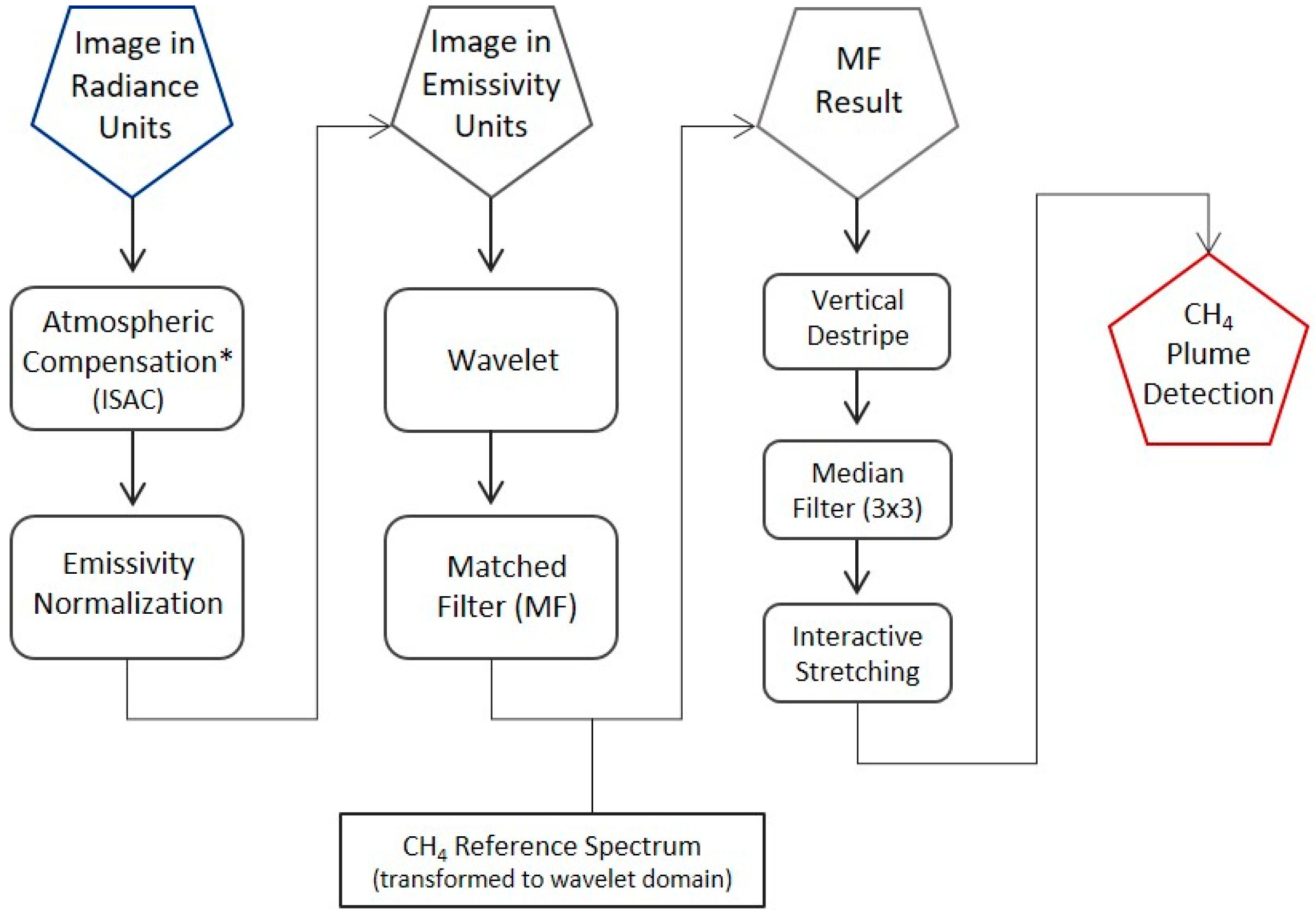
The methodology applied for CH4 plume detection is presented in Figure 2. The images in emissivity units were processed using a wavelet transform for simultaneous de-noising and spectral enhancement. The matched filter (MF) algorithm [22] was used for the isolation of the plume in the scene. A reference spectral signature of the CH4 acquired from National Institute of Standards and Technology (NIST) [23] database, resampled for SEBASS spectral resolution and transformed with the wavelet code, was used as an endmember for imaging classification with the MF. In addition, a median filter (3 × 3) was applied to the resulting image. This methodology was applied in the processing of MWIR and LWIR images. Each step is detailed in the next sections.
3.3.1. Wavelets
The wavelet transform comprises a processing tool that decomposes the original signal (i.e., image) in time and frequency domains, thus representing the image in multi-scales [24,25,26]. Once the wavelet components are computed, the noise is concentrated at the lowest scales while the continuum remains at the highest scales. By eliminating the top and bottom components and summing the remaining scales a high quality product is generated. This product is obtained by (i) filtering the noise in the image; (ii) highlighting spectral features; (iii) decreasing the spectral continuum variability introduced from variations in illumination and topography; and (iv) minimization of residuals from atmospheric correction and temperature estimation [27,28]. Another advantage of the method comprises the comparison between data acquired at different wavelengths. Since the spectra is normalized to zero mean, the data acquired at different wavelengths will have the same weight and scale after the wavelet transform, allowing both to be comparable. The wavelet function used to decomposed the image into nine (9) components consists of the second derivative of a Gaussian function (e.g., DOG [29]). The final image is the result of the sum of components 3, 4, 5, and 6. The remaining components are discarded.
3.3.2. Matched Filter
A matched filter (MF) is a classification algorithm used for the detection of known targets in the scene through the estimate of the abundance of an endmember at the sub-pixel scale [30,31]. The suppression of the background components maximizes the signal of the endmembers, enhancing the signature of the target. The final result consists of a grayscale image with minimum variance, divided into MF scores varying between 0–1. MF scores represent the fraction of the pixels that contains the endmember’s spectral signature. Values close to 0 are attributed to pixels from the background, and values close to 1 to pixels from the target [32]. To isolate the target from the background, a limit value “X” of the MF score is defined by the user. Adjusting the histogram at this limit, only pixels with MF scores between “X − 1” are going to be highlighted in the scene. Here, we defined a minimum MF score (X) of 0.7 for the detection of the plume.
The main advantage of the method relies on target detection based on a reference spectrum (e.g., extracted from the image, acquired in the field or available on spectral libraries), eliminating the need to acquire data from the remaining elements comprising the scene background. The drawback of the MF is the possibility of false positives if other materials with C–H in the composition (e.g., HC based plastic, paint, alphalt) or rare materials not related to the target occur in the image [33].
4. Results
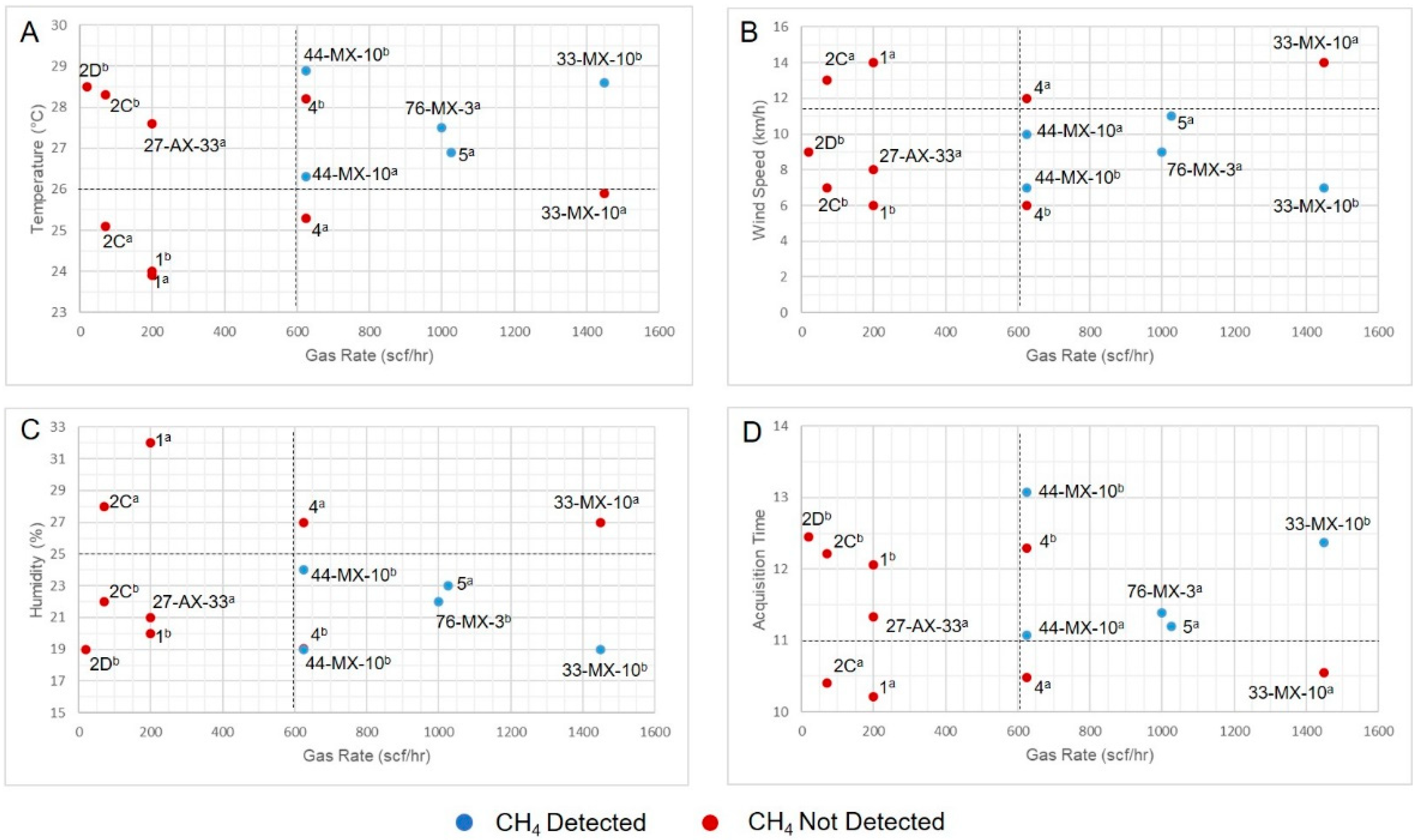
Results obtained from processing SEBASS data show that the CH4 plume was identified distinctly in the MWIR and LWIR ranges (Table 2). Figure 3 shows plots of gas rate versus the acquisition time and weather condition (temperature, humidity, wind speed) data, acquired simultaneously to SEBASS airborne survey for each gas station. The minimum and maximum flow rate detected in both ranges were 18 m3/h and 40 m3/h, respectively. Pixels containing CH4 spectral features (i.e., centered at 3.3 µm and 7.9 µm) were mapped in both datasets, exhibiting simultaneity in plume position and spatial distribution. The plumes were identified in all stations in the LWIR images [2]. However, in the MWIR data, the gas was detected only at four out of the nine ground stations: 44-MX-10 (18 m3/h), 76-MX-3 (28 m3/h), 5 (29 m3/h), and 33-MX-10 (40 m3/h). Here, only the results with positive plume detection in both intervals are presented (Figure 4, Figure 5 and Figure 6).
Spectra extracted from pixels of the gas plumes from stations with highest flow rates (i.e., 5 and 33-MX-10) are shown in Figure 7. In both sets of signatures, the CH4 features centered at 3.3 µm (MWIR) and 7.7–7.8 µm (LWIR) stand out. In the spectral collection extracted from the LWIR images, a decrease in the feature depth as the pixels move forward from the emission source is noted, as firstly described by Scafutto, et al. [2]. However, in the images acquired in the MWIR range, this relation is only observed in the spectral collection extracted from Station 5.
The wavelet transform reduced the noise (Figure 8), improving the quality of the image. With the application of wavelet and MF, the CH4 plume was isolated from the background. The number of pixels identified in each station retains proportionality with the flow rates of the experiment (Table 2). Additionally, the plume direction agrees with the main wind direction (Table 2—data collected concomitantly with the airborne surveys).
5. Discussion
Assuming the radiative transfer model proposed by Griffin, et al. [11], the images acquired at MWIR and LWIR ranges with the SEBASS sensor over the field experiment of controlled CH4 release were processed using the same methodology for atmospheric compensation, emissivity retrieval, and plume mapping. The results obtained from the airborne data collected in this range proved inferior when compared to those yielded in the LWIR window, since the radiation emitted by CH4 in ambient conditions is very low in the MWIR range (see Figure S2 in Supplementary Materials).
The processing of MWIR data using methodologies usually applied to LWIR images led to the detection of the CH4 plumes. However, due to the lower strength of the 3.3 μm feature under ambient conditions and the greater amount of noise in the MWIR images, the use of more sophisticated enhanced techniques is necessary to isolate the target from the background.
Considering the emissivity spectra extracted from the pixels from each plume (Figure 8), it is noted that the values for the CH4 feature in the LWIR are close to 1 (~0.92). Nevertheless, the emissivity retrieved for the same pixels are considerably smaller for the CH4 feature in the MWIR (~0.2). The relation between emissivity () and reflectance () postulated by Kirchhoff’s Law [34] establishes that the sum of the components must be equal to 1, which results in for the CH4 feature in the LWIR and in the MWIR feature. Reflectance overcomes emissivity values in the MWIR range. This corresponds to ten times the value of the reflectance in the LWIR. Therefore, the influence of reflectance must be considered in the radiative transference model to achieve better results, as proposed by Griffin, et al. [11] and Mushkin, et al. [12].
Apart from flow rate and background temperature, humidity, wind speed and time of data acquisition also influence in the detection of CH4 plumes (Figure 3). Based on the conditions prevailing during the experiment, results demonstrate that there is a threshold for proper plume sensing using MWIR wavelengths. In the Casper experiment, best results were yielded from data collected after 11:00 a.m., at temperatures greater than 25 °C, at humidity levels lower than 25% and at wind speeds inferior to 10 km/h. The hour of the day is related to the solar incidence angle. Between 11:00 a.m. and 13:00 p.m. the Sun is at its maximum, and so is the incidence angle, diminishing the scattering of solar radiation. The increase of the atmospheric temperature will also warm up the plume, enhancing the contrast against the background. The lower the humidity, the lower the interference of atmospheric components (especially H2O), favoring plume detection.
The only exception occurs with the ground station 4b (Figure 3). Despite the fact that the image over this station was acquired under favorable parameters for CH4 detection, it seems that the low wind speed (i.e., 6 km/h) was insufficient to disperse the plume at the time of the survey. Therefore, the pixels of the plume were concentrated in a few pixels in the image, preventing the detection of an actual plume.
Along-wind (AW) and cross-wind (CW) profiles extracted from LWIR and MWIR images are illustrated in Figure 9. They show that the values of emissivity for background pixels are more homogeneous in the LWIR. The difference between the maximum and minimum values of emissivity for background pixels are 0.02 CW and 0.03 AW in the LWIR plots. This difference is larger for the MWIR images, i.e., 0.4 CW and 0.5 AW. The higher variability of emissivity values of the pixels around the average background hampers the isolation of the plume in the MWIR.
The application of the wavelet transform was essential to overcome these problems. The use of this technique enhanced the signal of the gas, since the background values of the pixels in the wavelet image are less variable in comparison to emissivity images. Furthermore, as shown in the spectral signatures in Figure 8, it is noticed that once the wavelet normalizes the spectrum, the background is concentrated around zero, enhancing the CH4 feature in both wavelengths. However, in the MWIR range, the width of the spectral feature of the plume is enlarged. This is due to the fact that the lower wavelet scales were discarded in the overall feature enhancing process, and so the feature originally located between 3.1 and 3.5 µm incorporated part of the wavelengths corresponding to background pixels (feature spanning between 3.0 and 4 µm in the wavelet domain), which may lead to the detection of false positives.
Another advantage of the wavelets comprises the significant decrease of the noise in the image [35], which also has positive consequences on the CH4 spectral signatures (Figure 8). Compared to the signatures presented by Scafutto, et al. [2] in their previous work with raw LWIR emissivity data, here the wavelet version of the CH4 feature at 7.7 µm, as well as its variation due to the distance from the emission source, are much better defined (Figure 8). The same is observed in the MWIR spectra.
6. Conclusions
Considering a controlled field experiment, here we show, for the first time, the detection of CH4 plumes using airborne MWIR hyperspectral data. The high resolution and low signal to noise ratio of the SEBASS sensor enabled the detection of the plumes using methods usually applied to LWIR images, when combined with wavelet transform. It was demonstrated that, despite the interference of the reflectance in this range, it was possible to detect the CH4 plume in the atmospheric window between 3–4 µm. Flow rates equal or higher than 18 m3/h (four out of nine gas stations) were detected in images acquired at 457 m and 762 m altitude. The analysis of the spectral signature extracted from the plumes evidenced that the application of the wavelet transform was essential for the detection of the gas; reducing the noise in the image and enlarging the contrast between plume and background pixels and, thus, highlighting the CH4 feature. Additionally, we demonstrated that the acquisition time and weather conditions, such as temperature, humidity, and wind speed, hamper detection, and so limits of each of these variables must be considered for successful approaches on CH4 plume detection using daytime MWIR data.
Supplementary Materials
The following are available online at https://0-www-mdpi-com.brum.beds.ac.uk/2072-4292/10/8/1237/s1, Figure S1. HITRAN spectral lines of methane (CH4) at the temperature of 296 K [18]. Location of fundamental vibrations is indicated in the plot as v1, v2, v3, v4; Figure S2. Methane self-emission spectrum acquired under ambient conditions (298 K/25 °C) with the HYPER-CAM MWE (1.5–5 µm) and the HYPER-CAM METHANE (7.4–8.3 µm) hyperspectral cameras operated by TELOPS INC. (Quebec City, QC, Canada—http://telops.com/products/hyperspectral-cameras). Both cameras have user-selectable spectral resolution up to 0.25 cm−1 and a NESR* (nw/cm2 s cm−1) of 7 and 6 for MWIR and LWIR respectively (* noise equivalent spectral radiance).
Author Contributions
Conceptualization, C.R.d.S.F. and R.D.P.M.S; Methodology, R.D.P.M.S and C.R.d.S.F.; Formal Analysis, R.D.P.M.S and C.R.d.S.F.; Investigation, R.D.P.M.S and C.R.d.S.F; Resources, C.R.d.S.F.; Writing—Original Draft Preparation, R.D.P.M.S and C.R.d.S.F; Writing—Review & Editing, R.D.P.M.S and C.R.d.S.F; Visualization, R.D.P.M.S and C.R.d.S.F; Supervision, C.R.d.S.F; Project Administration, C.R.d.S.F.; Funding Acquisition, C.R.d.S.F. and R.D.P.M.S.
Funding
This research was funded by Petrobras (Rio de Janeiro, RJ, Brazil) under the project “Hyperspectral and Hyperthermal Hydrocarbon Detection”, FAPESP (São Paulo, SP, Brazil) (research grant. no. 2015/19842-7) and CNPq (Brasília, DF, Brazil) (research grant no. 2008-7/303563).
Acknowledgments
The authors would like to thank Wilson Jose de Oliveira and Dean N. Riley for the assistance in the conception, execution and database creation of the project, and Petrobras for funding the experiment. We are indebted to the U.S. DOE and RMOTC staff for support and assistance in the field and FotoTerra (São Paulo, SP, Brazil), Spectir (Reno, NV, USA), and The Aerospace Corporation (El Segundo, CA, USA) for airborne campaigns over the experimental site. We are grateful to Neil Pendok for the assistance in the development of the wavelet code. R.D.P.M.S. and C.R.d.S.F. also acknowledge FAPESP (research grant. bo. 2015/19842-7) and CNPq (research grant no. 2008-7/303563) for financial support.
Conflicts of Interest
The authors declare no conflict of interest.
References
- Hulley, G.C.; Duren, R.M.; Hopkins, F.M.; Hook, S.J.; Johnson, W.R.; Eng, B.T.; Mihaly, J.M.; Jovanovic, V.M.; Chazanoff, S.L.; Staniszewski, Z.K. High spatial resolution imaging of methane and other trace gases with the airborne Hyperspectral Thermal Emission Spectrometer (HyTES). Atmos. Meas. Tech. 2016, 9, 2393. [Google Scholar] [CrossRef]
- Scafutto, R.D.M.; de Souza Filho, C.R.; Riley, D.N.; de Oliveira, W.J. Evaluation of thermal infrared hyperspectral imagery for the detection of onshore methane plumes: Significance for hydrocarbon exploration and monitoring. Int. J. Appl. Earth Observ. Geoinf. 2018, 64, 311–325. [Google Scholar] [CrossRef]
- Thorpe, A.; Frankenberg, C.; Roberts, D. Retrieval techniques for airborne imaging of methane concentrations using high spatial and moderate spectral resolution: Application to AVIRIS. Atmos. Meas. Tech. 2014, 7, 491–506. [Google Scholar] [CrossRef]
- Nielsen, A.H.; Nielsen, H.H. The infrared absorption bands of methane. Phys. Rev. 1935, 48, 864. [Google Scholar] [CrossRef]
- Bradley, E.S.; Leifer, I.; Roberts, D.A.; Dennison, P.E.; Washburn, L. Detection of marine methane emissions with AVIRIS band ratios. Geophys. Res. Lett. 2011, 38. [Google Scholar] [CrossRef] [Green Version]
- Kastek, M.; Piątkowski, T.; Dulski, R.; Chamberland, M.; Lagueux, P.; Farley, V. Method of gas detection applied to infrared hyperspectral sensor. Photonics Lett. Pol. 2012, 4, 146–148. [Google Scholar] [CrossRef]
- Roberts, D.A.; Bradley, E.S.; Cheung, R.; Leifer, I.; Dennison, P.E.; Margolis, J.S. Mapping methane emissions from a marine geological seep source using imaging spectrometry. Remote Sens. Environ. 2010, 114, 592–606. [Google Scholar] [CrossRef]
- Thorpe, A.K.; Roberts, D.A.; Bradley, E.S.; Funk, C.C.; Dennison, P.E.; Leifer, I. High resolution mapping of methane emissions from marine and terrestrial sources using a Cluster-Tuned Matched Filter technique and imaging spectrometry. Remote Sens. Environ. 2013, 134, 305–318. [Google Scholar] [CrossRef]
- Tratt, D.M.; Buckland, K.N.; Hall, J.L.; Johnson, P.D.; Keim, E.R.; Leifer, I.; Westberg, K.; Young, S.J. Airborne visualization and quantification of discrete methane sources in the environment. Remote Sens. Environ. 2014, 154, 74–88. [Google Scholar] [CrossRef]
- Hall, J.L.; Boucher, R.H.; Buckland, K.N.; Gutierrez, D.J.; Hackwell, J.A.; Johnson, B.R.; Keim, E.R.; Moreno, N.M.; Ramsey, M.S.; Sivjee, M.G. MAGI: A New High-Performance Airborne Thermal-Infrared Imaging Spectrometer for Earth Science Applications. IEEE Trans. Geosci. Remote Sens. 2015, 53, 5447–5457. [Google Scholar] [CrossRef]
- Griffin, M.K.; Burke, H.-H.K.; Kerekes, J.P. Understanding radiative transfer in the midwave infrared: A precursor to full-spectrum atmospheric compensation. In Proceedings of the Algorithms and Technologies for Multispectral, Hyperspectral, and Ultraspectral Imagery X, Orlando, FL, USA, 12–15 April 2004; Volume 5425, pp. 348–357. [Google Scholar]
- Mushkin, A.; Balick, L.K.; Gillespie, A.R. Extending surface temperature and emissivity retrieval to the mid-infrared (3–5 μm) using the Multispectral Thermal Imager (MTI). Remote Sens. Environ. 2005, 98, 141–151. [Google Scholar] [CrossRef]
- Hackwell, J.A.; Warren, D.W.; Bongiovi, R.P.; Hansel, S.J.; Hayhurst, T.L.; Mabry, D.J.; Sivjee, M.G.; Skinner, J.W. LWIR/MWIR imaging hyperspectral sensor for airborne and ground-based remote sensing. In Proceedings of the SPIE’s 1996 International Symposium on Optical Science, Engineering, and Instrumentation, Denver, CO, USA, 4–9 August 1996; pp. 102–107. [Google Scholar]
- Gordon, I.E.; Rothman, L.S.; Hill, C.; Kochanov, R.V.; Tan, Y.; Bernath, P.F.; Birk, M.; Boudon, V.; Campargue, A.; Chance, K. The HITRAN2016 molecular spectroscopic database. J. Quant. Spectrosc. Radiat. Transf. 2017, 203, 3–69. [Google Scholar] [CrossRef]
- Salisbury, J.W.; D’Aria, D.M. Emissivity of terrestrial materials in the 3–5 μm atmospheric window. Remote Sens. Environ. 1994, 47, 345–361. [Google Scholar] [CrossRef]
- Scafutto, R.D.P.M.; de Souza Filho, C.R.; de Oliveira, W.J. Hyperspectral remote sensing detection of petroleum hydrocarbons in mixtures with mineral substrates: Implications for onshore exploration and monitoring. ISPRS J. Photogramm. Remote Sens. 2017, 128, 146–157. [Google Scholar] [CrossRef]
- Kirkland, L.; Herr, K.; Keim, E.; Adams, P.; Salisbury, J.; Hackwell, J.; Treiman, A. First use of an airborne thermal infrared hyperspectral scanner for compositional mapping. Remote Sens. Environ. 2002, 80, 447–459. [Google Scholar] [CrossRef] [Green Version]
- Young, S.J.; Johnson, B.R.; Hackwell, J.A. An in-scene method for atmospheric compensation of thermal hyperspectral data. J. Geophys. Res. Atmos. 2002, 107. [Google Scholar] [CrossRef] [Green Version]
- Gillespie, A.R.; Matsunaga, T.; Rokugawa, S.; Hook, S.J. Temperature and emissivity separation from advanced spaceborne thermal emission and reflection radiometer (ASTER) images. In Proceedings of the SPIE’s 1996 International Symposium on Optical Science, Engineering, and Instrumentation, Denver, CO, USA, 4–9 August 1996; pp. 82–95. [Google Scholar]
- Hook, S.J.; Gabell, A.R.; Green, A.A.; Kealy, P.S. A comparison of techniques for extracting emissivity information from thermal infrared data for geologic studies. Remote Sens. Environ. 1992, 42, 123–135. [Google Scholar] [CrossRef]
- Li, Z.-L.; Becker, F.; Stoll, M.; Wan, Z. Evaluation of six methods for extracting relative emissivity spectra from thermal infrared images. Remote Sens. Environ. 1999, 69, 197–214. [Google Scholar] [CrossRef]
- Boardman, J.W.; Kruse, F.A.; Green, R.O. Mapping target signatures via partial unmixing of AVIRIS data. In Summaries of: Fifth JPL Airborne Earth Science Workshop; JPL Publication: Pasadena, CA, USA, 1995; Volume 1, pp. 23–26. [Google Scholar]
- Linstrom, P.J.; Mallard, W.G. The NIST Chemistry WebBook: A chemical data resource on the internet. J. Chem. Eng. Data 2001, 46, 1059–1063. [Google Scholar] [CrossRef]
- Walczak, B.; Bouveresse, E.; Massart, D. Standardization of near-infrared spectra in the wavelet domain. Chemom. Intell. Lab. Syst. 1997, 36, 41–51. [Google Scholar] [CrossRef]
- Xu, Y.; Weaver, J.B.; Healy, D.M.; Lu, J. Wavelet transform domain filters: A spatially selective noise filtration technique. IEEE Trans. Image Process. 1994, 3, 747–758. [Google Scholar] [PubMed]
- Zhang, X.; Younan, N.H.; O’Hara, C.G. Wavelet domain statistical hyperspectral soil texture classification. IEEE Trans. Geosci. Remote Sens. 2005, 43, 615–618. [Google Scholar] [CrossRef]
- Feng, J.; Rogge, D.; Rivard, B. Comparison of lithological mapping results from airborne hyperspectral VNIR-SWIR, LWIR and combined data. Int. J. Appl. Earth Observ. Geoinf. 2018, 64, 340–353. [Google Scholar] [CrossRef]
- Weaver, J.B.; Xu, Y.; Healy, D.; Cromwell, L. Filtering noise from images with wavelet transforms. Magn. Reson. Med. 1991, 21, 288–295. [Google Scholar] [CrossRef] [PubMed]
- Muraki, S. Multiscale volume representation by a DoG wavelet. IEEE Trans. Vis. Comput. Graph. 1995, 1, 109–116. [Google Scholar] [CrossRef]
- Boardman, J.W.; Kruse, F.A. Analysis of Imaging Spectrometer Data Using N-Dimensional Geometry and a Mixture-Tuned Matched Filtering Approach. IEEE Trans. Geosci. Remote Sens. 2011, 49, 4138–4152. [Google Scholar] [CrossRef]
- Harsanyi, J.C.; Chang, C.-I. Hyperspectral image classification and dimensionality reduction: An orthogonal subspace projection approach. IEEE Trans. Geosci. Remote Sens. 1994, 32, 779–785. [Google Scholar] [CrossRef]
- Manolakis, D.; Marden, D.; Shaw, G.A. Hyperspectral image processing for automatic target detection applications. Linc. Lab. J. 2003, 14, 79–116. [Google Scholar]
- Manolakis, D.; Truslow, E.; Pieper, M.; Cooley, T.; Brueggeman, M. Detection algorithms in hyperspectral imaging systems: An overview of practical algorithms. IEEE Signal Process. Mag. 2014, 31, 24–33. [Google Scholar] [CrossRef]
- Rees, W.G. Physical Principles of Remote Sensing; Cambridge University Press: Cambridge, UK, 2012; p. 247. [Google Scholar]
- Scafutto, R.D.P.M.; Souza Filho, C.R.d.; Rivard, B. Characterization of mineral substrates impregnated with crude oils using proximal infrared hyperspectral imaging. Remote Sens. Environ. 2016, 179, 116–130. [Google Scholar] [CrossRef]
Figure 1.
HITRAN spectral lines (extracted from [14]) for primary absorbing gases in the atmosphere in the MWIR range (3–5 µm). Areas in grey outline the atmospheric windows between 3–4 µm and 4.6–5.3 µm. The region covered by the MWIR SEBASS sensor (2.4–5.5 µm) is indicated in the upper part of the plot. A.W.: atmospheric window.

Figure 2.
Diagram of the methodology applied for the detection of CH4 plumes. * Adaptation of the in-scene atmospheric compensation algorithm [18].
Figure 2.
Diagram of the methodology applied for the detection of CH4 plumes. * Adaptation of the in-scene atmospheric compensation algorithm [18].

Figure 3.
Metrics of ambient conditions—(A) temperature, (B) wind speed, (C) humidity, (D) acquisition time—versus gas rate during the SEBASS airborne survey for each gas station (named on the plots). Superscript letters after gas station names correspond to acquisition altitudes at (a) = 457 m and (b) 762 m. Dashed lines limit the quadrants where temperature, wind speed, humidity, and acquisition time favored the detection of CH4 plumes in the experiment.

Figure 4.
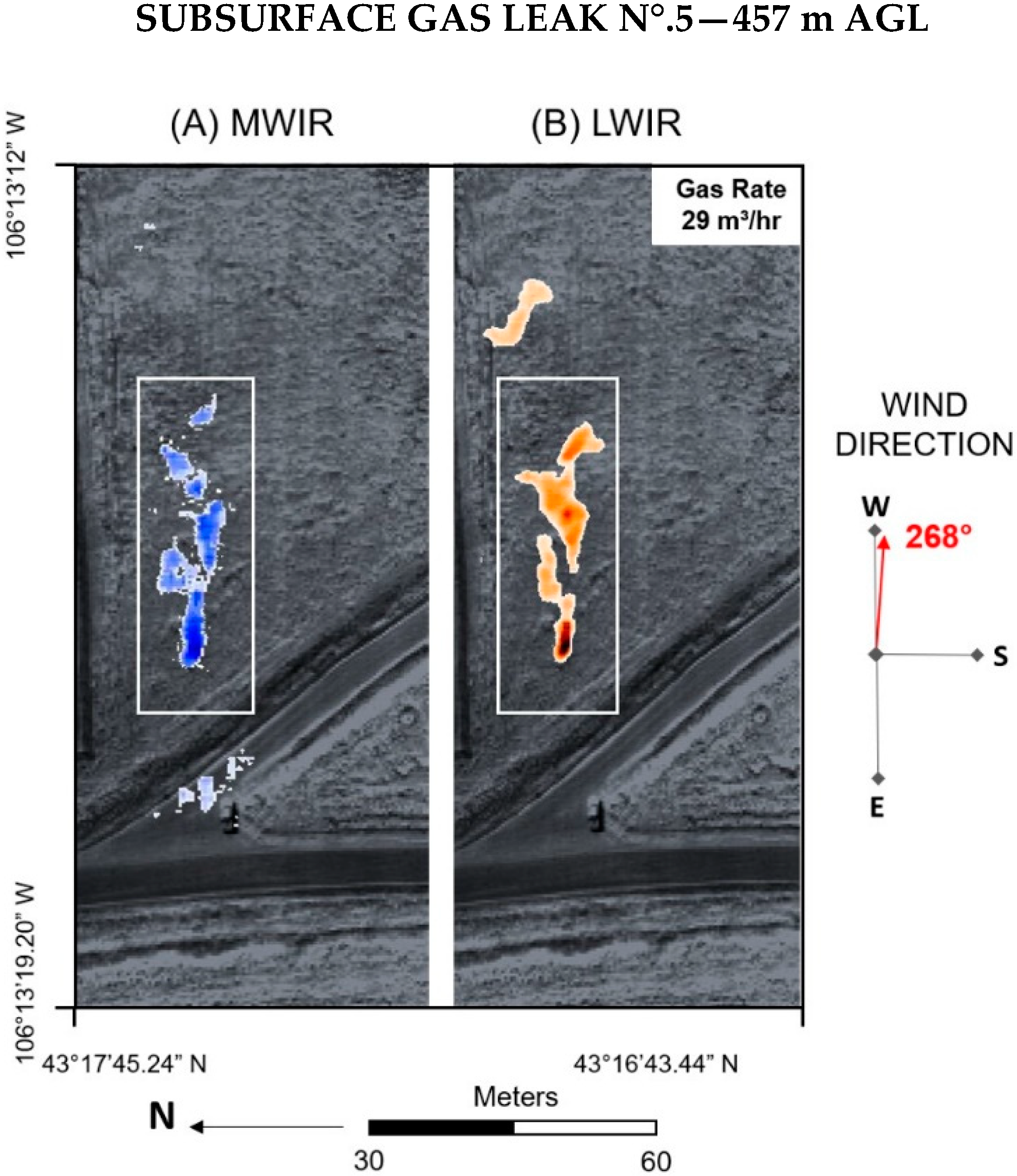
Detection of CH4 plumes in the (A) MWIR and (B) LWIR ranges—SEBASS flight performed on 20 August 2010 over station 5 (gas source: RMOTC—injection) at 11:20:26 (local time) with 0.50 m spatial resolution and at 457 m AGL. The red square indicates the ground station location (i.e., source of gas leak) and the respective plume. Pixels in blue (A) and red (B) indicate the occurrence of methane in the scenes. The main direction of the wind is displayed in the diagram on the right side of the figure (data collected between 11:00 p.m.–12:00 p.m.).
Figure 4.
Detection of CH4 plumes in the (A) MWIR and (B) LWIR ranges—SEBASS flight performed on 20 August 2010 over station 5 (gas source: RMOTC—injection) at 11:20:26 (local time) with 0.50 m spatial resolution and at 457 m AGL. The red square indicates the ground station location (i.e., source of gas leak) and the respective plume. Pixels in blue (A) and red (B) indicate the occurrence of methane in the scenes. The main direction of the wind is displayed in the diagram on the right side of the figure (data collected between 11:00 p.m.–12:00 p.m.).

Figure 5.
Detection of CH4 plumes in the (A) MWIR and (B) LWIR ranges—SEBASS flight performed on 20 August 2010 over station 76-MX-3 (gas source: RMOTC) at 11:39:17 (local time) with 0.50 m spatial resolution and at 457 m above ground level (AGL). The red square indicates the ground station location (i.e., source of gas leak) and the respective plume. Pixels in blue (A) and red (B) indicate the occurrence of methane in the scenes. The main direction of the wind is displayed in the diagram on the right side of the figure (data collected between 11:30 p.m.–12:30 p.m.).

Figure 6.
Detection of CH4 plumes in the (A) MWIR and (B) LWIR ranges—SEBASS flight performed on 20 August 2010 over station 44-MX-10 (gas source: RMOTC—injection) at (1) 11:07:59 (local time) with 0.50 m spatial resolution and at 457 m AGL and (2) 13:08:18 (local time) with 0.84 m spatial resolution and at 762 m AGL. The red square indicates the ground station location (i.e., source of the gas leak) and respective plume. Pixels in blue (A) and red (B) indicate the occurrence of methane in the scene. The main direction of the wind is displayed in the diagram on the right side of the figure (data collected between (1) 10:30 p.m.–11:30 p.m. and (2) 12:30 p.m.–13:30 p.m.).

Figure 7.
SEBASS MWIR (A,C) and LWIR (B,D) spectral signatures in the wavelet domain extracted from pixels near and far from emission sources. (A,B) Station 5 (subsurface leak of 29 m3/h; data acquisition at 457 m). (C,D) Station 33-MX-10 (surface leak of 41.1 m3/h; data acquisition at 762 m). Main absorption features are indicated in each plot.

Figure 8.
Comparison between spectral signatures extracted from the same pixels. (A,C): images in emissivity units. (B,D): images transformed to the wavelet domain. The spectra were extracted from the CH4 plume formed from Leak 5 from MWIR (A,B) and LWIR (C,D) images. Areas in grey outline the CH4 features centered at 3.3 µm and 7.7 µm in the respective plots. Spectra were interrupted within regions highly affected by atmospheric interference. The wavelet decreased the noise and increased the contrast between the plume and the background (indicated by the black arrows in the plots). The same improvements were noticed in the spectral collection extracted in other leakage stations.

Figure 9.
Along-wind (AWP) and cross-wind (CW) profiles of MWIR (A) and LWIR (B) images acquired over Station 5. Areas in grey outline the CH4 features centered at 3.3 µm and 7.7 µm in the respective plots. The difference between emissivity values of the pixels of the plume (P) and background (B) is expressive in the LWIR images whereas, for the MWIR, this difference is impaired due to the proximity of the average values between the plume and background.


Table 1.
Specifications of CH4 leak stations and data acquisition parameters, including: emission rates from each station (m3/h and SCFH), acquisition altitude (m), acquisition time and meteorological data acquired at RMOTC with a weather station during the experiment. Weather data was collected on 20 August 2010 every five minutes, from 8:00 a.m. to 2:00 p.m. Temperature, humidity, and wind speed and direction presented in this table corresponds to data collected concomitantly with the time of the airborne survey over each gas leakage station.
| Acquisition Conditions | |||||||||
|---|---|---|---|---|---|---|---|---|---|
| Station | Configuration | Gas Source | Gas Rate (m3/h/SCFH) | Altitude (m) | Time (Local) | Temperature (°C) | Humidity (%) | Wind Speed (km/h) | Wind Direction |
| 1 | Subsurface | RMOTC (injection) | 6.0/200 | 457 | 10:22:07 | 23.9 | 32 | 14 | SSW |
| 2C | Subsurface | Cylinder | 2.0/70 | 457 | 10:41:48 | 25.1 | 28 | 13 | SSW |
| 4 | Subsurface | RMOTC (injection) | 18.0/625 | 457 | 10:48:07 | 25.3 | 27 | 12 | SSW |
| 33-MX-10 | Surface | RMOTC (injection) | 40.0/1450 | 457 | 10:55:21 | 25.9 | 27 | 14 | SSW |
| 44-MX-10 | Surface | RMOTC (injection) | 18.0/625 | 457 | 11:07:59 | 26.3 | 24 | 10 | SSW |
| 5 | Subsurface | RMOTC (injection) | 29.0/1025 | 457 | 11:20:26 | 26.9 | 23 | 11 | SSW |
| 27-AX-33 | Surface | RMOTC (injection) | 6.0/200 | 457 | 11:33:01 | 27.6 | 21 | 8 | SW |
| 76-MX-3 | Surface | RMOTC | 28.0/1000 | 457 | 11:39:17 | 27.5 | 22 | 9 | SSW |
| 1 | Subsurface | RMOTC (injection) | 6.0/200 | 762 | 12:06:13 | 24.0 | 20 | 6 | SSW |
| 2C | Subsurface | Cylinder | 2.0/70 | 762 | 12:21:07 | 28.3 | 22 | 7 | SSW |
| 4 | Subsurface | RMOTC (injection) | 18.0/625 | 762 | 12:29:37 | 28.2 | 19 | 6 | SSW |
| 33-MX-10 | Surface | RMOTC (injection) | 40.0/1450 | 762 | 12:37:31 | 28.6 | 19 | 7 | WNW |
| 2D | Subsurface | Cylinder | 0.6/20 | 762 | 12:45:19 | 28.5 | 19 | 9 | W |
| 44-MX-10 | Surface | RMOTC (injection) | 18.0/625 | 762 | 13:08:17 | 28.9 | 19 | 7 | SSW |
Table 2.
Detection of CH4 plumes in the MWIR and LWIR ranges. Superscript letters indicate the image acquisition altitude at (a) 457 m and at (b) 762 m. ✓ = CH4 plume detected/x = CH4 plume not detected.
Table 2.
Detection of CH4 plumes in the MWIR and LWIR ranges. Superscript letters indicate the image acquisition altitude at (a) 457 m and at (b) 762 m. ✓ = CH4 plume detected/x = CH4 plume not detected.
| Detection | ||||
|---|---|---|---|---|
| Gas Station | Gas Rate (m3/h/SCFH) | WIND (Speed—Direction) | MWIR | LWIR |
| 2Db | 0.6/20 | 19 km/h—W | x | ✓ |
| 2Ca | 2.0/70 | 13 km/h—SSW | x | ✓ |
| 2Cb | 2.0/70 | 7 km/h—SSW | x | ✓ |
| 1a | 6.0/200 | 14 km/h—SSW | x | ✓ |
| 1b | 6.0/200 | 6 km/h—SSW | x | ✓ |
| 27-AX-33a | 6.0/200 | 8 km/h—SW | x | ✓ |
| 4a | 18.0/625 | 12 km/h—SSW | x | ✓ |
| 4b | 18.0/625 | 6 km/h—SSW | x | ✓ |
| 44-MX-10a | 18.0/625 | 10 km/h—SSW | ✓ | ✓ |
| 44-MX-1 b | 18.0/625 | 7 km/h—SSW | ✓ | ✓ |
| 76-MX-3a | 28.0/1000 | 9 km/h—SSW | ✓ | ✓ |
| 5a | 29.0/1025 | 11 km/h—SSW | ✓ | ✓ |
| 33-MX-10a | 40.0/1450 | 14 km/h—SSW | x | ✓ |
| 33-MX-10b | 40.0/1450 | 7 km/h—WNW | ✓ | ✓ |
© 2018 by the authors. Licensee MDPI, Basel, Switzerland. This article is an open access article distributed under the terms and conditions of the Creative Commons Attribution (CC BY) license (http://creativecommons.org/licenses/by/4.0/).
Share and Cite
MDPI and ACS Style
Scafutto, R.D.P.M.; De Souza Filho, C.R. Detection of Methane Plumes Using Airborne Midwave Infrared (3–5 µm) Hyperspectral Data. Remote Sens. 2018, 10, 1237. https://0-doi-org.brum.beds.ac.uk/10.3390/rs10081237
AMA Style
Scafutto RDPM, De Souza Filho CR. Detection of Methane Plumes Using Airborne Midwave Infrared (3–5 µm) Hyperspectral Data. Remote Sensing. 2018; 10(8):1237. https://0-doi-org.brum.beds.ac.uk/10.3390/rs10081237
Chicago/Turabian StyleScafutto, Rebecca Del’ Papa Moreira, and Carlos Roberto De Souza Filho. 2018. "Detection of Methane Plumes Using Airborne Midwave Infrared (3–5 µm) Hyperspectral Data" Remote Sensing 10, no. 8: 1237. https://0-doi-org.brum.beds.ac.uk/10.3390/rs10081237
Note that from the first issue of 2016, this journal uses article numbers instead of page numbers. See further details here.