Article

Difference and Potential of the Upward and Downward Sun-Induced Chlorophyll Fluorescence on Detecting Leaf Nitrogen Concentration in Wheat

1
National Engineering and Technology Center for Information Agriculture, Nanjing Agricultural University, Nanjing 210095, Jiangsu, China
2
Key Laboratory for Crop System Analysis and Decision Making, Ministry of Agriculture, Nanjing 210095, Jiangsu, China
3
Jiangsu Key Laboratory for Information Agriculture, Nanjing 210095, Jiangsu, China
4
Jiangsu Collaborative Innovation Center for Modern Crop Production, Nanjing 210095, Jiangsu, China
5
Department of Earth Physics and Thermodynamics, University of Valencia, 46010 València, Spain
*
Authors to whom correspondence should be addressed.
Submission received: 9 June 2018 / Revised: 30 July 2018 / Accepted: 10 August 2018 / Published: 20 August 2018
(This article belongs to the Special Issue Remote Sensing for Precision Nitrogen Management)

Abstract

:
Precise detection of leaf nitrogen concentration (LNC) is helpful for nutrient diagnosis and fertilization guidance in farm crops. Numerous researchers have estimated LNC with techniques based on reflectance spectra or active chlorophyll fluorescence, which have limitations of low accuracy or small scale in the field. Given the correlation between chlorophyll and nitrogen contents, the response of sun-induced chlorophyll fluorescence (SIF) to chlorophyll (Chl) content reported in a few papers suggests the feasibility of quantifying LNC using SIF. Few studies have investigated the difference and power of the upward and downward SIF components on monitoring LNC in winter wheat. We conducted two field experiments to evaluate the capacity of SIF to monitor the LNC of winter wheat during the entire growth season and compare the differences of the upward and downward SIF for LNC detection. A FluoWat leaf clip coupled with a ASD spectrometer was used to measure the upward and downward SIF under sunlight. It was found that three (↓FY687, ↑FY687/↑FY739, and ↓FY687/↓FY739) out of the six SIF yield (FY) indices examined were significantly correlated to the LNC (R2 = 0.6, 0.51, 0.75, respectively). The downward SIF yield indices exhibited better performance than the upward FY indices in monitoring the LNC with the ↓FY687/↓FY739 being the best FY index. Moreover, the LNC models based on the three SIF yield indices are insensitive to the chlorophyll content and the leaf mass per area (LMA). These findings suggest the downward SIF should not be neglected for monitoring crop LNC at the leaf scale, although it is more difficult to measure with current instruments. The downward SIF could play an increasingly important role in understanding of the SIF emission for LNC detection at different scales. These results could provide a solid foundation for elucidating the mechanism of SIF for LNC estimation at the canopy scale.

Graphical Abstract

1. Introduction

Nitrogen, an essential element in chlorophyll and in enzymes needed for photosynthesis, plays an important role in maintaining crop growth and enhancing grain yield [1]. However, over-fertilization will result in lower nitrogen-use efficiency and environmental pollution. Leaf nitrogen concentration (LNC) can be used to diagnose the nutritional status and guide precise fertilization [2,3,4]. Therefore, many studies have been devoted to accurately monitoring crop LNC [5,6,7]. The close correlation between chlorophyll (Chl) and nitrogen content makes it possible to quantify the crop LNC with empirical methods [8]. Existing studies have illustrated that reflectance-based parameters/vegetation indices could be used to monitor the LNC [9,10,11], which are based on the absorption characteristics of chemical components. However, until now, these studies have some shortcomings, such as mixed signals from the plants and the soil, lack of specificity of the nitrogen stress, and limitations to the specific ranges of biomass, leaf area, and chlorophyll [12]. In the past decades, chlorophyll fluorescence (ChlF), the light emitted by chlorophyll has proven to be highly related to crop physiology and sensitive to plant nitrogen status when compared with reflectance signals [13].
ChlF, used to probe many aspects of photosynthesis of plants and other photosynthetic organisms, is emitted by Chl, independent of soil interference and biomass. Govindjee [14] suggested that ChIF could provide abundant information about photosynthetic characteristics, including pigment system composition, de-excitation energy, rates of electron transfer reactions on Photosystem II (PS II), actual photochemical quantum yields and coefficients of photochemical quenching. Since nitrogen is the main element of Chl and enzymes, plant nitrogen content affects the Photosystem I (PS I) and Photosystem II (PS II) functions, and then influences the photosynthetic characteristics by affecting the photosynthetic pigment content and physical changes in pigment-protein complexes. Therefore, plant nitrogen content could affect the photosynthetic function leading to the changes of ChlF emission. Meanwhile, the strong link between LNC and ChlF provides an empirical basis for detecting plant LNC.
ChlF can be measured with active and passive ChlF techniques depending on the type of excitation light source. The active ChlF measurements have been proposed as possible species-specific approach to monitor the LNC and indentify nutrient deficiency of crops by several scientists [15,16,17,18,19,20]. For example, laser-induced fluorescence parameters (F685, F740: fluorescence intensity at 685 nm and 740 nm; F740/F685: ratio of fluorescence intensity at 740 nm and 685 nm) are reported as a potential method for non-destructively monitoring paddy rice LNC [21]. It seems that much progress has been made to detect LNC using ChlF [22,23,24]. To date, there still exist some limitations to the application of active ChlF. First, due to the artificial light source used to excite the leaf fluorescence emission, the active ChlF is mainly used for individual leaves and small plants. Moreover, it is unrealistic to be applied at the large scale with the limitation of laser pulse energy and background interference [25,26]. Additionally, it is difficult to extrapolate the result because the shape and intensity of the active ChlF varies with the excitation light source [14].
Sun-induced fluorescence (SIF), also known as passive chlorophyll fluorescence, has been widely used in recent years as a promising approach to probing plant physiology, net photosynthesis, stress status at different scales, i.e., leaf, canopy, region and global [27,28]. SIF, a bimodal spectrum ranging from 650 nm to 850 nm, is emitted directly by Chls under the excitation of sun-light. It is composed of two peaks, with the first peak (685 nm) located in the red region, which is mainly attributable to Photosystem II (PS II), and the second peak (740 nm) located in the far-red region, which is attributed to Photosystem I (PS I) and PS II [29,30]. Compared with the values of the reflected and transmitted radiation, though the signal of leaf SIF is relatively small (just about 2–5% in the near-infrared), it plays an important role in characterizing the photosynthetic process [29,31]. SIF has been employed as an effective means not only for detecting plant photosynthetic capacity [32], light-use efficiency [33,34], stress, and injury [35,36], but also for other physiological parameters related to nitrogen fertility conditions. The ChlF peak ratio is known to be an accurate estimator of leaf Chl content [23,24], which is an indirect association between ChlF and LNC, mediated by chlorophyll. Tubuxin et al. [37] has estimated the Chl content using SIF at various growth stages of paprika (Capsicum annuum cv. ‘Sven’) plants. Moreover, Du et al. [38] reported a high relationship between SIF at the canopy level and photosynthetically active radiation absorbed by chlorophyll, although it is affected by species-specific, bio-chemical components and canopy structure, particularly at the O2-B band. The model-based analysis has shown that the slope of gross primary production and SIF tends to be smaller with increasing Chlorophyll a + b content (Cab). The slope is only sensitive when Cab is <20 μg∙cm−2 and is stable when Cab is >20 μg∙cm−2 [39]. The studies mentioned above provide the experimental basis to probe the LNC utilizing SIF, which is closely linked with the management of nitrogen fertility. However, few studies so far have explored the feasibility and potential of SIF to detect the LNC in agronomic crops.
Concerning a typical bifacial leaf, SIF is emitted from both sides [13,40]. Although the upward and downward SIF are generated by the same incident light, there are differences between them due to the internal pigment distribution and structural factors [13]. Descriptions of the upward and downward SIF characteristics are helpful to interpret the remote sensing signal. Understanding and comparing the contribution of the upward and downward SIF in the total SIF helps in recognizing the change of SIF in the propagation process in a remote sensing manner. Moreover, it should also be noted that two SIF emission peaks are affected by strong internal absorption, which could affect the percentage of the upward and downward SIF and change the ratio between red and far-red peaks for both sides. So far, no studies have investigated the capacity and difference of upward and downward SIF in the LNC detection. Few researchers have compared the ability of the two SIF peaks to estimate LNC, which would be beneficial to understanding the mechanism of monitoring the LNC based on SIF.
The overall goal of this study is to estimate LNC in wheat, a major food crop, using SIF related parameters. To fulfill this goal, four main objectives are pursued: (1) to understand the variation of upward and downward SIF spectra under different LNC levels; (2) to compare the differences of the correlations between the upward and downward SIF spectra and LNC; (3) to construct an empirical model for estimation of LNC based on the upward and downward SIF-related parameters; (4) to evaluate the performance of the LNC models under various Chl content and leaf mass per area (LMA) levels in wheat.

2. Materials and Methods

2.1. Experimental Design

Two completely randomized block design field experiments were carried out over one growing season with different nitrogen application rates, planting densities and different winter wheat cultivars replicated three times, in Jiangsu province of East China. During two experiments, 50% nitrogen fertilizer was applied at the pre-planting stage and 50% at the jointing period for N+ treatments. During Experiment 1, 120 kg·hm−2 of monocalcium phosphate (P2O5) and 135 kg·ha−1 of potassium chloride (KCl) were applied prior to seeding for all treatments. During Experiment 2, 105 kg hm−2 P2O5 was applied at sowing and 135 kg·ha−1 KCl was split 50% at sowing and 50% at jointing. Crop management followed local standard practices in wheat production. The detailed information is provided in Table 1.

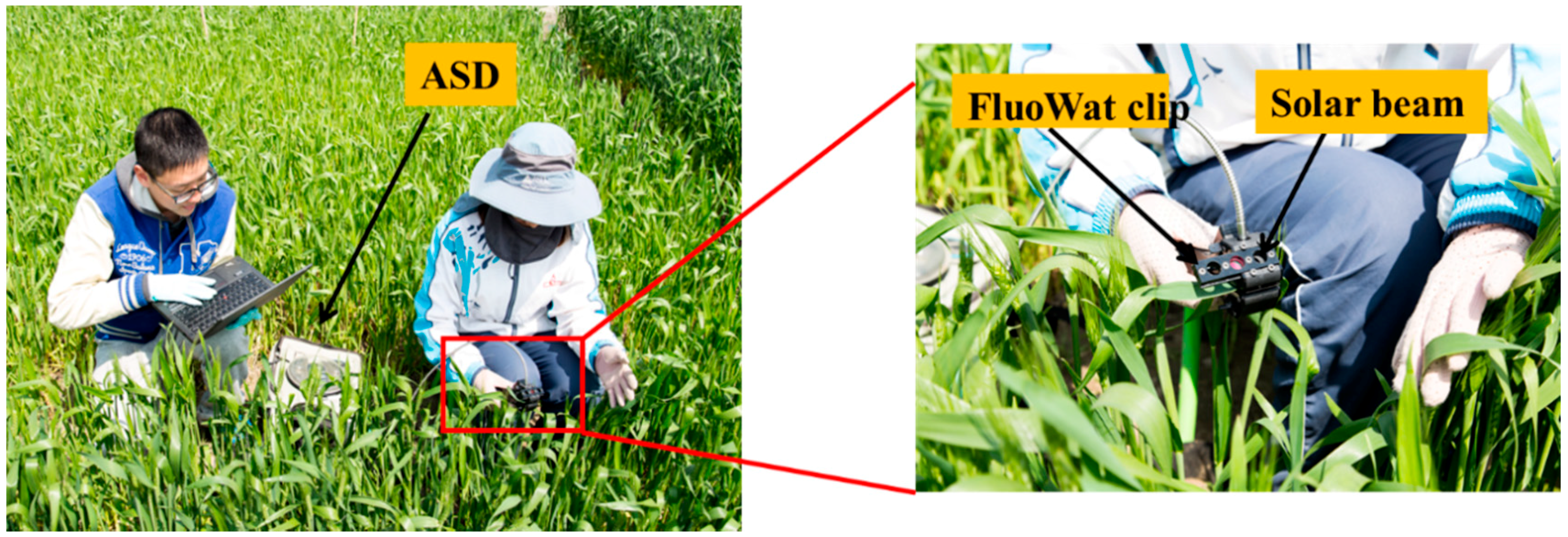
2.2. Measurements of Sun-Induced Fluorescence at the Leaf Scale

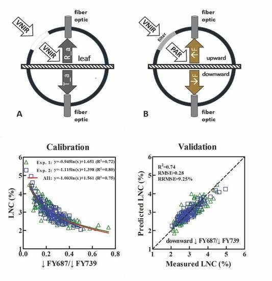
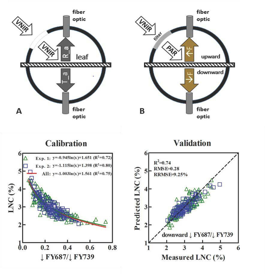
2.2.1. Acquisition of the Upward (↑F) and Downward (↓F) SIF Spectra at the Leaf Scale

Reflectance (R), transmittance (T) without fluorescence contribution, and chlorophyll fluorescence (F) datasets were measured under natural illumination with clear sky conditions using an ASD FieldSpec Pro FR2500 spectrometer (ASD) (Analytical Spectral Devices, Boulder, CO, USA) coupled with the FluoWat leaf clip (Producción por mecanizados villanueva S.L.U, Spain) from 10:00–11:30 at each growth stage [13,41,42]. The ASD recorded data at 1 nm intervals in the region of 350–2500 nm. The spectral data were collected with a sampling interval of 1.4 nm and a full width at half maximum (FWHM) spectral resolution of 3 nm in 350–1000 nm. It recorded reflectance with a sampling interval of 2 nm and a FWHM spectral resolution of 10 nm in 1000–2500 nm.
Due to the flexible design of the FluoWat leaf clip, fiber can be vertically positioned onto the adaxial and abaxial leaf (Figure 1A). The incoming sun radiance (I) was measured as the reflected radiance of a Spectralon reflectance standard (ODM-98, Gigahertz-Optik GmbH, Türkenfeld, Germany). When the leaf was clamped into the FluoWat leaf clip, the incident solar beam could be manually aligned into the open aperture with the direction of 45° relative to the leaf surface, and the R-T-F datasets were measured. Then, a high performance low pass filter (<650 nm, Producción por mecanizados villanueva S.L.U, Spain) was used to cut off the light above 650 nm, the upward and downward fluorescence emission (↑F and ↓F) were obtained separately (Figure 1B) [13,42]. Upward and downward sun-induced fluorescence emission (↑F and ↓F) were measured at the same point of the upper and lower epidermis of the wheat leaf, respectively. The point of the measurement was at two-thirds of the distance from the leaf base. The first, second, and third fully-expanded leaves from the top were selected randomly from a plant in every plot. The leaf veins were avoided to appear in the detection area during the measurements. Additional details regarding the data acquisition are provided in Figure 1 and Figure 2.

2.2.2. Sun-Induced Fluorescence (SIF) Yield Indices

Since the intensity of the incident light was different on every testing day during the whole wheat growth stages, SIF yield indices (FY, unitless) were calculated by normalizing the SIF for the absorbed incoming photosynthetic active radiance (APAR). APAR equals the integration of incoming sun radiance in the photosynthetic active radiation (PAR) region (400–700 nm) multiplying with the fraction of the light absorbed in the PAR region of (fAPAR) [42] (Equations (1)–(5)). The total measured Chl fluorescence yield (FYtot, unitless) equals the sum of the upward and downward Chl fluorescence yield (FYtot = ↑FY + ↓FY). Additionally, several SIF yield indices constructed by the red and the far-red emission peaks also were calculated to track the characteristics of the SIF spectra (Table 2). More details about the measurements and the formulas of SIF yield indices used in the paper, can be seen in [13,42].
  PAR = 400 700 I d λ  
  fAPAR = ( 1 R T )  
  APAR = 400 700 [   I × fAPAR ] d λ  
  FY = F APAR  
  FY = F APAR  
The distribution of SIF peaks in the red region and far-red region was close to the normal distribution, as shown in Figure 3. The data collected from the two ecological sites showed that the peak in the red region was located in the range of 685–690 nm, among which a 40% SIF peak appeared at 687 nm (Figure 3A). The peak in the far-red region was situated around 735–741 nm, of which a 58% SIF peak was discovered at 739 nm (Figure 3B). Therefore, the SIF yield indices calculated in this study were based on the peak emission positions of 687 nm and 739 nm.

2.3. Measurements of Leaf Biochemical Parameters

All leaves were detached for scanning and weighing after the measurement of SIF. Leaf area was determined with a leaf area meter LI-3000 (LI-COR, Inc., Lincoln, NE, USA). Finally, leaves were oven-dried at 105 °C for 30 min, and then at 80 °C for 48 h until a constant dry weight (DW) was obtained. LMA was calculated as grams of dry mass per square centimeter. The LNC in the leaf tissues (% or Gn·g−1 DW) was determined using the micro-Kjeldahl method in this study. The leaf Chl content was estimated by the PROCWT model which couples PROSPECT with continuous wavelet transform [43].

2.4. Calculation of Vegetation Indices

To compare the differences in detection of LNC between the SIF and the vegetation indices, some widely used vegetation indices from previous studies are cited, such as a normalized difference vegetation index (NDVI), enhanced vegetation index (EVI2), red edge inflection point (REP), green NDVI, green chlorophyll index (CIgreen), and red edge chlorophyll index (CIred edge). NDVI, EVI2, and green NDVI are generally applied for the remote estimation of canopy LAI, while REP, CIgreen, and CIred edge are widely used to estimate the Chl content. The detailed information is summarized in Table 3.

2.5. Statistical Analysis

The constructed models of combined wheat LNC data were evaluated in leave-one-out cross validation (LOOCV). The predictive performance of LNC models on SIF yield indices was evaluated using different statistical parameters: The coefficient of determination (R2); root mean square error (RMSE); relative root mean square error (RRMSE).
The fitness between the predicted and observed values were evaluated by the square of correlation coefficient (R2), the root mean square error (RMSE) [50], and relative root mean square error (RRMSE) [51].

3. Results

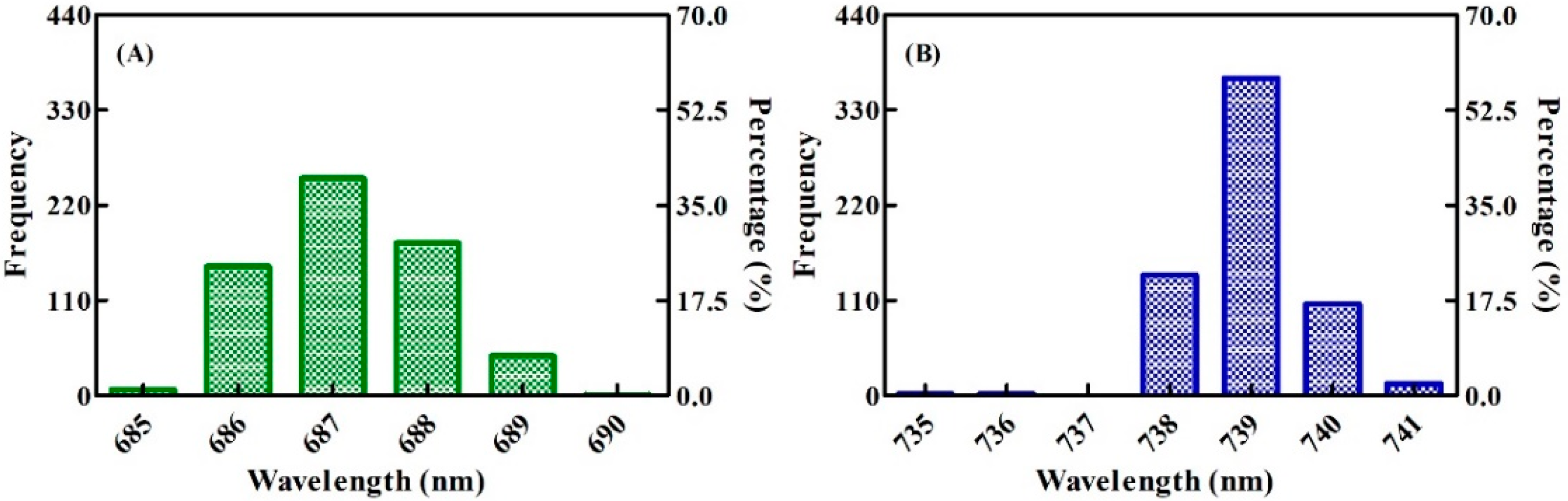
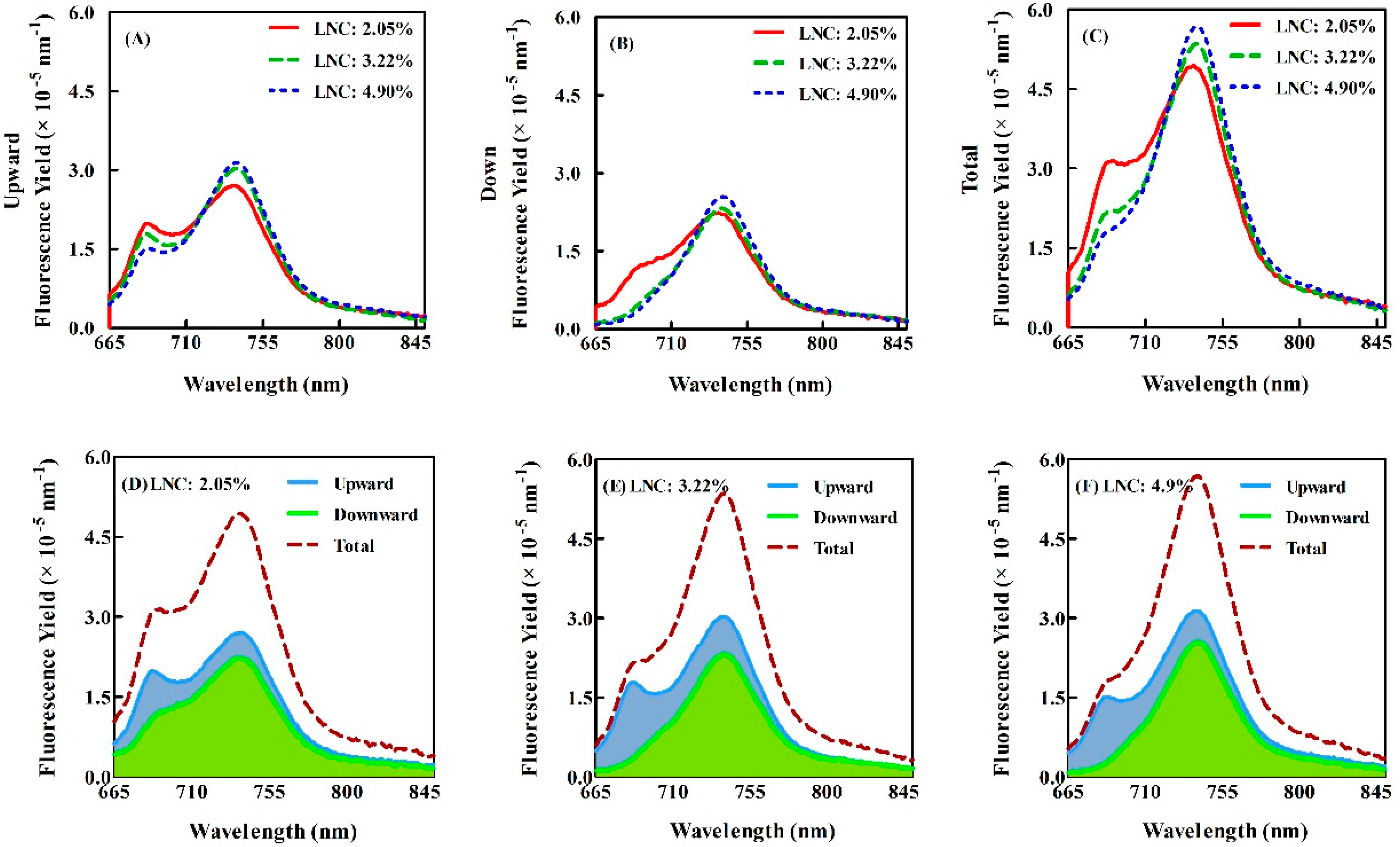
3.1. Characteristics of SIF Spectra at the Leaf Scale under Varied Nitrogen Rates

We took the Experiment 2 data as the example to demonstrate the differences of the downward and upward SIF in the region of 665–850 nm at different nitrogen levels (Figure 4), and SIF in the region of 650–665 nm was deleted due to the noise of partial transmittance of the filter in the region. Generally, Figure 4A–C show that, with the increase of LNC, SIF yield is decreasing in the red region, while it rises in the near-infrared region, which was observed on both the upward and downward SIF yield. The red and far-red peaks are clearly visible at the upward SIF spectra, with a lower peak in the red region than that in the far-red region (Figure 4A); but, in the downward SIF yield spectrum, the red peak is inconspicuous, especially for the leaves with high LNC (Figure 4B).
Figure 4D–F show how the signal of the downward SIF is generally weaker than that of the upward SIF for a given LNC. Both the signal of two peaks in the red region and the far-red region for the downward SIF is significantly smaller than that in the upward SIF. However, the peak in the far-red region is only a little smaller in downward SIF than that in the upward SIF. The changing trend was consistent under the different nitrogen levels.

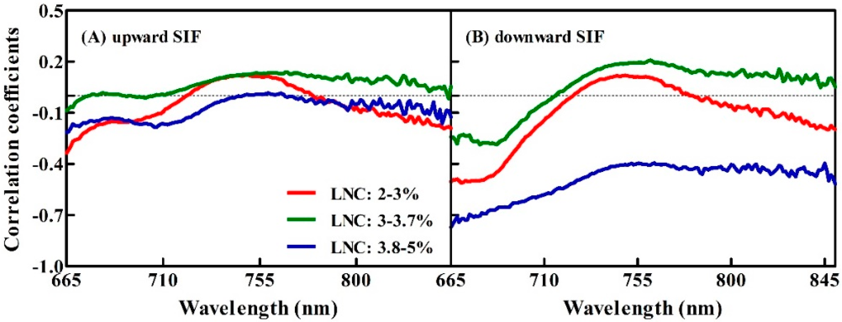
3.2. Correlations between the Upward and Downward SIF Yield and Three Given LNC Ranges for the Winter Wheat

Correlation coefficients between the upward and downward SIF yield spectra and the three different ranges of LNC are shown in Figure 5. It shows that the sensitive band to the LNC is approximately at 686 nm in the visible spectral range. There is a quite flat curve in the region of 730–770 nm in the far-red region, with the close to highest correlation with LNC at 758 nm for both upward and downward SIF, as shown in Figure 5. The LNC is negatively correlated to both upward and downward SIF of wheat leaves in the region of 650–720 nm, which shows similar trends in different bands under all the LNC ranges. However, the correlation coefficient in the region of 720–830 nm is positive when the LNC was <3.8% for bidirectional SIF, nevertheless, it is negative in the region of 650–850 nm when 3.8% < LNC < 5% for the downward SIF (Figure 5B). Overall, the downward SIF exhibits a closer relationship with the LNC than that of the upward SIF for the whole SIF region, especially when the LNC is >3.8%. Meanwhile, the correlation coefficient between the LNC and SIF is significantly higher in the red region than that in the far-red region, especially when LNC is <3.8%.

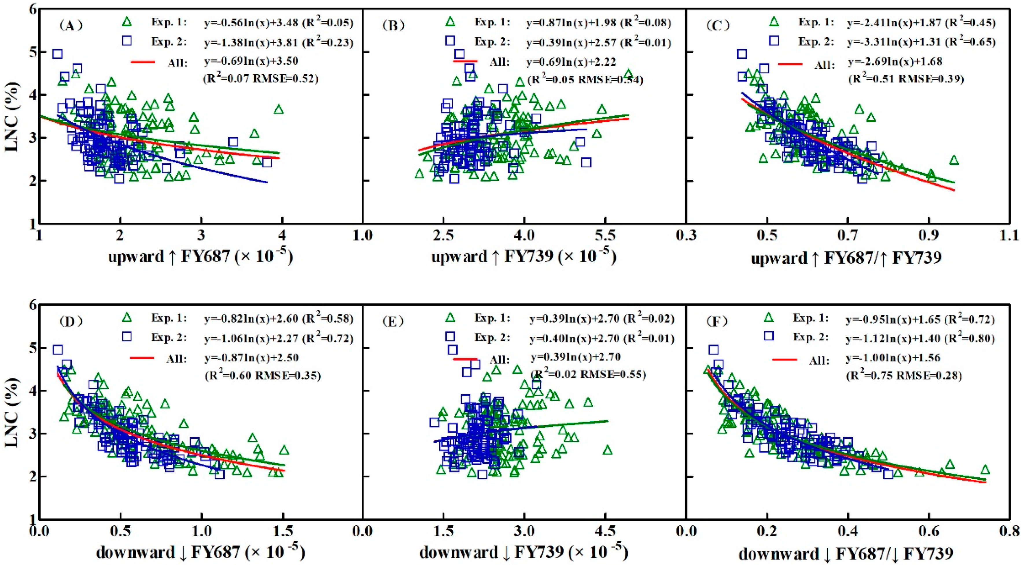
3.3. Constructing the LNC Estimation Models on SIF Yield Indices in Wheat

The scatter plots for the 210 pairs of the LNC and the upward and downward SIF yield indices samples for two experiments (Experiment 1 and Experiment 2) are shown in Figure 6. The best-fit function for the relationships between SIF yield indices and the LNC are all nonlinear. It shows that ↓FY687 performs much better than ↑FY687 with R2 as 0.58, 0.72 and 0.60 for Experiment 1, Experiment 2 and combined datasets, respectively (Figure 6A,D). Neither the upward nor downward FY739 indices present any correlation (Figure 6B,D). The upward red/far-red peak ratios (↑FY687/↑FY739) yield the performance with R2 values of 0.45, 0.65, and 0.51 for Experiment 1, Experiment 2, and combined data, respectively. The downward red/far-red peak ratio ↓FY687/↓FY739 exhibits the strongest relationship with a non-linear character in each dataset (R2 = 0.72, 0.80 and 0.75 for Experiment 1 dataset, Experiment 2 dataset, and combined, respectively) (Figure 6F).
Figure 6A–C show that, for all upward SIF yield indices, the upward red/far-red peak ratio index ↑FY687/↑FY739 has better fit with the LNC, although with an R2 of 0.65 it is not very strong. Among the downward SIF yield indices, the ratio ↓FY687/↓FY739 has the best ability to estimate the LNC due to the highest fit, in this case, with an R2 between 0.72 and 0.80. Briefly, ↓FY687, ↑FY687/↑FY739 and ↓FY687/↓FY739 yield better results with LNC than other SIF yield indices. However, it seems that these three SIF yield indices lack sensitivity to the LNC at low LNC values.
To conclude, the best-fit functions for the relationships between SIF yield indices and LNC were mostly nonlinear with better performance in downward SIF yield indices than that of the upward ones. The red/far-red peak ratio indices showed higher correlation with LNC than that of the single peak SIF yield indices, particularly for ↓FY687/↓FY739 on which the nonlinear exponent prediction function was built with the best goodness of fit. Moreover, it was also found that the differences of the ↓FY687/↓FY739 models between the two data sets were the smallest.

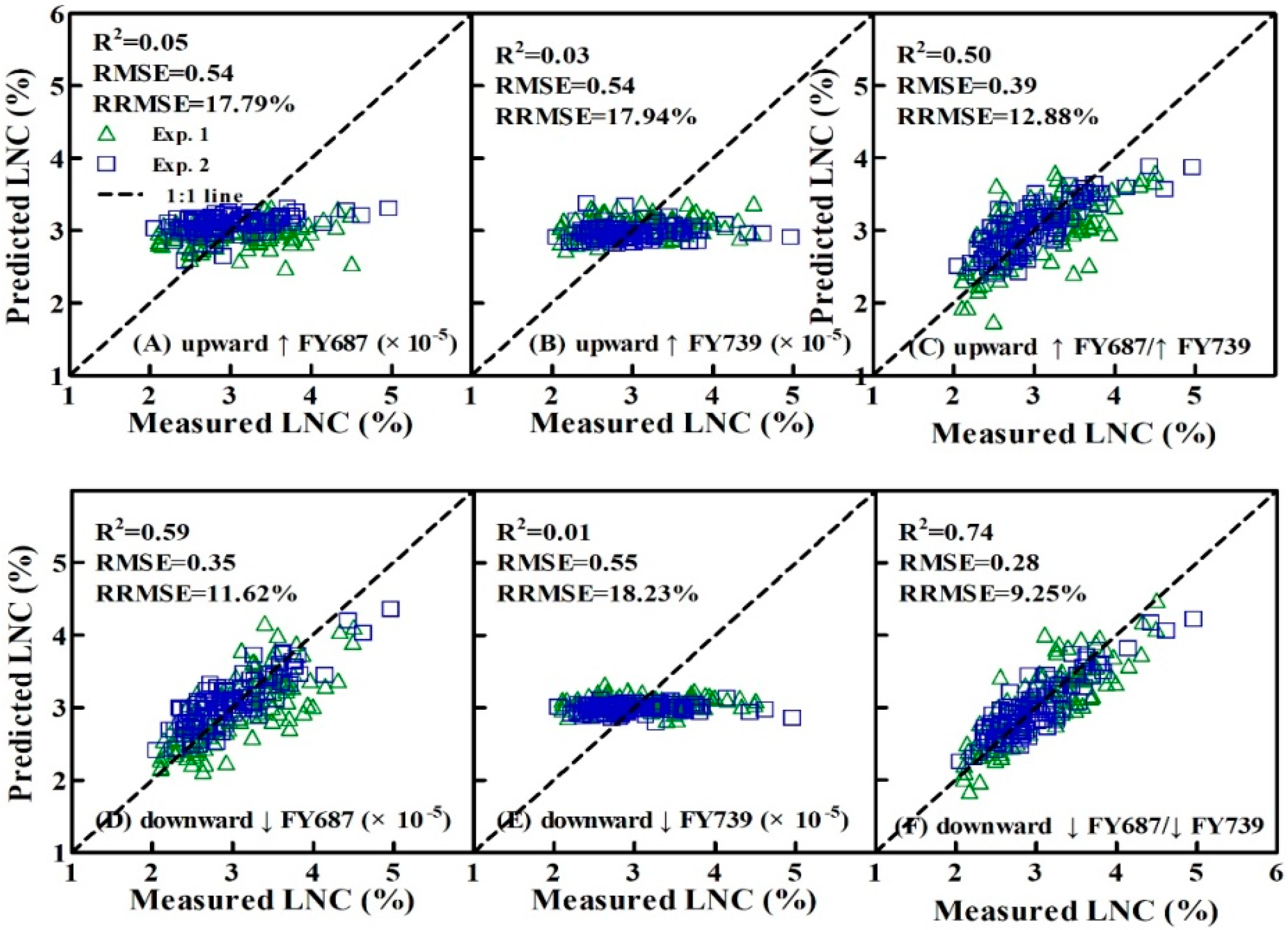
3.4. Validation of the Estimated LNC Model on SIF Yield Indices in Wheat

The LNC models constructed on the upward and downward SIF yield indices group of FY687, FY739 and red/far-red peak ratio indices (FY687/FY739) were validated by the two combined datasets using LOOCV with three statistical parameters of the coefficients of determination (R2), the root mean square error (RMSE) and relative root mean square error (RRMSE) (Figure 7). Among them, the estimation models built on ↓FY687 and red/far-red peak ratio indices group (↑FY687/↑FY739 and ↓FY687/↓FY739) performed well overall (Figure 7C,D,F). Additionally, ↓FY687/↓FY739 did best with the highest correlation (0.74) and the lowest RRMSE (9.25%), followed by ↑FY687/↑FY739 (R2 = 0.50, RMSE = 0.39, RRMSE = 12.88%). The regression line was close to y = x line. The 1:1 plotting with the observed and predicted values exhibited the reliability and accuracy of the derived models, as shown in Figure 7C,F.
Table 4 illustrates the performance of monitoring models for LNC on vegetation indices used in previous studies for 210 combined samples. Based on the statistical parameters of the calibration and validation sets, CIred edge shows the highest correlation to LNC, followed by CIgreen, Green NDVI, and REP, which yielded better precision than NDVI and EVI for LNC detection. Consistent with the performance in calibration, NDVI and EVI show poorer accuracy than the other four vegetation indices. The vegetation indices NDVI and EVI used for estimation of LAI did not perform well since they were not sensitive when the LNC was high. Compared with the SIF yield indices, only downward fluorescence ratios (↓FY687/↓FY739) appeared to perform better than CIred edge, but not significantly.

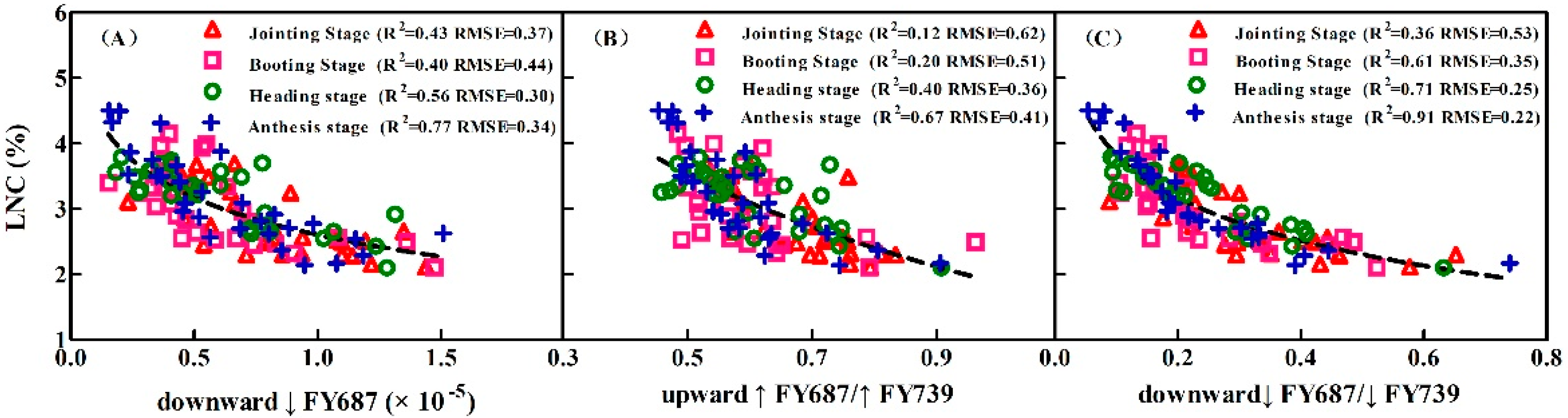
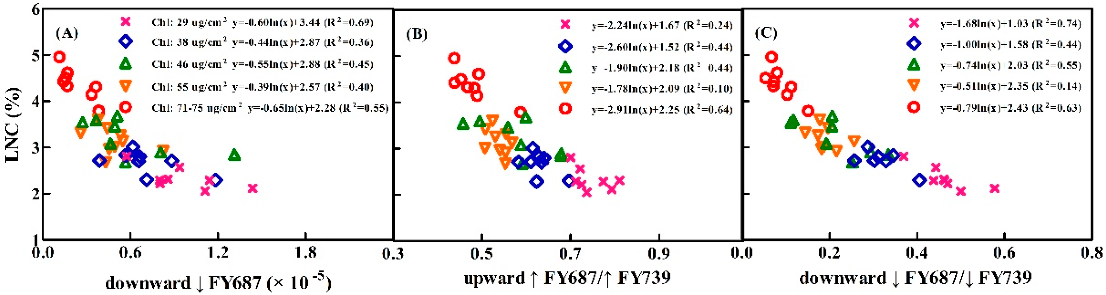
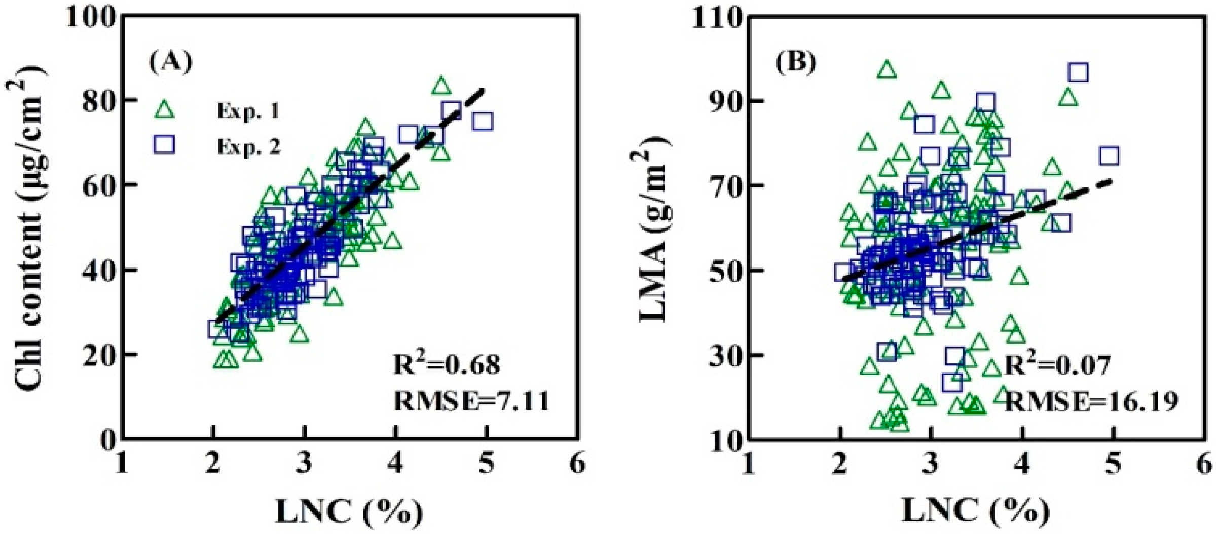
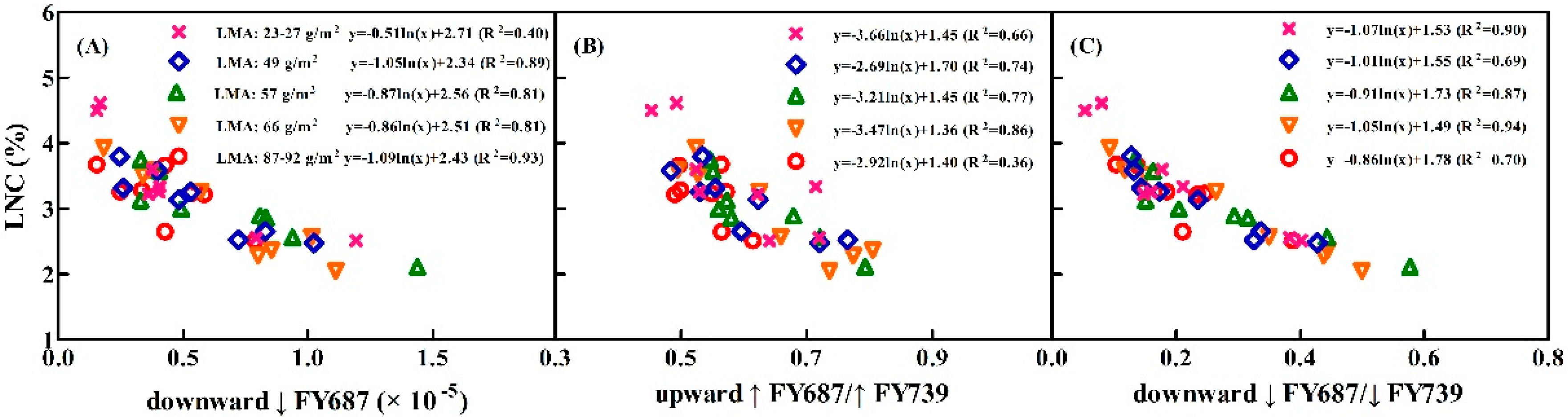
3.5. Assessing the LNC Models on SIF Yield Indices under Individual Stage, Different LNC, Chl Content, and Leaf Structure LMA

It can be seen that ↓FY687, ↑FY687/↑FY739, and ↓FY687/↓FY739 yield stable relationships with LNC under various stages with broader ranges of Chl content, in Figure 6. Due to the more complete data acquisition period in Experiment 1 than that of Experiment 2, we took Experiment 1 as the example to compare the performance of these three LNC models in individual stages (Figure 8). They all had the best performance during the anthesis stage, followed by the heading stage, booting stage, and jointing stage. This might be caused by the large difference among the samples at the anthesis stage, which led to the wide range of LNC, Chl content and leaf-structure properties. Meanwhile, the range of ↓FY687/↓FY739 and ↓FY687 were larger than ↑FY687/↑FY739, therefore, the LNC models based on ↓FY687/↓FY739 and ↓FY687 have stronger applicability.
SIF emission is influenced by the re-absorption of Chl and leaf structure. The data of the LNC and SIF were divided into five groups according to the value of Chl content and LMA in this study. The objective was to evaluate LNC models on the conditions of practical growth status with varied Chl content and LMA. Figure 9 shows the scatter diagram of SIF yield indices and LNC at different Chl content levels. Observing the Chl content at different groups, the distribution of SIF–LNC scatter changed a little with the change of Chl content. Especially when Chl content is about 55 μg·cm−2, the ↑FY687/↑FY739 and ↓FY687/↓FY739 were not sensitive to LNC. The SIF yield indices ↓FY687 and ↓FY687/↓FY739 still were sensitive to LNC under the low Chl concentrations, just the model changed a little. Generally, the changes of the SIF–LNC models in five groups were not significant. As shown in Figure 10A, although Chl was highly related to LNC, Chl content exerted influence on the relationships between ↓FY687, ↑FY687/↑FY739, and ↓FY687 and the LNC.
We explored the LMA impact on the relationship between SIF yield indices and the LNC with a sensitivity analysis using some measured data with different LMA categories (Figure 11). All the SIF yield indices showed less variability to LMA (Figure 11) for LMA values in each range (14–97 g/m2) and all LNC ranges (1–5%). SIF were sensitive to LNC all the time and the relationships between SIF and LNC at five groups hardly changed. Therefore, the relationships between all SIF yield indices and LNC were almost independent of the LMA. Meanwhile, Figure 10B shows that the LMA is not relevant to LNC in any case. It can be concluded that the SIF emission also is affected by other leaf properties.

4. Discussion

4.1. Power of the Upward and Downward SIF Yield Indices (↑FY and ↓FY) in LNC Detection

This study showed that the absolute value of upward SIF emission was higher than that of the downward SIF for all leaves. Figure 12A,B,C also show that the value of the downward SIF yield indices (↓FY687 and ↓FY739) are generally lower than that in the upward fluorescence (↑FY687 and ↑FY739). Due to the stronger absorption, scattering effect for the SIF emission [52], and more chlorophyll content around the upper epidermis, it was observed that the upward SIF radiance and SIF yield indices were higher compared with that of the downward SIF, especially for the SIF peak in the red region, which is consistent with [40,53]. Much of the light is absorbed by the palisade parenchyma, in the view of light propagation in the leaves. The SIF emitted downward possibly was self-absorbed a second time by Chl in the leaf, reducing the downward SIF, which was weaker with the spongiform parenchyma acting as a diffuser [54].
Since the LNC is directly linked to Chl content, it is to be expected that the emission of the peak in the red region decreased with the increasing of the LNC, however, increased in the far-red region. This phenomenon of the transmittance and reflectance characteristics for wheat leaves was consistent with the upward and downward SIF, which is the same as the previous results [55,56,57]. The reason for the low accuracy of ↑FY739 and ↓FY739 for the LNC is the strong self-absorption of chlorophyll in the red region rather than in the far-red region. The red peak of SIF is more likely to be closely correlated to the LNC than the far-red peak, which agrees with previous study [52]. Although the downward SIF signal was weaker than that of the upward SIF, the correlation coefficient between the LNC and the downward SIF was higher than that with the upward SIF. Bidirectional observations revealed that downward SIF yield indices (↓FY687 and ↓FY687/↓FY739), ↓FY687/↓FY739 especially has a closer relationship with the LNC than that with the upward SIF yield indices (↑FY687 and ↑FY687/↑FY739) (Figure 5 and Figure 6). Zhao et al. [53] also indicated that the downward SIF was more sensitive to Chl content than the upward SIF in the red region by the sensitivity analysis. The cause for these phenomena might be the absorption of Chl, which was more obvious for the downward SIF than that for the upward SIF [58,59]. Moreover, this effect can also be influenced by the leaf thickness, which will affect the photon’s path length within the leaf [53]. Van Wittenberghe [13] concluded that the downward SIF, as an important part of SIF emission, should be taken into consideration when interpreting the SIF signal at the scales of leaf, canopy, and landscape, which validates the results of this study.

4.2. Reason for Better Performance of Peak Ratio Indices in LNC Detection

Compared with the single peak SIF yield indices, the red/far-red peak ratio indices (↑FY687/↑FY739, ↓FY687/↓FY739) reflected the proportion of two photosystems. Regarding the two peaks in the SIF, the peak located in the red spectral region (around 687 nm) mainly originated from Photosystem II (PS II), and the other peak (about 739 nm) in the far-red region attributed to both Photosystem I (PS I) and PS II [29,30]. The reason for the better performance of red/far-red peak ratio in LNC estimation is not only the stacking of the thylakoid membranes, but also the associated changes in spillover [60], led to the red/far-red peak ratio performing better in detecting several types of growth status. According to the relevant studies over the last decades, it has been verified that the red/far-red peak ratio index (F687/F739) from active fluorescence technology is correlated with the maximum photochemical efficiency of PS II, largely due to reabsorption in the red region for ChlF, which was suggested to be an indicator to Chl content [61,62], especially in diagnosing the plant stress status [63]. Van Wittenberghe et al. [13] found that both the red/far-red peak ratio indices (↓FY (687)/↓FY (741) and ↑FY (687)/↑FY (739)) have a high correlation with Chl content, and they decrease with the increasing of Chl content. According to Tubuxin et al. [37], solar-induced and artificial light-induced Chl fluorescence yield ratios of 686 nm and 760 nm were both highly correlated with the Chl content. Due to the strong relationship between Chl content and LNC, the red/far-red peak ratio indices (↑FY687/↑FY739, ↓FY687/↓FY739) could be used to estimate the LNC, especially for the downward SIF yield indices ↓FY687/↓FY739, which also corresponded well with the result drawn by [22,23,24].
It can be seen that ↓FY687, ↑FY687/↑FY739, and ↓FY687/↓FY739 all lacked sensitivity to the LNC at low LNC values. Since the LNC models constructed in this study were empirical, inevitably there would be a problem on the high value or low value. Figure 6 shows that, although the SIF yield indices might lack sensitivity to those parameters of the LNC at low LNC values, it displays that the relationships between ↓FY687, ↓FY687/↓FY739, and LNC—shown in Figure 9A,B—were better than expected. The SIF yield indices ↓FY687 and ↓FY687/↓FY739 still were sensitive to the LNC under the low Chl concentrations, which changed a little compared to the model built on all data.
Generally, simpler methods (SPAD, Dualex) are preferred to estimate the LNC [64,65], however, neither can be used at the leaf scale. Although the reflectance-based parameters are widely used to monitor LNC [66], they lack specificity to nitrogen stress [12]. Compared with the performance of vegetation indices, only the result yielded by the downward fluorescence ratio (↓FY687/↓FY739) was better than CIred edge, while the relationships between other SIF yield indices and the LNC was not as good as CIred edge. This might be because the LNC used in this paper refers to the total nitrogen, including the nitrogen involved in photosynthesis and nitrogen in other forms. SIF mainly monitors the nitrogen which is involved in photosynthesis. The mechanism of SIF for the LNC estimation is different from that of hyperspectral remote sensing, which is based on the spectral absorption characteristics caused by the chemical bonds in the chemical composition under certain light intensities. The RubisCo and the Chl are two major storage for nitrogen, both of which are involved in photosynthesis. Evans [67] found that, within species, there are strong linear relationships between nitrogen and both RuBP carboxylase and chlorophyll. Since Chl can be measured easily, in this study only the Chl was taken into consideration, which could be the reason the monitoring accuracy was not very high.

4.3. Performance of the Relationships between SIF Yield Indices and LNC under the Varied Chl Content and Leaf Structure LMA

The influence of the Chl content and the LMA on the LNC models was explored using the field-measured datasets. Chl content is a significant factor in linking SIF with LNC, so the conclusion of this study can provide a reference for LNC estimation using SIF yield indices. The SIF yield indices seemed to be less accurate at a lower LNC content. Regarding low Chl content, the slopes of ↓FY687, ↓FY687/↓FY739, and LNC were still sensitive, however, the SIF–LNC model changed a little, including the slope and intercept. Zhang et al. [39] also found that the slope of gross primary production and SIF also was insensitive when Cab was >20 μg∙cm–2 using the model-based analysis.
We did not record leaf angle and leaf thickness, so the LMA was the alternative for leaf structure. This study showed that the relationships between SIF yield indices and LNC were relatively insensitive to the LMA. Van Wittenberghe et al. [13] illustrated there was not a significant influence of specific leaf area on ↓F755/↑F755. The result probably was caused by the emission fluorescence escaped from the leaf being affected by the other properties, such as the pigments and leaf structure., To reduce the influence of variable light intensity, the SIF yield indices used in the study were normalized by APAR, Therefore, regardless of saturated or unsaturated light conditions, the effects of light were minimized, meanwhile, the kinetic effects of the non-saturating light and the variability of chloroplast movement were not considered for the SIF measurement collected under variable light intensities. Therefore, in the ongoing research, we would focus on improving the machine for SIF measurement at the leaf scale and providing a more practical SIF index to estimate the LNC combining the result of canopy scale and assessing the influence of canopy structure properties (leaf area, leaf angle, and more) on the SIF yield indices.

5. Conclusions

We assessed the capacity of upward and downward SIF yield indices for LNC estimation at the leaf scale under various growth stages for winter wheat. The signal of the upward SIF was higher than that of the downward SIF due to the re-absorption and scattering effect. Bidirectional observations revealed that downward SIF had the higher fitness with the LNC than that of upward SIF. Downward SIF also played an important role for predicting the LNC of winter wheat. The downward red/far-red peak ratio index (↓FY687/↓FY739) showed the highest correlation to LNC with stable performance. The relationships between LNC and these three SIF yield indices (↓FY687, ↑FY687/↑FY739, and ↓FY687/↓FY739) were hardly influenced by the LMA and Chl content. Therefore, SIF can be used as a new priority with higher accuracy than vegetation indices to detect nitrogen content directly for future study in the scales of field and region. SIF can be affected by the canopy structure, background, and atmospheric absorption, but, in this study we simply assessed the LNC using SIF yield indices under the varied ranges of Chl content and LMA. We should consider the impact of those factors on LNC estimation by SIF yield indices in their on-going research.

Author Contributions

M.J., W.C., and X.Y. conceived and designed the research. M.J., J.Z., and C.M. contributed significantly to the field experiments and data collection. M.J., L.A., W.C., and X.Y. made important contributions to the research method, data analysis, and manuscript revision. D.L. provided the model PROCWT and contributed to retrieve chlorophyll content. T.C., Y.T., and Y.Z. contributed in providing suggestions for the research method, and data analysis.

Funding

This research was funded by the National Key Research and Development Program of China (2016YFD0300601), the National Natural Science Foundation of China (31671582), Jiangsu Distinguished Professor Program, Jiangsu Collaborative Innovation Center for Modern Crop Production, the Priority Academic Program Development of Jiangsu Higher Education Institutions (PAPD), and Qinghai Project of Transformation of Scientific and Technological Achievements (2018-NK-126), China.

Acknowledgments

We are thankful to Jose Moreno of the Image Process Laboratory in Valencia for providing the FluoWat leaf clip. We would also like to express our appreciation for the advice given by Liangyun Liu of Chinese Academy of Science, Yongguang Zhang of Nanjing University, and Feng Zhao of Beihang University. We are grateful to the reviewers for their suggestions and comments which significantly improved the quality of this paper.

Conflicts of Interest

The authors declare no conflict of interest.

References

  1. Clevers, J.; Gitelson, A.A. Remote estimation of crop and grass chlorophyll and nitrogen content using red-edge bands on Sentinel-2 and -3. Int. J. Appl. Earth Obs. Geoinf. 2013, 23, 344–351. [Google Scholar] [CrossRef]
  2. Miao, Y.; Mulla, D.J.; Hernandez, J.A.; Wiebers, M.; Robert, P.C. Potential impact of precision nitrogen management on corn yield, protein content, and test weight. Soil Sci. Soc. Am. J. 2007, 71, 1490–1499. [Google Scholar] [CrossRef]
  3. Diacono, M.; Rubino, P.; Montemurro, F. Precision nitrogen management of wheat: A review. Agron. Sustain. Dev. 2013, 33, 219–241. [Google Scholar] [CrossRef]
  4. Yang, J.; Gong, W.; Shi, S.; Du, L.; Sun, J.; Song, S. Estimation of nitrogen content based on fluorescence spectrum and principal component analysis in paddy rice. Plamt Soil Environ. 2016, 62, 178–183. [Google Scholar] [CrossRef] [Green Version]
  5. Inoue, Y.; Sakaiya, E.; Zhu, Y.; Takahashi, W. Diagnostic mapping of canopy nitrogen content in rice based on hyperspectral measurements. Remote Sens. Environ. 2012, 126, 210–221. [Google Scholar] [CrossRef]
  6. Yao, X.; Ren, H.; Cao, Z.; Tian, Y.; Cao, W.; Zhu, Y.; Cheng, T. Detecting leaf nitrogen content in wheat with canopy hyperspectrum under different soil backgrounds. Int. J. Appl. Earth Obs. Geoinf. 2014, 32, 114–124. [Google Scholar] [CrossRef]
  7. Yao, X.; Huang, Y.; Shang, G.; Zhou, C.; Cheng, T.; Tian, Y.; Cao, W.; Zhu, Y. Evaluation of Six Algorithms to Monitor Wheat Leaf Nitrogen Concentration. Remote Sens. 2015, 7, 14939–14966. [Google Scholar] [CrossRef] [Green Version]
  8. Schlemmer, M.; Gitelson, A.A.; Schepers, J.; Ferguson, R.; Peng, Y.; Shanahan, J.; Rundquist, D. Remote estimation of nitrogen and chlorophyll contents in maize at leaf and canopy levels. Int. J. Appl. Earth Obs. Geoinf. 2013, 25, 47–54. [Google Scholar] [CrossRef] [Green Version]
  9. Chen, P.; Haboudane, D.; Tremblay, N.; Wang, J.; Vigneault, P.; Li, B. New spectral indicator assessing the efficiency of crop nitrogen treatment in corn and wheat. Remote Sens. Environ. 2010, 114, 1987–1997. [Google Scholar] [CrossRef] [Green Version]
  10. Nguy-Robertson, A.; Gitelson, A.A.; Peng, Y.; Viña, A.; Arkebauer, T.; Rundquist, D. Green Leaf Area Index Estimation in Maize and Soybean: Combining Vegetation Indices to Achieve Maximal Sensitivity. Agron. J. 2012, 104, 1336–1347. [Google Scholar] [CrossRef]
  11. Clevers, J.G.P.W.; Kooistra, L. Using hyperspectral remote sensing data for retrieving canopy chlorophyll and nitrogen content. IEEE J. Sel. Top. Earth Obs. Remote Sens. 2012, 5, 574–583. [Google Scholar] [CrossRef]
  12. Tremblay, N.; Wang, Z.; Cerovic, Z.G. Sensing crop nitrogen status with fluorescence indicators: A review. Agron. Sustain. Dev. 2011, 32, 451–464. [Google Scholar] [CrossRef]
  13. Van Wittenberghe, S.; Alonso, L.; Verrelst, J.; Moreno, J.; Samson, R. Bidirectional sun-induced chlorophyll fluorescence emission is influenced by leaf structure and light scattering properties—A bottom-up approach. Remote Sens. Environ. 2015, 158, 169–179. [Google Scholar] [CrossRef]
  14. Govindjee, G. Chlorophyll Fluorescence: A Bit of Basics and History; Springer: Dordrecht, The Netherlands, 2004; pp. 1–41. [Google Scholar]
  15. Kuckenberg, J.; Tartachnyk, I.; Noga, G. Detection and differentiation of nitrogen-deficiency, powdery mildew and leaf rust at wheat leaf and canopy level by laser-induced chlorophyll fluorescence. Biosyst. Eng. 2009, 103, 121–128. [Google Scholar] [CrossRef]
  16. Cendrero-Mateo, M.P.; Moran, M.S.; Papuga, S.A.; Thorp, K.R.; Alonso, L.; Moreno, J.; Ponce-Campos, G.; Rascher, U.; Wang, G. Plant chlorophyll fluorescence: Active and passive measurements at canopy and leaf scales with different nitrogen treatments. J. Exp. Bot. 2016, 67, 275–286. [Google Scholar] [CrossRef] [PubMed]
  17. Kalaji, H.M.; Oukarroum, A.; Alexandrov, V.; Kouzmanova, M.; Brestic, M.; Zivcak, M.; Samborska, I.A.; Cetner, M.D.; Allakhverdiev, S.I.; Goltsev, V. Identification of nutrient deficiency in maize and tomato plants by invivo, chlorophyll a, fluorescence measurements. Plant Physiol. Biochem. 2014, 81, 16–25. [Google Scholar] [CrossRef] [PubMed]
  18. Živčák, M.; Olšovská, K.; Slamka, P.; Galambošová, J.; Rataj, V.; Shao, H.B.; Brestič, M. Application of chlorophyll fluorescence performance indices to assess the wheat photosynthetic functions influenced by nitrogen deficiency. Plant Soil Environ. 2014, 60, 210–215. [Google Scholar] [CrossRef] [Green Version]
  19. Živčák, M.; Olšovská, K.; Slamka, P.; Galambošová, J.; Rataj, V.; Shao, H.B.; Kalaji, H.M.; Brestič, M. Measurements of chlorophyll fluorescence in different leaf positions may detect nitrogen deficiency in wheat. Zemdirbyste-Agriculture 2014, 101, 437–444. [Google Scholar] [CrossRef]
  20. Yang, J.; Gong, W.; Shi, S.; Du, L.; Sun, J.; Song, S.; Chen, B.; Zhang, Z. Analyzing the performance of fluorescence parameters in the monitoring of leaf nitrogen content of paddy rice. Sci. Rep. 2016, 6, 28787. [Google Scholar] [CrossRef] [PubMed] [Green Version]
  21. Cartelat, A.; Cerovic, Z.G.; Goulas, Y.; Meyer, S.; Lelarge, C.; Prioul, J.L.; Barbottin, A.; Jeuffroy, M.H.; Gate, P.; Agati, G.; et al. Optically assessed contents of leaf polyphenolics and chlorophyll as indicators of nitrogen deficiency in wheat (Triticum aestivum L.). Field Crops Res. 2005, 91, 35–49. [Google Scholar] [CrossRef]
  22. Buschmann, C. Variability and application of the chlorophyll fluorescence emission ratio red/far-red of leaves. Photosynth. Res. 2007, 92, 261–271. [Google Scholar] [CrossRef] [PubMed]
  23. Gitelson, A.; Buschmann, C.; Lichtenthaler, H.K. The chlorophyll fluorescence ratio F735/F700 as an accurate measure of the chlorophyll content in plants. Remote Sens. Environ. 1999, 69, 296–302. [Google Scholar] [CrossRef]
  24. Lichtenthaler, H.K.; Hak, R.; Rinderle, U. The chlorophyll fluorescence ratio F690/F730 in leaves of different chlorophyll content. Photosynth. Res. 1990, 25, 295–298. [Google Scholar] [CrossRef] [PubMed]
  25. Rosema, A.; Zahn, H. Laser Pulse Energy Requirements for Remote Sensing of Chlorophyll Fluorescence. Remote Sens. Environ. 1997, 62, 101–108. [Google Scholar] [CrossRef]
  26. Zhang, Y.J.; Zhao, C.J.; Liu, L.Y.; Wang, J.H.; Wang, R.C. Chlorophyll Fluorescence Detected Passively by Difference Reflectance Spectra of Wheat (Triticum aestivum L.) Leaf. J. Integr. Plant Biol. 2005, 47, 1228–1235. [Google Scholar] [CrossRef]
  27. Porcar-Castell, A.; Tyystjarvi, E.; Atherton, J.; Van der Tol, C.; Flexas, J.; Pfundel, E.E.; Moreno, J.; Frankenberg, C.; Berry, J.A. Linking chlorophyll a fluorescence to photosynthesis for remote sensing applications: Mechanisms and challenges. J. Exp. Bot. 2014, 65, 4065–4095. [Google Scholar] [CrossRef] [PubMed]
  28. Rascher, U.; Alonso, L.; Burkart, A.; Cilia, C.; Cogliati, S.; Colombo, R.; Damm, A.; Drusch, M.; Guanter, L.; Hanus, J.; et al. Sun-induced fluorescence—A new probe of photosynthesis: First maps from the imaging spectrometer HyPlant. Glob. Chang. Biol. 2015, 21, 4673–4684. [Google Scholar] [CrossRef] [PubMed] [Green Version]
  29. Papageorgiou, G.C.; Govindjee, G. Chlorophyll a Fluorescence—A Signature of Photosynthesis; Springer: Dordrecht, The Netherlands, 2004; p. 818. [Google Scholar]
  30. Baker, N.R. Chlorophyll Fluorescence: A Probe of Photosynthesis In Vivo. Annu. Rev. Plant Biol. 2008, 59, 89–113. [Google Scholar] [CrossRef] [PubMed]
  31. Franck, F.; Juneau, P.; Popovic, R. Resolution of the Photosystem I and Photosystem II contributions to chlorophyll fluorescence of intact leaves at room temperature. BBA Bioenerg. 2002, 1556, 239–246. [Google Scholar] [CrossRef] [Green Version]
  32. Guanter, L.; Zhang, Y.; Jung, M.; Joiner, J.; Voigt, M.; Berry, J.A.; Frankenberg, C.; Huete, A.R.; Zarco-Tejada, P.; Lee, J.E.; et al. Global and time-resolved monitoring of crop photosynthesis with chlorophyll fluorescence. Proc. Natl. Acad. Sci. USA 2014, 111, E1327–E1333. [Google Scholar] [CrossRef] [PubMed] [Green Version]
  33. Liu, L.; Zhang, Y.; Jiao, Q.; Peng, D. Assessing photosynthetic light-use efficiency using a solar-induced chlorophyll fluorescence and photochemical reflectance index. Int. J. Remote. Sens. 2013, 34, 4264–4280. [Google Scholar] [CrossRef]
  34. Wagle, P.; Zhang, Y.; Jin, C.; Xiao, X. Comparison of solar-induced chlorophyll fluorescence, light-use efficiency, and process-based GPP models in maize. Ecol. Appl. 2016, 26, 1211–1222. [Google Scholar] [CrossRef] [PubMed]
  35. Ni, Z.; Liu, Z.; Huo, H.; Li, Z.L.; Nerry, F.; Wang, Q.; Li, X. Early Water Stress Detection Using Leaf-Level Measurements of Chlorophyll Fluorescence and Temperature Data. Remote Sens. 2015, 7, 3232–3249. [Google Scholar] [CrossRef] [Green Version]
  36. Zhao, F.; Guo, Y.; Huang, Y.; Reddy, K.N.; Zhao, Y.; Molin, W.T. Detection of the onset of glyphosate-induced soybean plant injury through chlorophyll fluorescence signal extraction and measurement. J. Appl. Remote Sens. 2015, 9, 097098. [Google Scholar] [CrossRef]
  37. Tubuxin, B.; Rahimzadeh-Bajgiran, P.; Ginnan, Y.; Hosoi, F.; Omasa, K. Estimating chlorophyll content and photochemical yield of photosystem II (PhiPSII) using solar-induced chlorophyll fluorescence measurements at different growing stages of attached leaves. J. Exp. Bot. 2015, 66, 5595–5603. [Google Scholar] [CrossRef] [PubMed]
  38. Du, S.; Liu, L.; Liu, X.; Hu, J. Response of Canopy Solar-Induced Chlorophyll Fluorescence to the Absorbed Photosynthetically Active Radiation Absorbed by Chlorophyll. Remote Sens. 2017, 9, 911. [Google Scholar] [CrossRef]
  39. Zhang, Y.; Guanter, L.; Berry, J.A.; Van der Tol, C.; Yang, X.; Tang, J.; Zhang, F. Model-based analysis of the relationship between sun-induced chlorophyll fluorescence and gross primary production for remote sensing applications. Remote Sens. Environ. 2016, 187, 145–155. [Google Scholar] [CrossRef]
  40. Louis, J.; Cerovic, Z.G.; Moya, I. Quantitative study of fluorescence excitation and emission spectra of bean leaves. J. Photochem. Photobiol. B 2006, 85, 65–71. [Google Scholar] [CrossRef] [PubMed]
  41. Alonso, L.; Gomez-Chova, L.; Vila-Frances, J.; Amoros-Lopez, J.; Guanter, L.; Calpe, J.; Moreno, J. Sensitivity analysis of the fraunhofer line discrimination method for the measurement of chlorophyll fluorescence using a field spectroradiometer. In Proceedings of the IEEE International Geoscience and Remote Sensing Symposium (IGARSS), Barcelona, Spain, 23–28 July 2007; pp. 3756–3759. [Google Scholar]
  42. Van Wittenberghe, S.; Alonso, L.; Verrelst, J.; Hermans, I.; Delegido, J.; Veroustraete, F.; Valcke, R.; Moreno, J.; Samson, R. Upward and downward solar-induced chlorophyll fluorescence yield indices of four tree species as indicators of traffic pollution in Valencia. Environ. Pollut. 2013, 173, 29–37. [Google Scholar] [CrossRef] [PubMed]
  43. Li, D.; Cheng, T.; Jia, M.; Zhou, K.; Lu, N.; Yao, X.; Tian, Y.; Zhu, Y.; Cao, W. PROCWT: Coupling PROSPECT with continuous wavelet transform to improve the retrieval of foliar chemistry from leaf bidirectional reflectance spectra. Remote Sens. Environ. 2018, 206, 1–14. [Google Scholar] [CrossRef]
  44. Rouse, J.W. Monitoring the Vernal Advancement and Retrogradation (Greenwave Effect) of Natural Vegetation; NASA/GSFCT Technical Report; NTRS: Chicago, IL, USA, 1974.
  45. Jiang, Z.; Huete, A.; Didan, K.; Miura, T. Development of a two-band enhanced vegetation index without a blue band. Remote Sens. Environ. 2008, 112, 3833–3845. [Google Scholar] [CrossRef]
  46. Guyot, G.; Baret, F. Utilisation de la Haute Resolution Spectrale pour Suivre L’etat des Couverts Vegetaux. Spectr. Signat. Objects Remote Sens. 1988, 287, 279. [Google Scholar]
  47. Gilabert, M.A.; Gandía, S.; Meliá, J. Analyses of spectral-biophysical relationships for a corn canopy. Remote Sens. Environ. 1996, 55, 11–20. [Google Scholar] [CrossRef]
  48. Gitelson, A.A.; Gritz, Y.; Merzlyak, M.N. Relationships between leaf chlorophyll content and spectral reflectance and algorithms for non-destructive chlorophyll assessment in higher plant leaves. J. Plant Physiol. 2003, 160, 271–282. [Google Scholar] [CrossRef] [PubMed]
  49. Gitelson, A.A.; Viña, A.; Ciganda, V.; Rundquist, D.C.; Arkebauer, T.J. Remote estimation of canopy chlorophyll content in crops. Geophys. Res. Lett. 2005, 32. [Google Scholar] [CrossRef]
  50. Cheng, T.; Riaño, D.; Ustin, S.L. Detecting diurnal and seasonal variation in canopy water content of nut tree orchards from airborne imaging spectroscopy data using continuous wavelet analysis. Remote Sens. Environ. 2014, 143, 39–53. [Google Scholar] [CrossRef]
  51. Gnyp, M.L.; Miao, Y.; Yuan, F.; Ustin, S.L.; Yu, K.; Yao, Y.; Huang, S.; Bareth, G. Hyperspectral canopy sensing of paddy rice aboveground biomass at different growth stages. Field Crops Res. 2014, 155, 42–55. [Google Scholar] [CrossRef]
  52. Zhao, F.; Guo, Y.; Huang, Y.; Verhoef, W.; Van der Tol, C.; Dai, B.; Liu, L.; Zhao, H.; Liu, G. Quantitative Estimation of Fluorescence Parameters for Crop Leaves with Bayesian Inversion. Remote Sens. 2015, 7, 14179–14199. [Google Scholar] [CrossRef] [Green Version]
  53. Vogelmann, T.C.; Han, T. Measurement of gradients of absorbed light in spinach leaves from chlorophyll fluorescence profiles. Plant Cell Environ. 2000, 23, 1303–1311. [Google Scholar] [CrossRef] [Green Version]
  54. Vogelman, T.C.; Nishio, J.N.; Smith, W.K. Leaves and light capture: Light propagation and gradients of carbon fixation within leaves. Trends Plant Sci. 1996, 1, 65–70. [Google Scholar] [CrossRef]
  55. Thomas, J.R.; Gausman, H.W. Leaf Reflectance vs. Leaf Chlorophyll and Carotenoid Concentrations for Eight Crops1. Agron. J. 1977, 69, 799–802. [Google Scholar] [CrossRef]
  56. Bauerle, W.L.; Weston, D.J.; Bowden, J.D.; Dudley, J.B.; Toler, J.E. Leaf absorptance of photosynthetically active radiation in relation to chlorophyll meter estimates among woody plant species. Sci. Hortic. 2004, 101, 169–178. [Google Scholar] [CrossRef]
  57. Wang, J.F.; He, D.X.; Song, J.X.; Dou, H.J.; Du, W.F. Non-destructive measurement of chlorophyll in tomato leaves using spectral transmittance. Int. J. Agric. Biol. Eng. 2015, 8, 73–78. [Google Scholar]
  58. Fournier, A.; Daumard, F.; Champagne, S.; Ounis, A.; Goulas, Y.; Moya, I. Effect of canopy structure on sun-induced chlorophyll fluorescence. ISPRS J. Photogramm. Remote Sens. 2012, 68, 112–120. [Google Scholar] [CrossRef]
  59. Middleton, E.M.; Cheng, Y.B.; Corp, L.A.; Campbell, P.K.E.; Huemmrich, K.F.; Zhang, Q.; Kustas, W.P. Canopy level Chlorophyll Fluorescence and the PRI in a cornfield. In Proceedings of the IEEE International Geoscience and Remote Sensing Symposium (IGARSS), Munich, Germany, 22–27 July 2012; pp. 7117–7120. [Google Scholar]
  60. Butler, W.L.; Kitajima, M. Energy transfer between Photosystem II and Photosystem I in chloroplasts. Biochim. Biophys. Acta 1975, 396, 72–85. [Google Scholar] [CrossRef]
  61. Hák, R.; Lichtenthaler, H.K.; Rinderle, U. Decrease of the chlorophyll fluorescence ratio F690/F730 during greening and development of leaves. Radiat. Environ. Biophys. 1990, 29, 329–336. [Google Scholar] [CrossRef] [PubMed]
  62. Pedrós, R.; Goulas, Y.; Jacquemoud, S.; Louis, J.; Moya, I. FluorMODleaf: A new leaf fluorescence emission model based on the PROSPECT model. Remote Sens. Environ. 2010, 114, 155–167. [Google Scholar] [CrossRef] [Green Version]
  63. Rossini, M.; Meroni, M.; Celesti, M.; Cogliati, S.; Julitta, T.; Panigada, C.; Rascher, U.; Van der Tol, C.; Colombo, R. Analysis of Red and Far-Red Sun-Induced Chlorophyll Fluorescence and Their Ratio in Different Canopies Based on Observed and Modeled Data. Remote Sens. 2016, 8, 412. [Google Scholar] [CrossRef]
  64. Errecart, P.M.; Agnusdei, M.G.; Lattanzi, F.A.; Marino, M.A. Leaf nitrogen concentration and chlorophyll meter readings as predictors of tall fescue nitrogen nutrition status. Field Crops Res. 2012, 129, 46–58. [Google Scholar] [CrossRef]
  65. Li, J.W.; Zhang, J.X.; Zhao, Z.; Lei, X.D.; Xu, X.L.; Lu, X.X.; Weng, D.L.; Gao, Y.; Cao, L.K. Use of fluorescence-based sensors to determine the nitrogen status of paddy rice. J. Agric. Sci. 2013, 151, 862–871. [Google Scholar] [CrossRef]
  66. Li, F.; Miao, Y.; Hennig, S.D.; Gnyp, M.L.; Chen, X.P.; Jia, L.L.; Bareth, G. Evaluating hyperspectral vegetation indices for estimating nitrogen concentration of winter wheat at different growth stages. Precis. Agric. 2010, 11, 335–357. [Google Scholar] [CrossRef]
  67. Evans, J.R. Photosynthesis and nitrogen relationships in leaves of C3 plants. Oecologia 1989, 78, 9–19. [Google Scholar] [CrossRef] [PubMed] [Green Version]
Figure 1. Scheme of the FluoWat leaf clip during measurement. Reflectance and transmittance with the contribution of SIF are measured by inserting a fiber into the upward and downward position of the FluoWat leaf clip (A); with the short-pass filter (wavelength shorter than 650 nm), the upward and downward SIF are collected (B).
Remotesensing 10 01315 g001
Figure 2. Drawing of the SIF measurement.
Remotesensing 10 01315 g002
Figure 3. Distributions of the SIF peak emission positions in winter wheat ((A) the red region, (B) the far-red region).
Remotesensing 10 01315 g003
Figure 4. The upward, downward and total SIF yield spectra under different nitrogen levels in Experiment 2. Top row, each figure comparing different LNC contents for a given SIF component (AC). Bottom row, each figure comparing the different SIF contributions for a given LNC (DF).
Remotesensing 10 01315 g004
Figure 5. Correlation coefficients between the upward, downward SIF spectra and the three different ranges of LNC.
Remotesensing 10 01315 g005
Figure 6. LNC plotted against SIF yield indices (Top row is the upward; Bottom row is the downward). (A) the upward ↑FY687 (×10−5); (B) the upward↑FY739 (×10−5); (C) the upward ↑FY687/↑FY739; (D) the downward ↓FY687 (×10−5); (E) the downward ↓FY739 (×10−5); (F) the downward ↓FY687/↓FY739. Note: green, blue, and red lines are the best-fit function for the Experiment 1 (Exp. 1), Experiment 2 (Exp. 2), and the two datasets combined, respectively.
Remotesensing 10 01315 g006
Figure 7. Comparisons between measured and predicted LNC. (A) the upward ↑FY687 (×10−5); (B) the upward↑FY739 (×10−5); (C) the upward ↑FY687/↑FY739; (D) the downward ↓FY687 (×10−5); (E) the downward ↓FY739 (×10−5); (F) the downward ↓FY687/↓FY739. Data points from the Experiment 1 and Experiment 2 data sets are shown in green (triangle) and blue (square), respectively.
Remotesensing 10 01315 g007
Figure 8. LNC plotted against SIF yield indices at different growth stages: ↓FY687 (A); ↑FY687/↑FY739 (B) and ↓FY687/↓FY739 (C). The data are shown in red (triangle) for jointing stage samples, magenta (square) for booting stage samples, green (circle) for heading stage samples, and blue (plus) for anthesis stage samples. All regressed lines are statistically significant (p < 0.001).
Remotesensing 10 01315 g008
Figure 9. Effects of different Chl content on the relationships between SIF yield indices and LNC. (A) ↓FY687 (×10−5); (B) ↑FY687/↑FY739; (C) ↓FY687/↓FY739.
Remotesensing 10 01315 g009
Figure 10. Chl content (A) and LMA (B) versus LNC for two ecological datasets. The data of Experiment1 and Experiment 2 are shown in green (triangle) and blue (square), respectively.
Remotesensing 10 01315 g010
Figure 11. Effects of varied LMA on SIF yield indices to LNC. (A) ↓FY687 (×10−5); (B) ↑FY687/↑FY739; (C) ↓FY687/↓FY739.
Remotesensing 10 01315 g011
Figure 12. Linear relationship between upward and downward SIF yield indices: A (upward ↑FY687, downward ↓FY687), B (upward ↑FY739, downward ↓FY739) and C (upward ↑FY687/ ↑FY739, downward ↓FY687/ ↓FY739) for two datasets of Experiment 1 and Experiment 2 shown in green (triangle) and blue (square), respectively. Statistical significance is shown as * p < 0.05; ** p < 0.01; *** p < 0.001.
Remotesensing 10 01315 g012
Table 1. Design of two field experiments and data acquisition.
Experiment (Exp.)YearPlot Size (m × m)Wheat CultivarPlanting DensityN Application Rate (Kg·ha−1)Sampling DateNumber of Samples
1
Rugao
(32°15′N, 120°38′E)
2016–20175 × 6Yangmai 15 (V1)
Yangmai 16 (V2)
25 cm
40 cm
0, 150, 300Jointing,29
Booting,30
Heading,30
Anthesis30
2
Sihong
(33°27′N, 118°13′E)
2016–20176 × 7Huaimai 20 (V3)
Xumai 30 (V4)
25 cm0, 90, 180, 270, 360Booting,30
Heading,30
Anthesis30
Table 2. SIF yield indices used in this study.
SIF Yield Indices DefinitionFormula
Upward↑FY687 (%)Upward SIF emission at 687 nm normalized by APAR↑F687/APAR
↑FY739 (%)Upward SIF emission at 739 nm normalized by APAR↑F739/APAR
↑FY687/↑FY739 (%)The ratio of upward SIF emission peaks↑FY687/↑FY739
Downward↓FY687 (%)Downward SIF emission at 687 nm normalized by APAR↓F687/APAR
↓FY739 (%)Downward SIF emission at 739 nm normalized by APAR↓F739/APAR
↓FY687/↓FY739 (%)The ratio of downward SIF emission peaks↓FY687/↓FY739
Table 3. Vegetation indices used in this study.
IndexEquationReference
Normalized difference vegetation index (NDVI)(R810 − R690)/(R810 + R690)[44]
Enhanced vegetation index (EVI2)2.5 × (R810 − R690)/(R810 + 2.4 × R690 + 1)[45]
Red edge inflection point (REP)R700 + 40 × [(R670 + R780)/2 − R700)/(R740 − R700)][46]
Green NDVI(R800 − R550)/(R800 + R550)[47]
Green chlorophyll index (CIgreen)(R800/R550) − 1[48,49]
Red edge chlorophyll index (CIred edge)(R800/R720) − 1[48,49]
Table 4. Better performing LNC models based on vegetation indices in the calibration and validation.
Vegetation IndexCalibrationValidationReference
EquationR2R2RMSERRMSE
EVIy = 6.74x − 0.670.250.230.49 [45]
NDVIy = 8.67x – 2.620.350.330.4514.9%[44]
Green NDVIy = 0.91e2.39x0.640.610.3811.30%[47]
REPy = 0.18x − 125.030.650.630.3310.991%[46]
CIgreeny = 1.62e0.30x0.670.630.3611.10%[48,49]
CIred edgey = 1.70e1.30x0.710.680.3010.54%[48,49]
↓FY687/↓FY739y = −ln(x) + 1.560.750.740.289.25%This study

