Article

Evaluation of SMAP Freeze/Thaw Retrieval Accuracy at Core Validation Sites in the Contiguous United States

1
Department of Civil and Environmental Engineering, University of New Hampshire, Durham, NH 03824, USA
2
USDA ARS Hydrology and Remote Sensing Laboratory, Beltsville, MD 20705, USA
3
USDA ARS Northwest Watershed Research Center, Boise, ID 83712, USA
4
USDA ARS National Laboratory for Agriculture and the Environment, Ames, IA 50011, USA
5
USDA ARS National Soil Erosion Research Laboratory, West Lafayette, IN 47907, USA
*
Author to whom correspondence should be addressed.
Submission received: 9 August 2018 / Revised: 10 September 2018 / Accepted: 14 September 2018 / Published: 17 September 2018

Abstract

:
Seasonal freeze-thaw (FT) impacts much of the northern hemisphere and is an important control on its water, energy, and carbon cycle. Although FT in natural environments extends south of 45°N, FT studies using the L-band have so far been restricted to boreal or greater latitudes. This study addresses this gap by applying a seasonal threshold algorithm to Soil Moisture Active Passive (SMAP) data (L3_SM_P) to obtain a FT product south of 45°N (‘SMAP FT’), which is then evaluated at SMAP core validation sites (CVS) located in the contiguous United States (CONUS). SMAP landscape FT retrievals are usually in good agreement with 0–5 cm soil temperature at SMAP grids containing CVS stations (>70%). The accuracy could be further improved by taking into account specific overpass time (PM), the grid-specific seasonal scaling factor, the data aggregation method, and the sampling error. Annual SMAP FT extent maps compared to modeled soil temperatures derived from the Goddard Earth Observing System Model Version 5 (GEOS-5) show that seasonal FT in CONUS extends to latitudes of about 35–40°N, and that FT varies substantially in space and by year. In general, spatial and temporal trends between SMAP and modeled FT were similar.

1. Introduction

Seasonal freeze/thaw (FT) impacts about half of the northern hemisphere [1]. It is a dominant control on the water, energy, and carbon cycle, including groundwater and surface water dynamics; exchange of latent and sensible heat controlled by vegetation; and snow and soil processes [2,3,4,5,6,7]. While the impacts of FT have been studied in great depth at boreal and higher latitudes [8], there are also examples of impacts on hydrological processes [9,10] and roads [11] in the contiguous U.S. (CONUS).
A lack of in situ soil temperature observations presents a key knowledge gap in assessing frozen soil extents. Owing to limited in situ soil observations, seasonal FT studies are often strictly limited to observed or modelled air temperatures [4]. However, air and soil temperatures will usually be different as snow, vegetation, litter, and organic layers insulate soils. Soils may be relatively warmer (colder) than air temperature during freeze-up (thaw), or they may not freeze at all.
There is mounting evidence that passive microwave FT observations provide a transformative means to improve our understanding of the spatiotemporal FT processes for a variety of landscapes [1,4,12,13,14]. Typically, the retrieval of the FT state from passive microwave observations uses a change detection approach to identify changes to the dielectric constant using a brightness temperature threshold, a moving average window, or edge detection [4]. These approaches have been successfully applied for almost two decades primarily using 19 and 37 GHz observations from SSM/I (and to a lesser extent, from AMSR-E). More recently, studies have successfully used L-band (1–2 GHz) observations from space to detect FT state primarily via the Soil Moisture and Ocean Salinity (SMOS) [13,14,15,16,17], SAC/D Aquarius [18], and Soil Moisture Active Passive (SMAP) observations. L-band is more effective at detecting soil FT as compared to higher frequencies. L-band corresponds to a greater emission depth and is less impacted by vegetation [13,14,15].
A current omission of recent L-band FT studies is that they did not extend to latitudes below 45°N. Impacts of seasonally freezing soils are not limited to just these northern regions. Earlier work using passive microwave observations at higher frequencies included regions below 45°N. For example, Zhang et al. (2003) developed a FT algorithm for CONUS using the 19 and 37 GHz bands of SSM/I [1]. Their maps suggested that frozen ground would be found in most of CONUS. Kim et al. (2017) used SSMR and SSM/I data (37 GHz) to generate global frozen landscape extents based on data ranging from 1970–2008 [18]. Those results showed that most of North America froze at one point during winter. Therefore, L-band FT retrievals should yield good results in at least some regions south of 45°N.
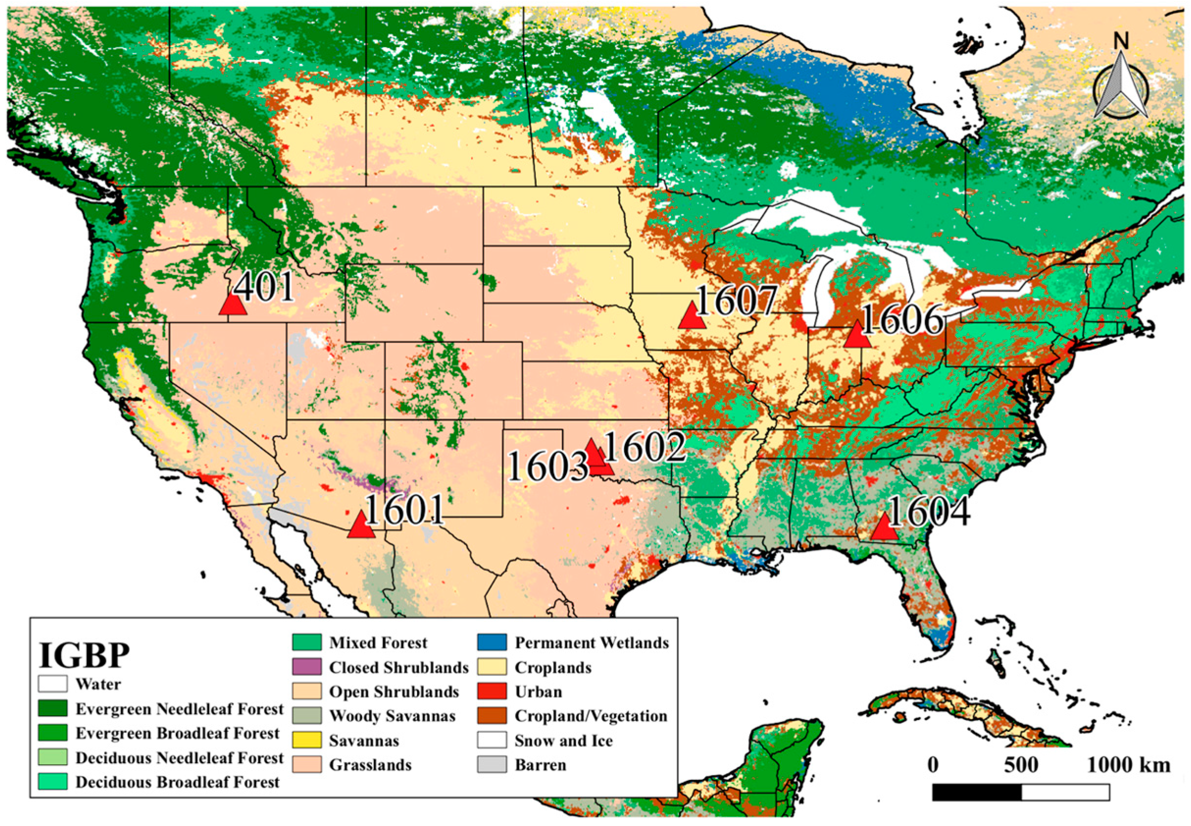
This study evaluates FT retrievals at SMAP core validation sites (CVS) located in CONUS. SMAP CVSs are densely sampled and usually consist of about ten stations covering a spatial extent of about 40 km by 40 km. Previous studies have used boreal (>45°N) latitude CVSs to validate the FT product [19,20]. Sites below 45°N have been used for soil moisture validation [21], but some of these sites should also be well-suited to assess SMAP FT retrievals at mid-latitudes.
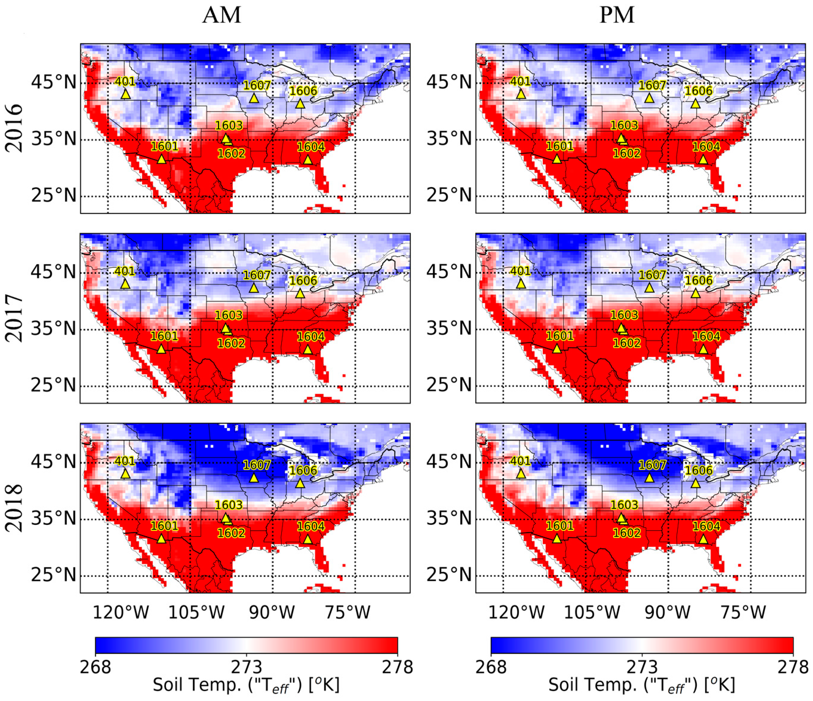
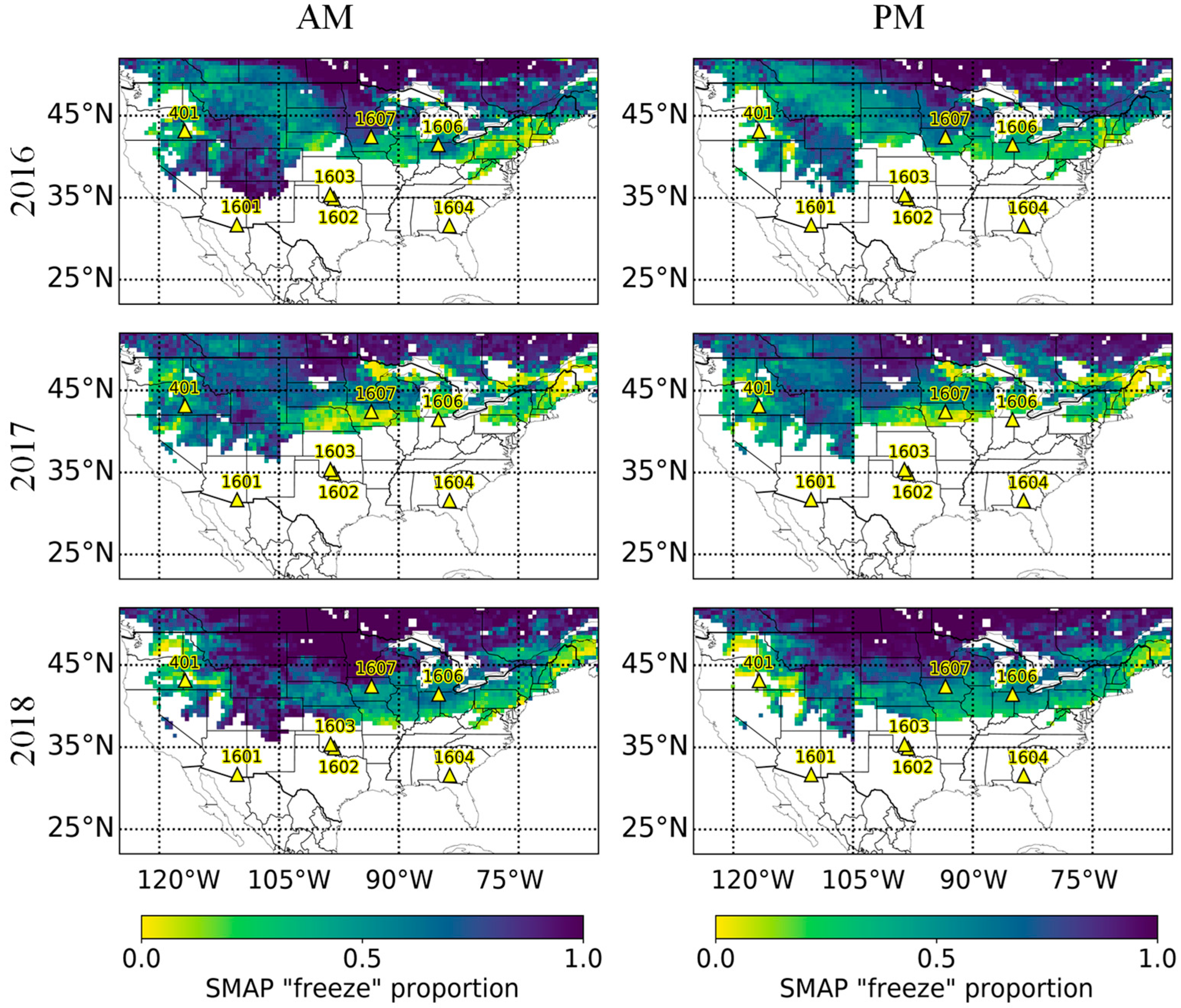
We use a detection approach similar to that used for the NASA SMAP FT product (L3_FT_P). Our hypothesis is that SMAP landscape FT retrievals would often (e.g., >70%) correspond to soil FT states at mid-latitude CVSs. This study is primarily concerned with evaluating SMAP retrievals against 0–5 cm soil temperature data collected at mid-latitude CVSs, but also maps annual (2016–2018) freeze extents in CONUS.

2. Data and Processing

2.1. SMAP Radiometer Data (L3_SM_P, Version 4)

The SMAP data record started on 31 March 2015 and provides global coverage every 2–3 days [3]. The radiometer has an ellipsoidal instantaneous field of view of 38 km by 49 km. SMAP observations are gridded on 362 km2 Equal Area Scalable Earth (EASE 2.0) grids for the standard product [22,23], but an enhanced product using 92 km2 grids is also available [24,25,26]. This study is limited to using the 362 km2 SMAP Level 3 Soil Moisture Passive (L3_SM_P, version 4) data [27].
L3_SM_P primarily provides volumetric soil moisture (m3/m3) data. This dataset also includes other gridded data, such as brightness temperature (Tb), which has been corrected for static water, and modeled soil temperature derived from the Goddard Earth Observing System Model Version 5 (GEOS-5) ‘Teff’ [28,29,30]. The L3_SM_P product includes up to two observations per grid per day. The observations correspond to local equator crossing times of 6 AM (descending orbit) and 6 PM (ascending orbit). This work used the L3_SM_P data as input to a seasonal threshold approach (STA) to produce a FT product (‘SMAP FT’) that extends below 45°N (Section 3.1).

2.2. Data Processing and Selection of Test Sites

Seasonal soil FT was examined at seven Agricultural Research Service (ARS) SMAP CVSs (Figure 1). SMAP CVSs are relatively densely sampled. Each site contains 15–54 stations located within about a 402 km2 region. The ARS network is the main network used for SMAP algorithm calibration and validation, and contains seven out of eight SMAP CVSs in CONUS [31].
SMAP retrieved landscape FT states are validated using 0–5 cm soil temperature data obtained from ARS. Hourly temperatures were examined for soil FT during the period of record (2001–present) at a total of 177 in situ stations. QA/QC checks were performed on the ARS data. First, soil temperatures colder than −20 °C and warmer than 50 °C were removed from the analysis. Then, the hourly soil temperatures at each station were also compared to the mean temperature of all stations at the SMAP CVS for that time-period; if that difference exceeded ±20 °C, those data were also removed. CVSs where soils seasonally froze were identified, and 6 AM/PM soil temperature data were compared to SMAP landscape FT retrievals (Table 1).
In situ data showed that soils only froze in Idaho, Iowa, and Indiana (Table 1). The coldest two months were either December and January or January and February. When averaged by month, soil temperatures fell below freezing only in Iowa (January and February). Iowa soils also froze most often, on average 75 days per year, followed by Indiana (40 days) and Idaho (31 days). Therefore, this study will be limited to the Idaho, Iowa, and Indiana CVSs.

2.3. Idaho, Iowa, and Indiana SMAP Grid Attributes

Idaho is located in a semi-arid climate and incorporates heterogeneous landscapes consisting of grasslands, hills, and some forested areas. The Indiana and Iowa CVSs are mostly homogeneous (croplands) and are located in a cold climate. At the Idaho, Iowa, and Indiana CVSs, stations are distributed over two, four, and one SMAP grids, respectively (Figure 2). The station centroid is located near the grid center in Indiana, but near the grid boundaries in Idaho and Iowa. Grids are labeled according to their indices in the SMAP grid geolocation data (https://nsidc.org/data/ease/tools).

3. Methods

3.1. FT Algorithm

The NASA SMAP FT algorithm uses a seasonal threshold approach (STA) to categorize radiometer retrievals as frozen or thawed. Compared to other FT delineation approaches, STA has the advantage of low data latency [4,33,34]. The first step of STA is to determine a seasonal scale factor Δ(t) based on a specific metric such as brightness temperature (Tb) or normalized polarization ratio (NPR) [4,19]. NPR is used to generate the NASA SMAP FT product and is defined as
NPR = ( Tb V Tb H ) / ( Tb V + Tb H )
in which TbV and TbH are the vertical and horizontal polarization, respectively.
In the NASA SMAP FT algorithm, freeze reference values (NPRfr) are found by averaging the 10 smallest NPR values occurring in January and February [19]. These months are selected because they are usually the coldest of the year in the northern hemisphere and have the greatest likelihood for landscape elements (i.e., soils) to be frozen. The same is done to compute thaw references (NPRth) but using the 10 largest NPR values occurring in July and August.
For each grid cell, date, and overpass (6 AM and 6 PM), the NPR(t) is computed and scaled by the upper (NPRth) and lower bounds (NPRfr), in which the seasonal scale factor Δ(t) is defined as
( t ) = ( NPR ( t ) NPR fr ) / ( NPR th NPR fr )
The seasonal scale factor is compared to threshold value Δ(t)thr to determine whether a landscape is frozen or thawed in which
if   ( t )   is   { > ( t ) thr ,   soil   state   is   thawed ( t ) thr , soil   state   is   frozen
In case of the standard NASA SMAP FT product (L3_FT_P), Δ(t)thr is equal to 0.5. If NPR(t) exceeds (falls below) the midpoint between the upper (NPRth) and lower bounds (NPRfr), the SMAP retrieval is set to thawed (frozen). The SMAP FT algorithm used in this study closely follows that of the NASA SMAP FT algorithm with few minor differences (Table 2). There are several reasons for the differences. The SMAP freeze-thaw (soil moisture) product has so far only been provided on the northern hemisphere (global) EASE grid. Since the goal of this work was to study a region not covered by the northern hemisphere EASE grid, data was instead taken from the soil moisture product. Also, the freeze-thaw signal at sub-boreal latitudes may not have a strong signature, and the STA is known to work better when the difference between NPRth and NPRfr is greater. Thus, only the smallest/largest 5 data were used to set the NPR references. The study wanted to only compare observational data that was collected at the same time; therefore, NPR(t) was set to ‘NA’ whenever a grid was not observed. To evaluate whether FT retrievals substantially changed depending on whether AM or PM data was used, AM and PM NPR thresholds were calculated separately and used to determine the FT state. Mitigation of FT retrieval errors was not attempted for the purpose of directly showing how well STA-based FT retrievals perform at the SMAP CVSs. A variable rather than constant Δ(t)thr was used to show how accuracy metrics vary with Δ(t)thr and to explore the extent to which FT retrieval accuracy could be optimized.

3.2. Classification Accuracy

Classification accuracy is evaluated following the approach in Derksen (2017) [19]. SMAP landscape FT retrievals and in situ soil observations are classified as either frozen or thawed. An error flag, ‘err’, is set based on comparisons of coincident observations (Equation (4))
err   is   { 0   if   SMAP = Obs 1   if   SMAP Obs
in which SMAP = 1 (0) if the SMAP retrieval is frozen (thawed) and Obs = 1 (0) if the in situ soil state corresponds to frozen (thawed). Furthermore, instances of ‘err’ = 1 were grouped into errors of omission (SMAP = 0, Obs = 1) and errors of commission (SMAP = 1, Obs = 0). Three accuracy metrics are used to summarize the results: ‘Freeze Accuracy’, ‘Thaw Accuracy’, and ‘Overall Accuracy’ (Equations (5)–(7)).
Freeze   Accuracy = 100     N SMAP = 1 , Obs = 1 / ( N total , Obs = 1 )
Thaw   Accuracy = 100     N SMAP = 0 , Obs = 0 / ( N total , Obs = 0 )
Overall   Accuracy = 100     ( N SMAP = 1 , Obs = 1 + N SMAP = 0 , Obs = 0 ) / ( N total )
in which N are counts of each of the combined SMAP and in situ states, Ntotal is the total number of events and Ntotal, and Obs=1 (Ntotal, Obs=0) are the total number of in situ frozen (thawed) occurrences. ‘Freeze Accuracy’ (‘Thaw Accuracy’) is the percentage of in situ frozen (thawed) states that SMAP identified correctly. ‘Overall Accuracy’ is the proportion of SMAP FT retrievals that correspond to the situ soil state.

3.3. Assessment of Factors That Impact SMAP Retrieval Accuracy

3.3.1. Data Aggregation Scheme

SMAP CVS stations are usually located within a 40 km radius but rarely fall within the same SMAP grid (Figure 2). There could be substantial landscape heterogeneity at this scale, and the impact of only using data collected at stations within a grid versus that of the entire CVS is not clear. Using data collected by a greater number of stations could reduce representativeness errors. The impact of in situ data aggregation method on SMAP soil FT accuracy metrics is investigated by aggregating in situ data by (1) grid and (2) centroid. The grid aggregation method averages temperature data of all stations within a SMAP grid. The centroid aggregation method averages data of all stations belonging to a CVS. SMAP data are taken from the grid cell containing the centroid of the stations that make up the CVS.

3.3.2. Temporal Subsets

NASA SMAP FT accuracy has been reported at variable time scales including the period of record of the active radar (April–July 2015) or a full year [19,20]. Derksen et al. (2017) reported that there are relatively more errors of commission during summer than winter [19]. Therefore, validation metrics were computed on annual basis and for a cold period, ‘winter’ (October through March).

3.3.3. NPR Threshold

A range of values for Δ(t)thr (from 0.01 through 2.00) were used to explore how validation metrics change as function of this threshold. Values greater than 1.00 are considered, because the NPR references (NPRfr, NPRth) do not necessarily include the global maximum or minimum value of NPR(t), because they are computed by averaging the five lowest (highest) values during January and February (July and August). The most extreme NPR(t) values may occur outside these periods.

3.3.4. Sampling Error

The validation of the SMAP retrieval algorithm is limited by the ability of in situ observations to accurately capture the FT state of the region encompassed by a SMAP grid. In situ stations are only able to sample a limited portion of the SMAP grid area, and stations are usually not well distributed throughout a grid. To estimate the impact of sampling on accuracy metrics, we relax the requirement that the average in situ temperatures are used. Instances in which SMAP retrievals and in situ data disagreed (SMAP = 0, Obs = 1 and SMAP = 1, Obs = 0) were re-evaluated to produce the ‘potential overall accuracy’ metric. This metric is calculated by counting SMAP retrievals as correct as long as at least one in situ station corroborated the SMAP retrieved soil state.

4. Results

4.1. Freeze and Thaw References Values

NPRfr is nearly identical irrespective of whether AM or PM observations are used (Table 3). However, NPRth(PM) is 10–20% greater than NPRth(AM) and explains the relatively greater dynamic range (ΔNPR) of PM observations. The dynamic range varies from 1.5 to 1.7, from 2.0 to 3.8, and from 3.6 to 4.5 for Idaho, Iowa, and Indiana, respectively, and is by far the lowest at the Idaho CVS.

4.2. SMAP FT Correspondence with In Situ Data

SMAP FT retrievals can be accurate during winter, especially when in situ soil temperatures clearly fall below 0 °C (Figure 3, Figure 4 and Figure 5). For Iowa and Indiana, SMAP FT retrievals were reasonably good, even when soil temperatures were close to freezing. In Idaho, SMAP FT retrievals only matched the in situ soil state when soil temperature fell below approximately −1 °C.
Because SMAP FT retrievals were not subject to error mitigation efforts, substantial errors of commission can be seen during summer (Figure 3, Figure 4 and Figure 5) when soils are quite warm. Figure 3 shows that Idaho has numerous non-winter frozen retrievals. The number of freeze retrievals (CVS averages) for 2015 to 2018 ‘summer’ data (April–September) are 174 (196), 74 (78), and 87 (60) for Idaho, Iowa, and Indiana AM (PM) observations, respectively.
In the conceptual framework of the SMAP FT algorithm, a lower (higher) NPR would generally correspond to lower (higher) temperature, because the soil state is frozen (thawed). Therefore, NPR(t) should be positively correlated with soil temperature. The winter temporal subset for Iowa shows good correlations of about 0.7 (0.75) for AM (PM) data (Figure 6). Idaho and Indiana have lower correlations of about 0.0 (−0.2) and 0.3 (0.4) for AM (PM) observations, respectively. Owing to errors of commission during summer, annual correlations between these quantities are poor (~0) or even negative (~−0.5 for Idaho). Therefore, neither the summer nor the annual temporal subsets should be used unless additional error mitigation steps are applied (e.g., the use of ancillary never frozen/thawed masks).
The distribution of observed temperatures by SMAP FT classification is shown in Figure 7. SMAP FT retrievals during winter accurately distinguish between cold and warm soils at the Iowa and Indiana CVSs. Results for AM (not shown) and PM data were similar. At these grids, the interquartile ranges (IQR) for frozen temperatures are small, and medians are located at or below 0 °C. Thawed temperatures vary greatly but are consistently warmer than 0 °C. SMAP FT retrievals clearly cannot distinguish between warm and cold soils at the Idaho CVS.

4.3. SMAP FT Retrieval Accuracy by Grid

SMAP winter accuracy varies by grid, CVS location, and performance metric, with overall accuracies usually greater than 70% for AM observations and modestly better for PM observations (75%) (Table 4). Improved PM validation metrics can probably be attributed to the greater ΔNPR as compared to AM values (Table 3). Accuracies for freeze are usually substantially smaller than those for thaw; thaw accuracies are rarely lower than 75%, while freeze accuracies were almost always less than 75%, regardless of locations. Because correct thaw classifications make up the major proportion (50–74%) of all classification results, and other categories (correct frozen detections, errors of commission, and errors of omission) range between 1% and 27%, the overall accuracy is highly influenced by thaw accuracy. Grid-to-grid variability within a CVS typically exceeded differences among CVSs. The northeastern Iowa grid (62892) had notably higher accuracies for all metrics.
CVS station averages compared to the SMAP centroid grid show that data aggregation can improve the accuracy metrics (Table 5). The overall accuracy improved by up to 5% for Idaho but did not change in Iowa. SMAP validation metrics in Idaho improved irrespective of whether the site was compared to the grid containing the centroid (60901) or the one below it (61865). Stations located in the southern grid (61865) had considerably warmer soil temperatures than in the northern grid. Thus, when all the Idaho stations were averaged, soil temperatures increased relative to the northern grid SMAP FT retrievals. This resulted in a decrease in the number of freeze events that were correctly classified and in an increase in the thaw events that were correctly classified. Similarly, soil temperatures decreases relative to the southern grid improved SMAP freeze accuracy but degraded the thaw accuracy.

4.4. Accuracy Metrics as Function of Δ(t)thr

The impact of the Δ(t)thr on validation metrics was analyzed using threshold values ranging from 0 to 2 (Figure 8). Clearly, the choice of seasonal scaling factor impacts the accuracy metrics. Figure 8 panels show that if Δ(t)thr is set equal to the smallest (largest) Δ(t), STA will classify all data as thawed (frozen). For example, results at grid 61865 show that high thaw (~99%) and overall (~95%) accuracy can be obtained if Δ(t) is set to zero (grid 61865, Figure 8).
Trivial cases can be avoided by selecting a Δ(t)thr in which both freeze accuracy and thaw accuracy are substantial (e.g., >50%). For most grids, nontrivial values for Δ(t)thr range from about 0.3 to 1.0. Additionally, it is important to maintain high overall accuracy. In most Figure 8 panels, overall accuracy has a global maximum somewhere between Δ(t)thr = 0.2 and Δ(t)thr = 0.8. When looking for a nontrivial solution, it can be useful to select a Δ(t)thr corresponding to points of inflection or local maxima.
Accuracy metrics can substantially increase when Δ(t)thr is changed by only a small amount from the NASA SMAP FT default value. For example, at grid 65806 AM, a Δ(t)thr ~ 0.4 could be selected to take advantage of the local maximum before the overall accuracy decreases. At this Δ(t)thr value, freeze, thaw, and overall accuracy are 70%, 87%, and 85%, respectively, compared to the default Δ(t)thr of 0.5, which gives a 72% accuracy for each metric.
Nontrivial values for Δ(t)thr ranged from about 0.2 to 1.0 at the CVS grids. Using Δ(t)thr = 0.5 would usually result in reasonably accurate, non-trivial values for each accuracy metric. Figure 8 clearly shows the trade-offs between accuracy metrics, as Δ(t)thr is varied. It is recommended to either use a default value of Δ(t)thr = 0.5 or to select a Δ(t)thr according to user needs (e.g., to maximize freeze accuracy, thaw accuracy, overall accuracy, or a combination of these).

4.5. Estimation of In Situ Sampling Error

Recognizing that there is considerable within-pixel variability of in situ temperatures, SMAP performance was re-examined using temperatures from individual stations (Figure 9). In many cases, when SMAP FT retrievals disagreed with in situ data, at least one station reported a temperature that agrees with the SMAP FT state. Station to station variability is greatest for Idaho and Indiana (usually close to ± 1 °C from the mean) but can also be substantial in Iowa (usually within ±0.5 °C from the mean). Most winter SMAP FT retrieval errors occur when soil temperatures are close to 0 °C.
Previous research has used a range of methods to account for variability and sampling errors of in situ observations. Here, the overall accuracy was recomputed in such a way that the SMAP FT detection was only flagged as erroneous if more than 75% of the stations in a grid had a soil state contrary to that determined by the SMAP algorithm (Table 6). Using this approach, SMAP FT retrieval accuracy values increased for all grids with 80% to 90% accuracy rates at most grids (Table 6).

4.6. CONUS FT Extent from L3_SM_P

There are some conceptual problems in transferring the NASA SMAP FT northern grid algorithm logic and applying it to CONUS. While it is reasonable to use July and August to compute NPRth (barring errors due to dense vegetation, and inundation), most soils in CONUS will not freeze during January and February. Setting of any NPRfr values where landscapes are thawed results in an incorrect calibration of the STA.
Therefore, this study uses a secondary dataset to limit SMAP FT retrievals to those areas where it is reasonable to define a seasonal freeze reference (NPRfr); the effective temperature ‘Teff’ [24], shown in Figure 10, is included in the SMAP L3_SM_P product and used to delimit freeze extents for CONUS (Figure 11). Regions where the average soil state was frozen were identified from January and February Teff values (≤273 K). Teff should be a reasonably good indicator of in situ FT states, because it is derived from the GEOS-5 model, which routinely assimilates soil temperature data at multiple depths from major national networks, including the ARS. According to Teff, natural soils at latitudes of about 35°N or higher froze in CONUS during the 2015 to 2018 period (Figure 10). Therefore, it is reasonable to define NPRfr values and to limit in situ comparisons to latitudes greater than about 35–40°N.
Maps of Teff (Figure 10) agree with the earlier finding (Table 1) that soils only froze in three of the CVSs (Idaho, Iowa, and Indiana) and that Teff is lower for Iowa than for the other CVSs.
PM data are usually about 1 K warmer than the AM data. Differences between the PM and AM maps can be used to identify transition regions where errors due to melt could potentially be mitigated by limiting analyses to SMAP AM data. However, the transition regions differ annually. Freeze extents were comparable between 2016 and 2017, but in 2018, the freeze extent extended about 1.5° latitude further south at locations east of 105°W. With respect to the SMAP CVSs, these maps show that Iowa froze each year, Indiana was above freezing in 2017, and Idaho had near-thawing temperatures in 2016 and 2018.
The annual temperature maps were used to delimit satellite-derived FT extents in CONUS to those regions where average Teff ≤ 273 K. Mean SMAP FT states for January and February were identified by the metric of SMAP ‘freeze fraction’. The freeze fraction was computed at each grid cell by dividing the number of SMAP freeze classifications by the total observations during January and February each year (Figure 11). SMAP freeze fraction maps are consistent with model temperature data (Figure 10). SMAP freeze retrieval rates were high (>0.5) in most regions that froze according to Teff. Both SMAP FT and Teff data show substantial spatial and interannual variability and also have similar patterns and trends. For example, in both sets of figures, 2018 was the coldest year and 2017 the warmest. In 2017, a relatively warm soil state extended eastward from about 105°W, while locations north of 45°N and west of 105°W were colder than in 2016.
SMAP FT maps did not agree with those for Teff in the Northeast and eastern Canada. In the Northeast, SMAP freeze rates are relatively lower (<0.5) than those for Canada east of 90°W (>0.5). Teff shows similar temperatures for both regions. One reason for this difference could be that the ΔNPR is very small over needleleaf forests (Figure 1 and Figure 12). Another possible explanation could be that because there are observational gaps in eastern Canada, GEOS-5 would more heavily rely on model results rather than in situ observations.
For most of CONUS, the PM dynamic range is greater than the AM dynamic range (Figure 12). This difference is especially pronounced in the Northern Great Plains region, where the PM dynamic range is greater by about 1 (or ~25% assuming NPRAM = 4). The CVS results indicated that FT states determined from PM overpass data are about 5% more accurate than from AM data (Table 4 and Table 5). This may be due to the larger PM dynamic range improving the STA [19].
Figure 12’s diurnal ΔNPR difference map (ΔNPRAM-ΔNPRPM) identifies regions where the AM dynamic range is greatest and those regions where the PM dynamic range is greatest. It can be used to select between the AM and PM observations, and shows that ΔNPRPM is greater than ΔNPRAM east of 105°W, whereas, ΔNPRAM is somewhat greater for a relatively small portion in the Northwest—a region that includes the Idaho CVS. However, this is not necessarily a strong indicator for the Idaho CVS, because the diurnal ΔNPR difference has considerable spatial variability near this CVS. In contrast, grids surrounding the Iowa and Indiana CVSs have much lower pixel-to-pixel variability, indicating that there is higher confidence in the PM observations. This result is supported by Table 4, which shows that PM observations were more accurate everywhere except at one Iowa grid (62892), where the overall accuracy remained about the same; however, PM observations could still be considered improved at this grid, because freeze accuracy improved by 7% while thaw accuracy only decreased by 3%.

5. Discussion

Derksen et al. (2017) found that the correlation between NPR time series with in situ temperature was improved for AM (~0.8) over PM (~0.3) observations. That study also found that SMAP PM FT data agreed better with in situ observations. This study found somewhat improved correlations for PM data in Iowa and Indiana: FT flag agreement improved about 5% when PM data was used. It is possible that PM validation metrics improved in part due to higher uncertainty in AM data caused by refreezing [19]. It is difficult to make a statement on error bias between AM and PM in this study, because commission or omission errors were similar (within 5%). Additionally, Derksen et al. (2017) limited their study to a thawing landscape, because it focused on the period during which the active radar collected data (April–July 2015) [19]. Our FT study focused on winter (October–March) but also included months during which landscape freeze-up and thaw occurred in CONUS.
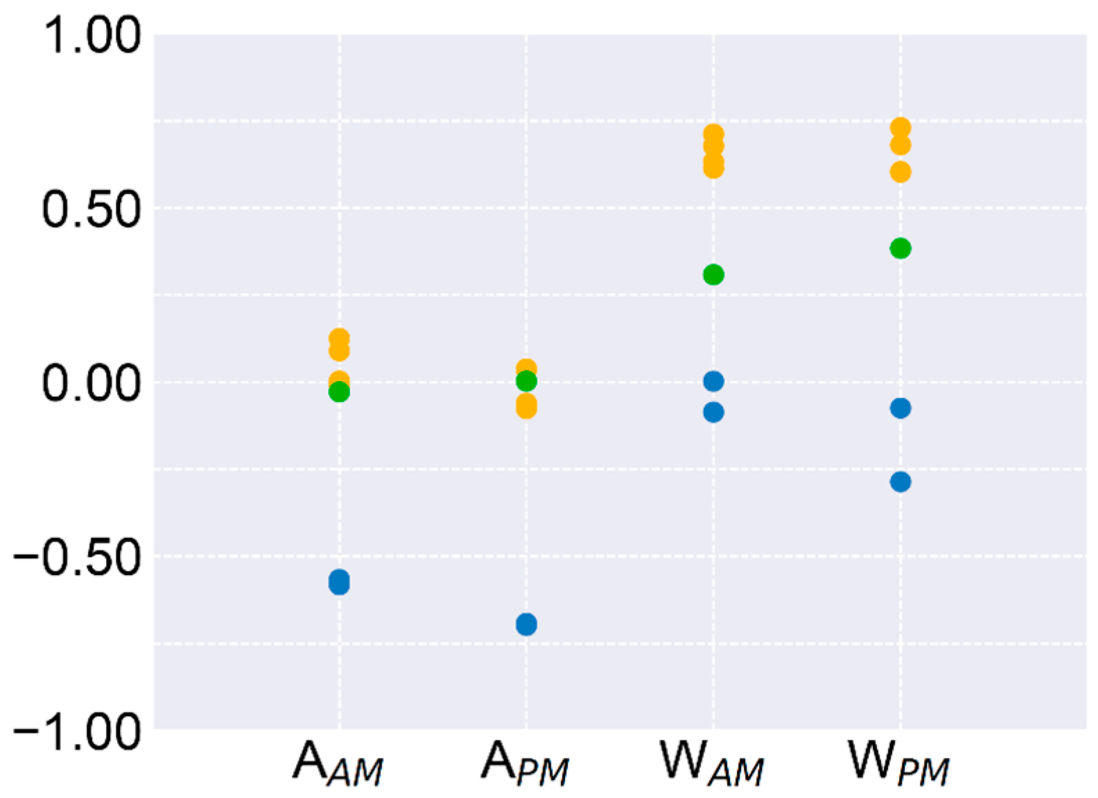
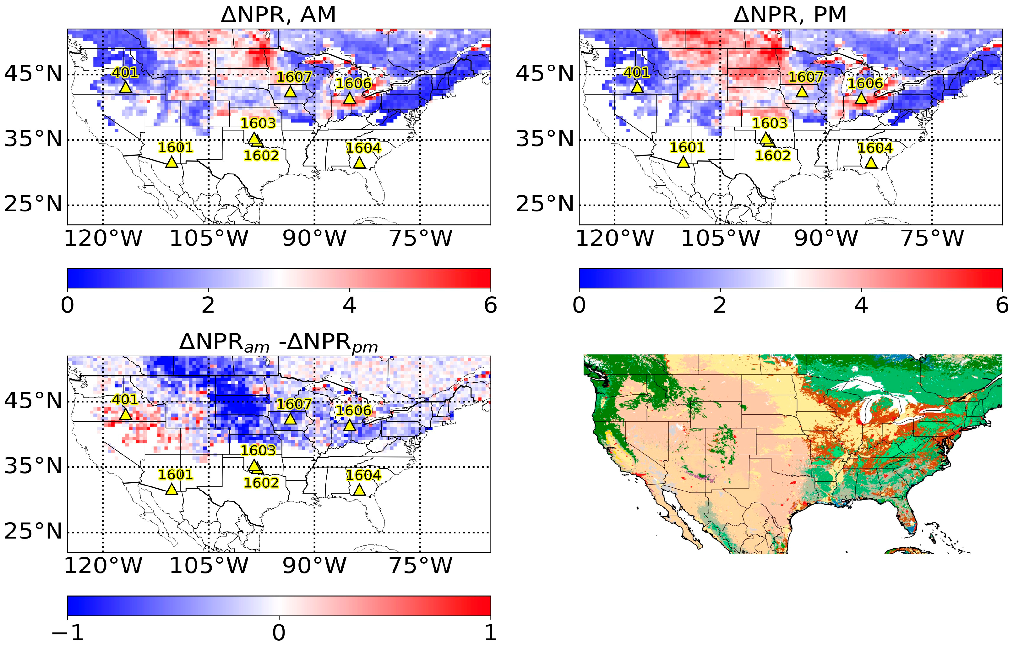
Although only a few sites were investigated, it was noted that validation metrics improved where greater ΔNPR values were found (Table 3 and Table 4). NPRfr was nearly constant between AM and PM overpasses, whereas NPRth was about 20% greater (Table 3, Figure 3, Figure 4 and 
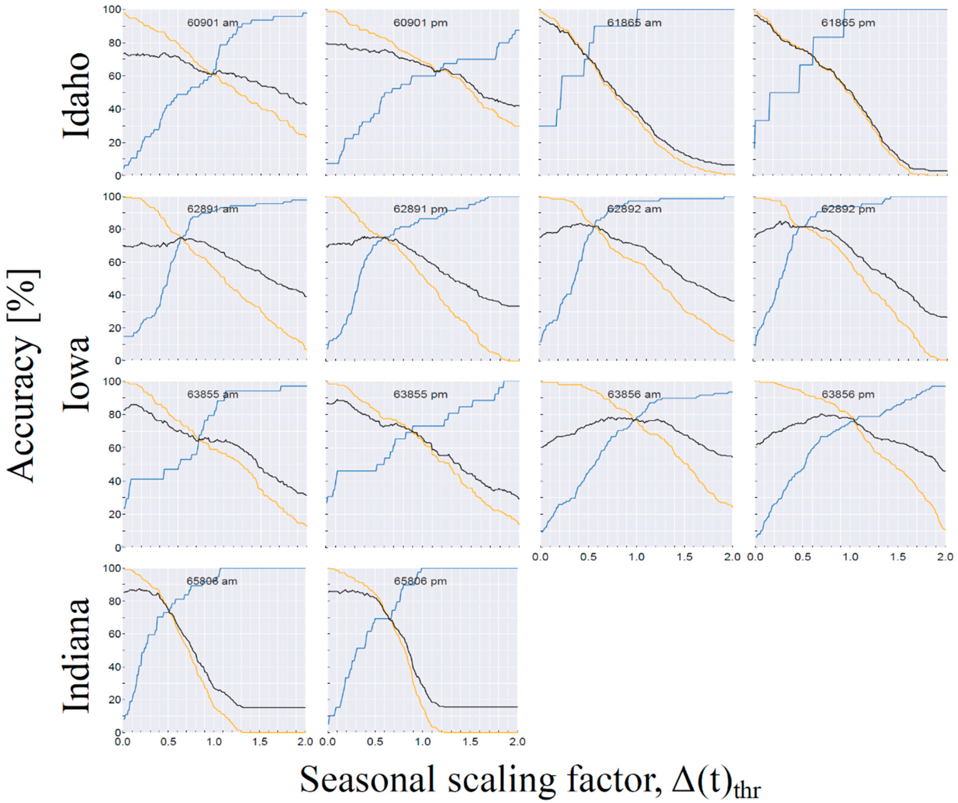
Figure 5). Overall accuracy for PM data was usually about 5% greater compared to AM. A likely explanation is that STA can, to a certain extent, more confidently delineate between freeze and thaw if greater ΔNPR values are used as input to the algorithm. Thus, the current approach for setting NPR references may produce a smaller than optimal ΔNPR range to be used in conjunction with STA, and accuracy metrics (for Δ(t)thr = 0.5) are not as good as they could be. It is also important to keep in mind that this work did not include any error mitigation efforts, and accuracy metrics may be improved further.
To follow up on the question as to why NPRth(PM) values could be 10–20% greater than NPRth(AM), a small case study was made for one Idaho grid (60901). Dates corresponding to the maximum five NPRth were 11 July 2015, 13 July 2015, 10 July 2016, 12 July 2016, and 14 August 2017 (11 July 2015, 14 July 2015, 11 July 2016, 27 July 2017, and 15 August 2017) for AM (PM) data. Dates obtained for AM and PM are nearly identical: Except for one “pair”, they are no more than one day apart from one another. The meteorological record at a weather station in Boise, ID (~50 km distance) indicated that there were only two precipitation events >1 mm in July/August 2015/2016, namely, on 10 July 2015 between 8 AM—4 PM (about 8 mm) and on 10 July 2016 between noon and 6 PM (about 15 mm). It follows that if it is true that summer convective precipitation would provide more water to soils during a 6 AM to 6 PM window vs. a 6 PM to 6 AM window, then it should be expected that NPRth(PM) would be somewhat increased for 6 PM observations relative to those made at 6 AM—and explain the increase in NPRth(PM).
An important limitation of methodology is that SMAP FT detection relies on a method traditionally used to estimate water content in landscape elements (vegetation, and soils). NPR is equivalent to the Microwave Polarization Difference Index (MPDI), which is a well-established quantity that has been used to characterize whether a landscape (e.g., soil, vegetation) is wet or dry [35,36]. Liquid water, dry soil, and ice, respectively, have dielectric constants (εr) of approximately 80, 5, and 3 [3,37]. Therefore, frozen soil—irrespective of its frozen water content—would have a dielectric constant that is comparable to that of dry soil. Thus, SMAP classification results should then also be interpreted as ‘wet’ (thawed) and ‘dry’ (frozen).
The higher incidence of SMAP ‘frozen’ retrievals during summer (Figure 4) can be attributed to Idaho being relatively drier than the other CVS (semi-arid, Table 1). For dry sites such as the Idaho CVS, it would be valuable to develop and test alternative FT retrieval methods that do not depend on NPR, such as the one presented in Kim et al. (2011) [4]. That method also used the STA approach, but applied it to TbV rather than NPR. L3_FT_P version 2 uses the TbV-based type of FT retrieval at most grids below 45°N [38].
Accuracy assessment of SMAP landscape FT retrievals is difficult due to the impact of landscape heterogeneity on coarse resolution observations. The SMAP radiometer has an ellipsoidal instantaneous field of view of 38 by 49 km and therefore incorporates landscape elements that are not accounted for with station point data. At the studied CVSs, there are geographic biases in the siting of stations with respect to each SMAP grid: Stations in grids 60901 (Idaho), 62891 (Iowa), 62892 (Iowa), and 65806 (Indiana) are located inside a radius of about 20 km. Stations in grids 68165, 63855, and 63856 are located inside a radius of 10 km or less, and they cover less of the SMAP grid area.
The best accuracy metrics between SMAP FT and in situ temperature data were obtained in Iowa (grid 62891) and Indiana (grid 65806). Relatively poorer results in Idaho may be attributed to the small ΔNPR and the semi-arid climate. The semi-arid climate factors into a higher rate of errors of commission, because NPR/MPDI discriminates between dry/wet rather than freeze/thaw.
Idaho also features a heterogeneous landscape that is better represented by in situ data if all station data are used, rather than dividing station data according to grids (Section 4.3). Compared to the boreal study, ΔNPR at grasslands and croplands situated in CONUS were substantially smaller. In the boreal study, ΔNPR averaged about 2.9 (3.9) for grassland (cropland) compared to our results of 1.5 (2.6). While lower, ΔNPR obtained at CONUS CVSs are within one standard deviation of those obtained in the boreal NASA SMAP FT study. Even at fairly homogenous CVSs (Iowa and Indiana), significant sub-grid variability exists (Figure 9).
The relatively greater ΔNPR obtained in the boreal study for grasslands and croplands could potentially be attributed to NPRfr values in that region that are more representative of fully frozen soils than the current study. Reliable NPRfr values need soils within a landscape (SMAP grid) to be frozen to a greater depth than the L-band penetration depth—a condition that is more difficult to satisfy at lower latitudes. However, data obtained in the boreal study for the Canadian Prairie region (grasslands and croplands) do not support this idea: The prairie NPRfr values (~3) exceeded those at SMAP CVSs (2.4). However, prairie NPRth values were much larger (>6) than those obtained at SMAP CVSs (~5). The boreal study’s ΔNPR map indicates that the Canadian Prairie region typically has ΔNPR values between 3 and 4, a similar range to the mean values that were reported for their study’s grasslands (2.9) and croplands (3.9). Thus, the relatively smaller ΔNPR for CONUS grassland and cropland sites could more likely be attributed to their relatively smaller NPRth. While the Canadian Prairie region is dry, the region’s climatology indicates that much of their annual rainfall totals occurs during a July/August window, with July/August totals decreasing with decreasing latitude [39]. If the 2015 July/August precipitation totals followed a similar spatial pattern, then this could explain why the July/August NPRth values were greater in the boreal study than for CONUS. However, this perspective is limited to only looking at the Canadian Prairies and a few locations in CONUS. Further exploration is needed to conclusively support the above conjecture regarding greater NPRth and ΔNPR mean values for grasslands and croplands in the boreal study compared to at CONUS CVSs.
Another important aspect is that landscape heterogeneity can also be caused by ephemeral water (EW). Because FT algorithms exploit the substantial dielectric constant differences as water transitions from frozen to liquid (and vice versa), it is important to be aware that the SMAP observations would be additionally impacted by EW on land. While SMAP Tb values are routinely corrected for static water [30], EW is a potential source of error. For example, wet snow may result in a ‘thawed’ SMAP FT retrieval, while the soil may still be frozen [19]. In this case, the soil state cannot be directly detected, because a surficial water layer or wet snow masks the soil’s emission. Spring and midwinter thawing may also produce ephemerally flooded areas within a landscape. Due to its high sensitivity to liquid water, even a localized event can significantly impact the SMAP FT retrieval accuracy within its footprint. However, dry snow can also be a source of error in FT retrievals at L-band because of refraction and impedance matching [40,41]. These effects impact Tb such that the Tb signal more closely corresponds to that of a frozen soil: The NPR of frozen soil covered by dry snow would be lower than that of bare frozen soil. Thus, it is possible to have a false frozen retrieval in the case of a wet soil being covered by dry snow. This situation is possible early in the cold season. If snowpack properties and moisture at the snow/soil interface were available, we could study this potential source of error in more detail.
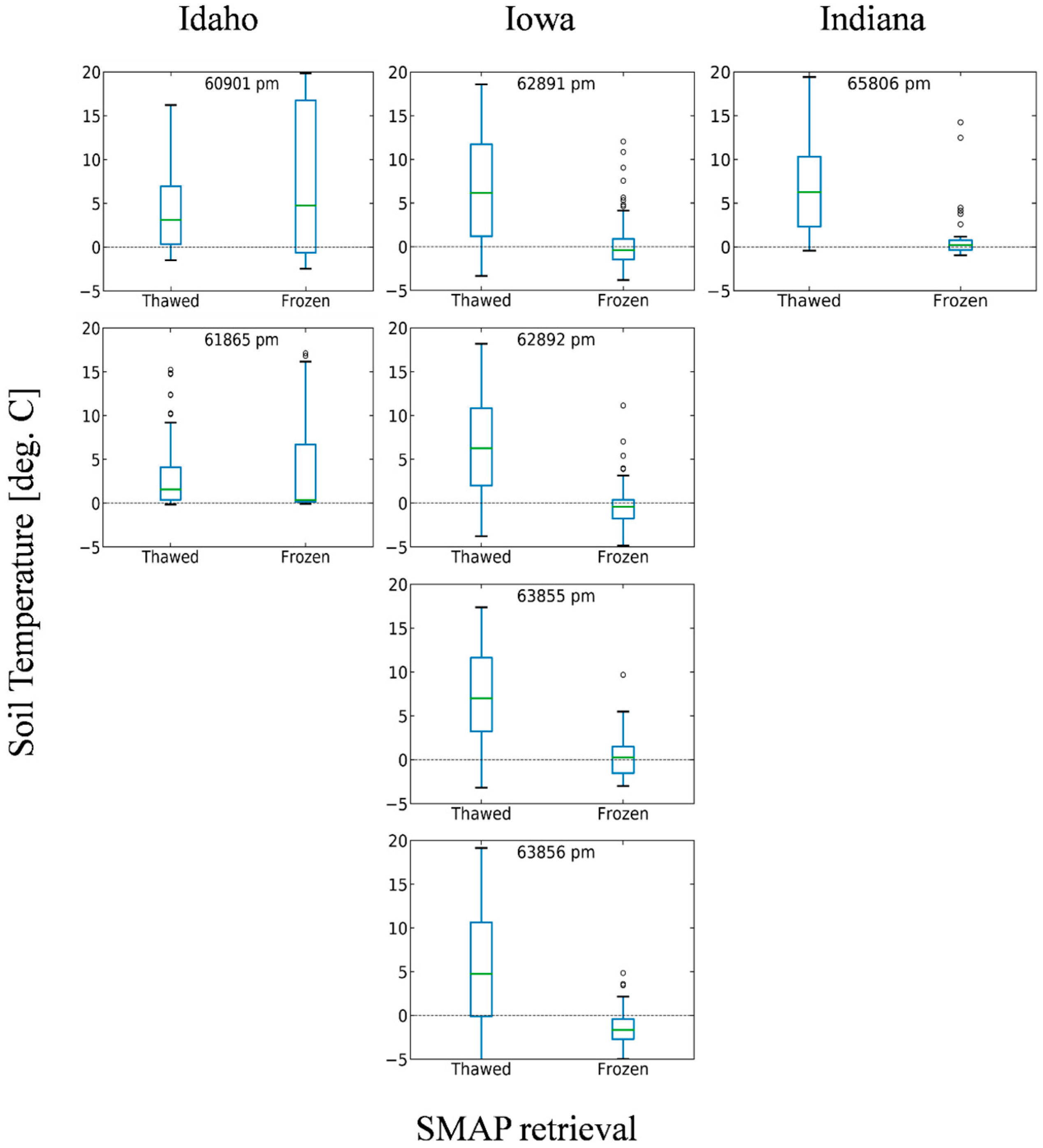
Limiting assumptions related to FT to binary classification can also impact accuracy assessment, mainly because relatively small differences in temperature change the classification of soil FT. Small measurement uncertainty or instrumentation bias could lead to errors in observed soil state. Thermistors used at the CVSs are optimally calibrated for a temperature of 20 °C and would have errors ranging from ±0.1–0.3 °C at near-freezing temperatures. In situ FT detections might be more robust if the soil dielectric constant were used instead of soil temperature. Also, the temperature at which natural soils freeze is usually lower than 0 °C, and a significant portion of water may remain in a liquid phase until soil temperatures fall well below freezing (e.g., −0.5 °C). Freezing point depression would impact SMAP FT validation accuracy metrics, because soil may still be wet/thawed when its physical temperature is less than 0 °C. During thaw, soils often become isothermal for an extended period of time. In this state, both ice and water are present, and it is reasonable to refer to this state as either frozen or thawed.
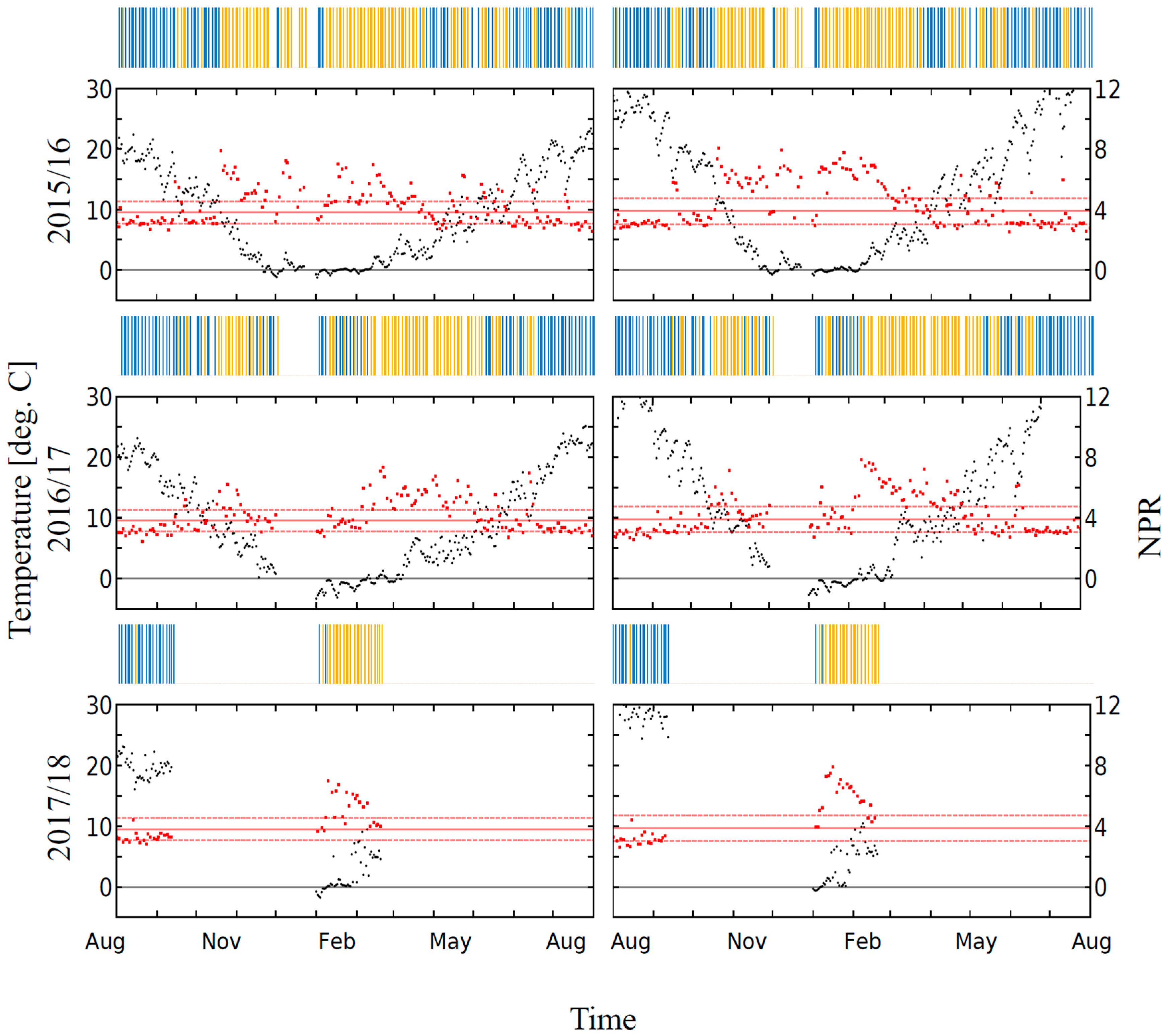
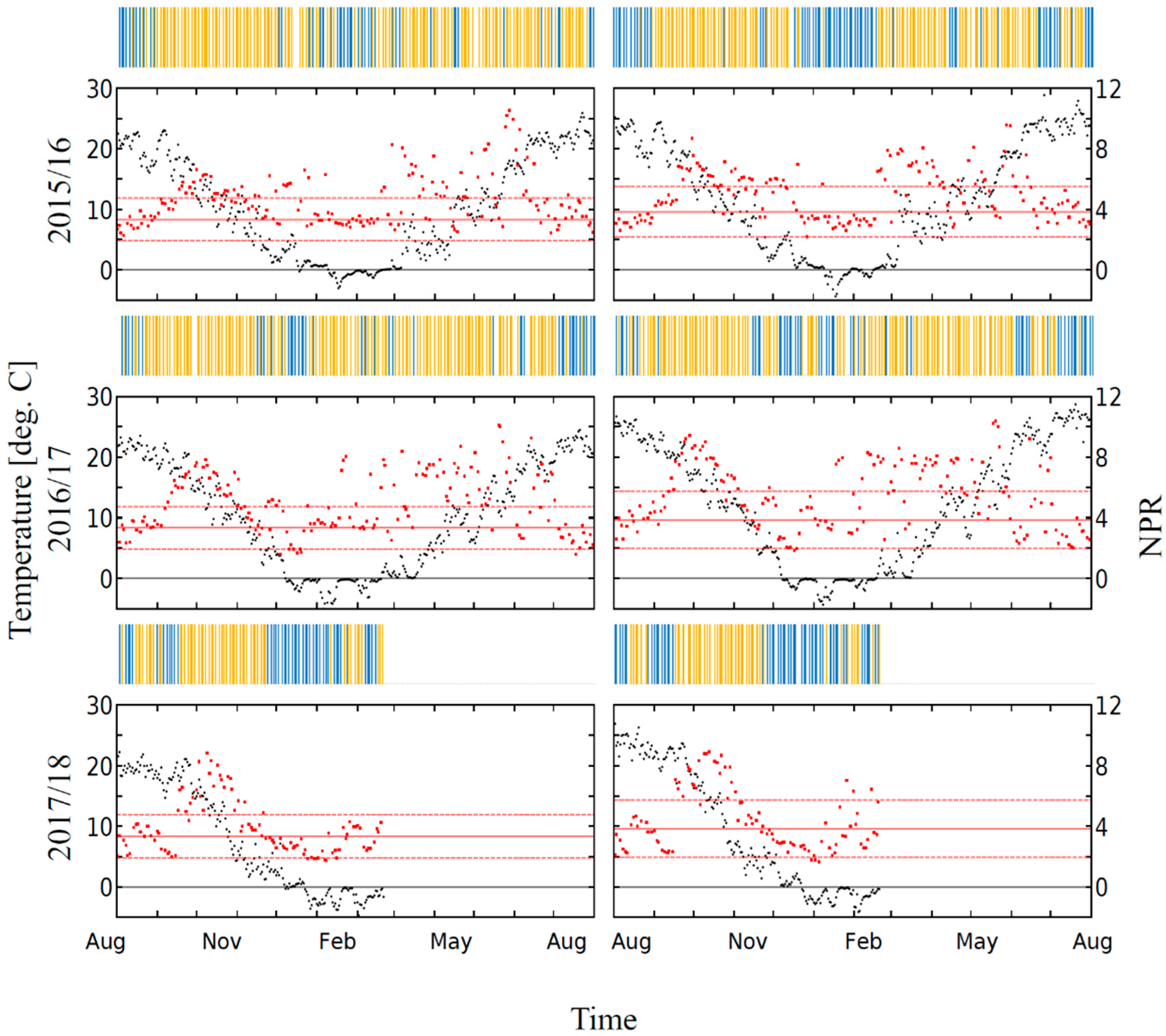
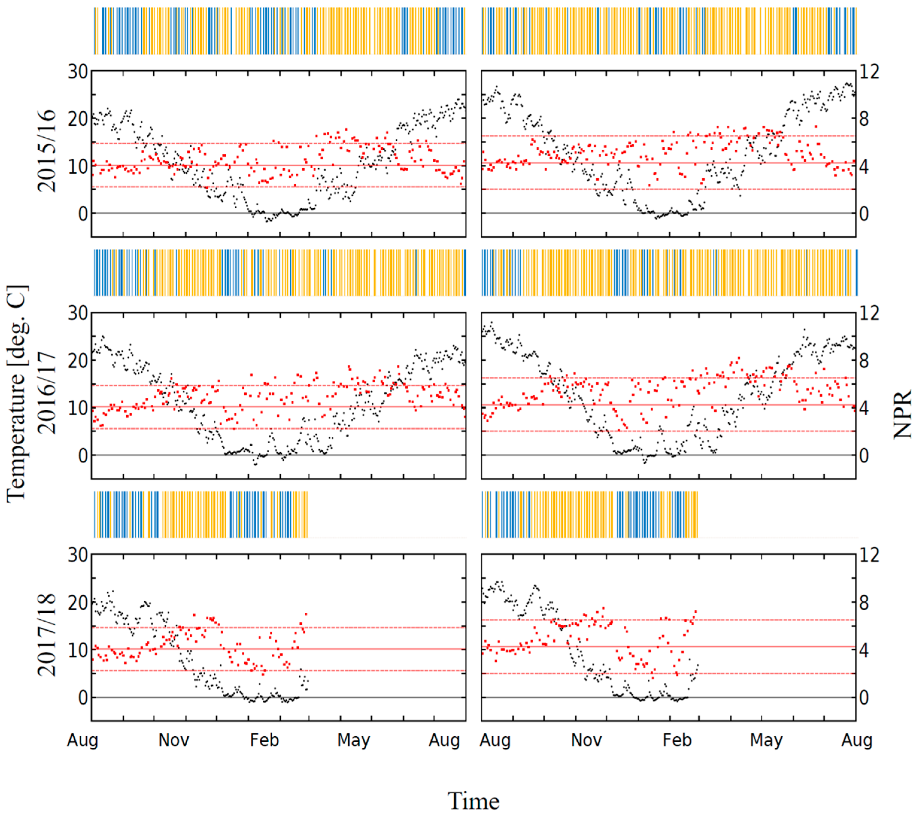
It is possible to improve on the shortcomings of binary classification by aggregating in situ soil temperature data according to SMAP FT retrieval. In this representation, if SMAP retrievals are sensible, frozen soils would be colder and show median temperatures close to or below freezing. Figure 7 showed that SMAP landscape FT retrievals corresponded quite well with soil temperatures at most grids, indicating that there should be good confidence in SMAP FT retrievals of the landscape state corresponding to soil temperature at least at some locations in CONUS.
A priori knowledge of where SMAP FT retrievals are accurate would be especially valuable for sub-boreal latitudes, because it is important to only define freezing thresholds where landscape elements (i.e., soils) freeze. Inappropriate application of thresholds will cause the interpretation of results to be extremely difficult, because classification results are impacted by retrievals over forested areas or in climates that are both dry and cold. Version 2 of L3_FT_P addresses this issue by only using the STA at those locations where model data indicated frozen conditions for at least 20 days per year. This work also identified some indicators leading to improved SMAP FT retrievals. Here, the optimal frozen condition appears to be greater than 20 days. The best performance was obtained in the Iowa CVS. Iowa had nearly twice the frozen duration per year (75 days) and colder soil temperatures that were considerably colder than Idaho or Indiana. The temperature of frozen soils should also be considered. SMAP landscape FT retrievals would probably be more accurate if soils froze longer and colder (e.g., average temperature below <−1.0 °C). Finally, the STA is not recommended for locations where ΔNPR < 2.

6. Summary and Conclusions

This work compared spaceborne L-band microwave-based landscape freeze-thaw retrievals from the SMAP radiometer to soil temperatures at SMAP core validation sites consisting of seven SMAP grids located at latitudes between 41–43°N in the contiguous United States. This work tested SMAP FT retrievals using a seasonal threshold algorithm applied to SMAP soil moisture data (L3_SM_P) to produce a FT product (‘SMAP FT’) that extends south of 45°N.
Results showed that FT retrievals with overall accuracy greater than 70% can be obtained using a seasonal threshold approach (STA) when analysis is restricted to October to March. This is because there were many errors of commission during April to September. Overall accuracy usually exceeded 70% (75%) for AM (PM) at all CVSs. SMAP FT corresponded best with Iowa and Indiana in situ temperatures. Correlations were the highest in Iowa (0.7), followed by Indiana (0.3) and Idaho (0.0). SMAP FT retrievals were also found to be accurate at distinguishing between cold and warm soils except in Idaho. SMAP accuracy metrics may be better for PM than AM overpass data simply due to a greater dynamic range for the normalized polarization ratio (NPR). A map of the diurnal difference in the dynamic range of NPR indicated that PM retrievals are preferable for most of CONUS. SMAP accuracy metrics are also sensitive to the choice of the seasonal scale factor and, potentially, the data aggregation scheme. As to sub-grid heterogeneity, usually one or more CVS stations agreed with SMAP FT, even when the station average did not. If SMAP FT retrievals are only counted as error when 75% of the stations indicated a contrary soil state, retrieval accuracy could be as high as 80% to 90% at most grids. Annual maps of January and February freeze rates show that there are significant interannual and spatial differences in the frequency with which each grid froze.
While SMAP landscape FT retrievals show good correspondence with in situ soil temperatures in CONUS, further work is needed to assess SMAP FT quality for mid-latitudes. Accurate SMAP soil state retrievals are more challenging at sub-boreal latitudes due to higher occurrence of midwinter thawing, and more persistent and denser vegetation. SMAP FT retrievals are challenging in cold semi-arid landscapes, due to their tendency to have soils dry enough to cause errors of commission.

Author Contributions

S.K. and J.M.J. designed the study. S.K. obtained and processed the datasets with support of M.C., M.S., J.P., and S.L., S.K. and J.M.J. analyzed and interpreted the results with support of R.S. and E.C., S.K. wrote the manuscript with support of J.M.J., R.S., and E.C.

Acknowledgments

This work was supported by NASA Research Opportunities in Earth and Space Sciences (ROSES), NNX16AN34G.

Conflicts of Interest

The authors declare no conflict of interest. The founding sponsors had no role in the design of the study; in the collection, analyses, or interpretation of data; in the writing of the manuscript; or in the decision to publish the results.

References

  1. Zhang, T. Investigation of the near-surface soil freeze-thaw cycle in the contiguous United States: Algorithm development and validation. J. Geophys. Res. 2003, 108, 8860. [Google Scholar] [CrossRef]
  2. Colliander, A.; McDonald, K.; Zimmermann, R.; Schroeder, R.; Kimball, J.S.; Njoku, E.G. Application of quikSCAT backscatter to SMAP validation planning: Freeze/Thaw state over ALECTRA sites in Alaska from 2000 to 2007. IEEE Trans. Geosci. Remote Sens. 2012, 50, 461–468. [Google Scholar] [CrossRef]
  3. Entekhabi, D.; Yueh, S.; O’Neill, P.E.; Kellogg, K.H.; Allen, A.; Bindlish, R.; Brown, M.; Chan, S.; Colliander, A.; Crow, W.T. SMAP Handbook; JPL: Pasadena, CA, USA, 2014.
  4. Kim, Y.; Kimball, J.S.; Mcdonald, K.C.; Member, S.; Glassy, J. Developing a Global Data Record of Daily Landscape Freeze/Thaw Status Using Satellite Passive Microwave Remote Sensing. IEEE Trans. Geosci. Remote Sens. 2011, 49, 949–960. [Google Scholar] [CrossRef]
  5. Kimball, J.S.; McDonald, K.C.; Frolking, S.; Running, S.W. Radar remote sensing of the spring thaw transition across a boreal landscape. Remote Sens. Environ. 2004, 89, 163–175. [Google Scholar] [CrossRef]
  6. Zwieback, S.; Paulik, C.; Wagner, W. Frozen soil detection based on advanced scatterometer observations and air temperature data as part of soil moisture retrieval. Remote Sens. 2015, 7, 3206–3231. [Google Scholar] [CrossRef]
  7. Du, J.; Kimball, J.S.; Azarderakhsh, M.; Dunbar, R.S.; Moghaddam, M.; McDonald, K.C. Classification of Alaska spring thaw characteristics using satellite L-band radar remote sensing. IEEE Trans. Geosci. Remote Sens. 2015, 53, 542–556. [Google Scholar]
  8. Pastick, N.J.; Jorgenson, M.T.; Wylie, B.K.; Nield, S.J.; Johnson, K.D.; Finley, A.O. Distribution of near-surface permafrost in Alaska: Estimates of present and future conditions. Remote Sens. Environ. 2015, 168, 301–315. [Google Scholar] [CrossRef] [Green Version]
  9. Cherkauer, K.A.; Lettenmaier, D.P. Hydrologic effects of frozen soils in the upper Mississippi River basin. J. Geophys. Res. Atmos. 1999, 104, 19599–19610. [Google Scholar] [CrossRef] [Green Version]
  10. Campbell, J.L.; Ollinger, S.V.; Flerchinger, G.N.; Wicklein, H.; Hayhoe, K.; Bailey, A.S. Past and projected future changes in snowpack and soil frost at the Hubbard Brook Experimental Forest, New Hampshire, USA. Hydrol. Process. 2010, 24, 2465–2480. [Google Scholar] [CrossRef]
  11. Ovik, J.M.; Siekmeier, J.A.; Van Deusen, D.A. Improved Spring Load Restriction Guidelines Using Mechanistic Analysis; Minnesota DOT Report No. 2000-18; Minnesota Department of Transportation: Saint Paul, MN, USA, 2000.
  12. Judge, J.; Member, S.; Galantowicz, J.F.; England, A.W.; Dahl, P. Freeze/Thaw Classification for Prairie Soils Using SSM/I Radiobrightnesses. IEEE Trans. Geosci. Remote Sens. 1997, 35, 827–832. [Google Scholar] [CrossRef]
  13. Rautiainen, K.; Lemmetyinen, J.; Pulliainen, J.; Vehvilainen, J.; Drusch, M.; Kontu, A.; Kainulainen, J.; Seppänen, J. L-band radiometer observations of soil processes in boreal and subarctic environments. IEEE Trans. Geosci. Remote Sens. 2012, 50, 1483–1497. [Google Scholar] [CrossRef]
  14. Kalantari, P.; Bernier, M.; McDonald, K.C.; Poulin, J. Using available time series of Passive and Active Microwave to develop SMAP Freeze/Thaw algorithms adapted for the canadian subarctic. In Proceedings of the 2014 IEEE International Geoscience and Remote Sensing Symposium (IGARSS), Quebec City, QC, Canada, 13–18 July 2014; pp. 2550–2553. [Google Scholar]
  15. Roy, A.; Royer, A.; Derksen, C.; Brucker, L.; Langlois, A.; Mialon, A.; Kerr, Y.H. Evaluation of spaceborne L-band radiometer measurements for terrestrial freeze/thaw retrievals in Canada. IEEE J. Sel. Top. Appl. Earth Obs. Remote Sens. 2015, 8, 4442–4459. [Google Scholar] [CrossRef]
  16. Rautiainen, K.; Lemmetyinen, J.; Schwank, M.; Kontu, A.; Ménard, C.B.; Mätzler, C.; Drusch, M.; Wiesmann, A.; Ikonen, J.; Pulliainen, J. Detection of soil freezing from L-band passive microwave observations. Remote Sens. Environ. 2014, 147, 206–218. [Google Scholar] [CrossRef]
  17. Rautiainen, K.; Parkkinen, T.; Lemmetyinen, J.; Schwank, M.; Wiesmann, A.; Ikonen, J.; Derksen, C.; Davydov, S.; Davydova, A.; Boike, J. SMOS prototype algorithm for detecting autumn soil freezing. Remote Sens. Environ. 2016, 180, 346–360. [Google Scholar] [CrossRef]
  18. Kim, Y.; Kimball, J.S.; Glassy, J.; Du, J. An extended global Earth system data record on daily landscape freeze–thaw status determined from satellite passive microwave remote sensing. Earth Syst. Sci. Data 2017, 9, 133–147. [Google Scholar] [CrossRef] [Green Version]
  19. Derksen, C.; Xu, X.; Scott Dunbar, R.; Colliander, A.; Kim, Y.; Kimball, J.S.; Black, T.A.; Euskirchen, E.; Langlois, A.; Loranty, M.M.; et al. Retrieving landscape freeze/thaw state from Soil Moisture Active Passive (SMAP) radar and radiometer measurements. Remote Sens. Environ. 2017, 194, 48–62. [Google Scholar] [CrossRef]
  20. Li, X.; McColl, K.A.; Lyu, H.; Xu, X.; Derksen, C.; Lu, H.; Entekhabi, D. Validation of the SMAP freeze/thaw product using categorical triple collocation. Int. Geosci. Remote Sens. Symp. 2017, 205, 1596–1598. [Google Scholar] [CrossRef]
  21. Jackson, T.; Colliander, A.; Kimball, J.; Reichle, R.; Crow, W.; Entekhabi, D.; O’Neill, P.; Njoku, E. SMAP Science Data Calibration and Validation Plan; JPL D-52544; JPL: Pasadena, CA, USA, 2012.
  22. Brodzik, M.J.; Billingsley, B.; Haran, T.; Raup, B.; Savoie, M.H. EASE-Grid 2.0: Incremental but Significant Improvements for Earth-Gridded Data Sets. ISPRS Int. J. Geo-Inf. 2012, 1, 32–45. [Google Scholar] [CrossRef] [Green Version]
  23. Brodzik, M.; Billingsley, B.; Haran, T.; Raup, B.; Savoie, M. Correction: EASE-Grid 2.0: Incremental but Significant Improvements for Earth-Gridded Data Sets. ISPRS Int. J. Geo-Inf. 2014, 3, 1154–1156. [Google Scholar] [CrossRef]
  24. Chan, S.; Bindlish, R.; O’Neill, P.; Jackson, T.; Chaubell, J.; Piepmeier, J.; Dunbar, S.; Colliander, A.; Chen, F.; Entekhabi, D.; et al. Development and validation of the SMAP enhanced passive soil moisture product. In Proceedings of the 2017 IEEE International Geoscience and Remote Sensing Symposium (IGARSS), Fort Worth, TX, USA, 23–28 July 2017; pp. 2539–2542. [Google Scholar] [CrossRef]
  25. Chan, S.K.; Bindlish, R.; O’Neill, P.; Jackson, T.; Njoku, E.; Dunbar, S.; Chaubell, J.; Piepmeier, J.; Yueh, S.; Entekhabi, D. Development and assessment of the SMAP enhanced passive soil moisture product. Remote Sens. Environ. 2018, 204, 931–941. [Google Scholar] [CrossRef]
  26. Colliander, A.; Jackson, T.J.; Chan, S.K.; O’Neill, P.; Bindlish, R.; Cosh, M.H.; Caldwell, T.; Walker, J.P.; Berg, A.; McNairn, H.; et al. An assessment of the differences between spatial resolution and grid size for the SMAP enhanced soil moisture product over homogeneous sites. Remote Sens. Environ. 2018, 207, 65–70. [Google Scholar] [CrossRef]
  27. O’Neill, P.E.; Chan, S.; Njoku, E.G.; Jackson, T.; Bindlish, R. SMAP L3 Radiometer Global Daily 36 km EASE-Grid Soil Moisture, Version 4. Available online: http://nsidc.org/data/SPL3SMP (accessed on 1 January 2018).
  28. Chan, S.K.; Bindlish, R.; O’Neill, P.E.; Njoku, E.; Jackson, T.; Colliander, A.; Chen, F.; Burgin, M.; Dunbar, S.; Piepmeier, J.; et al. Assessment of the SMAP Passive Soil Moisture Product. IEEE Trans. Geosci. Remote Sens. 2016, 54, 4994–5007. [Google Scholar] [CrossRef]
  29. SMAP Algorithm Development Team. SMAP Sience Team SMAP Ancillary Data Report on Surface Temperature. Available online: http://smap.jpl.nasa.gov/system/internal_ resources/details/original/293_051_surf_temp_150304.pdf (accessed on 4 January 2018).
  30. Chan, S. SMAP Ancillary Data Report on Static Water Fraction; Jet Propuls. Lab., Calif. Inst. Technol.: Pasadena, CA, USA, 2013.
  31. Colliander, A.; Jackson, T.J.; Bindlish, R.; Chan, S.; Das, N.; Kim, S.B.; Cosh, M.H.; Dunbar, R.S.; Dang, L.; Pashaian, L.; et al. Validation of SMAP surface soil moisture products with core validation sites. Remote Sens. Environ. 2017, 191, 215–231. [Google Scholar] [CrossRef]
  32. Peel, M.C.; Finlayson, B.L.; McMahon, T.A. Updated world map of the Köppen-Geiger climate classification. Hydrol. Earth Syst. Sci. Discuss. 2007, 4, 439–473. [Google Scholar] [CrossRef]
  33. Dunbar, S.; Xu, X.; Colliander, A.; Derksen, C.; Kimball, J.; Kim, Y. SMAP Level 3 Radiometer Freeze/Thaw Data Products. Available online: https://nsidc.org/sites/nsidc.org/files/technical-references/L3_FT_P_ATBD_v7.pdf (accessed on 12 January 2018).
  34. Xu, X.; Dunbar, S.; Derksen, C.; Colliander, A.; Kim, Y.; Kimball, J.S. SMAP L3 Radiometer Northern Hemisphere Daily 36 km EASE-Grid Freeze/Thaw State, Version 1. Available online: http://nsidc.org/data/SPL3FTP (accessed on 4 January 2018).
  35. Schroeder, R.; McDonald, K.C.; Chapman, B.D.; Jensen, K.; Podest, E.; Tessler, Z.D.; Bohn, T.J.; Zimmermann, R. Development and evaluation of a multi-year fractional surface water data set derived from active/passive microwave remote sensing data. Remote Sens. 2015, 7, 16688–16732. [Google Scholar] [CrossRef]
  36. Owe, M.; de Jeu, R.; Walker, J. A methodology for surface soil moisture and vegetation optical depth retrieval using the microwave polarization difference index. IEEE Trans. Geosci. Remote Sens. 2001, 39, 1643–1654. [Google Scholar] [CrossRef] [Green Version]
  37. Artemov, V.G.; Volkov, A.A. Water and ice dielectric spectra scaling at 0 C. Ferroelectrics 2014, 466, 158–165. [Google Scholar] [CrossRef]
  38. Xu, X.; Dunbar, R.S.; Derksen, C.; Colliander, A.; Kim, Y.; Kimball, S. SMAP L3 Radiometer Northern Hemisphere Daily 36 km EASE-Grid Freeze/Thaw State, Version 2. Available online: https://nsidc.org/data/spl3ftp (accessed on 8 June 2018).
  39. Shepherd, A.; McGinn, S.M. Assessment of climate change on the Canadian prairies from downscaled GCM data. Atmos. Ocean 2003, 41, 301–316. [Google Scholar] [CrossRef] [Green Version]
  40. Schwank, M.; Rautiainen, K.; Mätzler, C.; Stähli, M.; Lemmetyinen, J.; Pulliainen, J.; Vehviläinen, J.; Kontu, A.; Ikonen, J.; Ménard, C.B. Model for microwave emission of a snow-covered ground with focus on L band. Remote Sens. Environ. 2014, 154, 180–191. [Google Scholar] [CrossRef]
  41. Schwank, M.; Mätzler, C.; Wiesmann, A.; Wegmüller, U.; Pulliainen, J.; Lemmetyinen, J.; Rautiainen, K.; Derksen, C.; Toose, P.; Drusch, M. Snow density and ground permittivity retrieved from L-band radiometry: A synthetic analysis. IEEE J. Sel. Top. Appl. Earth Obs. Remote Sens. 2015, 8, 3833–3845. [Google Scholar] [CrossRef]
Figure 1. Locations of Agricultural Research Service (ARS) sites that are core validation sites (CVS) for the Soil Moisture Active Passive (SMAP) satellite mission. The background is the MODIS Land Cover product (MCD12Q1) (http://glcf.umd.edu/data/lc/).
Remotesensing 10 01483 g001
Figure 2. SMAP grids (blue), in situ stations (green), and station centroid (red) for the Idaho, Iowa, and Indiana SMAP CVSs. The background is the same as in Figure 1.
Remotesensing 10 01483 g002
Figure 3. Time series of SMAP NPR (red) and in situ soil temperature (black) at 6 am (left) and 6 pm (right) local time for Idaho (site 0401, grid 60901) for winters 2015/16 (top), 2016/17 (middle), and 2017/2018 (bottom). Here, SMAP data are subset to the in situ data record. The dashed lines bounding the NPR are the reference NPR values for freeze and thaw. The solid line in-between them is the NRP threshold. If NPR(t) is below (above) this line, then the SMAP retrieval is set as frozen (thawed). The SMAP retrieval result is shown in the bars above the time series plot: light brown, blue, and white boxes correspond to thawed, frozen, and missing data, respectively.
Remotesensing 10 01483 g003
Figure 4. Same as Figure 3 but for Iowa (site 1607, grid 62891).
Remotesensing 10 01483 g004
Figure 5. Same as Figure 4 but for Indiana (site 1606, grid 65806).
Remotesensing 10 01483 g005
Figure 6. Pearson R correlation between normalized polarization ratio and in situ 0–5 cm temperature time series for an annual (‘A’, full year) and winter (‘W’, October–March) temporal subset. Blue, yellow, and green points represent Idaho, Iowa, and Indiana grids, respectively.
Remotesensing 10 01483 g006
Figure 7. Boxplots of in situ soil temperature for (1) SMAP retrieved as thawed and (2) SMAP retrieved as frozen during winter (October–March). The box shows the 25th to 75th percentile range of soil temperatures. Whiskers extend to the last data point that is inside the 75th percentile value + 1.5 × IQR, in which IQR is the interquartile range (the 75th percentile—25th percentile value). Only points that lie outside this range are plotted. The green line is plotted at the median value of the dataset.
Remotesensing 10 01483 g007
Figure 8. Classification accuracy (freeze accuracy: blue, thaw accuracy: orange, overall accuracy: black) as function of Δ(t)thr during winter (October–March).
Remotesensing 10 01483 g008
Figure 9. Temperature time series of stations (gray) with SMAP retrieval errors indicated (red marker). The black dashed line shows the site average 0–5 cm soil temperature.
Remotesensing 10 01483 g009
Figure 10. Map of the effective soil temperature (Teff), averaged for January and February for 2016 to 2018. Study sites are identified using yellow triangles.
Remotesensing 10 01483 g010
Figure 11. SMAP ‘freeze’ fraction for CONUS. This metric is computed for each grid cell by dividing the number of SMAP ‘freeze’ classifications by the total observations during January and February each year. Masked regions are shown in white.
Remotesensing 10 01483 g011
Figure 12. AM and PM dynamic range of NPR and their difference, subset to 2018 freeze extents obtained from January and February mean Teff being ≤ 273 K (Figure 10). Freeze (thaw) references (NPRfr, NPRth) are obtained from the 5 lowest (highest) NPR values occurring during January and February (July and August). ΔNPR(AM) is the dynamic range (e.g., for AM it is calculated from NPRth(AM)—NPRfr(AM), and ΔNPR(AM)—ΔNPR(PM)) is the diurnal difference of the dynamic range. The last panel is a reproduction of Figure 1, added here to facilitate comparison of ΔNPR with CONUS land cover (forests are shown in green). The reader is referred to Figure 1 for the legend.
Remotesensing 10 01483 g012
Table 1. SMAP core validation sites (CVS) along with counts of frozen soil occurrence at each CVS (Nfr), for period of record. The mean number of days that soils were frozen each year was computed by dividing Nfr by the period (in years) and rounding to the nearest integer. N is the number of stations that are part of each CVS.
IDCVS NLocationClimate aIGBP bStartNfrNfr/Yr
(Lat, Lon) Stop
0401Reynolds Creek20IdahoSemi-AridGrasslandsSeptember 200149931
(43.133, −116.768) February 2018
1601Walnut Gulch54ArizonaAridShrubFebruary 200200
(31.666, −110.242) February 2018
1602Little Washita20OklahomaTemperateGrasslandsJanuary 200700
(34.893, −98.090) February 2018
1603Fort Cobb15OklahomaTemperateGrasslandsJanuary 200700
(35.356, −98.553) February 2018
1604Little River33GeorgiaTemperateCroplandJanuary 200100
(31.573, −83.621) January 2018
1606St. Joseph’s15IndianaColdCroplandsJanuary 200743640
(41.449, −85.011) February 2018
1607South Fork20IowaColdCroplandsJanuary 200137775
(42.426, −93.417) February 2018
a Koeppen-Geiger Climate Classification [32]; b International Geosphere-Biosphere Program.
Table 2. Tabular summary of the Freeze/Thaw (FT) delineation algorithm used in this study compared to that used to generate the standard NASA SMAP FT product.
Metric‘SMAP FT’ (This Study)NASA SMAP FT a
InputWater-corrected Tb from L3_SM_P bUncorrected Tb from L1C
Spatial extentCore Validation Sites <45°NLimited to >45°N
MethodSeasonal thresholdSeasonal threshold
MetricNorm. Pol. Ratio (NPR)Norm. Pol. Ratio (NPR)
‘Freeze’ reference (NPRfr)Mean of smallest 5 dataMean of smallest 10 data
‘Thaw’ reference (NPRth)Mean of largest 5 dataMean of largest 10 data
Period of NPRfrJanuary, February; 2016–2018January, February; 2016
Period of NPRthJuly, August; 2015–2017July, August; 2015
Fill NPR(t), if no observationNo fillFilled with prior data
Reference NPR calculationAM/PM computed separatelyAverage of AM/PM data
Additional processingNoneMitigation of false FT
FT delineating threshold, Δ(t)thrVariable (0.01–2.00)Constant (0.50)
a NASA L3_FT_P product [34]; b NASA L3_SM_P product [27].
Table 3. Freeze (NPRfr) and thaw (NPRth) references for SMAP grids that contain CVS stations, in which ΔNPR is computed from NPRth—NPRfr.
IdahoIowaIndiana
Grid ID60901618656289162892638556385665806Average
AMNPRfr3.12.41.92.22.42.42.22.4
NPRth4.53.94.84.64.44.45.94.6
ΔNPR1.51.62.82.42.02.03.62.3
PMNPRfr3.02.52.02.22.52.42.02.4
NPRth4.74.25.75.54.95.16.55.2
ΔNPR1.71.73.83.32.42.74.52.9
Table 4. Winter (October–March) performance using Δ(t)thr = 0.5. Values equal to and above 70% (80%) are highlighted in yellow (green). ‘SMAP’ and ‘Obs’ are the SMAP and in situ freeze-thaw state with 0 (1) as thawed (frozen).
IdahoIowaIndiana
Grid ID60901618656289162892638556385665806
AMNum. Obs.180180249249156249244
SMAP = 1, Obs = 1 (%)11.13.918.920.510.319.711.1
SMAP = 0, Obs = 0 (%)60.667.252.261.562.853.863.5
SMAP = 0, Obs = 1 (%)15.01.716.57.211.523.74.1
SMAP = 1, Obs = 0 (%)13.327.212.510.815.42.821.3
Freeze Accuracy (%)42.670.053.473.947.145.473.0
Thaw Accuracy (%)82.071.280.885.080.395.074.9
Overall Accuracy (%)71.771.171.181.973.173.574.6
PMNum. Obs.187192243243146243252
SMAP = 1, Obs = 1 (%)8.02.123.521.48.219.310.7
SMAP = 0, Obs = 0 (%)67.474.051.460.168.555.171.0
SMAP = 0, Obs = 1 (%)13.41.09.94.99.621.44.8
SMAP = 1, Obs = 0 (%)11.222.915.213.613.74.113.5
Freeze Accuracy (%)37.566.770.481.346.247.569.2
Thaw Accuracy (%)85.776.377.281.683.393.184.0
Overall Accuracy (%)75.476.074.981.576.774.581.8
Table 5. Same as Table 4, except that the mean temperatures of CVS stations are used, and comparisons are made with respect to the SMAP grid corresponding to the CVS centroid location. Because the Idaho centroid was located in-between Idaho grids 60901 and 61865, the site mean temperature is compared to SMAP FT retrievals at both grids. Values equal to and above 70% (80%) are highlighted in yellow (green). ‘SMAP’ and ‘Obs’ are the SMAP and in situ freeze-thaw state with 0 (1) as thawed (frozen).
AMPM
IdahoIowaIdahoIowa
Grid ID609016186562891609016186562891
Num. Obs.180180249187192243
SMAP = 1, Obs = 1 (%)10.012.818.57.010.423.5
SMAP = 0, Obs = 0 (%)65.661.752.273.371.451.4
SMAP = 0, Obs = 1 (%)10.07.216.57.53.69.9
SMAP = 1, Obs = 0 (%)14.418.312.912.314.615.2
Freeze Accuracy (%)50.063.952.948.174.170.4
Thaw Accuracy (%)81.977.180.285.683.077.2
Overall Accuracy (%)75.674.470.780.281.874.9
Table 6. Upper bound of SMAP retrieval accuracy for winter (October–March), by grid, for Δ(t)thr = 0.5. Accuracy (Acc.) values are the original overall accuracy values that appear in Table 4. Potential overall accuracy was computed assuming that the SMAP FT retrieval is wrong only if more than 75% of the stations in a grid show a soil state contrary to the retrieval.
Grid IDNum. StationsNum. Obs.Acc. (%)Potential Acc. (%)
AMIdaho60901818071.782.8
618651218071.182.2
Iowa628911224971.180.7
62892424981.989.2
63855215673.173.7
63856224973.578.7
Indiana658061524474.686.1
PMIdaho60901818775.484.0
618651219276.085.4
Iowa628911224374.985.2
62892424381.590.5
63855214676.777.4
63856224374.578.6
Indiana658061525281.890.1

