Irrigation Mapping Using Sentinel-1 Time Series at Field Scale
by
 , , , and
Qi Gao
1,2,3,* ,
,
Mehrez Zribi
2,*,
Maria Jose Escorihuela
1,
Nicolas Baghdadi
4 and
Pere Quintana Segui
3
1
isardSAT, Parc Tecnològic Barcelona Activa, Carrer de Marie Curie, 8, 08042 Barcelona, Catalunya, Spain
2
CESBIO (CNRS/CNES/UPS/IRD), CEDEX 9, 31401 Toulouse, France
3
Observatori de l’Ebre (OE), Ramon Llull University, 43520 Roquetes, Spain
4
IRSTEA, University of Montpellier, UMR TETIS, CEDEX 5, 34093 Montpellier, France
*
Authors to whom correspondence should be addressed.
Remote Sens. 2018, 10(9), 1495; https://0-doi-org.brum.beds.ac.uk/10.3390/rs10091495
Submission received: 6 August 2018
/
Revised: 7 September 2018
/
Accepted: 15 September 2018
/
Published: 18 September 2018
(This article belongs to the Special Issue Soil Moisture Retrieval using Radar Remote Sensing Sensors)
Abstract
:The recently launched Sentinel-1 satellite with a Synthetic Aperture Radar (SAR) sensor onboard offers a powerful tool for irrigation monitoring under various weather conditions, with high spatial and temporal resolution. This research discusses the potential of different metrics calculated from the Sentinel-1 time series for mapping irrigated fields. A methodology for irrigation mapping using SAR data is proposed. The study is performed using VV (vertical–vertical) and VH (vertical–horizontal) polarizations over an agricultural site in Urgell, Catalunya (Spain). With field segmentation information from SIGPAC (the Geographic Information System for Agricultural Parcels), the backscatter intensities are averaged within each field. From the Sentinel-1 time series for each field, the statistics and metrics, including the mean value, the variance of the signal, the correlation length, and the fractal dimension, are analyzed. With the Support Vector Machine (SVM), the classification of irrigated crops, irrigated trees, and non-irrigated fields is performed with the metrics vector. The results derived from the SVM are validated with ground truthing from SIGPAC over the whole study area, with a good overall accuracy of 81.08%. Random Forest (RF) machine classification is also tested in this study, which gives an accuracy of around 82.2% when setting the tree depth at three. The methodology is based only on SAR data, which makes it applicable to all areas, even with frequent cloud cover, but this method may be less robust when irrigation is less dominated to soil moisture change.

1. Introduction
Irrigated agriculture is essential for the global food yield. In the past 40 years, global agricultural production has more than doubled, while the cropland has only increased by 12%, which reveals that irrigation has made a great contribution [1,2,3]. With the constant increase of the global population, the shortage of water resources, and the mismatch between irrigation needs and the actual amount of water used for irrigation [4,5], irrigation needs to be better planned in order to fulfill the high demand for food and water. Spatially explicit irrigated area information is needed for cropland irrigation management [6]. The amount of irrigation surfaces, which is of great importance to water resource management, is still unclear. Remote sensing technology leads to a new direction for mapping irrigated areas to better support water resources and agricultural development [7]. However, studies using remote sensing to map irrigated fields remain relatively rare [3]. With the diverse range of irrigated field size and scattered distribution, it is difficult to map irrigation fields by satellite remote sensing because of its relatively coarse spatial resolution in comparison to field scale.
The most commonly used methodologies are the optical multi-bands classification method, the vegetation index method, and the radar-based approach. Several studies [8,9,10,11,12,13,14,15] have shown the capability of optical multi-bands remote sensing for irrigation mapping. Thiruvengadachari [14] demonstrated that areas irrigated by surface water could be distinguished from those irrigated with groundwater by using single-date Landsat imagery, based on supplementary information regarding major surface irrigation projects, canal network maps, drainage patterns, and recorded groundwater utilization. Even though the single-date image can be used for distinguishing irrigation fields, it is not always reliable, since single-date analysis in visible cropping intensity often does not take into account planting dates that vary from year to year [3]. Therefore, multi-temporal analysis provides a better potential to define irrigated fields [16]. Thenkabail et al. [8] used Moderate Resolution Imaging Spectroradiometer (MODIS) time-series data to generate Land Use/Land Cover (LULC) and a map of irrigated areas for the Ganges and Indus river basins.
Various vegetation indices, such as the NDVI (Normalized Difference Vegetation Index), the NDWI (Normalized Difference Wetness Index), and the GVI (Green Vegetation Index), derived from multi-bands satellite data, are proven to be able to map irrigated areas [10,12,17,18,19,20]. Boken et al. [18] demonstrated the potential of NOAA-AVHRR (Advanced Very High Resolution Radiometer) for estimating irrigated areas using NDVI and the Vegetation Health Index (VHI) with coefficients of determination (R2) of approximately 0.49 and 0.80, respectively. Xiao et al. [19] developed a paddy rice mapping algorithm that uses the time series of three vegetation indices, namely, the Land Surface Water Index (LSWI), the Enhanced Vegetation Index (EVI), and the NDVI, derived from MODIS images.
Studies combining the two methods above increased the spatial and temporal resolution for irrigation mapping. Gumma et al. [21] developed a decision tree approach using Landsat 30-m one-time data fusion with MODIS 250-m time series data. Fuzzy classification accuracy assessment for the irrigated classes varied between 67–93%.
Methods based on optical data rely heavily on weather conditions. For areas with frequent cloud cover, these methods may not be adaptable. The availability of Synthetic Aperture Radar (SAR) data offers a new potential for irrigation monitoring by providing the ability to observe under any weather conditions. The radar remote sensing measurements of soil are very sensitive to the water content in the surface layer, due to the pronounced increase in the soil dielectric constant with increasing water content [22,23,24,25]. Although primarily affected by soil moisture, active radar backscatter is also influenced by vegetation and surface roughness [26,27,28,29,30,31,32], and the proportions depend on the different polarization modes. The Sentinel-1 mission also proved that it can be used to retrieve soil moisture under vegetation cover [33,34]. Studies also demonstrated that radar data can provide unique characteristics of irrigated croplands such as rice fields [35,36]. Ribbes and Toan [35] demonstrated that the radar backscatter coefficient of rice fields had a significant temporal variation, and that this variation can be used to identify paddy rice fields. However, rice fields are special since they are inundated, which can be distinguished more easily by SAR than general irrigated croplands. Few studies have used SAR data alone to do irrigation mapping, except for paddy rice fields. Since irrigation events change the soil moisture in the fields and help cultures flourish, the SAR data that is affected both by soil moisture and vegetation should have the ability to discriminate the irrigation fields. Irrigation mapping using SAR data needs to be studied to enrich remote sensing applications in agricultural and hydrological fields. Since irrigation is a time dynamic activity, more multi-temporal datasets are needed.
In this study, multi-temporal SAR data is used to map irrigated crops, irrigated trees, and non-irrigated fields. Sentinel-1 SAR mission data, with its high spatial and temporal resolution, allows for more possibilities for distinguishing irrigated areas at the field scale. Unlike optical data, which is restricted by cloud coverage, SAR data can work under any weather conditions. By analyzing the metrics derived from the SAR backscatter time series, irrigated and non-irrigated fields can be separated. Furthermore, the SAR characteristics of backscatter show a difference for different irrigation types; based on this aspect, the irrigated trees and irrigated crops can be separated as well.
In this paper, we introduce four metrics, including the mean value, the signal variance, the correlation length, and the fractal dimension derived from Sentinel-1 multi-temporal data. By combining different metrics, the irrigated trees, irrigated crops, and non-irrigated fields are separated. In Section 2, the studied site, the database, and the land use are presented. Section 3 describes the methodologies and metrics that were studied. Section 4 shows the results of the classification mapping and comparison with ground truth. Section 5 contains a discussion about the results. Finally, the conclusions are presented in the last section.
2. Database and Study Area
2.1. Database
2.1.1. Sentinel-1 Data
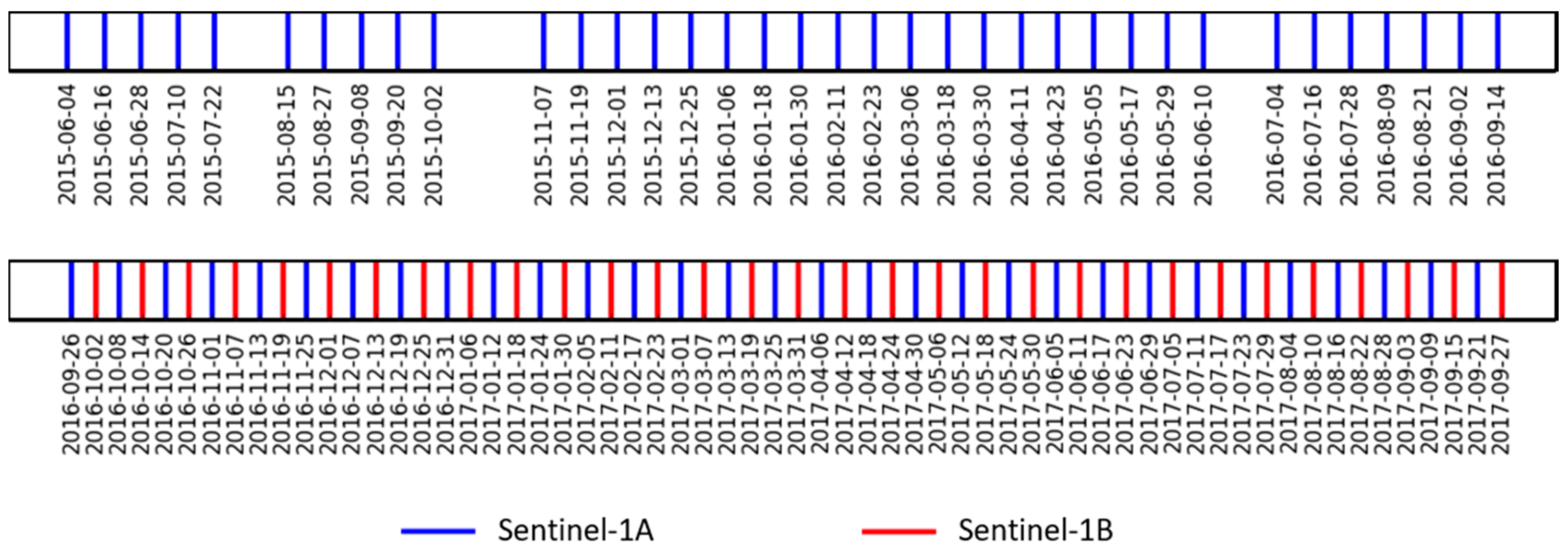
The Sentinel-1 mission provides data from a dual-polarization C-band Synthetic Aperture Radar (SAR) instrument. In this study, we use both Sentinel-1A and Sentinel-1B backscatter data, with a resolution of 10 m and a temporal resolution of 12 days, for each satellite. Previous studies have shown that VV (vertical–vertical) polarization data, in comparison to VH (vertical–horizontal) polarization, show high sensitivity to soil moisture [37,38,39,40,41,42]. VH data, in its turn, has a higher sensitivity to volume scattering, which depends strongly on the geometrical alignment and characteristics of the vegetation. Thus, VH data has a limited potential for the estimation of soil moisture compared to VV data, but higher sensitivity to vegetation [38,43,44]. Since irrigation makes a difference for vegetation density, and in order to make full use of the satellite data, we use both VV and VH polarizations for our analysis. The period of Sentinel-1A is from June 2015 until September 2017, while Sentinel-1B is available from September 2016 until September 2017. The database is shown in Figure 1. All of the Sentinel-1 data was pre-processed using the Sentinel-1 Toolbox, in three steps:
- -
- Thermal noise removal
- -
- Radiometric calibration
- -
- Terrain correction using SRTM (Shuttle Radar Topography Mission) DEM (Digital Elevation Model) at 30 m.
2.1.2. Ground Truth (SIGPAC)
The Geographic Information System for Agricultural Parcels (hereinafter SIGPAC) is a public registry of an administrative nature that contains information on the parcels [45]. The supplied SIGPAC plotter contains both graphical and alphanumeric information. The graphic information includes the referenced geographic boundary of each plot of land. Alphanumeric information contains information about each one of the enclosures such as identification codes, surface area, land usage (updated annually), irrigation coefficient, average slope, and others. Information can be found on the website: http://sig.gencat.cat/visors/Agricultura.html [46].
In this study, the SIGPAC data is used as ground truth to validate our classification results with information regarding the land usage and irrigation coefficient.
2.2. Study Area
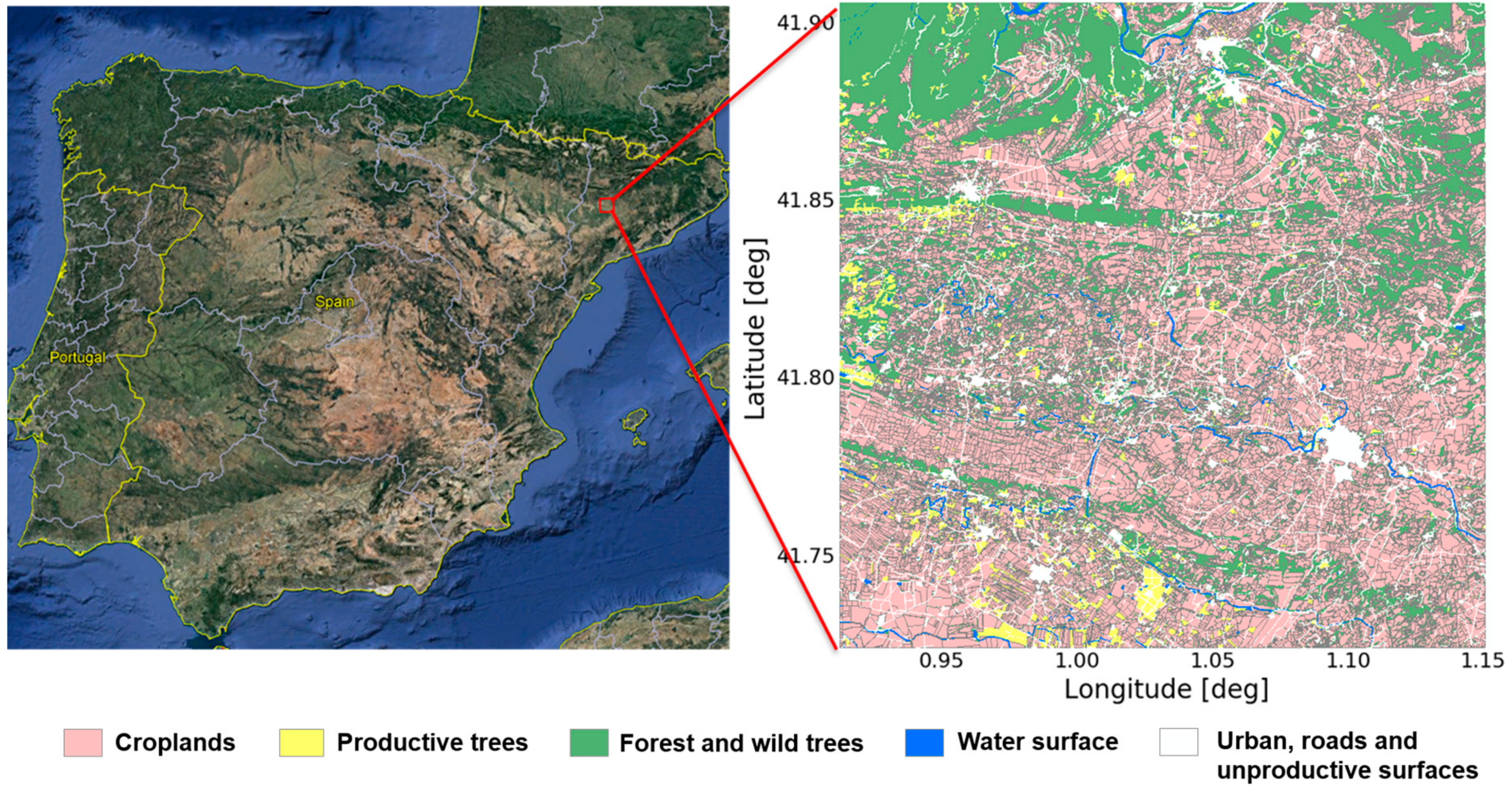
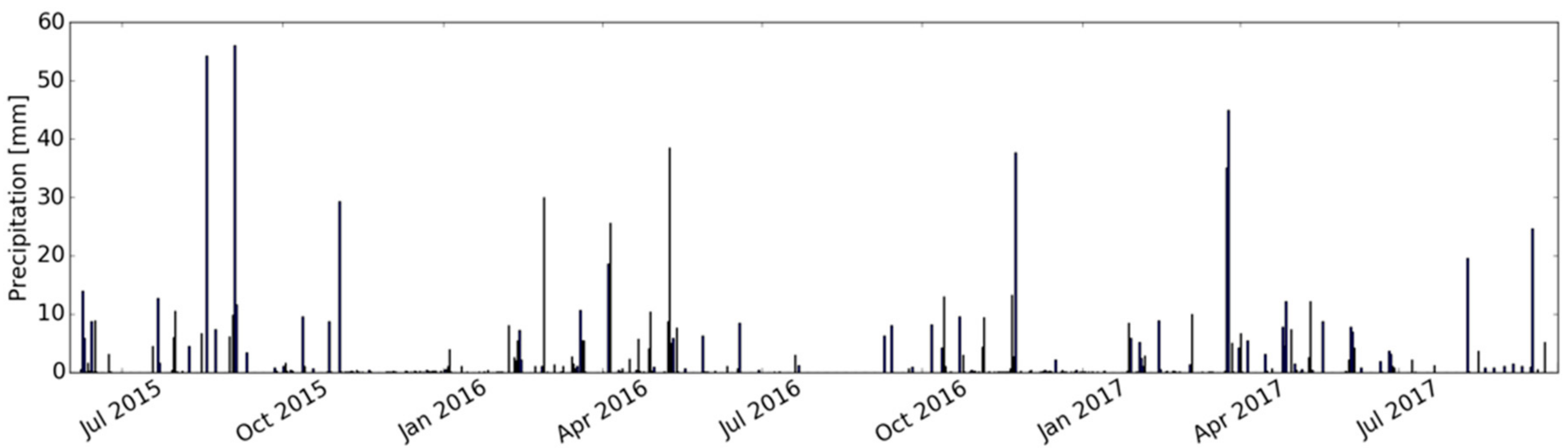
The study area covers a 20 km by 20 km area, located in Urgell, Catalonia, Spain (Figure 2). The Urgell climate is typically Mediterranean, with continental influence; it is mild in winter and warm in summer, with a very dry season in summer and two rainier seasons in autumn and spring [47]. The average annual precipitation is around 376 mm (347 mm in 2015, 385 mm in 2016, and 397 mm in 2017). Precipitation events at the Baldomar meteo station, which is the nearest one to our study area, are illustrated in Figure 3.
The study area is mainly irrigated using two irrigation methods: inundation, which is the old irrigation method, and sprinkler or drip, which are the new irrigation systems. The status of the irrigation is mostly static from year to year. Fields that have access to water are always irrigated, and fields that do not have access to water are not. In the old irrigated district, the open channel leads water into the agricultural fields, which causes vegetation flourishing in this area (lower left of the study area). Surrounding the irrigated area, the land is much drier without irrigation. Currently, a new irrigated system is being developed, surrounding the old irrigated system, using sprinkler or dripping irrigation; scatter irrigation fields are located in the middle and north of the study area. The irrigation period mainly occurs in summer, from May to September, and the frequency depends on the irrigation district. In the old district, the irrigation frequency is mainly every two weeks, and in the new area it may be daily, but it depends on the farmers.
In the fields with the new irrigation method, the drippers are always used to irrigate fruit trees, and the sprinkler is always used to irrigate crops. In our study, the fields are separated into irrigated trees, irrigated crops, and non-irrigated fields in the end.
Figure 2 shows the land-use map from SIGPAC in our study area. The croplands dominate most parts of the area, including wheat, corn, and alfalfa. The croplands include fields irrigated using inundation, sprinkler, or subsurface drippers, and rainfed fields. The productive trees are mainly fruit trees, olive trees, or vineyards. Forest and wild trees are spreading throughout the whole area, mostly in the mountainous places in the northwest part. In total, there are 22,775 fields of croplands and 3659 fields of productive trees that are used for the mapping and validation.
3. Methodology
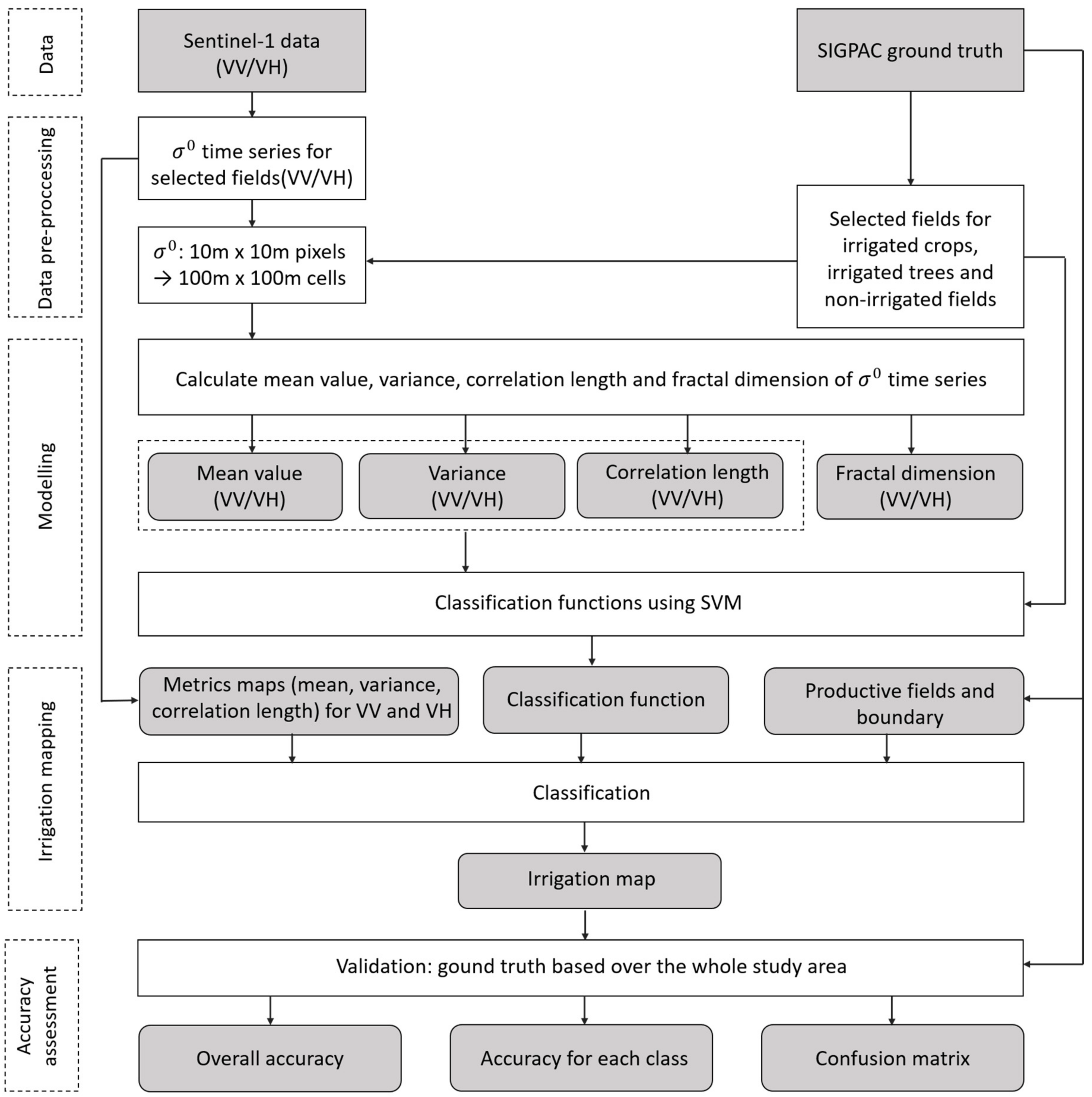
The first step is the data pre-processing. Second, we use metrics of a backscatter signal time series over the selected fields to perform modeling to build the classification function. Third, irrigation mapping is performed using the metrics maps, the classification function, and the fields boundary information. The accuracy assessment will be explained in the next section. The overall workflow using the Support Vector Machine (SVM) is shown in Figure 4.
3.1. Data Pre-Processing
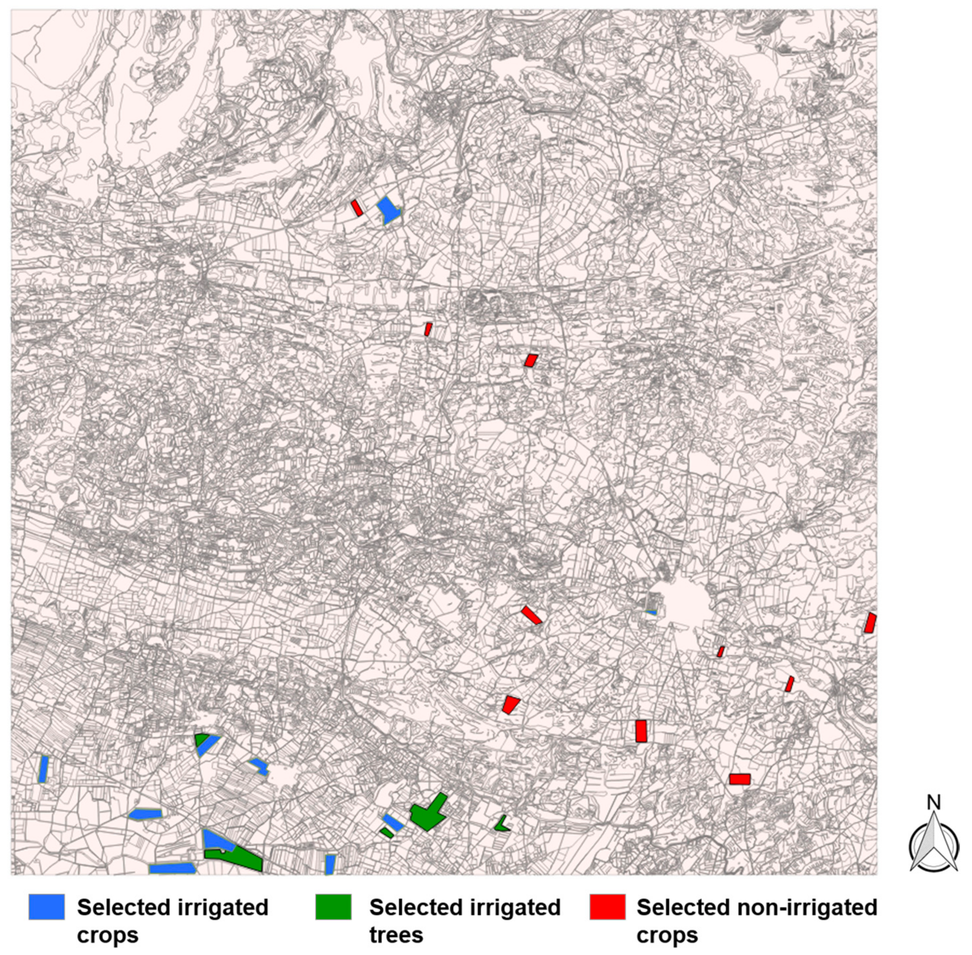
To build the classification method, we first selected 10 areas for irrigated crops, five areas for irrigated trees, and 10 areas for non-irrigated crop lands, as shown in Figure 5, to perform learning and modeling. The surface size of the selected areas varies from 3 ha to 25 ha. All of the pixels within the selected reference areas are pre-processed by averaging every 10 by 10 pixels, starting from the left-top corner into 100 m by 100 m cells in order to reduce the speckle effect.
3.2. Analyzed Metrics
The mathematical statistics of the backscatter time series for the selected areas, including irrigated trees, irrigated croplands, and non-irrigated crops, will be analyzed. In principle, the backscatter values are different for irrigated and non-irrigated areas and for different irrigation methods, since different water content in the soil creates differences in soil dielectric constant, which relates to the backscatter characters. Furthermore, the irrigation makes a difference for vegetation density, which affects the backscatter coefficient, especially for VH polarization. Additionally, the changing pattern and other mathematical statistics will be analyzed for irrigated trees, irrigated crops, and non-irrigated crops.
Analysis of the temporal-related metrics is the first step in the analysis of the possibility that the three types of classes will be separated. The analyzed metrics include the mean value of the backscatter time series, the temporal variance of the signal, the signal correlation length, and the fractal dimension. First, we analyze these metrics solely within the selected areas over irrigated croplands, irrigated trees, and non-irrigated crops. Cells with hundred-meter resolution fell into the selected fields are considered for the analysis.
3.2.1. Mean Value of σ°
The mean value, which is the basic statistical parameter of a time series, shows the average scale of the data. In the first analysis, the mean value of the backscatter time series is taken for each 100-m cell within the selected irrigated and non-irrigated areas. Analysis is based on the whole period of our data acquisition, as shown in Figure 1. The mean value reflects the general level of signal intensity for different land use.
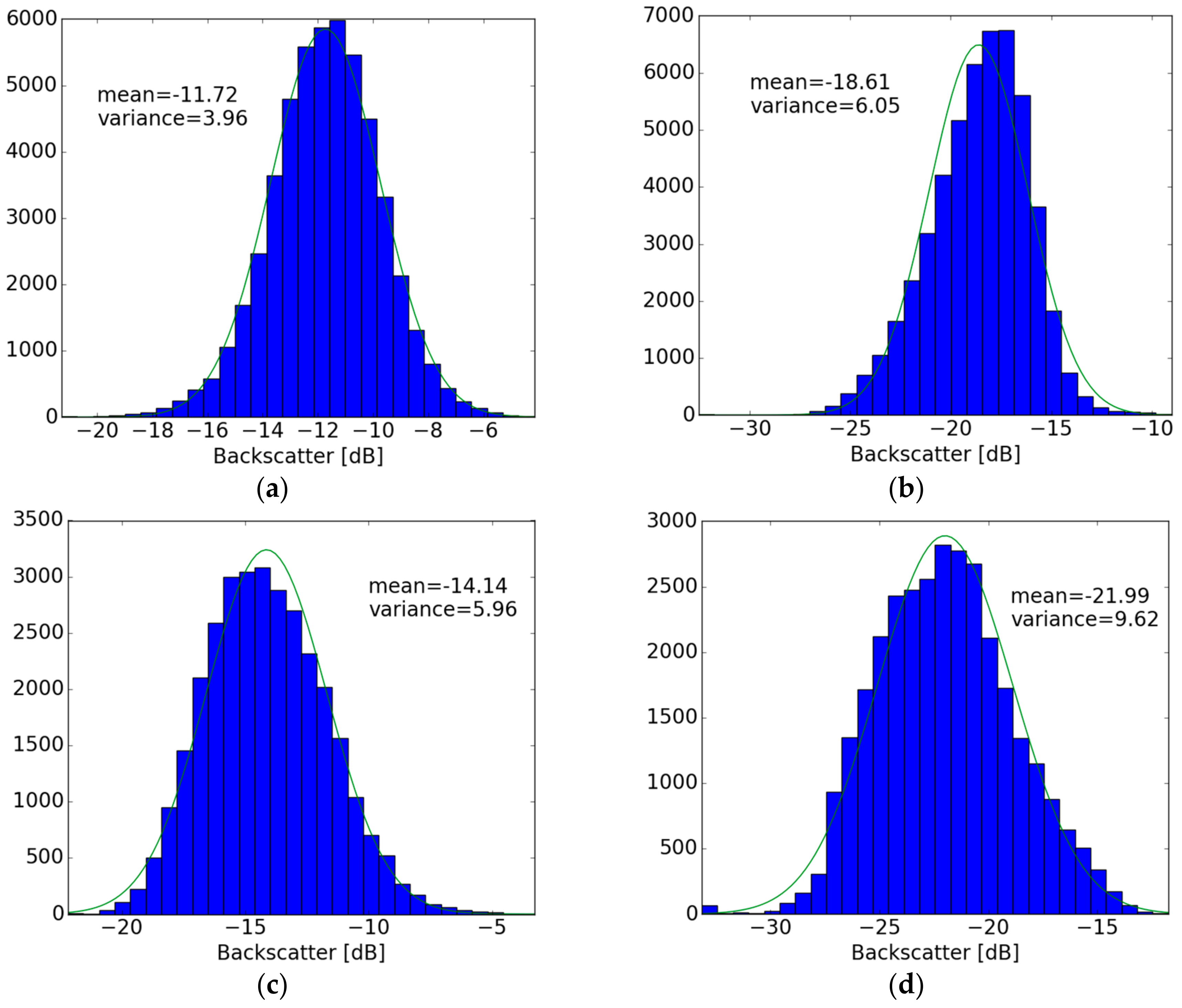
For VV polarization, the backscatter intensity should be higher for irrigated than non-irrigated fields, with more water content in the fields because the increase of water increases reflectivity and thus, the backscatter value. For VH polarization, the sensitivity to water content in the soil is less pronounced, while the impact of vegetation increases. Figure 6 illustrates the case of VV and VH polarization signal dynamics through radar signal histograms; the approximate mean value of the selected irrigated cells for VV polarization is −11.724 dB, as shown in Figure 6a, and −14.137 dB for non-irrigated cells, as shown in Figure 6b. The mean values are smaller for VH polarization than VV polarization, and smaller for non-irrigated fields than irrigated fields.
3.2.2. Signal Variance
Variance is the expectation of the squared deviation of a random variable from its mean. Informally, it measures how far a set of numbers is spread out from its average value. The variance value over the forest and urban areas are expected to be lower over the agricultural areas, with limited temporal variations. Figure 6 shows that the variance values are smaller for irrigated areas compared with non-irrigated areas, while VH polarization shows in average higher values than VV polarization, but similarly to VV, it is also smaller for the irrigated area.
3.2.3. Signal Correlation Length
Autocorrelation is a measure of the internal correlation within a time series. Autocorrelation is the correlation of a signal (μ) with a delayed copy of itself as a function of delay (τ). It is a way of measuring and explaining the internal association between observations in a time series.
ρ(τ) = E [ƒ(μ) ƒ (μ − τ)],
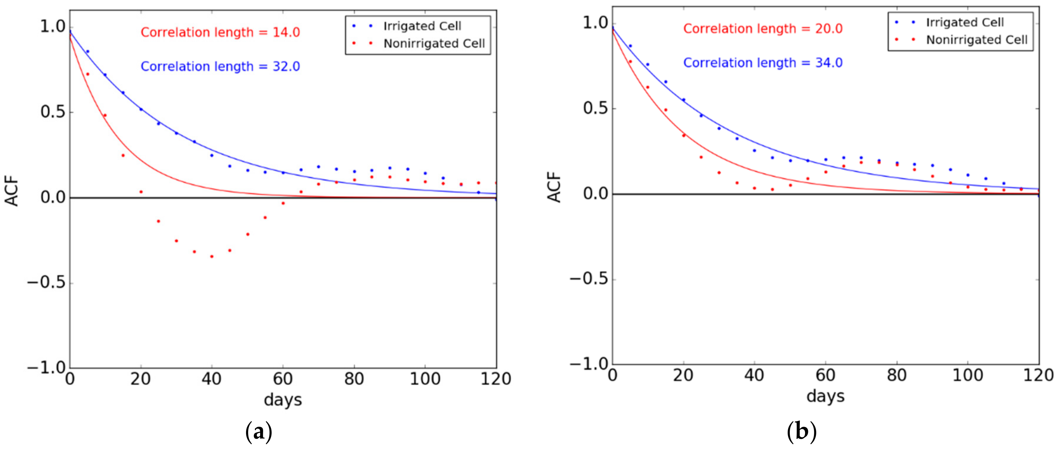
Autocorrelation length represents the temporal interval in which the autocorrelation function decays to half of the power the fastest. It provides the information regarding the temporal variance of the backscatter signal, with limited values for fast-changing fields (e.g., irrigated fields) in principle. In our analysis, Edelson and Krolik’s Discrete Correlation Function (DCF) is used [48]. Figure 7 gives two examples for irrigated cells and non-irrigated cells for VV and VH polarization; an exponential function [y = A exp(x/B)] is used to fit the temporal discrete correlation function. The correlation length is larger for irrigated cells in this case, since the existence of temporal variations is linked principally to soil moisture dynamic, and for non-irrigated areas, local temporal variations due to roughness and vegetation could generate reduction on correlation length; however, the overall results show that a large range of autocorrelation length varies from less than 10 days to more than 60 days for both irrigated and non-irrigated cells.
3.2.4. Fractal Dimension
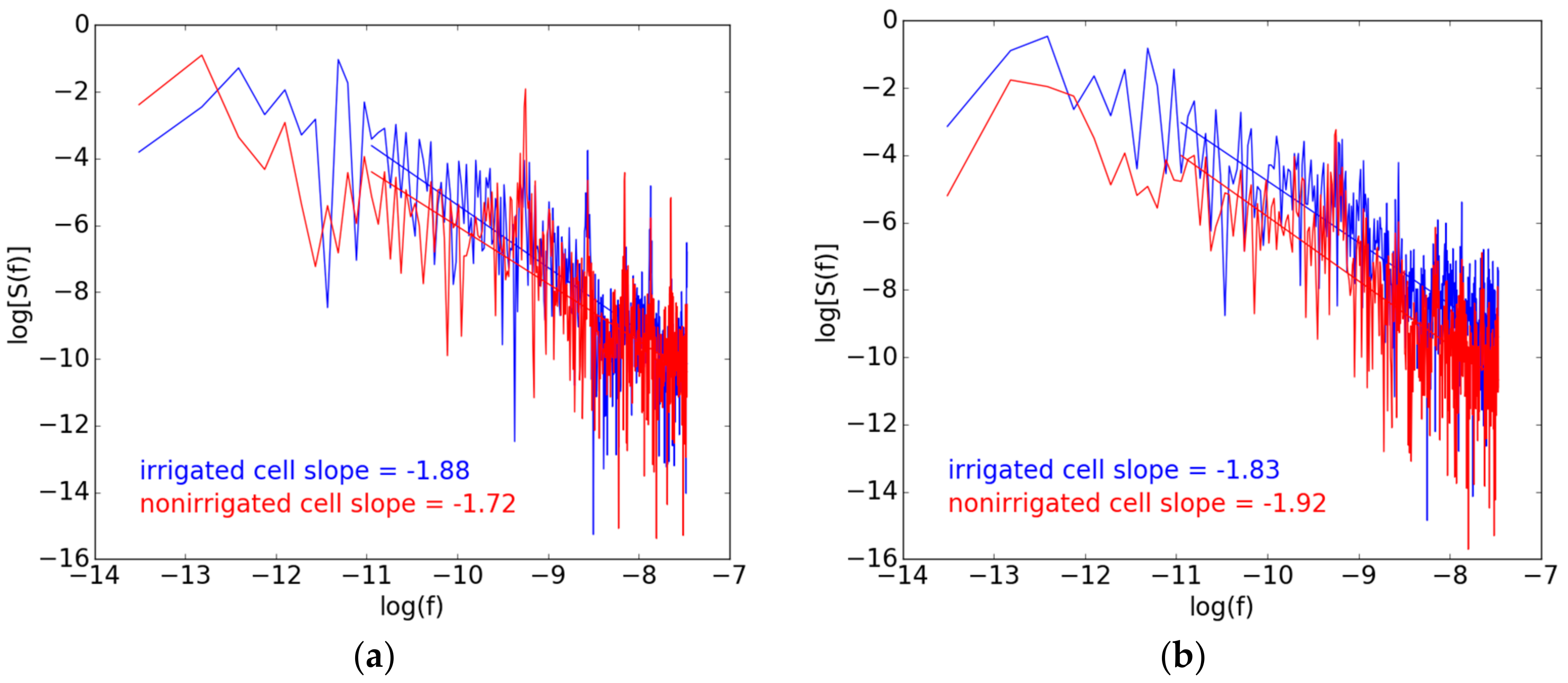
To quantitatively characterize backscatter dynamics, fractal geometry can be used to extract robust features hidden in the fluctuations. Fractals have the property of self-similarity [49,50,51]. Our fractal characterization is based on the power spectrum dependence of a fractional Brownian motion. We determine the power spectrum of the backscatter time series by computing its Fourier transform. The scaling behavior of the data is revealed by a power-law dependence of the spectrum as a function of frequency [52,53]:
S(f) ≈ 1/f β
The fractal dimension is derived from the slope β of a least-squares regression linear fit to the data points in the log–log plot of the power spectrum, leading to the dimension [50]: D = 7/2 − β/2.
Over irrigated fields, the fractal dimensions are expected to be higher in principle, since irrigation should bring faster change in the irrigation period to SAR signals. However, the results show that the values are almost the same for irrigated and non-irrigated fields, since the backscatter is influenced by many factors, including soil roughness and precipitation. Figure 8 provides two examples of power spectral density plots of irrigated cells and non-irrigated cells for VV and VH polarization. The difference of slopes is not evident for the separation of irrigated and non-irrigated fields. In the implementation of our method, we discard fractal dimensions, which are not robust enough for classification.
3.3. Modeling
3.3.1. Support Vector Machine
A Support Vector Machine (SVM) is a typical learning machine for two-group classification problems [54]. SVM is a discriminative classifier that is formally defined by a separating hyperplane. In other words, given labeled training data (supervised learning), the algorithm builds an optimal hyperplane, which can be used to categorize a new dataset. In a two-dimensional space, the hyperplane becomes a line dividing a plane into two classes, which lay in each part of the plane. Our method of separating non-irrigated fields, irrigated crops, and irrigated trees is based on the linear Support Vector Machine.
In our process, first, we separate irrigated and non-irrigated fields using mean value and variance, then, the irrigated fields are further separated into irrigated trees and irrigated crops using variance and correlation length. The reason to separate two classes each time instead of three is that the mean values of irrigated trees and irrigated crops are a bit mixed, since the backscatter difference between the flouring crops and trees are not evident, and the correlation length for non-irrigated crops varies a lot depending on the soil roughness and vegetation status, which makes it difficult to be separated from irrigated fields.
3.3.2. Classification Function
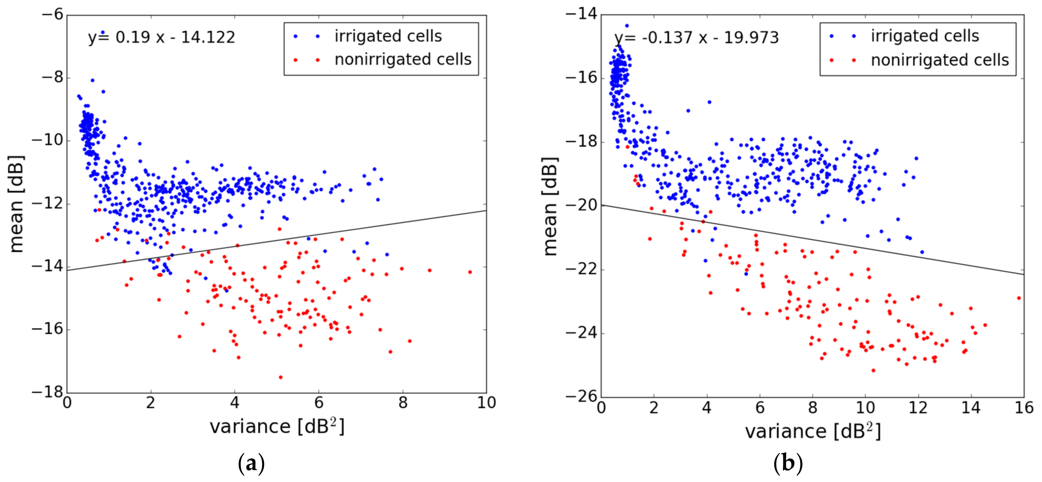
The classification functions are derived using SVM as shown in Figure 9 and Figure 10. First, a function for the irrigated fields and non-irrigated fields classification is built by the mean value and variance. Second, a function for irrigated crops and irrigated trees classification is built by the variance and correlation length.
Considering the selected irrigation and non-irrigated masks, we analyzed the mean value and the variance of the backscatter time series for each 100 m by 100 m cell. The results are shown in Figure 9. The mean values can be easily distinguished for irrigated and non-irrigated cells, with large values for irrigated cells. Over the selected fields, the mean variance for VV polarization is 3.96 dB for irrigated areas and 5.96 dB for non-irrigated areas. The function of the VV polarization increases, while for the VH polarization, it decreases, because VV is more sensitive to soil moisture and VH is more sensitive to vegetation.
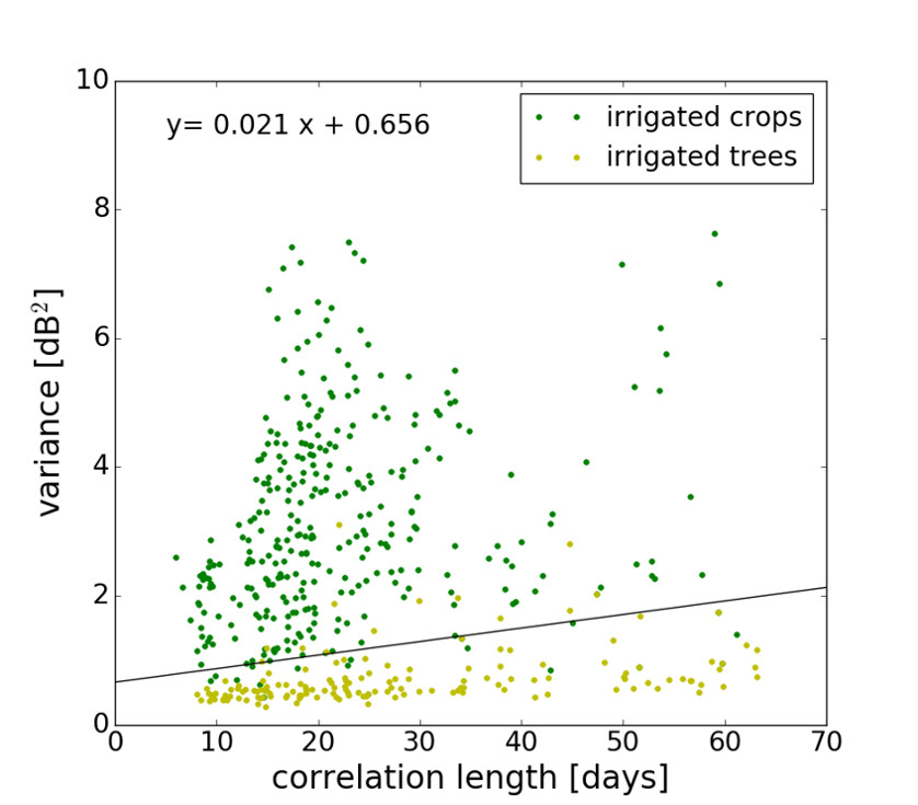
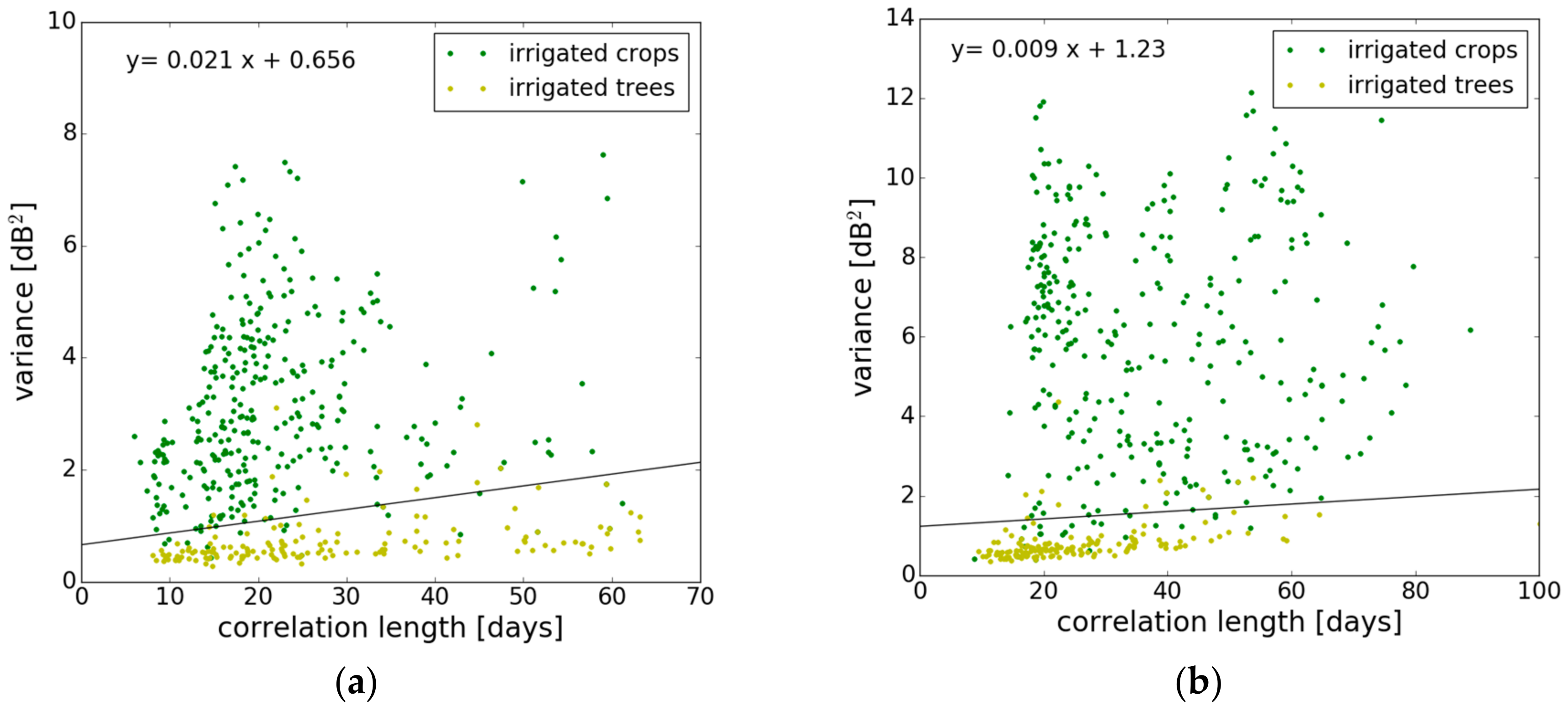
Based on the two metrics, the irrigated and non-irrigated fields can be separated by the function of the mean value and the variance, using both VV and VH polarization. Then, for irrigated areas, the SVM derived linear function of correlation length and variance is used for the separation of the irrigated trees and irrigated crops (as shown in Figure 10). The characteristics of its self-correlation vary substantially, as shown in Figure 10. The effect of vegetation coverage limits the variance for the case of trees. Apart from this, we see a limited increase of variance with correlation length.
By using the function of the correlation length and variance, we can separate irrigated crops and irrigated trees.
3.4. Tree Classification
Our study uses a tree classification, considering metrics from both VV and VH polarization, including mean value, variance, and autocorrelation length. Over the whole study area, the two linear SVM functions in Figure 9 are first used to separate irrigated fields and non-irrigated fields. Second, the two linear SVM functions in Figure 10 are used to separate irrigated crops and irrigated trees.
3.5. Random Forest (RF) Classification
Random Forest (RF) is an ensemble learning method for classification, regression, and other tasks, that operates by constructing a multitude of decision trees at training time and outputting the class that is the type of the classes (classification) or mean prediction (regression) of the individual trees [55,56].
Our study targets the classification process using half of the fields for learning, and the other half for validating, with the mean value, the variance, and autocorrelation length of both VV and VH polarization as input.
4. Results and Validation
With the geoinformation from SIGPAC, we know the boundary of all of the fields in our study area, which changed very slightly over the study period. The latest version of the fields’ boundary is used. The surface area of the fields varies from less than 0.5 ha to more than 50 ha.
To apply our method over the whole study area, we average the backscatter into each field, so the speckle effect can be reduced. Instead of validating a 100-m resolution map, we validated the backscatter at each field scale to be consistent with the ground truth. Some of our fields are smaller than the 100 m by 100 m size, so it makes more sense to consider a field scale for which we have ground information.
4.1. Metrics Mapping
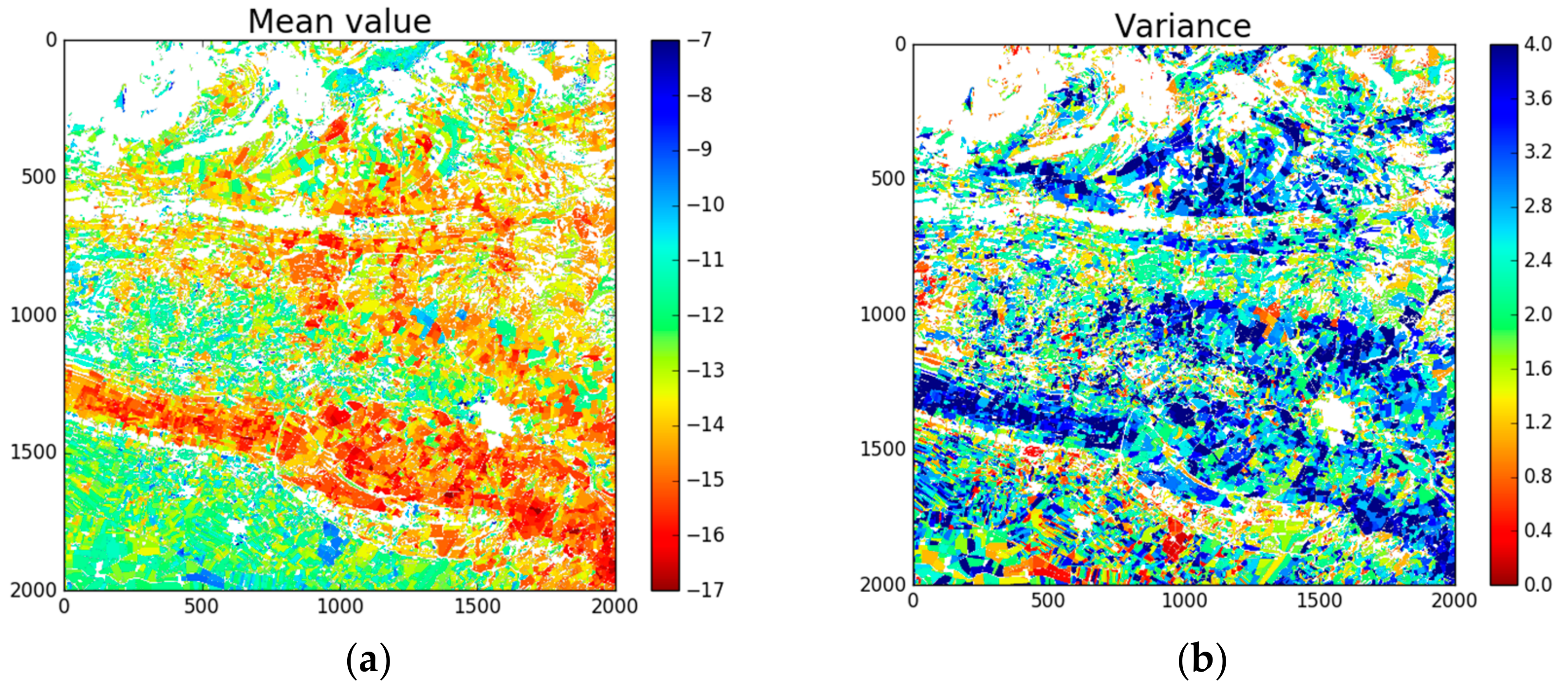
For each segmented field, we calculate these four metrics using the averaged backscatter signals for both VV and VH polarization. The maps of mean value, variance, correlation length, and fractal dimension for VV polarization over the study area are shown in Figure 11. Areas including forests, urban areas, and water bodies are masked out, so all of the productive fields are left to be illustrated. In the mean value map, areas with low values relate to non-irrigated fields, which can be easily distinguished from the irrigated fields. The same case exists in the variance map, where areas with high values relate to non-irrigated fields. In the correlation length map, the non-irrigated fields have relatively lower values, but it is becoming more difficult to separate them from the irrigated fields. Finally, the fractal dimension map shows a mixed situation for these two classes, which we therefore decided not to use.
4.2. Classification Map
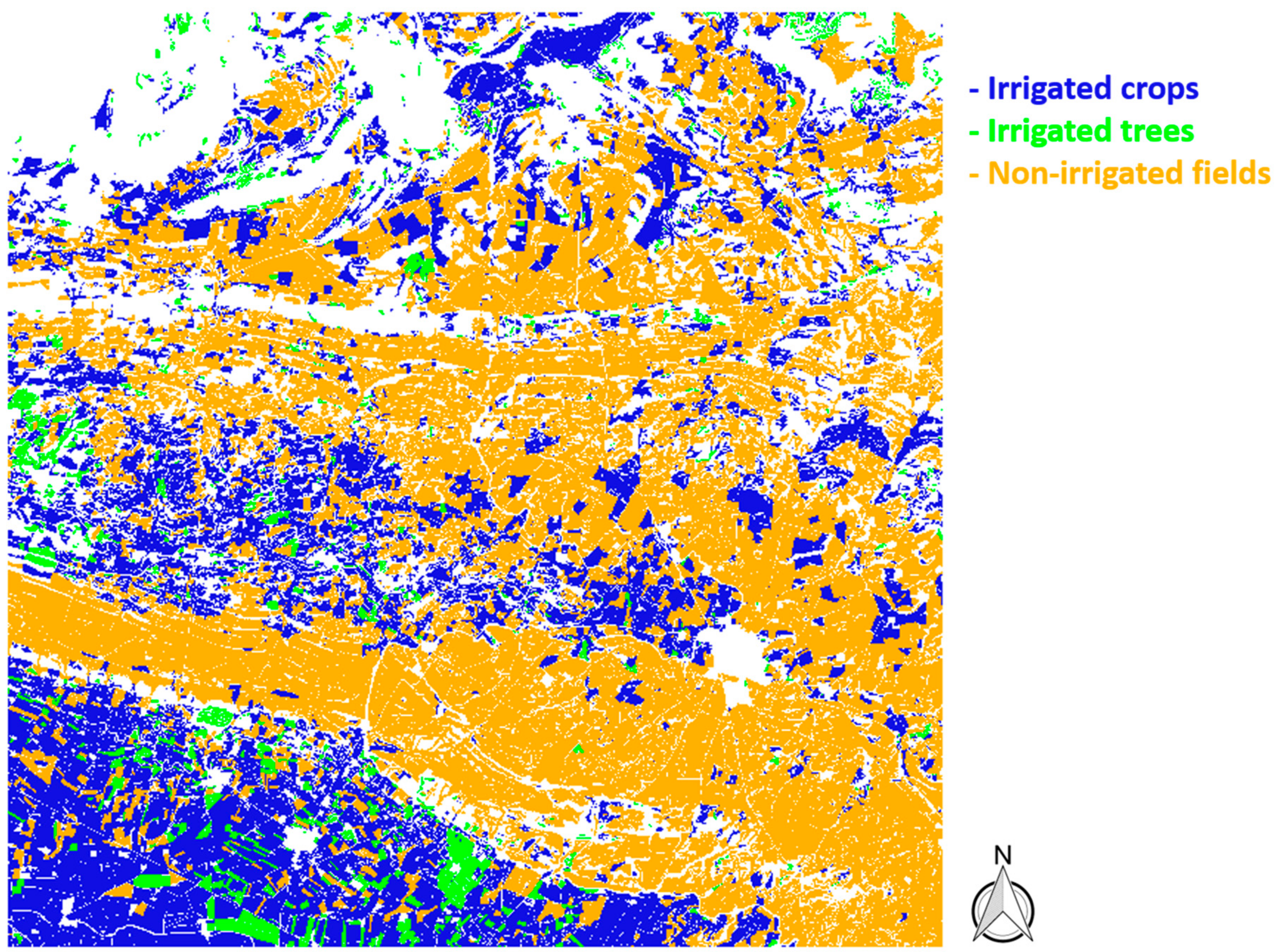
Using the tree classification method based on the SVM with the mean value, variance, and correlation length for both VV and VH polarization as input, three classes, including non-irrigated fields, irrigated crops, and irrigated trees are classified after masking out forest, urban areas, and water bodies, as shown in Figure 12. The blue color represents the irrigated croplands, while the green color represents the irrigated trees. Yellow-colored areas are classified as non-irrigated fields.
4.3. Validation
Validation is done using SIGPAC information over all of the productive fields in our study area (26,434 fields in total). Each field is checked if it is correctly classified through being compared with the ground truth. The confusion matrix is listed in Table 1.
The overall accuracy, which is the ratio of correctly classified fields and the total number of fields, is 81.08%, with the accuracy for non-irrigated crops slightly higher, with a value of 83.27%. The accuracy for irrigated crops is 77.53%, while for irrigated trees, it is 73.49%.
The most wrongly classified fields are irrigated crops into non-irrigated fields, with a percentage of 20.6%. The crops are mainly wheat. The different types of irrigation techniques may be a reason for the error, since fields using a new irrigated system are irrigated daily, while fields in the old irrigation area are irrigated about every two weeks, which makes the contribution of the irrigation events to the signal less important. The non-irrigated fields that were wrongly classified into irrigated crops were also high, with a percentage of 14.5%; most of them are located in the mountainous areas, where they may be influenced by topography. For irrigated trees, the most wrongly classified was into irrigated crops, which are the green-colored fields, with a percentage of 22.3%. The difference in the behaviors of backscatter signals for irrigated trees and very flouring crops may not be very evident.
The RF classification is also tested using half of the fields for learning and the other half for validating. The overall accuracy is around 82.2%, with the tree depth at three. The result shows the best accuracy for the irrigated crop, followed by irrigated trees and non-irrigated crops, which is the worst. The accuracy may vary from 80% to 83% when using different ground truth fields for learning, since RF is a very sensitive method. When using mean value alone as the input feature, the accuracy is about 80.9%, and using variance alone, the accuracy is about 66.4%, while when using correlation length alone, the accuracy is about 70.3%. Table 2 shows an example when using different combinations of metrics as input for RF classification. Combined the mean value with the variance, the accuracy increased by 1% above using the mean value only. After adding the correlation length, the accuracy increased by 0.3%.
5. Discussions
This study uses Sentinel-1 SAR multi-temporal data from June 2015 to September 2017 and focused on the statistics and metrics including the mean value, the variance, the correlation length, and the fractal dimension. In the classification, only the first three metrics are used as input. The SVM and RF are tested, and both methods showed a good accuracy.
The mean value shows a clear difference for irrigated and non-irrigated fields in VV polarization, as shown in Figure 11a. The non-irrigated fields have smaller mean values of the backscatter time series than irrigated fields, because of the backscatter signal intensity increasing with the soil dielectric constant, which is proportional to the water content in the soil until it is flooded.
The variance values of non-irrigated fields are relatively higher than those for irrigated fields, as shown in Figure 6, Figure 9 and Figure 11b. This behavior is because non-irrigated areas can generally reach extreme values, with high levels due to precipitation events, and extremely low values in the summer period due to a long absence of precipitation. This is not the case for irrigated fields that receive water frequently, and they rarely reach those extreme low moisture levels. The variance values are somehow mixed, but we can still find the pattern, as the signals of non-irrigated areas tend to be more spread out. There is a class with dense blue points for irrigated fields with low variance values (less than 1 for both VV and VH) and high mean values (greater than −11 dB for VV and −18 dB for VH) in Figure 9, which consists of the irrigated trees, whose relatively high volumes yield higher reflectivity with small changes.
The function of the VV polarization increases, while for the VH polarization, it decreases as shown in Figure 9, because VV is more sensitive to soil moisture, and VH is more sensitive to vegetation. For VV polarization in a relatively dry region such as in our study area, small changes in soil moisture with a low variance value will have a relatively low average backscatter mean value, while the increase of soil moisture on some days will lead to a high variance value and a relatively high average mean value. However, for the irrigated trees, the vegetation volumes contribute more to the backscatter signal, which leads to higher mean values with low variances. The case for VH polarization, which is more sensitive to vegetation, is more complex. For irrigated fields, the trees always have a high backscatter mean value with small changes, and for crops, the increase of variance may due to the flourishing of the vegetation as a consequence of irrigation. This could also be due to the decrease of canopy caused by harvest events, which in the end leads to relatively stable backscatter mean values. For non-irrigated fields, the vegetation volume will not be able to reach to a very dense situation because of water shortage, so the increase of variance can only be the consequence of harvest events, which of course will lead to a low backscatter mean value.
The correlation length shows a relatively higher value for irrigated fields than non-irrigated fields, as shown in Figure 7 and Figure 11c. As the irrigation event happens in the summertime, the backscatter time series show a more seasonal pattern, which brings a higher correlation length value. Since the irrigation status is quite different for different croplands (different irrigation method, different irrigation period, different amount of applied water, etc.), the characteristics of its self-correlation may vary substantially, as shown in the x-axis of Figure 10.
The fractal dimension didn’t show a clear difference between irrigated fields and non-irrigated fields (Figure 8 and Figure 11d). The temporal backscatter signal is influenced by many factors such as the irrigation frequency, precipitation, the vegetation type, etc.; the self-similarity of the time series is hardly observed. We discarded it as input in the end.
For the classification step, we tested both the SVM and RF method, and both show good accuracy. In SVM classification, we use the linear SVM functions to separate irrigated fields and non-irrigated fields. Then, the irrigated fields are further separated into irrigated crops and irrigated trees. RF classification used half of the fields for learning and the other half for testing; the fields are also separated into irrigated crops, irrigated trees, and non-irrigated fields. RF can give a better accuracy with a larger number of ground truth fields for learning and a bigger tree depth. However, the accuracy of RF classification with the tree depth at three can change from 80% to 83% when using different fields for learning. Through increasing the input metrics, the RF method shows an increase of accuracy. The SVM method also gives a good accuracy, and is more robust. Besides, SVM does not need as many ground truth fields as RF, but of course, more ground truth fields may bring a better accuracy.
6. Conclusions
In this paper, a methodology for irrigation mapping using the Sentinel-1 SAR data time series is introduced. The backscatter mean value, the signal variance, and the correlation length are derived from the backscatter signal time series and are used for classification. The classification result of irrigated and non-irrigated fields is compared with the ground truth from SIGPAC database over 26,434 fields in the whole study area. The result shows a good overall accuracy, which is 81.08% using the SVM. The mean value of the backscatter time series is the key to separating irrigated and non-irrigated fields, while the correlation length and variance are used for the separation of irrigated trees and irrigated crops.
The results of the SVM show good accuracy for irrigated croplands and non-irrigated fields, with soil moisture change more dominant to multi-temporal radar signals. Classification results for irrigated trees are slightly poor, and the effect of vegetation cover over backscatter in the case of trees is more obvious than the effect of soil moisture change.
The RF classification gives a similar accuracy as SVM, but it depends a lot on the number and location of the ground truth fields for machine learning, and is less robust compared with SVM.
In areas where there is no ground field information available, instead of using field boundary information, field segmentation was performed using Sentinel-2 NDVI data [57,58,59], but only for areas without frequent cloud cover. Another alternative method is using 100-m resolution cells directly to calculate the metrics only from Sentinel-1 SAR data, which is more consistent with our original intention to use the methodology under any weather conditions.
This approach can be used in any agricultural areas when SAR data is available, and is adapted to regions with a limited use of S2 because of climate conditions. For areas that are more humid than the Catalunya study area during irrigation season, soil moisture contribution will be more limited, which may make the method less robust. Additionally, this method does not need to develop operational algorithms to estimate soil moisture before application; it is based directly on radar signal analysis. It is unrestricted by weather conditions and the location of the fields. The results demonstrated the potential of using Sentinel-1 data for irrigation mapping at the field scale.
Author Contributions
Q.G. and M.Z. conceived, designed and implemented the research. Q.G. coded and performed the analysis of the data and drafted the manuscript. M.J.E. assisted in the data analysis and interpretation. All authors reviewed and improved the manuscript. The study was supervised by M.Z.
Funding
Qi Gao received grant DI-15-08105 from the Spanish Education Ministry (MICINN) and DI-2016-078 from the Catalan Agency of Research (AGAUR). The study was partially funded by the REC project funded by the European Commission Horizon 2020 Programme for Research and Innovation (H2020) in the context of the Marie Skłodowska-Curie Research and Innovation Staff Exchange (RISE) action under grant agreement No. 645642.
Acknowledgments
The authors wish to thank the technical teams for their support and the SIGPAC team, which provides plenty of ground information.
Conflicts of Interest
The authors declare no conflict of interest.
References
- Gleick, P.H. Global freshwater resources: Soft-path solutions for the 21st century. Science 2003, 302, 1524–1528. [Google Scholar] [CrossRef] [PubMed]
- Rosegrant, M.W.; Meijer, S.; Cline, S.A. International Model for Policy Analysis of Agricultural Commodities and Trade (IMPACT): Model Description; IFPRI: Washington, DC, USA, 2002. [Google Scholar]
- Ozdogan, M.; Yang, Y.; Allez, G.; Cervantes, C. Remote Sensing of Irrigated Agriculture: Opportunities and Challenges. Remote Sens. 2010, 2, 2274–2304. [Google Scholar] [CrossRef] [Green Version]
- Kharrou, M.; Page, M.L.; Chehbouni, A.; Simonneaux, V.; Er-Raki, S.; Jarlan, L.; Ouzine, L.; Khabba, S.; Chehbouni, G. Assessment of Equity and Adequacy of Water Delivery in Irrigation Systems Using Remote Sensing-Based Indicators in Semi-Arid Region, Morocco. Water Resour. Manag. 2013, 27, 4697–4714. [Google Scholar] [CrossRef]
- Stefan, V. Mixed Modeling and Multi-Resolution Remote Sensing of Soil Evaporation. Ph.D. Thesis, Université Toulouse 3 Paul Sabatier (UT3 Paul Sabatier), Toulouse, France, 2016. [Google Scholar]
- Ambika, A.K.; Wardlow, B.; Mishra, V. Data descriptor: Remotely sensed high resolution irrigated area mapping in India for 2000 to 2015. Sci. Data 2016, 3, 160118. [Google Scholar] [CrossRef] [PubMed]
- Cai, X.; Magidi, J.; Nhamo, L.; Koppen, B. Mapping Irrigated Areas in the Limpopo Province, South Africa; IWMI Working Paper 172; IWMI: Colombo, Sri Lanka, 2017. [Google Scholar]
- Thenkabail, P.S.; Schull, M.; Turral, H. Ganges and Indus river basin land use/land cover (LULC) and irrigated area mapping using continuous streams of MODIS data. Remote Sens. Environ. 2004, 95, 317–341. [Google Scholar] [CrossRef]
- Beltran, C.M.; Belmonte, A.C. Irrigated crop area estimation using Landsat TM imagery in La Mancha, Spain. Photogramm. Eng. Remote Sens. 2001, 67, 1177–1184. [Google Scholar]
- Biggs, T.W.; Thenkabail, P.S.; Gumma, M.K.; Scott, C.A.; Parthasaradhi, G.R.; Turral, H.N. Irrigated area mapping in heterogeneous landscapes with MODIS time series, ground truth and census data, Krishna Basin, India. Int. J. Remote Sens. 2006, 27, 4245–4266. [Google Scholar] [CrossRef]
- Dheeravath, V.; Thenkabail, P.S.; Chandrakantha, G.; Noojipady, P.; Reddy, G.P.O.; Biradar, C.M.; Gumma, M.K.; Velpuri, M. Irrigated areas of India derived using MODIS 500 m time series for the years 2001–2003. ISPRS J. Photogramm. Remote Sens. 2009, 65, 42–59. [Google Scholar] [CrossRef]
- Kamthonkiat, D.; Honda, K.; Turral, H.; Tripathi, N.K.; Wuwongse, V. Discrimination of irrigated and rainfed rice in a tropical agricultural system using SPOT VEGETATION NDVI and rainfall data. Int. J. Remote Sens. 2005, 26, 2527–2547. [Google Scholar] [CrossRef]
- Draeger, W.C. Monitoring Irrigated Land Acreage Using LANDSAT Imagery: An Application Example. In Proceedings of the 11th International Symposium on Remote Sensing of Environment, Ann Arbor, MI, USA, 25–29 April 1977; pp. 515–524. [Google Scholar]
- Thiruvengadachari, S. Satellite sensing of irrigation pattern in semiarid areas: An Indian study. Photogramm. Eng. Remote Sens. 1981, 47, 1493–1499. [Google Scholar]
- Rundquist, D.C.; Richardo, H.; Carlson, M.P.; Cook, A. The Nebraska center-pivot inventory—An example of operational satellite remote sensing on a long term basis. Photogramm. Eng. Remote Sens. 1989, 55, 587–590. [Google Scholar]
- Akbari, M.; Mamanpoush, A.; Gieske, A.; Miranzadeh, M.; Torabi, M.; Salemi, H.R. Crop and land cover classification in Iran using Landsat 7 imagery. Int. J. Remote Sens. 2006, 27, 4117–4135. [Google Scholar] [CrossRef]
- Ozdogan, M.; Gutman, G. A New Methodology to Map Irrigated Areas Using Multi-Temporal MODIS and Ancillary Data: An Application Example in the Continental US. Remote Sens. Environ. 2008, 112, 3520–3537. [Google Scholar] [CrossRef]
- Boken, V.K.; Hoogenboom, G.; Kogan, F.N.; Hook, J.E.; Thomas, D.L.; Harrison, K.A. Potential of using NOAA-AVHRR data for estimating irrigated area to help solve an inter-state water dispute. Int. J. Remote Sens. 2004, 25, 2277–2286. [Google Scholar] [CrossRef] [Green Version]
- Xiao, X.; Boles, S.; Liu, J.; Zhuang, D.; Frolking, S.; Li, C.; Salas, W.; Moore, B., III. Mapping paddy rice agriculture in southern China using multi-temporal MODIS images. Remote Sens. Environ. 2005, 95, 480–492. [Google Scholar] [CrossRef]
- Xiao, X.; Boles, S.; Frolking, S.; Li, C.; Babu, J.Y.; Salas, W.; Moore, B. Mapping paddy rice agriculture in South and Southeast Asia using multi-temporal MODIS images. Remote Sens. Environ. 2005, 100, 95–113. [Google Scholar] [CrossRef]
- Gumma, M.K.; Thenkabail, P.S.; Hideto, F.; Nelson, A.; Dheeravath, V.; Busia, D.; Rala, A. Mapping Irrigated Areas of Ghana Using Fusion of 30 m and 250 m Resolution Remote-Sensing Data. Remote Sens. 2011, 3, 816–835. [Google Scholar] [CrossRef] [Green Version]
- Baghdadi, N.; Zribi, M. Land Surface Remote Sensing in Continental Hydrology; ISTE Press: London, UK; Elsevier: Oxford, UK, 2016. [Google Scholar]
- Morvan, A.L.; Zribi, M.; Baghdadi, N.; Chanzy, A. Soil moisture profile effect on radar signal measurement. Sensors 2008, 8, 256–270. [Google Scholar] [CrossRef] [PubMed]
- Anguela, T.P.; Zribi, M.; Hasenauer, S.; Habets, F.; Loumagne, C. Analysis of surface and root-zone soil moisture dynamics with ERS scatterometer and the hydrometeorological model SAFRAN-ISBA-MODCOU at Grand Morin watershed (France). Hydrol. Earth Syst. Sci. 2008, 12, 1415–1424. [Google Scholar] [CrossRef] [Green Version]
- Zribi, M.; Chahbi, A.; Shabou, M.; Lili-Chabaane, Z.; Duchemin, B.; Baghdadi, N.; Amri, R.; Chehbouni, A. Soil surface moisture estimation over a semi-arid region using ENVISAT ASAR radar data for soil evaporation evaluation. Hydrol. Earth Syst. Sci. 2011, 15, 345–358. [Google Scholar] [CrossRef] [Green Version]
- Zribi, M.; Gorrab, A.; Baghdadi, N. A new soil roughness parameter for the modelling of radar backscattering over bare soil. Remote Sens. Environ. 2014, 152, 62–73. [Google Scholar] [CrossRef] [Green Version]
- Fontanelli, G.; Paloscia, S.; Zribi, M.; Chahbi, A. Sensitivity analysis of X-band SAR to wheat and barley leaf area index in the Merguellil Basin. Remote Sens. Lett. 2013, 4, 1107–1116. [Google Scholar] [CrossRef] [Green Version]
- Zribi, M.; Dechambre, M. A new empirical model to retrieve soil moisture and roughness from C-band radar data. Remote Sens. Environ. 2003, 84, 42–52. [Google Scholar] [CrossRef]
- Baghdadi, N.; Cresson, R.; Pottier, E.; Aubert, M.; Zribi, M.; Jacome, A.; Benabdallah, S. A potential use for the C-band polarimetric SAR parameters to characterize the soil surface over bare agriculture fields. IEEE Trans. Geosci. Remote Sens. 2012, 50, 3844–3858. [Google Scholar] [CrossRef] [Green Version]
- Srivastava, H.S.; Patel, P.; Manchanda, M.L.; Adiga, S. Use of multiincidence angle RADARSAT-1 SAR data to incorporate the effect of surface roughness in soil moisture estimation. IEEE Trans. Geosci. Remote Sens. 2003, 41, 1638–1640. [Google Scholar] [CrossRef]
- Sikdar, M.; Cumming, I. A modified empirical model for soil moisture estimation in vegetated areas using SAR data. In Proceedings of the 2004 IEEE International Geoscience and Remote Sensing Symposium, Anchorage, AK, USA, 20–24 September 2004. [Google Scholar]
- Tomer, S.K.; Al Bitar, A.; Sekhar, M.; Zribi, M.; Bandyopadhyay, S.; Sreelash, K.; Sharma, A.K.; Corgne, S.; Kerr, Y. Retrieval and Multi-scale Validation of Soil Moisture from Multi-temporal SAR Data in a Tropical Region. Remote Sens. 2015, 7, 8128–8153. [Google Scholar] [CrossRef]
- Gao, Q.; Zribi, M.; Escorihuela, M.J.; Baghdadi, N. Synergetic use of Sentinel-1 and Sentinel-2 data for soil moisture mapping at 100 m resolution. Sensors 2017, 17, 1966. [Google Scholar] [CrossRef] [PubMed]
- El Hajj, M.; Baghdadi, N.; Zribi, M.; Bazzi, H. Synergic Use of Sentinel-1 and Sentinel-2 Images for Operational Soil Moisture Mapping at High Spatial Resolution over Agricultural Areas. Remote Sens. 2017, 9, 1292. [Google Scholar] [CrossRef]
- Ribbes, F.; Toan, T.L. Rice field mapping and monitoring with RADARSAT data. Int. J. Remote Sens. 1999, 20, 745–765. [Google Scholar] [CrossRef]
- Shao, Y.; Fan, X.; Liu, H.; Xiao, J.; Ross, S.; Brisco, B.; Brown, R.; Staples, G. Rice monitoring and production estimation using multitemporal RADARSAT. Remote Sens. Environ. 2001, 76, 310–325. [Google Scholar] [CrossRef]
- Zribi, M.; Andre, C.; Decharme, B. A Method for Soil Moisture Estimation in Western Africa Based on the ERS Scatterometer. IEEE Trans. Geosci. Remote Sens. 2008, 46, 438–448. [Google Scholar] [CrossRef]
- Patel, P.; Srivastava, H.S.; Panigrahy, S.; Parihar, J.S. Comparative evaluation of the sensitivity of multi-polarized multi-frequency SAR backscatter to plant density. Int. J. Remote Sens. 2006, 27, 293–305. [Google Scholar] [CrossRef]
- Jacome, A.; Bernier, M.; Chokmani, K.; Gauthier, Y.; Poulin, J.; De Sève, D. Monitoring Volumetric Surface Soil Moisture Content at the La Grande Basin Boreal Wetland by Radar Multi Polarization Data. Remote Sens. 2013, 5, 4919–4941. [Google Scholar] [CrossRef] [Green Version]
- Amazirh, A.; Merlin, O.; Er-Raki, S.; Gao, Q.; Rivalland, V.; Malbeteau, Y.; Khabba, S.; Escorihuela, M.J. Retrieving surface soil moisture at high spatio-temporal resolution from a synergy between Sentinel-1 radar and Landsat thermal data: A study case over bare soil. Remote Sens. Environ. 2018, 211, 321–337. [Google Scholar] [CrossRef]
- Eweys, O.A.; Elwan, A.; Borham, T. Retrieving topsoil moisture using RADARSAT-2 data, a novel approach applied at the east of The Netherlands. J. Hydrol. 2017, 555, 670–682. [Google Scholar] [CrossRef]
- Gherboudj, I.; Magagi, R.; Berg, A.A.; Toth, B. Soil moisture retrieval over agricultural fields from multi-polarized and multi-angular RADARSAT-2 SAR data. Remote Sens. Environ. 2011, 115, 33–43. [Google Scholar] [CrossRef]
- Karjalainen, M.; Kaartinen, H.; Hyyppä, J.; Laurila, H.; Kuittinen, R. The Use of ENVISAT Alternating Ploarization SAR Images in Agricultureal Monitoring in Compatison with RADARSAT-1 SAR Images. In Proceedings of the ISPRS Congress, Istanbul, Turkey, 12–23 July 2004. [Google Scholar]
- Chauhan, S.; Srivastava, H.S. Comparative evaluation of the sensitivity of multi-polarized SAR and optical data for various land cover classes. Int. J. Adv. Remote Sens. GIS Geogr. 2016, 4, 1–14. [Google Scholar]
- INFORMACIÓ DE LES DADES SIGPAC. Available online: https://analisi.transparenciacatalunya.cat/api/views/w9bf-jejh/files/36948005-55ef-4003-826b-d01c17968ddf?download=true&filename=Dades_SIGPAC_2017.pdf (accessed on 1 May 2018).
- El Departament d’Agricultura, Ramaderia, Pesca i Alimentació (DARP)—Mapa Agricultura. Available online: http://sig.gencat.cat/visors/Agricultura.html (accessed on 1 May 2018).
- Escorihuela, M.J.; Quintana-Segui, P. Comparison of remote sensing and simulated soil moisture datasets in mediterranean landscapes. Remote Sens. Environ. 2016, 180, 99–114. [Google Scholar] [CrossRef]
- Edelson, R.A.; Krolik, J.H. The discrete correlation function—A new method for analyzing unevenly sampled variability data. Astrophys. J. 1988, 333, 646–659. [Google Scholar] [CrossRef]
- Mandelbrot, B.B. Fractals, Form, Chance and Dimension; W. H. Freeman and Company: San Francisco, CA, USA, 1977; p. 365. [Google Scholar] [CrossRef]
- Amri, R.; Zribi, M.; Lili-Chabaane, Z.; Duchemin, B.; Gruhier, C.; Chehbouni, A. Analysis of vegetation behavior in a north African semi-arid region, using SPOT-Vegetation NDVI data. Remote Sens. 2011, 3, 2568–2590. [Google Scholar] [CrossRef] [Green Version]
- Sun, W.; Xu, G.; Gong, P.; Liang, S. Fractal analysis of remotely sensed images: A review of methods and applications. Int. J. Remote Sens. 2006, 27, 4963–4990. [Google Scholar] [CrossRef]
- Menenti, M.; Azzali, S.; Vries, A.; Fuller, D.; Prince, S. Vegetation monitoring in southern Africa using temporal fourrier analysis of AVHRR/NDVI observations. In Proceedings of the International Symposium on Remote Sensing in Arid and Semi-arid Regions, Lanzhou, China, 25–28 August 1993; Volume 3, pp. 287–294. [Google Scholar]
- Havlin, S.; Amaral, L.A.N.; Ashkenazy, Y.; Golberger, A.L.; Ivanov, P.C.; Peng, C.K.; Stanley, H.E. Application of statistical physics to heartbeat diagnosis. Physica A 1999, 274, 99–110. [Google Scholar] [CrossRef] [Green Version]
- Vapnik, V.; Lerner, A. Pattern recognition using generalized portrait method. Autom. Remote Control 1963, 24, 774–780. [Google Scholar]
- Ho, T.K. Random Decision Forests. In Proceedings of the 3rd International Conference on Document Analysis and Recognition, Montreal, QC, Canada, 14–16 August 1995; pp. 278–282. [Google Scholar]
- Ho, T.K. The Random Subspace Method for Constructing Decision Forests. IEEE Trans. Pattern Anal. Mach. Intell. 1998, 20, 832–844. [Google Scholar] [CrossRef]
- Fukunaga, K.; Hostetler, L. The estimation of the gradient of a density function, with applications in pattern recognition. IEEE Trans. Inf. Theory 1975, 21, 32–40. [Google Scholar] [CrossRef]
- Comaniciu, D.; Meer, P. Mean shift: A robust approach toward feature space analysis. IEEE Trans. Pattern Anal. Mach. Intell. 2002, 24, 603–619. [Google Scholar] [CrossRef]
- Comaniciu, D.; Meer, P. Mean shift analysis and applications. In Proceedings of the Seventh IEEE International Conference on Computer Vision, Kerkyra, Greece, 20–27 September 1999; Volume 2, pp. 1197–1203. [Google Scholar]
Figure 1.
Temporal availability of Sentinel-1 time series data used in this study. Blue color indicates Sentinel-1A data and red color indicates Sentinel-1B data.
Figure 1.
Temporal availability of Sentinel-1 time series data used in this study. Blue color indicates Sentinel-1A data and red color indicates Sentinel-1B data.

Figure 2.
Study area located in Urgell, Catalunya, Spain, and the land-use map.

Figure 3.
Precipitation event in Baldomar meteo station (1.5 km away from the study area).

Figure 4.
Workflow overview using a Support Vector Machine (SVM).

Figure 5.
Selected reference areas for irrigated crops, irrigated trees, and non-irrigated crops.

Figure 6.
Signal backscatter distribution over selected irrigated areas for vertical–vertical (VV) polarization (a) and vertical–horizontal (VH) polarization (b); signal backscatter distribution over selected non-irrigated areas for VV polarization (c) and VH polarization (d).
Figure 6.
Signal backscatter distribution over selected irrigated areas for vertical–vertical (VV) polarization (a) and vertical–horizontal (VH) polarization (b); signal backscatter distribution over selected non-irrigated areas for VV polarization (c) and VH polarization (d).

Figure 7.
Autocorrelation function of irrigated and non-irrigated cells (100 m × 100 m) for VV polarization (a) and VH polarization (b).
Figure 7.
Autocorrelation function of irrigated and non-irrigated cells (100 m × 100 m) for VV polarization (a) and VH polarization (b).

Figure 8.
Power spectral density plots of irrigated and non-irrigated cells (100 m × 100 m) for VV polarization (a) and VH polarization (b).
Figure 8.
Power spectral density plots of irrigated and non-irrigated cells (100 m × 100 m) for VV polarization (a) and VH polarization (b).

Figure 9.
The relation of the mean value and the variance for irrigated and non-irrigated areas for VV polarization (a) and VH polarization (b).
Figure 9.
The relation of the mean value and the variance for irrigated and non-irrigated areas for VV polarization (a) and VH polarization (b).

Figure 10.
The relation of the variance and the correlation length for VV polarization (a) and VH polarization (b).
Figure 10.
The relation of the variance and the correlation length for VV polarization (a) and VH polarization (b).

Figure 11.
Examples of metrics maps for each field in VV polarization: mean value (a), variance value (b), correlation length (c), and fractal dimension (d).
Figure 11.
Examples of metrics maps for each field in VV polarization: mean value (a), variance value (b), correlation length (c), and fractal dimension (d).


Figure 12.
Irrigation mapping after masking out forest, urban areas, and water bodies.


Table 1.
Confusion matrix.
| Classes | Irrigated Crops | Irrigated Trees | Non-Irrigated Fields |
|---|---|---|---|
| Irrigated crops | 77.5% | 1.9% | 20.6% |
| Irrigated trees | 22.3% | 73.5% | 4.2% |
| Non-irrigated fields | 14.8% | 1.9% | 83.3% |
Table 2.
The accuracy with different input metrics.
| Input Metrics | Mean (VV/VH) | Mean (VV/VH) + Variance (VV/VH) | Mean (VV/VH) + Variance (VV/VH) + Correlation Length (VV/VH) |
|---|---|---|---|
| Accuracy | 80.9% | 81.9% | 82.2% |
© 2018 by the authors. Licensee MDPI, Basel, Switzerland. This article is an open access article distributed under the terms and conditions of the Creative Commons Attribution (CC BY) license (http://creativecommons.org/licenses/by/4.0/).
Share and Cite
MDPI and ACS Style
Gao, Q.; Zribi, M.; Escorihuela, M.J.; Baghdadi, N.; Segui, P.Q. Irrigation Mapping Using Sentinel-1 Time Series at Field Scale. Remote Sens. 2018, 10, 1495. https://0-doi-org.brum.beds.ac.uk/10.3390/rs10091495
AMA Style
Gao Q, Zribi M, Escorihuela MJ, Baghdadi N, Segui PQ. Irrigation Mapping Using Sentinel-1 Time Series at Field Scale. Remote Sensing. 2018; 10(9):1495. https://0-doi-org.brum.beds.ac.uk/10.3390/rs10091495
Chicago/Turabian StyleGao, Qi, Mehrez Zribi, Maria Jose Escorihuela, Nicolas Baghdadi, and Pere Quintana Segui. 2018. "Irrigation Mapping Using Sentinel-1 Time Series at Field Scale" Remote Sensing 10, no. 9: 1495. https://0-doi-org.brum.beds.ac.uk/10.3390/rs10091495
Note that from the first issue of 2016, this journal uses article numbers instead of page numbers. See further details here.