Investigation of Ground Deformation in Taiyuan Basin, China from 2003 to 2010, with Atmosphere-Corrected Time Series InSAR


Abstract
:
1. Introduction
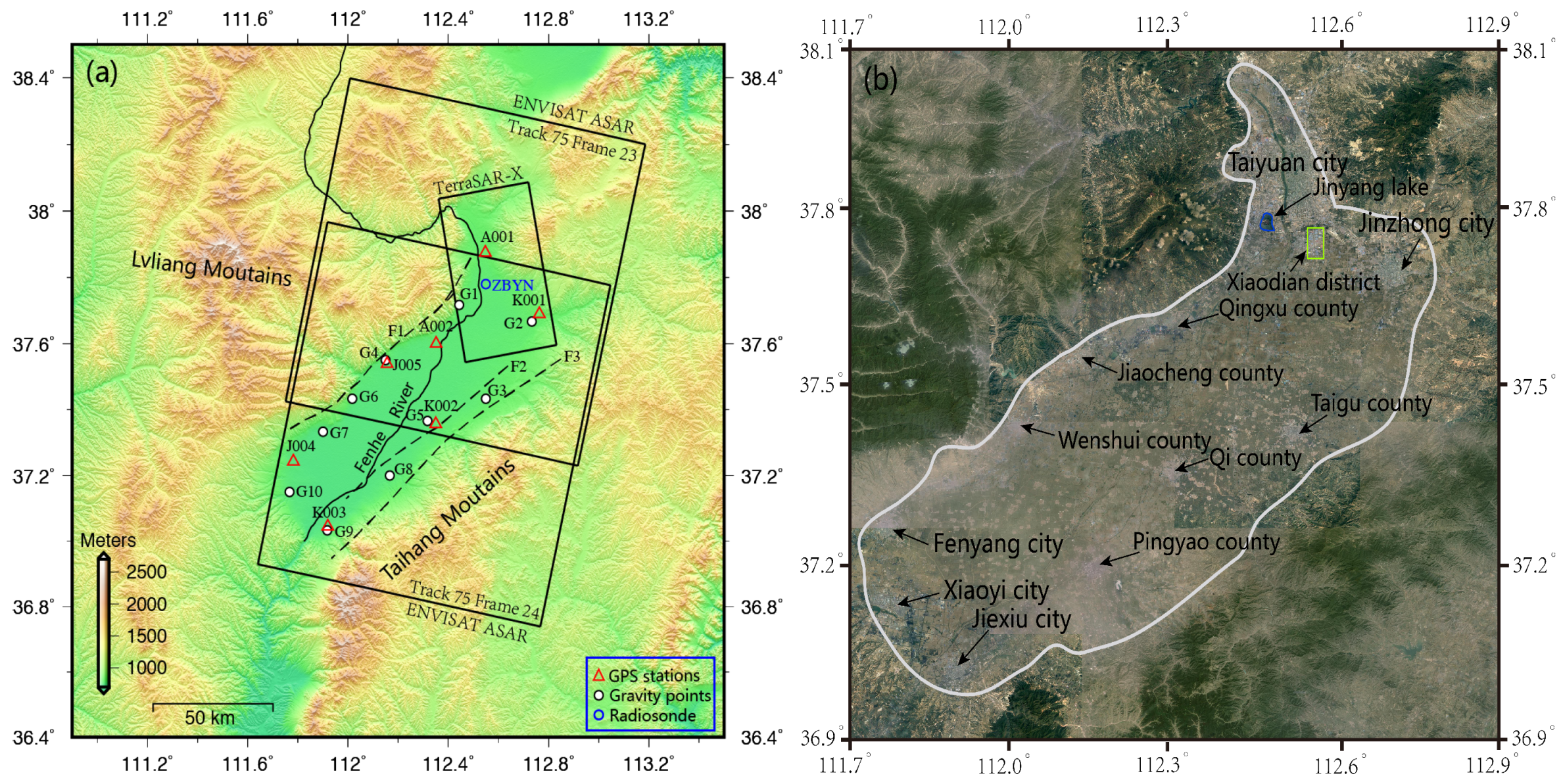
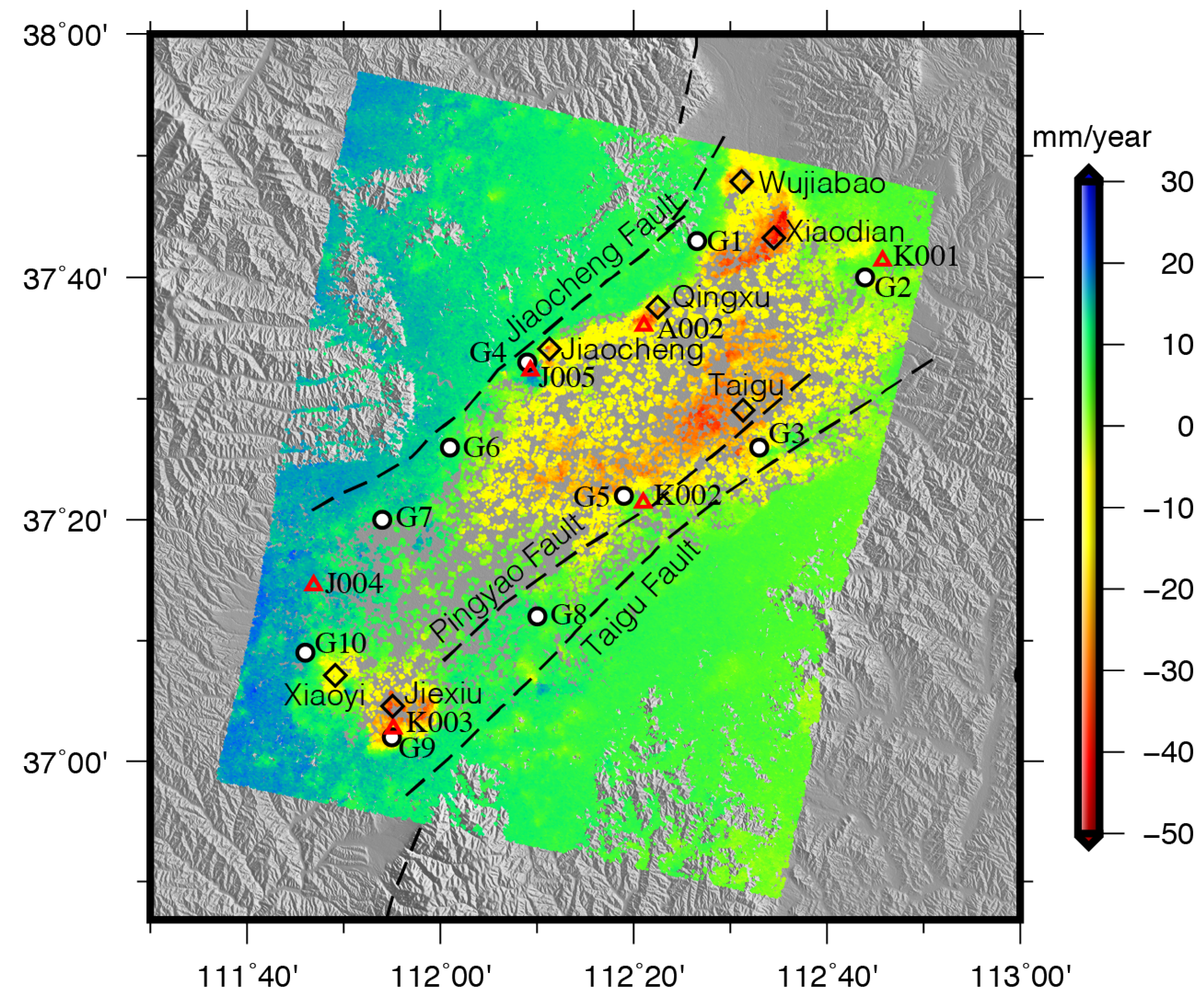
2. Study Area
3. Available Data Sets
3.1. SAR Data
3.2. Continuous GPS
3.3. Gravity Measurements
4. Methodology
4.1. Tropospheric Delay in InSAR Measurements
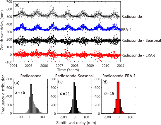
4.2. Seasonal Effects of Tropospheric Delay
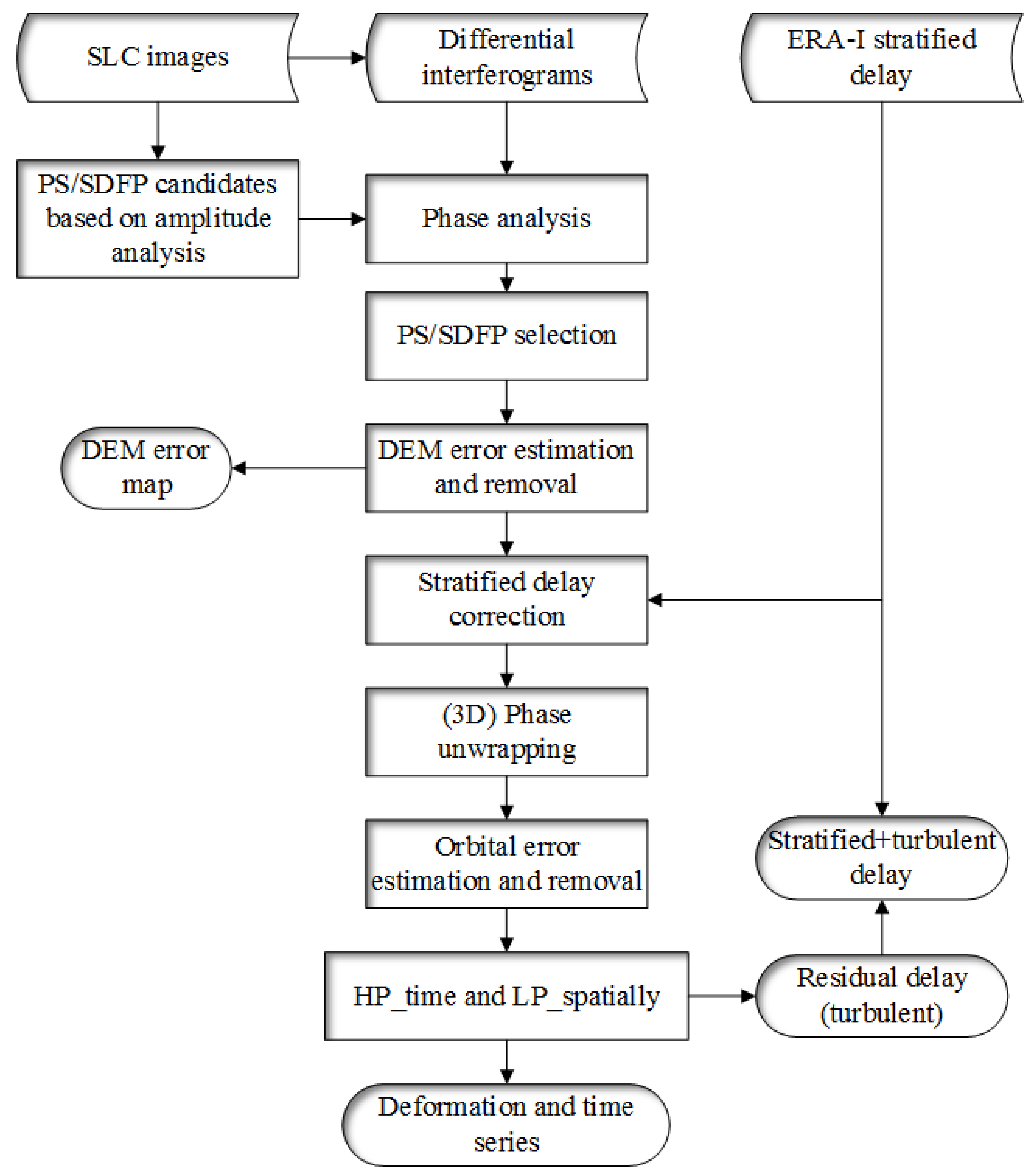
4.3. Atmosphere-Corrected Time Series InSAR
5. Results
6. Discussion
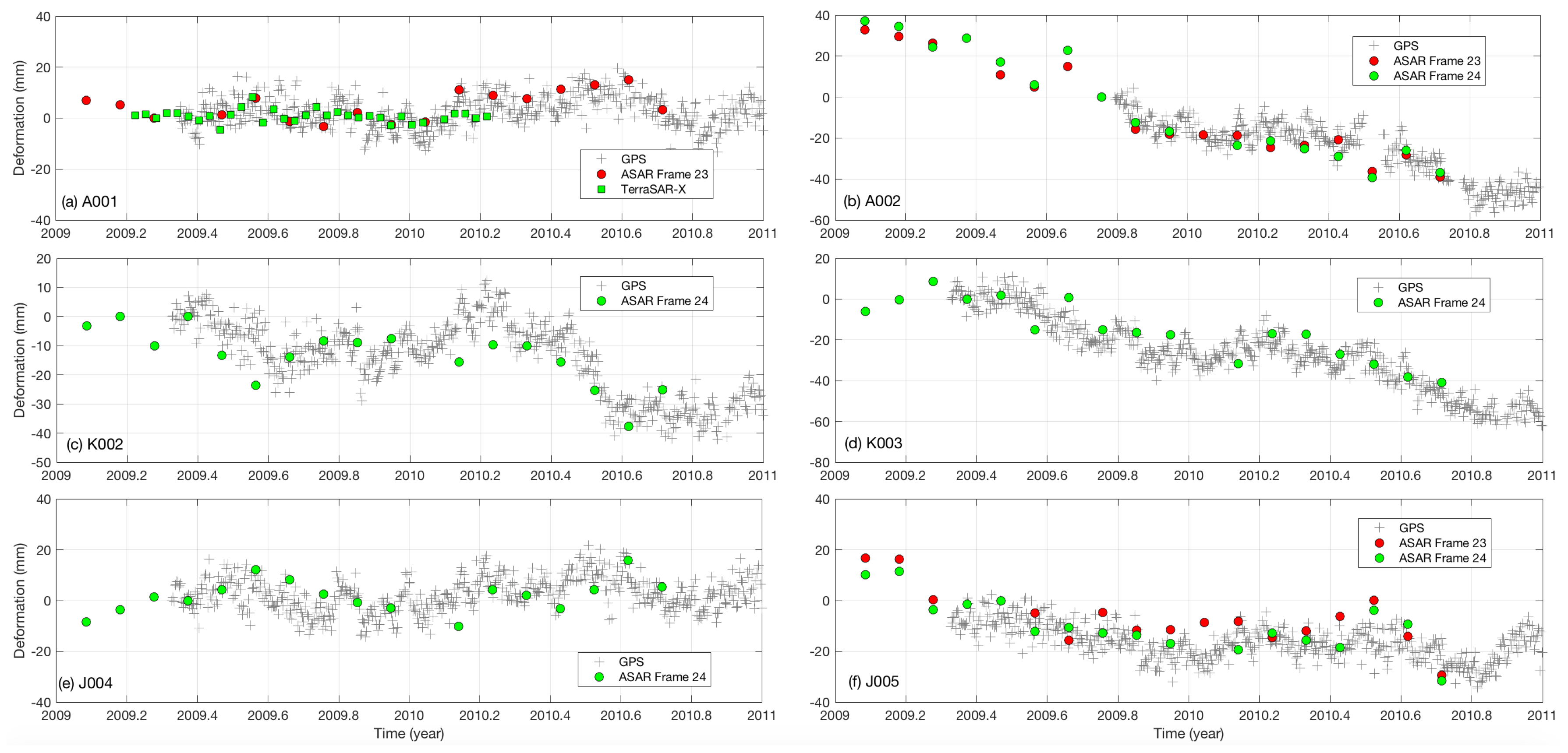
6.1. Comparison between InSAR and CGPS Observations
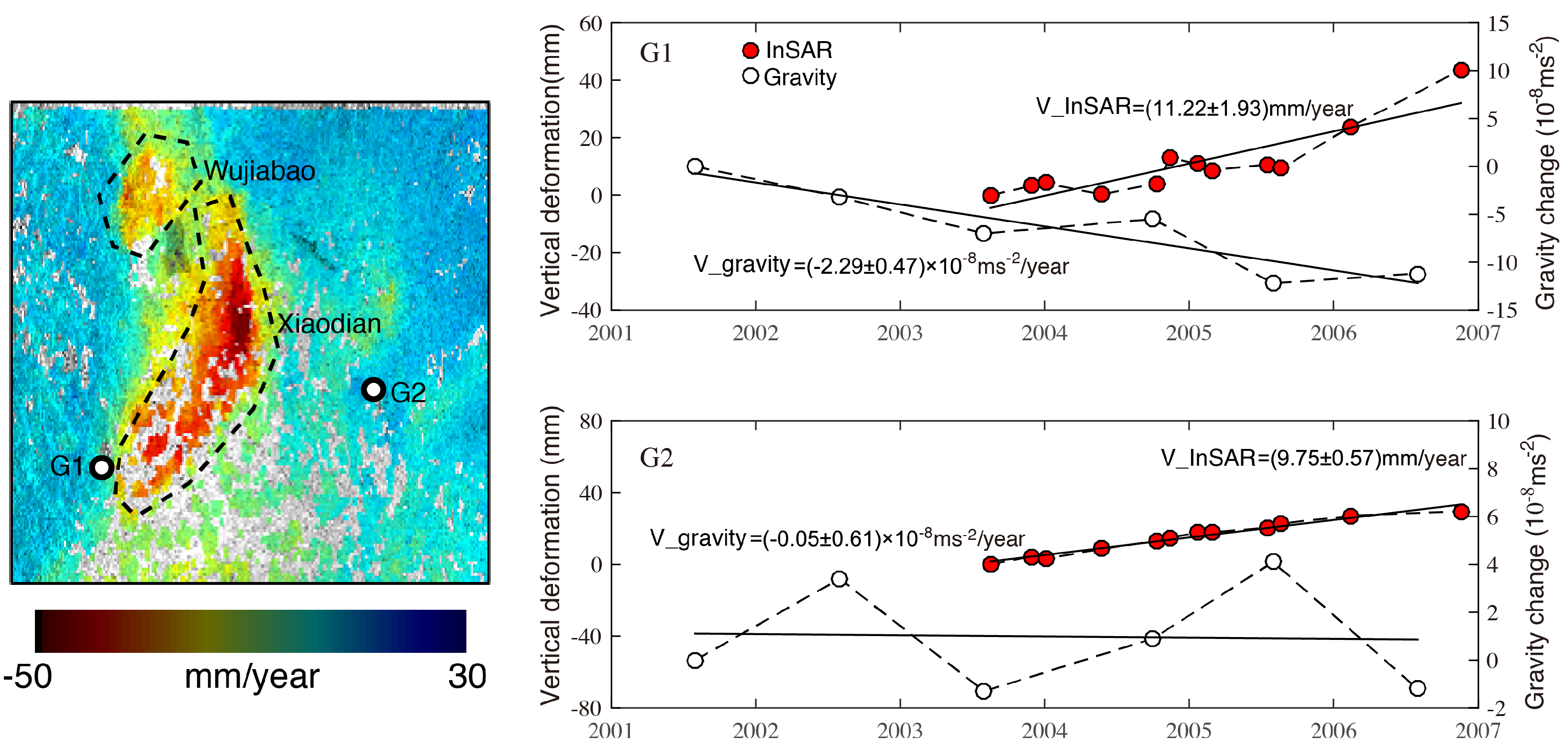
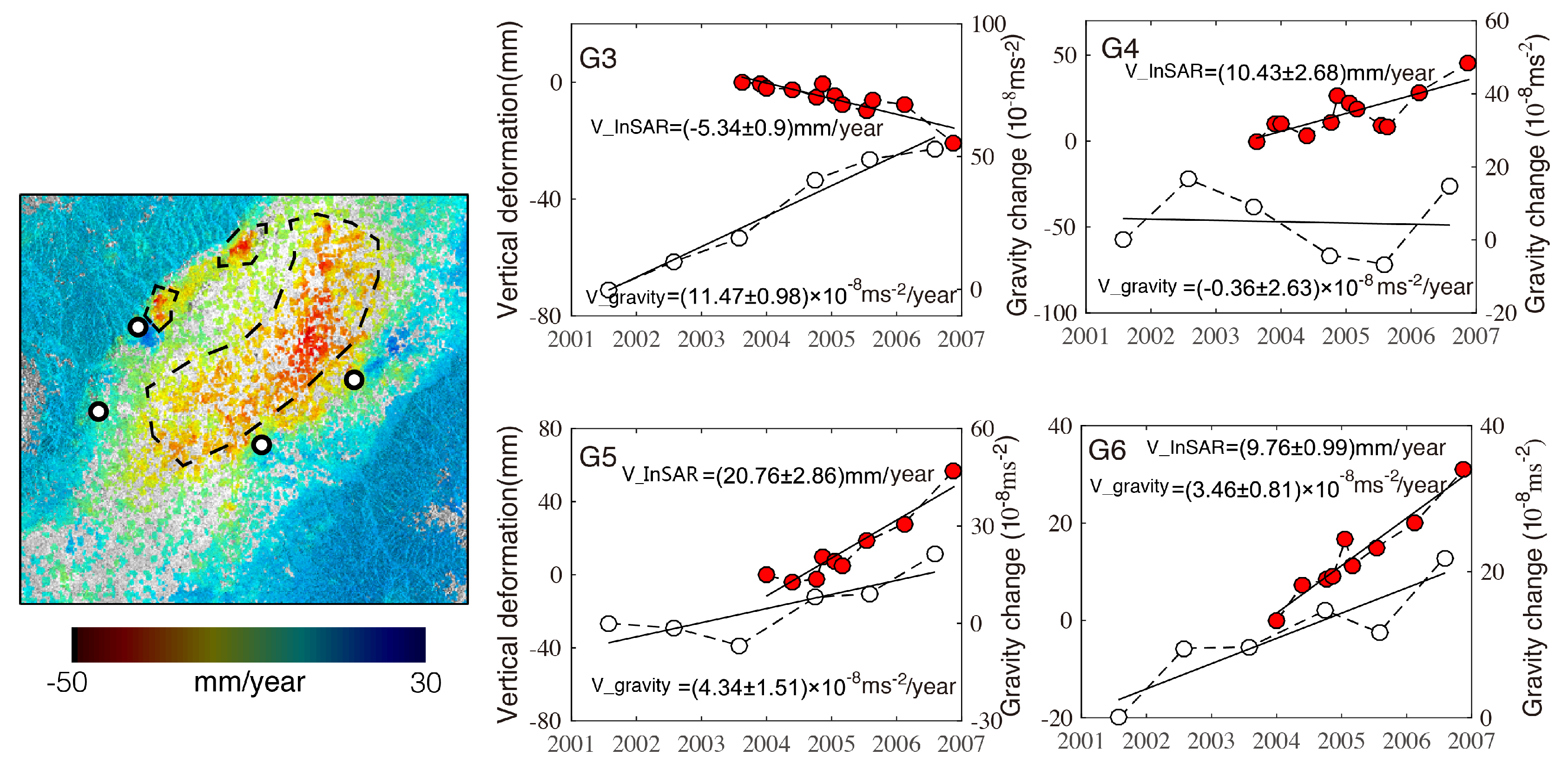
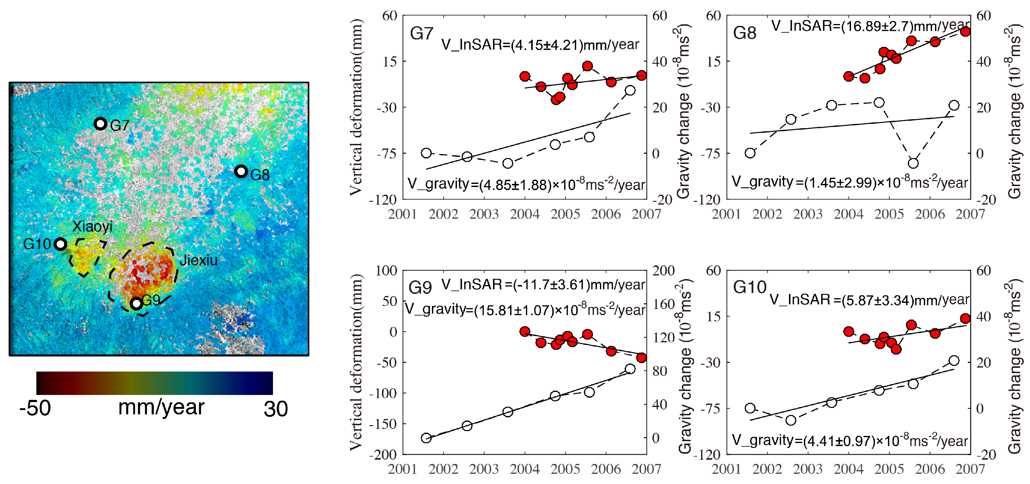
6.2. Ground Deformation and Gravity Changes
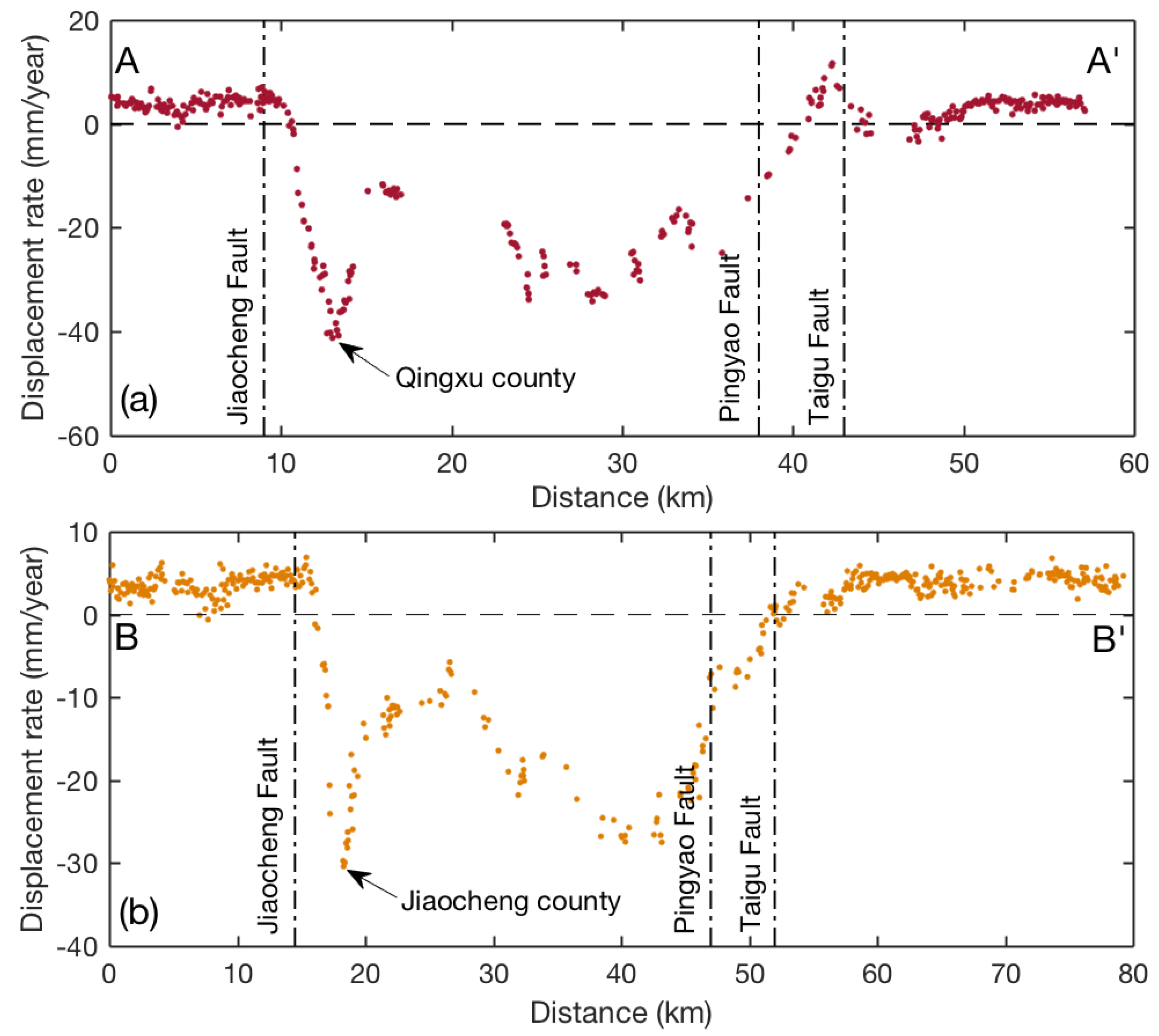
6.3. Correlation between Deformation and Pre-Existing Faults
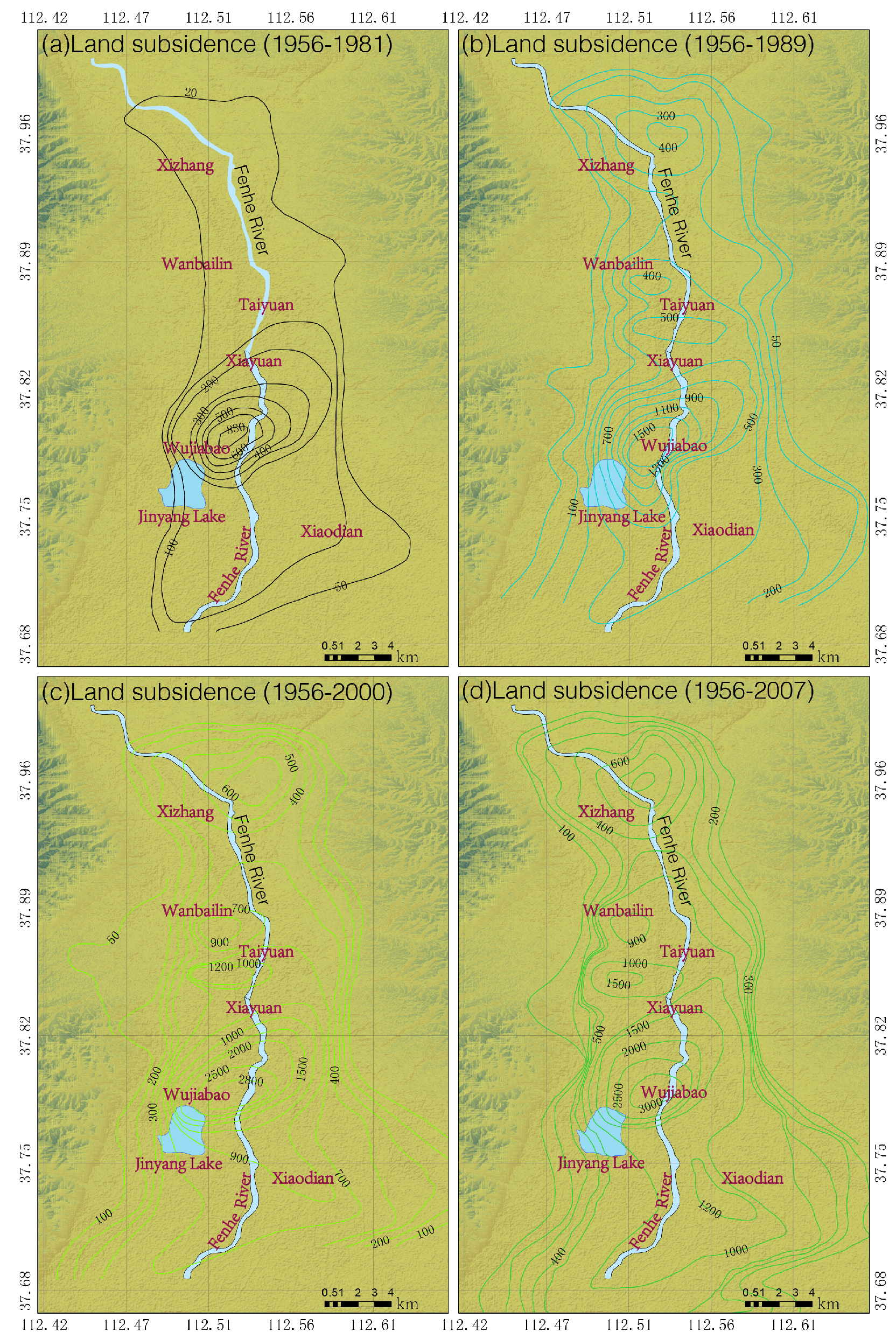
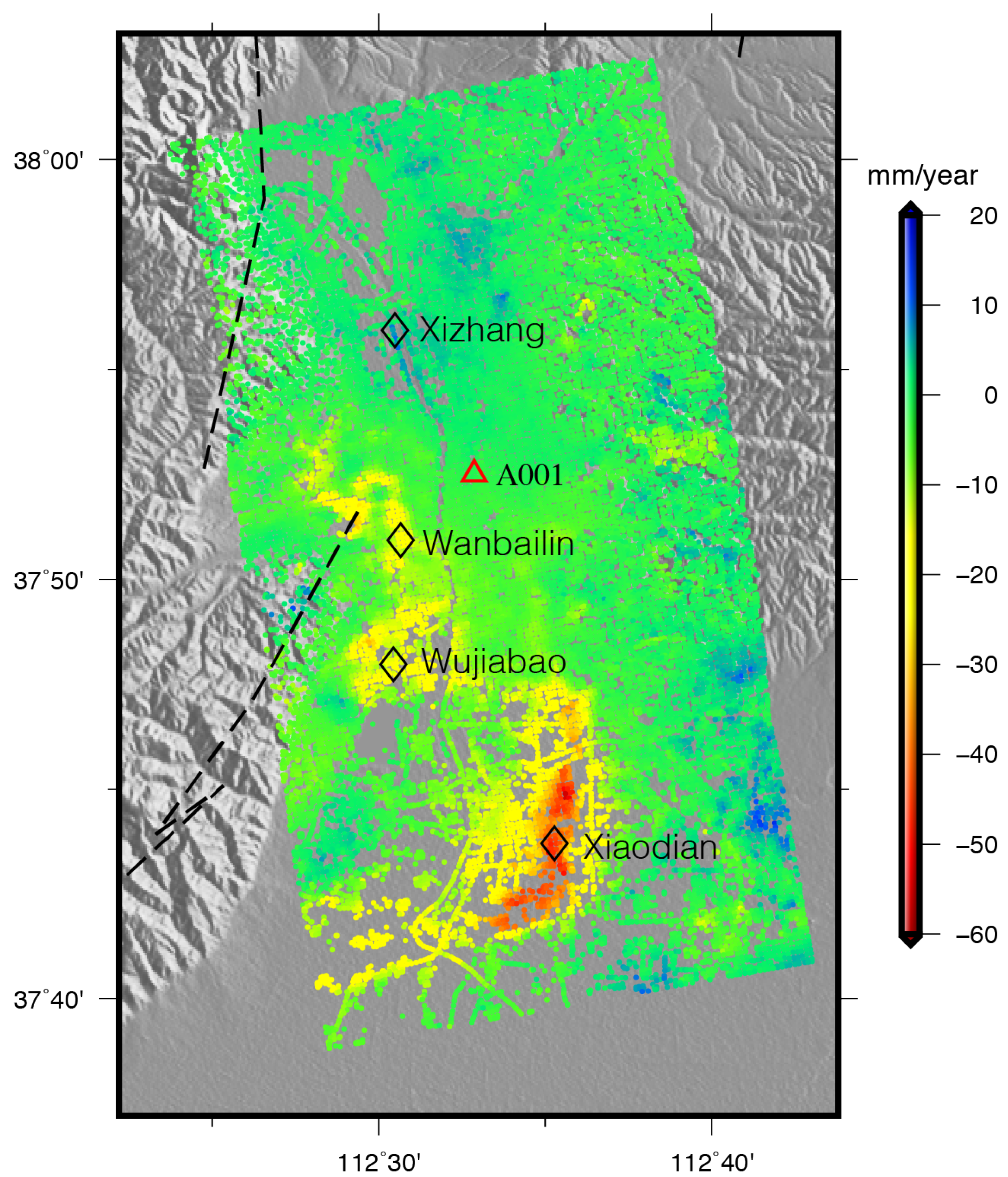
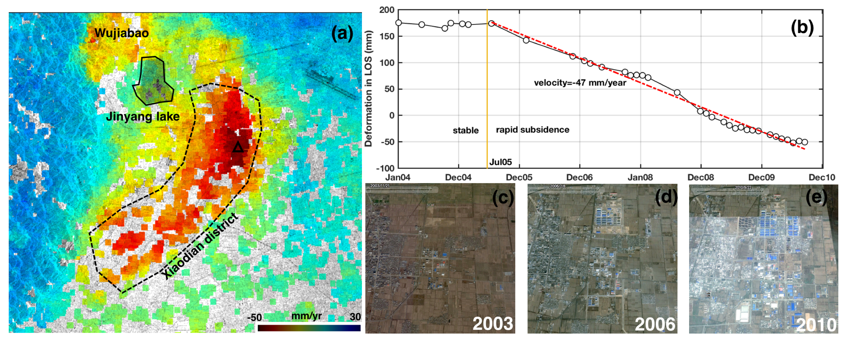
6.4. Migration of Subsidence Areas to Newly Urbanized Areas
7. Conclusions
Author Contributions
Funding
Acknowledgments
Conflicts of Interest
References
- Chaussard, E.; Wdowinski, S.; Cabral-Cano, E.; Amelung, F. Land subsidence in central Mexico detected by ALOS InSAR time-series. Remote Sens. Environ. 2014, 140, 94–106. [Google Scholar] [CrossRef]
- Motagh, M.; Walter, T.R.; Sharifi, M.A.; Fielding, E.; Schenk, A.; Anderssohn, J.; Zschau, J. Land subsidence in Iran caused by widespread water reservoir overexploitation. Geophys. Res. Lett. 2008, 35, L16403. [Google Scholar] [CrossRef]
- Motagh, M.; Shamshiri, R.; Haghshenas Haghighi, M.; Wetzel, H.-U.; Akbari, B.; Nahavandchi, H.; Roessner, S.; Arabi, S. Quantifying groundwater exploitation induced subsidence in the Rafsanjan plain, southeastern Iran, using InSAR time-series and in situ measurements. Eng. Geol. 2017, 218, 134–151. [Google Scholar] [CrossRef]
- Yang, Z.; Li, Z.; Zhu, J.; Preusse, A.; Yi, H.; Hu, J.; Feng, G.; Papst, M. Retrieving 3-D large displacements of mining areas from a single amplitude pair of SAR using offset tracking. Remote Sens. 2017, 9, 338. [Google Scholar] [CrossRef]
- Li, Z.; Zhao, R.; Hu, J.; Wen, L.; Feng, G.; Zhang, Z.; Wang, Q. InSAR analysis of surface deformation over permafrost to estimate active layer thickness based on one-dimensional heat transfer model of soils. Sci. Rep. 2015, 5, 15542. [Google Scholar] [CrossRef] [PubMed] [Green Version]
- Dang, V.K.; Doubre, C.; Weber, C.; Gourmelen, N.; Masson, F. Recent land subsidence caused by the rapid urban development in the Hanoi region (Vietnam) using ALOS InSAR data. Nat. Hazards Earth Syst. Sci. 2014, 14, 657–674. [Google Scholar] [CrossRef] [Green Version]
- Liu, Y.; Zhao, C.; Zhang, Q.; Yang, C.; Zhang, J. Land subsidence in Taiyuan, China, monitored by InSAR technique with multisensor SAR datasets from 1992 to 2015. IEEE J. Sel. Top. Appl. Earth Obs. Remote Sens. 2018, 11, 1–11. [Google Scholar] [CrossRef]
- Tang, W.; Liao, M.; Yuan, P. Atmospheric correction in time-series SAR interferometry for land surface deformation mapping—A case study of Taiyuan, China. Adv. Sp. Res. 2016, 58, 310–325. [Google Scholar] [CrossRef]
- Zhang, Q.; Zhu, W.; Ding, X.; Zhao, C.; Yang, C.; Qu, W. Two-dimensional deformation monitoring over Qingxu (China) by integrating C-, L- and X-bands SAR images. Remote Sens. Lett. 2014, 5, 27–36. [Google Scholar] [CrossRef]
- Ma, R.; Wang, Y.; Yan, C.; Ma, T. Simulation of subsidence in different compressible layers due to groundwater withdrawal in Taiyuan, Shanxi, China. In Proceedings of the Seventh International Symposium on Land Subsidence, Shanghai, China, 23–28 October 2005; pp. 744–753. [Google Scholar]
- Ma, T.; Wang, Y.; Yan, S.; Ma, R.; Yan, C.; Zhou, X. Causes of land subsidence in Taiyuan City, Shanxi, China. In Proceedings of the Seventh International Symposium on Land Subsidence, Shanghai, China, 23–28 October 2005; pp. 102–110. [Google Scholar]
- Yan, S.; Guo, Q.; Zhou, X. Design of land subsidence monitoring network: A case study at Taiyuan, Shanxi, China. In Proceedings of the Seventh International Symposium on Land Subsidence, Shanghai, China, 23–28 October 2005; pp. 460–465. [Google Scholar]
- Ferretti, A.; Savio, G.; Barzaghi, R.; Borghi, A.; Musazzi, S.; Novali, F.; Prati, C.; Rocca, F. Submillimeter Accuracy of InSAR Time Series: Experimental Validation. IEEE Trans. Geosci. Remote Sens. 2007, 45, 1142–1153. [Google Scholar] [CrossRef]
- Schmidt, D.A.; Bürgmann, R. Time-dependent land uplift and subsidence in the Santa Clara valley, California, from a large interferometric synthetic aperture radar data set. J. Geophys. Res. Solid Earth 2003, 108, 1142–1153. [Google Scholar] [CrossRef]
- Bekaert, D.P.S.; Walters, R.J.; Wright, T.J.; Hooper, A.J.; Parker, D.J. Statistical comparison of InSAR tropospheric correction techniques. Remote Sens. Environ. 2015, 170, 40–47. [Google Scholar] [CrossRef]
- Liu, Z.; Jung, H.-S.S.; Lu, Z. Joint correction of ionosphere noise and orbital error in L-band SAR interferometry of interseismic deformation in southern California. IEEE Trans. Geosci. Remote Sens. 2014, 52, 3421–3427. [Google Scholar] [CrossRef]
- Liao, H.; Meyer, F.J.; Scheuchl, B.; Mouginot, J.; Joughin, I.; Rignot, E. Ionospheric correction of InSAR data for accurate ice velocity measurement at polar regions. Remote Sens. Environ. 2018, 209, 166–180. [Google Scholar] [CrossRef]
- Lin, Y.N.; Simons, M.; Hetland, E.A.; Muse, P.; DiCaprio, C. A multiscale approach to estimating topographically correlated propagation delays in radar interferograms. Geochem. Geophys. Geosyst. 2010, 11. [Google Scholar] [CrossRef] [Green Version]
- Onn, F.; Zebker, H.A. Correction for interferometric synthetic aperture radar atmospheric phase artifacts using time series of zenith wet delay observations from a GPS network. J. Geophys. Res. 2006, 111. [Google Scholar] [CrossRef] [Green Version]
- Yu, C.; Penna, N.T.; Li, Z. Generation of real-time mode high-resolution water vapor fields from GPS observations. J. Geophys. Res. 2017, 122, 2008–2025. [Google Scholar] [CrossRef] [Green Version]
- Yu, C.; Li, Z.; Penna, N.T. Interferometric synthetic aperture radar atmospheric correction using a GPS-based iterative tropospheric decomposition model. Remote Sens. Environ. 2018, 204, 109–121. [Google Scholar] [CrossRef]
- Li, Z.H.; Muller, J.P.; Cross, P. Comparison of precipitable water vapor derived from radiosonde, GPS, and Moderate-Resolution Imaging Spectroradiometer measurements. J. Geophys. Res. 2003, 108. [Google Scholar] [CrossRef] [Green Version]
- Jolivet, R.; Agram, P.S.; Lin, N.Y.; Simons, M.; Doin, M.; Peltzer, G.; Li, Z. Improving InSAR geodesy using Global Atmospheric Models. J. Geophys. Res. Solid Earth 2014, 119, 2324–2341. [Google Scholar] [CrossRef] [Green Version]
- Berardino, P.; Fornaro, G.; Lanari, R.; Sansosti, E. A new algorithm for surface deformation monitoring based on small baseline differential SAR interferograms. IEEE Trans. Geosci. Remote Sens. 2002, 10, 40. [Google Scholar] [CrossRef]
- Ferretti, A.; Prati, C.; Rocca, F. Permanent scatters in SAR interferometry. IEEE Trans. Geosci. Remote Sens. 2001, 39, 8–20. [Google Scholar] [CrossRef]
- Hooper, A.; Segall, P.; Zebker, H. Persistent scatterer interferometric synthetic aperture radar for crustal deformation analysis, with application to Volcán Alcedo, Galápagos. J. Geophys. Res. Solid Earth 2007, 112, 1–21. [Google Scholar] [CrossRef]
- Fattahi, H.; Amelung, F. InSAR bias and uncertainty due to the systematic and stochastic tropospheric delay. J. Geophys. Res. Solid Earth 2015, 120, 8758–8773. [Google Scholar] [CrossRef] [Green Version]
- Tang, Q.; Xu, Q.; Zhang, F.; Huang, Y.; Liu, J.; Wang, X.; Yang, Y.; Liu, X. Geochemistry of iodine-rich groundwater in the Taiyuan Basin of central Shanxi Province, North China. J. Geochem. Explor. 2013, 135, 117–123. [Google Scholar] [CrossRef]
- Shamshiri, R.; Motagh, M.; Baes, M.; Sharifi, M.A. Deformation analysis of the Lake Urmia causeway (LUC) embankments in northwest Iran: Insights from multi-sensor interferometry synthetic aperture radar (InSAR) data and finite element modeling (FEM). J. Geod. 2014, 12, 1171–1185. [Google Scholar] [CrossRef]
- Emadali, L.; Motagh, M.; Haghighi, M.H. Characterizing post-construction settlement of the Masjed-Soleyman embankment dam, Southwest Iran, using TerraSAR-X SpotLight radar imagery. Eng. Struct. 2017, 143, 261–273. [Google Scholar] [CrossRef] [Green Version]
- Yuan, P.; Sun, H.; Qin, C.; Zhang, L. Analysis of Anhui CORS reference stations 3D velocity field. Geomatics Inf. Sci. Wuhan Univ. 2016, 41, 535–540. [Google Scholar] [CrossRef]
- Xuan, S.; Shen, C.; Xing, L.; Li, H. Gravity change and subsidence of Tiyuan Basin. J. Geod. Geodyn. 2014, 34, 24–27. [Google Scholar] [CrossRef]
- Ramon, H. Radar Interferometry: Data Interpretation and Error Analysis, 1st ed.; Springer: Delft, The Netherlands, 2001; pp. 70–72. ISBN 90-73235-43-X. [Google Scholar]
- Hooper, A.; Bekaert, D.; Spaans, K.; Arıkan, M. Recent advances in SAR interferometry time series analysis for measuring crustal deformation. Tectonophysics 2012, 514, 1–13. [Google Scholar] [CrossRef]
- Jung, J.; Kim, D.; Park, S. Correction of atmospheric phase screen in time series InSAR using WRF model for monitoring volcanic activities. IEEE Trans. Geosci. Remote Sens. 2014, 52, 2678–2689. [Google Scholar] [CrossRef]
- Zhu, W.; Zhang, Q.; Ding, X.; Zhao, C.; Yang, C.; Qu, W. Recent ground deformation of Taiyuan basin (China) investigated with C-, L-, and X-bands SAR images. J. Geodyn. 2013, 70, 28–35. [Google Scholar] [CrossRef]
- Imanishi, Y.; Sato, T.; Higashi, T.; Sun, W.; Okubo, S. A network of superconducting gravimeters detects submicrogal coseismic gravity changes. Science 2004, 306, 476–478. [Google Scholar] [CrossRef] [PubMed]
- Bagnardi, M.; Poland, M.P.; Carbone, D.; Baker, S.; Battaglia, M.; Amelung, F. Gravity changes and deformation at Kīlauea Volcano, Hawaii, associated with summit eruptive activity, 2009–2012. J. Geophys. Res. Solid Earth 2014, 119, 7288–7305. [Google Scholar] [CrossRef]
- Hwang, C.; Cheng, T.; Cheng, C.C.; Hung, W.C. Land subsidence using absolute and relative gravimetry: A case study in central Taiwan. Surv. Rev. 2016, 42, 27–39. [Google Scholar] [CrossRef]
- Chen, Y. Study on the characteristics of ground fissures in Shanxi fault basin. Chin. J. Geol. Hazards Control 2016, 27, 72–80. [Google Scholar] [CrossRef]
- Sun, X.; Peng, J.; Cui, X.; Jiang, Z. Relationship between ground fissures, groundwater exploration and land subsidence in Taiyuan basin. Chin. J. Geol. Hazards Control 2016, 27, 91–98. [Google Scholar] [CrossRef]
- Caine, J.S.; Evans, J.P.; Forster, C.B. Fault zone architechture and permeability structure. Geology 1996, 24, 1025–1028. [Google Scholar] [CrossRef]
- Teufel, L.W. Permeability changes during shear deformation of fractured rock. In Proceedings of the 28th U.S. Symposium on Rock Mechanics (USRMS), Tucson, AZ, USA, 29 June–1 July 1987; pp. 473–480. [Google Scholar]
- Hu, R.L.; Yue, Z.Q.; Wang, L.C.; Wang, S.J. Review on current status and challenging issues of land subsidence in China. Eng. Geol. 2004, 76, 65–77. [Google Scholar] [CrossRef]


| SAR Sensor | Track, Frame | Time Span | Orbit Mode | (Degree) | N | M |
|---|---|---|---|---|---|---|
| ENVISAT ASAR | T75, F23 | 20030817-20100919 | descending | 23 | 39 | 181 |
| ENVISAT ASAR | T75, F24 | 20040104-20100919 | descending | 23 | 36 | 186 |
| TerraSAR-X | - | 20090321-20100323 | ascending | 30 | 33 | 32 |
| GPS Station | Longitude | Latitude | North | East | Up |
|---|---|---|---|---|---|
| A001 | 112.5 | 37.9 | −11.53 ± 0.09 | 31.36 ± 0.09 | 3.42 ± 0.48 |
| A002 | 112.4 | 37.6 | −9.17 ± 0.17 | 28.9 ± 0.15 | −35.84 ± 0.81 |
| K001 | 112.7 | 37.7 | −13.64 ± 0.10 | 33.31 ± 0.09 | 0.95 ± 0.43 |
| K002 | 112.4 | 37.4 | −10.85 ± 0.09 | 32.30 ± 0.09 | −15.72 ± 0.52 |
| K003 | 111.9 | 37.0 | −8.34 ± 0.09 | 34.22 ± 0.09 | −29.81 ± 0.46 |
| J004 | 111.8 | 37.2 | −9.41 ± 0.10 | 31.77 ± 0.09 | 4.91 ± 0.48 |
| J005 | 112.2 | 37.5 | −10.68 ± 0.10 | 37.63 ± 0.11 | −5.98 ± 0.47 |
| Station | Aug 2001 | Aug 2002 | Aug 2003 | Oct 2004 | Aug 2005 | Aug 2006 |
|---|---|---|---|---|---|---|
| G1 | −9.9945 | −9.9977 | −10.0015 | −10.0000 | −10.0067 | −10.0057 |
| G2 | −12.1628 | −12.1594 | −12.1641 | −12.1619 | −12.1587 | −12.1640 |
| G3 | −42.0322 | −42.0217 | −42.0130 | −41.9909 | −41.9833 | −41.9793 |
| G4 | −23.8529 | −23.8363 | −23.8437 | −23.8571 | −23.8595 | −23.8382 |
| G5 | −32.5414 | −32.5428 | −32.5482 | −32.5334 | −32.5322 | −32.5202 |
| G6 | −30.7725 | −30.7630 | −30.7628 | −30.7578 | −30.7608 | −30.7506 |
| G7 | −44.4278 | −44.4295 | −44.4323 | −44.4239 | −44.4206 | −44.4004 |
| G8 | −53.5224 | −53.5077 | −53.5015 | −53.5002 | −53.5266 | −53.5017 |
| G9 | −57.0167 | −57.0028 | −56.9864 | −56.9667 | −56.9620 | −56.9340 |
| G10 | −49.1414 | −49.1466 | −49.1387 | −49.1337 | −49.1309 | −49.1207 |
| CGPS | GPS | ASAR Frame 23 | ASAR Frame 24 | TerraSAR-X | |||
|---|---|---|---|---|---|---|---|
| V | (2009.084-2010.715) | (2009.084-2010.715) | (2009.216-2010.221) | ||||
| A001 | 1.3 | 5.7 | 4.1 | - | - | 1.3 | 1.1 |
| 2009.349-2010.998 | |||||||
| A002 | −21.3 | −17.7 | −22.9 | −24.5 | −21.7 | - | - |
| 2009.793-2010.995 | |||||||
| K002 | −16.4 | - | - | −13.2 | −17.0 | - | - |
| 2009.327-2010.998 | |||||||
| K003 | −30.3 | - | - | −29.4 | −30.2 | - | - |
| 2009.327-2010.998 | |||||||
| J004 | 2.3 | - | - | 0.9 | 1.1 | - | - |
| 2009.327-2010.998 | |||||||
| J005 | −7.0 | - | - | −10.6 | −9.9 | - | - |
| 2009.327-2010.998 | |||||||
| Subsidence Centers | 1956–1981 | 1981–1989 | 1989–2000 | 2003–2008 | 2009–2010 |
|---|---|---|---|---|---|
| Xizhang | −3.0 | −43.4 | −25.0 | +2.3 | +2.5 |
| Wanbailin | −2.5 | −46.8 | −46.7 | −20.5 | −12.6 |
| Xiayuan | −3.6 | −55.3 | −86.0 | −22.5 | −15.4 |
| Wujiabao | −33.1 | −114.0 | −96.2 | −28.9 | −30.9 |
| Xiaodian | no subsidence | no subsidence | no subsidence | −27.9 | −50.8 |
© 2018 by the authors. Licensee MDPI, Basel, Switzerland. This article is an open access article distributed under the terms and conditions of the Creative Commons Attribution (CC BY) license (http://creativecommons.org/licenses/by/4.0/).
Share and Cite
Tang, W.; Yuan, P.; Liao, M.; Balz, T. Investigation of Ground Deformation in Taiyuan Basin, China from 2003 to 2010, with Atmosphere-Corrected Time Series InSAR. Remote Sens. 2018, 10, 1499. https://0-doi-org.brum.beds.ac.uk/10.3390/rs10091499
Tang W, Yuan P, Liao M, Balz T. Investigation of Ground Deformation in Taiyuan Basin, China from 2003 to 2010, with Atmosphere-Corrected Time Series InSAR. Remote Sensing. 2018; 10(9):1499. https://0-doi-org.brum.beds.ac.uk/10.3390/rs10091499
Chicago/Turabian StyleTang, Wei, Peng Yuan, Mingsheng Liao, and Timo Balz. 2018. "Investigation of Ground Deformation in Taiyuan Basin, China from 2003 to 2010, with Atmosphere-Corrected Time Series InSAR" Remote Sensing 10, no. 9: 1499. https://0-doi-org.brum.beds.ac.uk/10.3390/rs10091499