Validation of Hourly Global Horizontal Irradiance for Two Satellite-Derived Datasets in Northeast Iraq

Abstract

Several sectors need global horizontal irradiance (GHI) data for various purposes. However, the availability of a long-term time series of high quality in situ GHI measurements is limited. Therefore, several studies have tried to estimate GHI by re-analysing climate data or satellite images. Validation is essential for the later use of GHI data in the regions with a scarcity of ground-recorded data. This study contributes to previous studies that have been carried out in the past to validate HelioClim-3 version 5 (HC3v5) and the Copernicus Atmosphere Monitoring Service, using radiation service version 3 (CRSv3) data of hourly GHI from satellite-derived datasets (SDD) with nine ground stations in northeast Iraq, which have not been used previously. The validation is carried out with station data at the pixel locations and two other data points in the vicinity of each station, which is something that is rarely seen in the literature. The temporal and spatial trends of the ground data are well captured by the two SDDs. Correlation ranges from 0.94 to 0.97 in all-sky and clear-sky conditions in most cases, while for cloudy-sky conditions, it is between 0.51–0.72 and 0.82–0.89 for the clearness index. The bias is negative for most of the cases, except for three positive cases. It ranges from −7% to 4%, and −8% to 3% for the all-sky and clear-sky conditions, respectively. For cloudy-sky conditions, the bias is positive, and differs from one station to another, from 16% to 85%. The root mean square error (RMSE) ranges between 12–20% and 8–12% for all-sky and clear-sky conditions, respectively. In contrast, the RMSE range is significantly higher in cloudy-sky conditions: above 56%. The bias and RMSE for the clearness index are nearly the same as those for the GHI for all-sky conditions. The spatial variability of hourly GHI SDD differs only by 2%, depending on the station location compared to the data points around each station. The variability of two SDDs is quite similar to the ground data, based on the mean and standard deviation of hourly GHI in a month. Having station data at different timescales and the small number of stations with GHI records in the region are the main limitations of this analysis.

1. Introduction

Global horizontal irradiance (GHI), both in the atmosphere and on the earth’s surface, is a crucial parameter in the fields of atmosphere interaction, solar energy, architecture, and agriculture. High-resolution GHI data are required for studying those fields. Therefore, several studies have tried to estimate solar radiation (SR) and its components from either ground measurements or satellite images using several models [1,2,3,4,5,6]. The ground measurements of GHI have high accuracy and high temporal availability, whereas the high spatial resolution of recorded data and the number of stations with SR data are limited in most geographical areas. The reasons are the purchase and high maintenance costs of pyranometers. Satellite images have been analysed to estimate GHI in order to cover the scarcity of ground measurement data. Most of the affordable satellite images for that purpose are the geostationary satellite images, namely Meteosat First Generation (MFG) and Meteosat Second Generation (MSG)/Spinning Enhanced Visible and Infrared Imager (SEVIRI), The Japanese Geostationary Meteorological Satellite (GMS), and the Geostationary Operational Environmental Satellite system (GOES) [7]. Hence, others such as the Moderate Resolution Imaging Spectroradiometer (MODIS) [8] and Landsat images have been used [9], but their temporal resolution is not acceptable.

The basic idea of estimating GHI from satellite images is to find the relationship between satellite images and ground measurements, either with statistical or physical approaches [10]. The popular method of Heliosat-2 (H2), which is based on developing Heliosat-1 to be more physical than empirical, can be, applied to large time-series data of meteorological satellites. The H2 principle is that the radiance of a cloud pixel is high in the visible band. It tests the difference of the reflectance between the cloud pixel and the clear-sky pixel; this is called a cloud index. This data and the data of the Linke turbidity factor are used to measure GHI [11]. The H2 has been developed by changing some inputs to the model in several studies [12,13,14]. Other studies also used satellite imagery with different techniques for GHI estimations [15,16,17].

There are several satellite-derived datasets (SDDs) for establishing, measuring, modelling and estimating GHI, which can be found in [18,19]. An SDD from MSG has been used to create a solar map [20]. Studies which merged ground data with the SDD for the same above purpose reveal that the merging technique for producing a solar map is better than interpolating ground data [21,22]. SDDs have also been combined with meteorological data to calibrate a GHI model [23]. The same data combinations have also been analysed to create GHI datasets for crop modelling over Europe [24]. SDDs have been utilised to assess long-term trends of a GHI time series [25]. SDDs are quite useful because of the limitations of ground data for GHI applications.

SDDs are necessary for many fields because they provide GHI for many areas and countries. Therefore, the validation of SDDs is crucial to investigate their reliability by using various methods in different geographical and climate areas, and several prior studies achieved that. For instance, the Satellite Application Facility on Climate Monitoring (CM SAF) dataset based on predicting GHI from MFG and MSG has been validated with the ground data at several stations in Europe in the period 1983–1985 [26]. The data from the same dataset with the H2 method for converting satellite images to GHI and others (SolarGis and Solemi) have also been validated in 22 cities in Europe [27]. Similarly, the CM SAF dataset of GHI has been compared against ground data at 20 stations in Sweden and Norway, and the result reveals good agreement with an accuracy of 15 W/m², corresponding to an error of roughly 8% [28]. In addition, GHI retrievals from different CM SAF products have been validated against ground measurements at eight sites in Europe, under various sky conditions. [29]. More broadly, Zhang et al. [19] have evaluated the result of the six re-analysed datasets for obtaining GHI with the ground data from measurement networks such as the Baseline Surface Radiation Network (BSRN) and others for 674 cities around the globe, with an overall bias found to be from 11–50 W/m². Hence, they used a large volume of data in various climate regions and countries; however, the results are shown according to the datasets and measurement networks, rather than for each station. This is useful for comparison between the SDDs and measurement networks, but it does not reflect a real situation for the individual stations. Moradi et al. [30] also estimated daily GHI with the H2 method in Iran, evaluating the result of the model with four stations in the country, which revealed a good agreement with 12% RMSE and 2% bias. Schillings et al. [31] validated direct normal irradiance (DNI) data at weather stations in eight cities in Saudi Arabia with Meteosat-7 data using the H2 method. The results indicate a good agreement with a mean bias of 4.3% from hourly data. Similarly, AL-Jumaily et al. [32] evaluated the GHI data of two Iraqi weather stations with the same method usingMeteosat-8 data for the year 2005. Positive biases of 0.024 KWh/m² and 0.012 KWh/m² GHI for daily mean values were found for both cities. The authors indicate that further research comparing Meteosat-8 data with other areas of Iraq is needed. It is necessary for studies to validate more than one SDD for comparison between them, and then select the most accurate one. Recently, GHI data from the MFG and MSG have been evaluated over India, which show an overestimation bias of 10–20% of daily mean [33]. Some other studies have evaluated SDDs over the United States in different climate regions against several ground-based measurements [34,35,36,37].

The most popular SDD is that arranged by the Solar Radiation Data (SoDa) portal [38], which contains several projects; one of them is HelioClim-3 version 4 and version 5 (HC3v4-5), which are based on the H2 method for converting satellite images of MSG to GHI. Another is the Copernicus Atmosphere Monitoring Service (CAMS) Radiation Service (CRS), which is based on Heliosat-4 (H4) for the same purpose.

Those SDDs have been validated by several studies in various areas. For example, Thomas et al. [39] have validated the hourly GHI from SDDs such as HC3v4-5 and CRS for 42 stations in Brazil. The result reveals a high correlation (an average of 96%) between HC3v4-5 and ground measurements, whereas that with CRS is lower by 2%. Similarly, r values above 0.92 for 15 min and 0.98 for daily GHI with a bias of roughly 5% were found when comparing HC3v4-5 and CRS to ground data at 14 stations over the world [40]. Hourly GHI and DNI from HC3v4-5 for all-sky conditions, and using the McClear dataset for clear-sky conditions, have been validated with ground data in seven stations over Egypt, with RMSE ranges from 6–22% [41]. Marchand et al. [42] have validated hourly GHI from HC3v4-5 and CRS with ground data at five stations in United Arab Emirates and Oman. The overall validation result is nearly 15% of the RMSE on average.

This study aims to validate the hourly GHI from HC3v5 and CRSv3 against ground measurements at nine stations in the northeast of Iraq, being the first study validating those SDDs in that region. One objective of this study is to evaluate the spatial-temporal performance of those datasets in all-sky, clear-sky, and cloudy-sky conditions and with the clearness index. Another objective is to use a new approach for validation, which is limited in the literature, comparing the GHI from ground measurements at a station against the GHI from SDDs at each station location and the two points around it, at a spatial resolution of 5 km (corresponding to that of MSG imagery), and with each point collected from a different pixel.

The study is organised as follows. The study location, ground data and SDDs are described in Section 2. The validation results are shown in Section 3. The discussion is set out in Section 4, and finally a conclusion is provided.

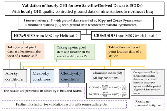
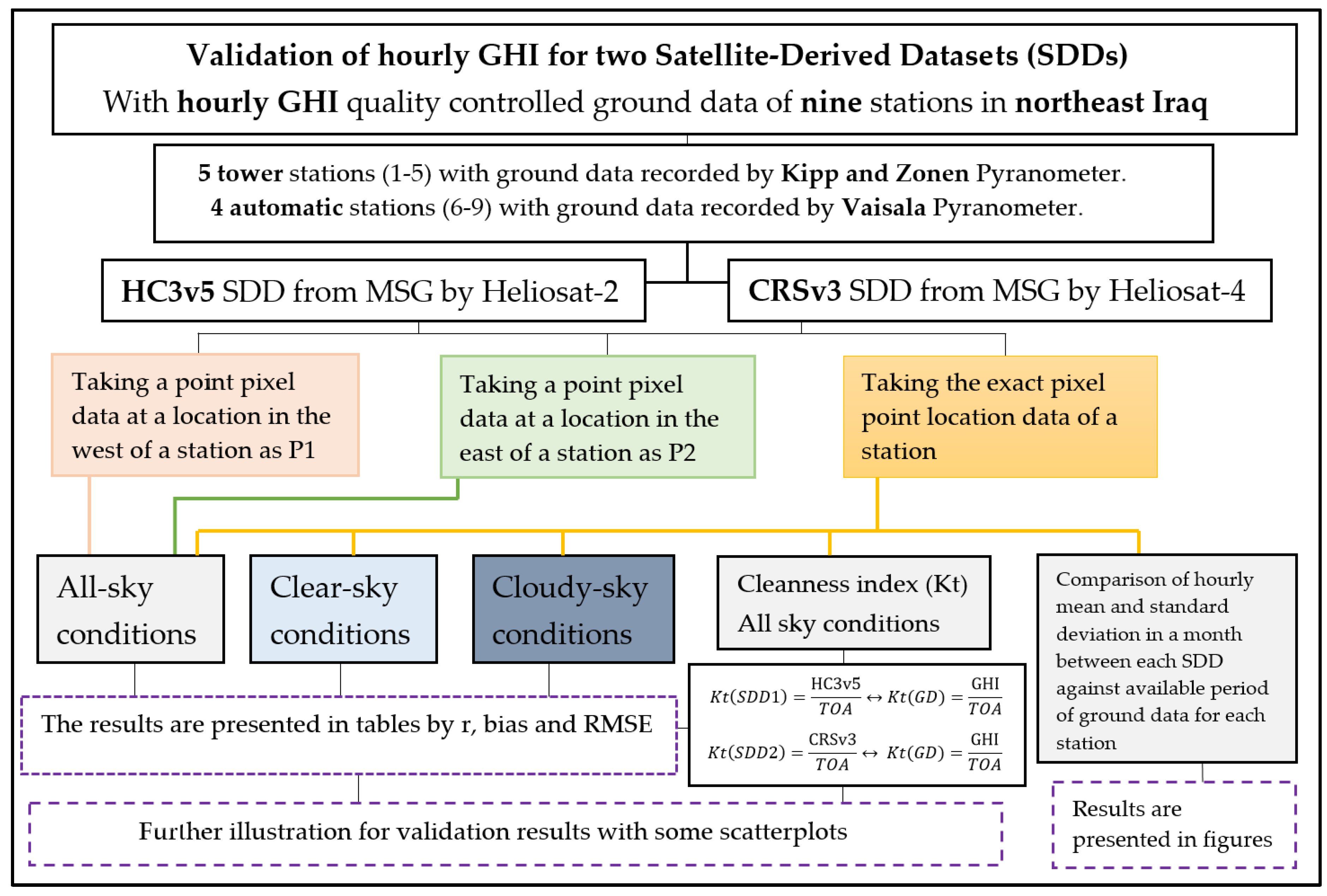
2. Materials and Methods

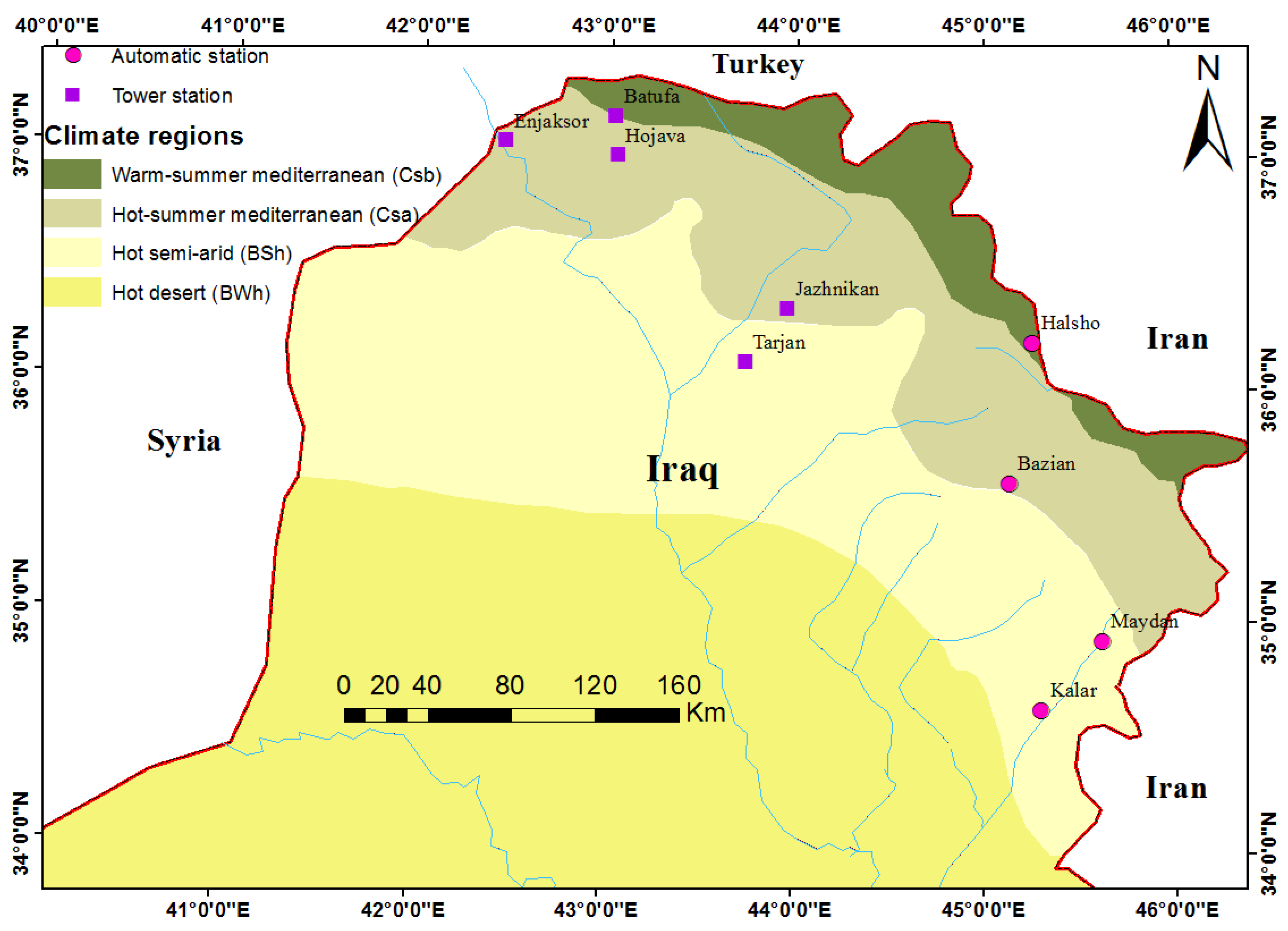
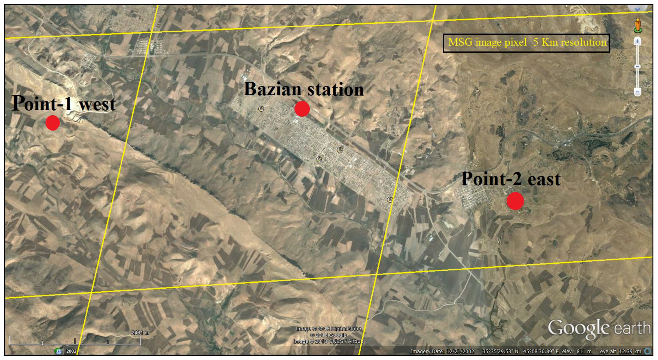
2.1. Study Site and Ground Data

The study area is located in the northeast of Iraq (latitudes [34°08′20″–37°22′36″], and longitudes [42°32′00″–46°14′29″]). It has a complex topography (mountains, hills and plain areas). According to the Koppen classification [43], two climate regions are seen in the region, which are the Mediterranean Sea and semi-arid climates (Figure 1).

The hourly GHI data with some other climate parameters were collected from two station types. First, the data are from tower stations. The pyranometer used for recording data in these stations is the Kipp and Zonen CMP6 Pyranometer. The data were collected for the period 2011–2014 from five stations, which lacked some years, from the Ministry of Electricity-Kurdistan Regional Government (KRG) (

Table 1. Tower stations with hourly GHI from Kipp and Zonen CMP6 Pyranometer.

Station	Coordinates (Degrees)		Elevation a.s.l (m)	Period
Batufa	37.1764 N	43.0236 E	947	01/01/2011–31/12/2013
P1-Batufa	37.1952 N	42.9478 E	854
P2-Batufa	37.1689 N	43.1042 E	885
Enjaksor	37.0603 N	42.4353 E	509	01/01/2011–31/12/2014
P1-Enjaksor	37.0642 N	42.3544 E	433
P2-Enjaksor	37.0533 N	42.4936 E	520
Hojava	37.0075 N	43.0369 E	933	01/01/2011–31/12/2013
P1-Hojava	37.0331 N	42.9803 E	856
P2-Hojava	37.0061 N	43.0883 E	940
Jazhnikan	36.3564 N	43.9556 E	430	01/01/2011–31/10/2013
P1-Jazhnikan	36.3672 N	43.8936 E	376
P2-Jazhnikan	36.3347 N	44.0294 E	467
Tarjan	36.1258 N	43.7353 E	276	01/01/2011–31/12/2013
P1W-Tarjan	36.1297 N	43.6686 E	263
P2-Tarjan	36.1208 N	43.7931 E	308

Note: The periods in the table are available for the ground measurements; the SDDs for the same periods have been collected for each station location and points around the stations, which were used for validation.

). Others are automatic stations equipped with an Vaisala QMS101 Pyranometer. The data were collected from the General Directorate of Meteorology and Seismology-KRG from four stations (2013–2016), which lacked some years (

Table 2. Automatic stations with hourly GHI Vaisala QMS101 Pyranometer.

Station	Coordinates (Degrees)		Elevation a.s.l (m)	Period
Halsho	36.2097 N	45.2598 E	1105	01/01/2013–31/12/2016
P1-Halsho	36.2201 N	45.2235 E	1119
P2-Halsho	36.2058 N	45.3000 E	1395
Bazian	35.6021 N	45.1376 E	892	01/04/2014–30/12/2016
P1-W Bazian	35.6059 N	45.0689 E	872
P2-E Bazian	35.5796 N	45.1817 E	828
Maydan	34.9194 N	45.6224 E	330	01/01/2014–31/12/2016
P1-Maydan	34.9203 N	45.5656 E	388
P2-Maydan	34.9182 N	45.6716 E	396
Kalar	34.6244 N	45.3049 E	218	01/01/2014–31/12/2016
P1-Kalar	34.6220 N	45.1768 E	230
P2-Kalar	34.6237 N	45.4103 E	210

Note: The periods in the table are available for the ground measurements; the SDDs for the same periods have been collected for each station location and points around the stations, which were used for validation.

).

2.2. Quality Controal of GHI Measurments

Data normalising and cleaning were done by setting the solar elevation angle above 15°. Missing values were found and set as not applicable (NA). The two datasets were harmonised for true local solar time. All of the GHI ground data were tested with the BSRN tests [45] and other quality control tests [46,47]. Full information about the quality control of the ground data in this study can be found in [46]. Systematic errors were removed from the data, and some questionable values of data according to various tests were not used in the validation process.

2.3. Satellite-Derived Datasets

The SoDa portal [38] is owned by MINES ParisTech and Transvalor. It provides a dataset of solar radiation components, which are based on converting satellite images of MSG in the field view of the SEVIRI instrument covering Europe, Africa, the Middle East and part of South America (Figure 2) by the HC3 and CRSv3 datasets. The hourly GHI data from HC3v5 and CRSv3 for each station location and for points around each station have been collected from the SoDa website, based on the available period of ground data.

2.3.1. HelioClim-3 (HC3)

The HC3 dataset has been created by converting MSG images to estimate the GHI for every 15 min since February 2001 using the original H2 method. The principle of H2 is to calculate solar radiation statistically by the cloud cover index, which is created by the reflectance in the visible image of MSG and ground albedo [30]. The method has been modified several times by various inputs. It initially refers to Cano et al. [10], and a new method was published in [11]. The MSG image processing in this model gives GHI. Then, a DNI and diffuse horizontal irradiance are estimated [41].

The most common version of HC3 is v4 and v5. V4 inputs are the clear-sky model of the European Solar Radiation Atlas (ESRA) and the Linke turbidity factor. One limitation of this release is that it is not detecting a local effect on the Linke turbidity factor [48]. The clear-sky model gives solar radiation globally every three hours as in the free cloudy-sky [49]. HC3v5 works largely on the same principle as HC3v4, but is different because it uses the McClear model [42]. McClear is also a model for providing solar radiation under clear-sky conditions. It counts the optical depth of atmosphere as a column, which contains aerosol, water vapour and ozone. It is provided by the Copernicus atmosphere monitoring service [50]. The data within those datasets are available online [38] for MSG coverage for free from 2004 to 2006, and with payment from 2007 upwards.

2.3.2. Copernicus Atmosphere Monitoring Service (CAMS), Radiation Service (CRS)

CRS is a dataset of solar radiation components, which provides Heliosat-4 data using the satellite images of MSG. H4 is a modified method of their previous version. Ground albedo from MODIS and the McClear model are used in this method [39,48,49]. The data are available for free from 2004 until two days before for the areas covered by MSG images. The third version of CRS is available after bias correction [38]. This study has used CRS version 3 (CRSv3). Further information about the HC3v4-5 and CRSv3 projects can be found at SoDa [38] and [39,40,41,42,48,49,51].

2.4. Validation Criteria

The validation approach is illustrated in Figure 3. Most of the previous studies for validation of GHI SDD against ground data have separated data into all-sky and clear-sky conditions [27,31,41]. The division also depends on the clearness index (Kt). The Kt is calculated by dividing hourly GHI ground data to the top-of-atmosphere radiation on the horizontal surface (TOA). The TOA was collected from SoDa [38]. For calculating the Kt of SDDs see Figure 3. The Kt was used for validation and setting limits among the various sky conditions [27,52] as below:

• Clear-sky conditions: 0.65 < Kt ≤ 1
• Intermediate sky conditions: 0.3 < Kt ≤ 0.65
• Cloudy-sky conditions: 0 < Kt ≤ 0.3

This study separates the ground data into all-sky, clear-sky and cloudy-sky conditions based on the above Kt limits. This is to test the SDDs in various situations and to demonstrate under which situations the SDDs are the most accurate.

The approach uses the ground data of a station to assess the SDDs with data from the station location pixel and with another two points of SDD pixel data. One pixel data point is selected to the east and another is selected to the west of a station at a distance of 6–10 km, (Table 1 and Table 2, Figure 4). This is to select a different pixel from the station location pixel; given the spatial resolution of MSG imagery is 5 km in the case study region (Figure 2). Hereafter, P1 is called the west point for each station, and P2 is called the east point. This is for further investigation into the validation of SDD for more than one-pixel around the station and to address whether the SDD values from neighbouring pixels are the same or different. This is because the solar radiation intensity may be the same in an area of 25 km² [23,53].

The validation performance between ground data and SDDs, namely HC3v5 and CRSv3, have been evaluated by statistical indicators, being the correlation coefficient (r) in Equation (1), the bias in Equation (2), and the relative bias in Equation (3), the root mean square error (RMSE) in Equation (4), and the relative RMSE (rRMSE) in Equation (5) [48,54] for the all-sky conditions for hourly GHI for the stations and points around the stations and clearness index for all-sky conditions at stations, and the GHI for the clear-sky and cloudy conditions at the stations.

$$r=\frac{{\sum }_{i=1}^n\left(Xi-\overline{X}\right)\left(Yi-\overline{Y}\right)}{\sqrt{{\sum }_{i=1}^n{\left(Xi-\overline{X}\right)}^2}\sqrt{{\sum }_{i=1}^n{\left(Yi-\overline{Y}\right)}^2}}$$

(1)

$$Bias=\frac{{\sum }_{i=1}^n\left(Yi-Xi\right)}{n}$$

(2)

$$rBias=\frac{Bias}{Mean Xi}\ast 100$$

(3)

$$RMSE=\sqrt{\frac{{\sum }_{i=1}^n{\left(Yi-Xi\right)}^2}{n}}$$

(4)

$$rRMSE= \frac{RMSE}{Mean Xi}\ast 100$$

(5)

where n = the number of observations, Xi = the GHI of ground data and Yi = the GHI of a SDD.

The performance of two SDDs against the ground data have also been assessed in all-sky conditions to demonstrate the variability within reproducing the ground data by SDDs by using the hourly mean and standard deviation of GHI in a month. The monthly mean and standard deviation of hourly GHI were calculated for ground data and SDDs for each month in the selected period of a station.

3. Results

The results of validating SDDs against ground measurement at nine stations in the northeast of Iraq are shown as follows.

Table 3. Validation of hourly GHI under all-sky conditions for stations and points around them. Mean, bias and RMSE units are W/m².

Stations	Number of Data	Mean	HC3v5					CRSv3
			r	Bias	%	RMSE	%	r	Bias	%	RMSE	%
Batufa	10,218	511	0.96	−6	−1.2	74	14	0.95	−27	−5.3	92	18
P1	10,218	511	0.95	−15	−2.9	72	14	0.94	−28	−5.5	100	20
P2	10,218	511	0.96	−16	−3.1	77	15	0.95	−29	−5.7	93	18
Enjkasor	13,622	518	0.97	−4	−0.8	64	12	0.95	−20	−3.9	85	16
P1	13,622	518	0.96	−9	−1.7	75	14	0.94	−19	−3.7	90	17
P2	13,622	518	0.97	−6	−1.2	64	12	0.95	−21	−4.1	86	17
Hojava	10,195	503	0.96	0	0	74	15	0.95	−19	−3.8	89	18
P1	10,195	503	0.95	0	0	83	17	0.94	−20	−4	96	19
P2	10,195	503	0.96	3	0.6	78	16	0.94	−16	−3.2	91	18
Jazhnikan	9856	518	0.96	−13	−2.5	73	14	0.95	−20	−3.9	82	16
P1	9856	518	0.96	−14	−2.7	77	15	0.95	−21	−4.1	84	16
P2	9856	518	0.96	−12	−2.3	73	14	0.95	−21	−4.1	83	16
Tarjan	10,261	521	0.96	−20	−3.8	74	14	0.95	−26	−5	81	16
P1	10,261	521	0.96	−21	−4	78	15	0.95	−26	−5	83	16
P2	10,261	521	0.96	−20	−3.8	73	14	0.95	−26	−5	80	15
Halsho	13,183	503	0.96	1	0.2	81	16	0.95	7	1.4	89	18
P1	13,183	503	0.95	6	1.2	84	17	0.95	7	1.4	90	18
P2	13,183	503	0.94	1	0.2	93	18	0.95	5	1	90	18
Bazian	8884	515	0.96	−8	−1.6	69	13	0.96	−2	−0.4	76	15
P1	8884	515	0.96	−6	−1.2	74	14	0.95	−4	−0.8	79	15
P2	8884	515	0.97	−8	−1.6	68	13	0.96	−2	−0.4	76	15
Maydan	9089	514	0.97	−5	−1	68	13	0.96	3	0.6	73	14
P1	9089	514	0.96	−6	−1.2	72	14	0.96	1	0.2	75	15
P2	9089	514	0.97	−3	−0.6	65	13	0.96	6	1.2	71	14
Kalar	7979	474	0.95	20	4.2	84	18	0.94	19	4	84	18
P1	7979	474	0.94	19	4	88	19	0.93	19	4	88	19
P2	7979	474	0.95	21	4.4	84	18	0.92	25	5.3	97	20

represents the results of the hourly GHI in all-sky conditions for the stations and the points around them;

Table 4. Validation of hourly GHI under all-sky conditions for the clearness index. Mean, bias and RMSE units are W/m².

Stations	Number of Data	Mean	HC3v5 Clearness Index					CRSv3 Clearness Index
			r	Bias	%	RMSE	%	r	Bias	%	RMSE	%
Batufa	10,218	0.602	0.89	−0.009	−1.5	0.102	16.94	0.85	−0.038	−6.3	0.121	20.1
Enjkasor	13,622	0.611	0.89	−0.01	−1.64	0.089	14.57	0.83	−0.032	−5.2	0.117	19.1
Hojava	10,195	0.592	0.87	−0.004	−0.68	0.1	16.89	0.85	−0.03	−5.0	0.116	19.5
Jazhnikan	9856	0.602	0.86	−0.024	−3.99	0.1	16.61	0.85	−0.031	−5.1	0.107	17.7
Tarjan	10,261	0.612	0.85	−0.034	−5.56	0.103	16.83	0.84	−0.04	−6.5	0.109	17.8
Halsho	13,183	0.584	0.87	−0.003	−0.51	0.109	18.66	0.84	0.008	1.3	0.12	20.5
Bazian	8884	0.593	0.87	−0.014	−2.36	0.093	15.68	0.85	−0.006	−1.0	0.098	16.5
Maydan	9089	0.594	0.87	−0.016	−2.69	0.091	15.32	0.86	−0.003	−0.5	0.092	15.4
Kalar	7979	0.565	0.83	0.013	2.3	0.099	17.52	0.82	0.017	3.0	0.097	17.1

represents the results of the clearness index in all-sky conditions for the stations; and

Table 5. Validation of hourly GHI under clear-sky and cloudy-sky conditions. Mean, bias and RMSE units are W/m².

Station	Condition	Number of Data	Mean	HC3v5					CRSv3
				r	Bias	%	RMSE	%	r	Bias	%	RMSE	%
Batufa	Clear-sky	5937	679	0.97	−32	−4.7	58	9	0.95	−45	−6.6	86	13
	Cloudy-sky	1448	106	0.68	89	84	114	108	0.63	47	44.3	91	86
Enjkasor	Clear-sky	7955	672	0.97	−18	−2.7	53	8	0.95	−33	−4.9	78	12
	Cloudy-sky	1507	113	0.68	55	48.7	85	75	0.64	33	29.2	77	68
Hojava	Clear-sky	5669	672	0.97	−23	−3.4	56	8	0.95	−34	−5.1	77	11
	Cloudy-sky	1365	113	0.64	81	71.7	113	99	0.59	45	39.8	101	89
Jazhnikan	Clear-sky	5513	681	0.97	−21	−3.1	54	8	0.96	−33	−4.8	69	10
	Cloudy-sky	1018	117	0.63	44	37.6	84	72	0.69	39	33.3	83	71
Tarjan	Clear-sky	5983	666	0.97	−29	−4.4	62	9	0.96	−41	−6.2	72	11
	Cloudy-sky	965	120	0.68	39	32.5	73	61	0.68	39	32.5	85	71
Halsho	Clear-sky	7498	677	0.97	−25	−3.7	56	8	0.97	−26	−3.8	61	9
	Cloudy-sky	2083	106	0.61	65	61.3	102	96	0.6	90	84.9	127	120
Bazian	Clear-sky	4673	690	0.97	−16	−2.3	54	8	0.96	−15	−2.2	64	9
	Cloudy-sky	937	115	0.64	55	47.8	90	78	0.65	53	46.1	93	81
Maydan	Clear-sky	4729	678	0.97	2	0.3	55	8	0.96	2	0.3	62	9
	Cloudy-sky	813	127	0.51	30	23.6	88	69	0.65	39	30.7	88	69
Kalar	Clear-sky	2755	659	0.96	19	2.9	57	9	0.95	7	1.1	60	9
	Cloudy-sky	686	133	0.64	22	16.5	74	56	0.72	39	29.3	81	61

represents the results of the hourly GHI in clear-sky and cloudy-sky conditions for the stations. Figure 5 and Figure 6 show the results of the hourly mean and standard deviation in a month for each SDD with ground data. Figure 7 and Figure 8 give further results between the stations with the points around them, and between SDDs in all-sky, clear-sky and cloudy-sky conditions for the results of the validation percentages of the bias and the RMSE, respectively. The results of some stations as examples with scatterplots are shown in Figure 9, Figure 10 and Figure 11 for the GHI and clearness index in all-sky conditions, and the GHI in clear-sky and cloudy-sky conditions.

Overall, the study is focused on all-sky conditions to show the results in different ways such as within the clearness index, the mean and standard deviation in a month and other statistical indicators, which have been used in all three sky conditions. This is to avoid complex results when presenting all of the above data in a variety of sky conditions.

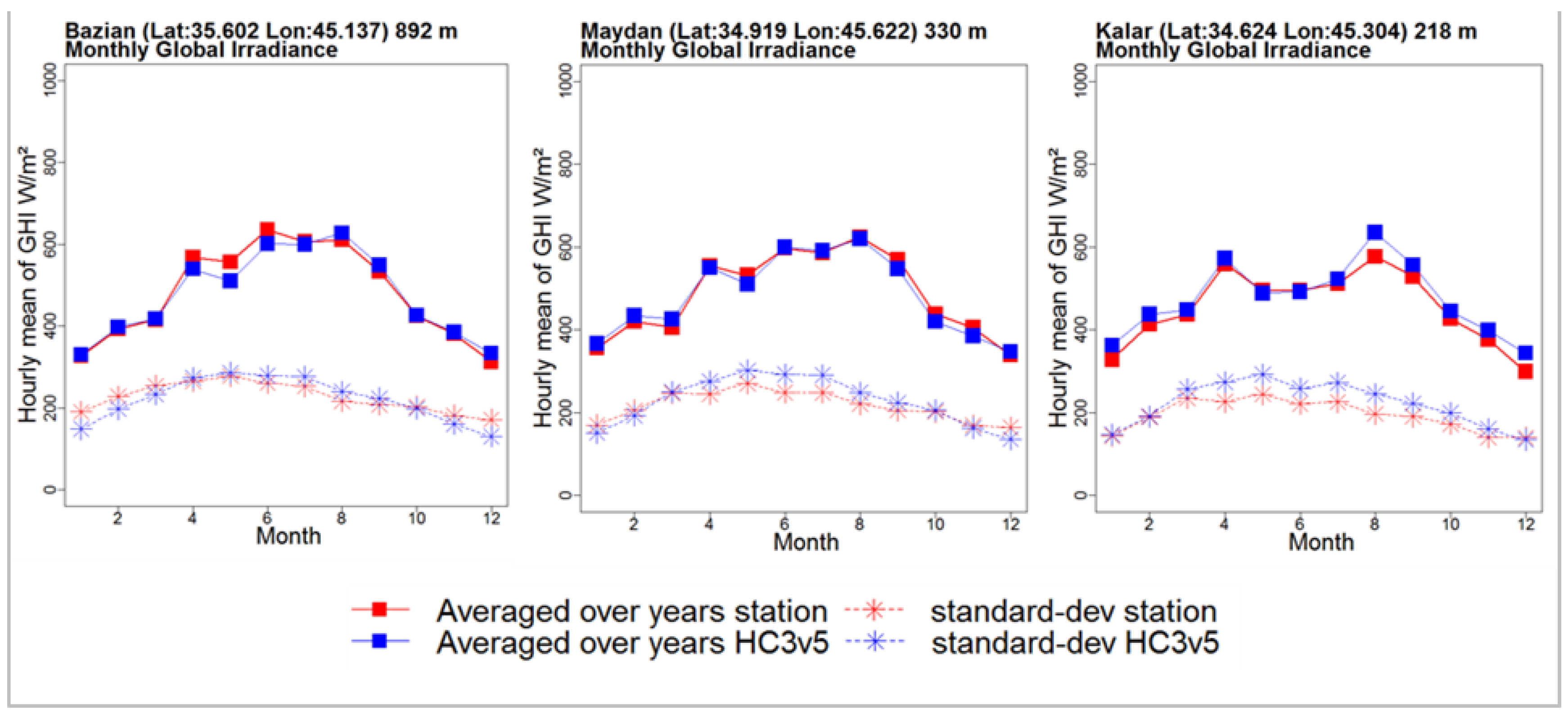
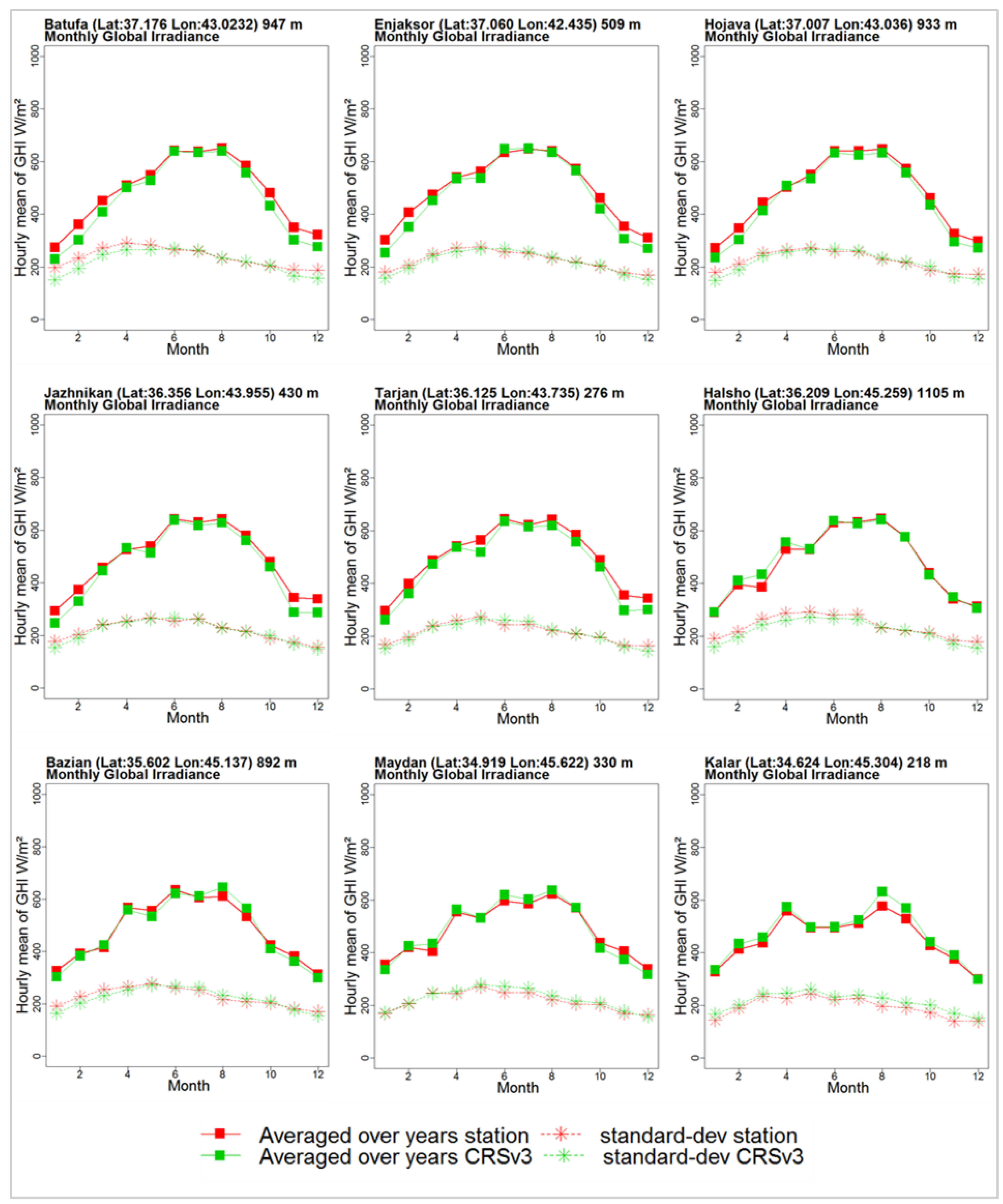
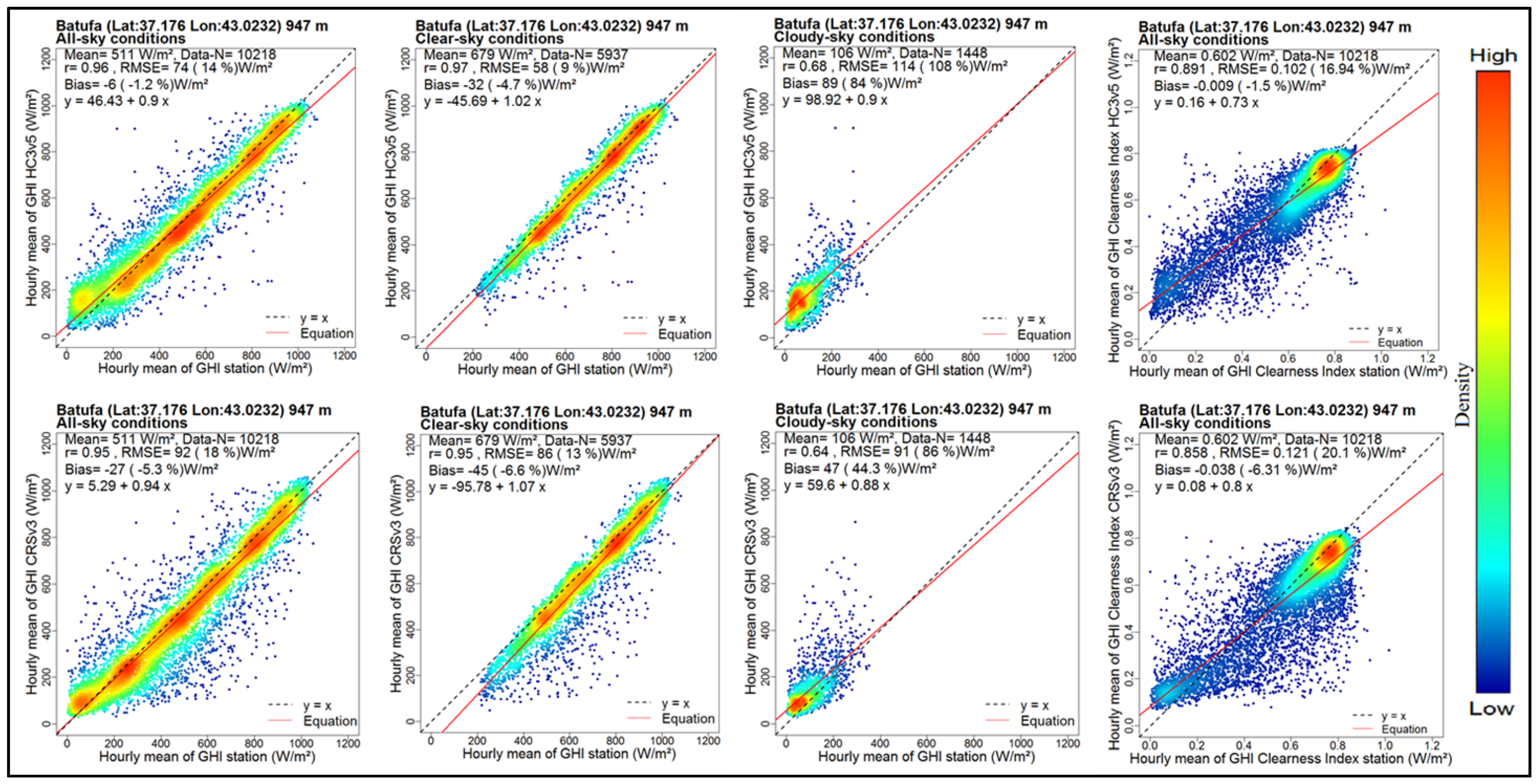
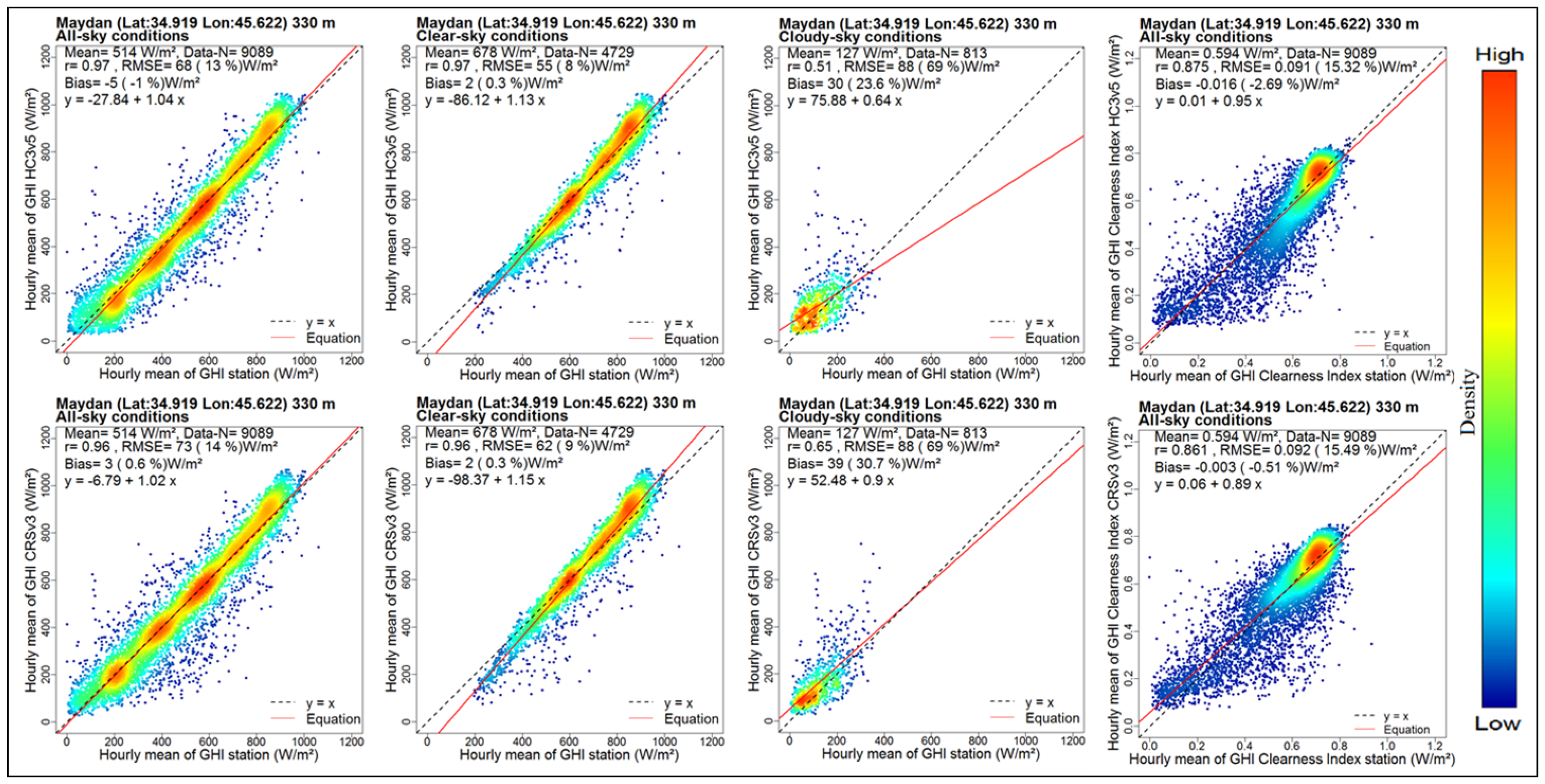
3.1. All-Sky Conditions

The results of the validation for the all-sky conditions are presented in Table 3. The correlation is from 0.94 to 0.97 in all of the stations and 0.92–0.97 in the points around them. Interestingly, zero bias was recorded at Hojava station, and it was near zero in several other cases (Halsho, Maydan and Bazian stations) for both SDDs. Negative (underestimation) bias was recorded in several cases. It ranges from −21 W/m² (−4%) to −3 W/m² (−0.6%) for HC3v5, which is lower than CRSv3 in most cases, which ranges from −27 W/m² (−5.3%) to −2 W/m² (−0.4%). Moreover, it was lower than −6% for all of the stations. However, a positive (overestimation) bias was recorded in some of the cases. The highest case of bias in the study was recorded at Kalar station, which was 25 W/m² (5.3%) for CRSv3 and 21 W/m² (4.4%) for HC3v5. Some other positive rates were recorded at Halsho and Maydan stations, which were lower than 2% for both SDDs (Figure 7, Table 3).

The bias at each station was compared to the points around the station, and was nearly the same with no more than 4% difference for each station. Overall, the rate of bias in HC3v5 was less than that in CRSv3 (Figure 7, Table 3).

The RMSE was under 21% in all of the cases. Its lowest range, at Enjaksor, was 64 W/m² (12%), and increased to the highest value of 88 W/m² (19%) at Kalar station for HC3v5. It was generally high for CRSv3 ranging from 71 W/m² (14%) to 100 W/m² (20%). Most of the other rates of RMSE were between 14−18% for both SDDs.

The RMSE for the points around the stations compared to the station location are nearly the same (Figure 8). Overall, the RMSE for HC3v5 was less than that for CRSv3 (Figure 8).

The smooth scatter density plot illustrates the residual and correlation between ground data and SDDs in some cases. For example, Figure 9 for Batufa station shows that the density of observations were mostly under the 1:1 line, which indicated a recorded negative bias, and the RMSE was acceptable for HC3v5 and high for CRSv3, while some of the other values above the 1:1 line are under 200 W/m². However, Figure 10 (Kalar station) shows that the majority of observations are above the 1:1 line and some points are far from the line. This corresponds to positive bias and high RMSE in the station.

Low rates of bias and RMSE were recorded at Maydan station, which is shown in Figure 11 for HC3v5 and CRSv3 respectively. The best-fit line in red is nearly the same as the 1:1 line, more so for HC3v5 than CRSv3 (at the same station).

The results of the clearness index in the all-sky conditions are represented in Table 4. The percentages of bias and RMSE were quite similar to the GHI. Hence, the r values at all of the stations were lower than the GHI, which ranged from 0.82–0.89. The r values were higher in HC3v3 than CRSv3 when comparing each station for both. The scatter density plot shows the highest density of observations at around 0.7 W/m² for all of the stations. Negative bias at Batufa, Maydan and positive bias at Kalar can be seen, although the values were low. Several values are far from the 1:1 line, resulting in RMSE to be from 15–21% at all of the stations (Figure 9, Figure 10 and Figure 11).

Results of the mean and standard deviation of the GHI in months are represented in Figure 5 for HC3v5 and in Figure 6 for CRSv3. The two figures demonstrate the distribution of the two SDDs with ground data in each month, expressed by the standard deviation. However, some differences were recorded in the winter months at Batufa, Hojava, Halsho and Bazian stations, whereas for summer months differences were recorded at Maydan and Kalar stations for both SDDs.

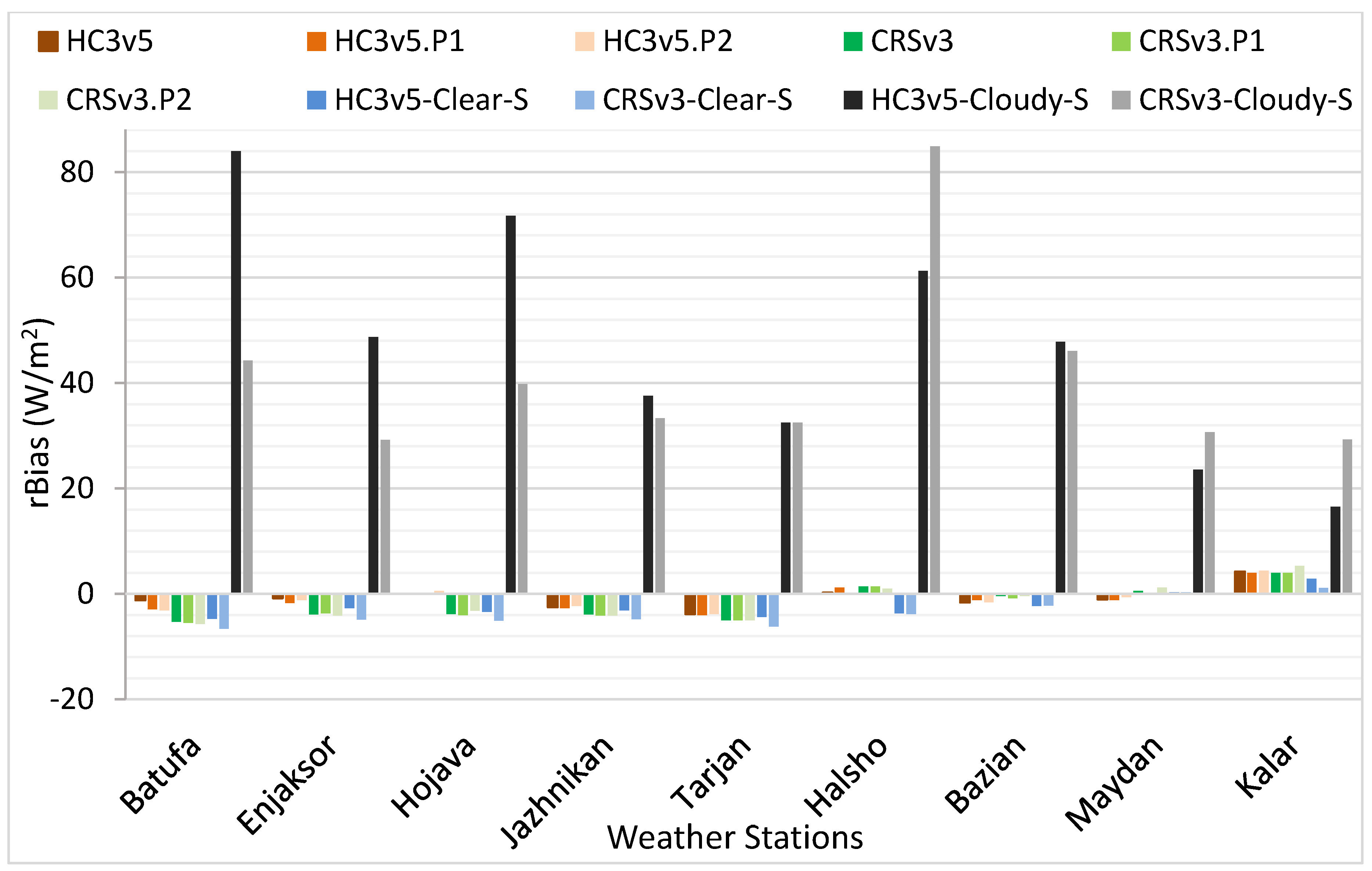
3.2. Clear-Sky and Cloudy-Sky Conditions

The compared results of the two SDDs for clear-sky and cloudy-sky conditions are presented in Table 5. There are apparent differences in the r values between the clear-sky and cloudy-sky conditions in all of all cases. These ranged from 0.95–0.97 for clear-skies, whereas for the cloudy-skies, it ranged from 0.51–0.72 among the stations.

Similarly, the ranges of bias were much higher in the cloudy-skies than in the clear-skies. The lowest bias was a 2 W/m² (0.3%) overestimation at Maydan in clear-sky conditions whereas in the same station it reached 30 W/m² (24%) in cloudy-sky conditions. The highest bias for the clear-sky conditions was recorded at Batufa station, which was −32 W/m² (−4.7%). The same station had the highest bias for the cloudy-sky conditions, which was 89 W/m² (84%). These were recorded for HC3v5. The bias for CRSv3 was the same as HC3v3 for the low range in the clear-sky conditions. In others, the ranges start from −45 W/m² (−6.6%) underestimation at Batufa station to 7 W/m² (1%) overestimation at Kalar station, while for cloudy-skies, it ranged from 33 (29%) to 90 (85%) W/m² respectively. The variety of the two SDDs in term of bias is shown in Figure 7, which illustrates a moderate difference between cloudy-sky and clear-sky conditions from one station to the other. In addition, the range of bias was much lower in clear-skies than cloudy-skies and the bias in all-sky conditions was lower than that in clear-skies except for two stations for both SDDs where the bias was higher to some degree in the all-sky conditions than in the clear-skies (Figure 7).

Similarly, the RMSE was much higher in the cloudy-skies than in clear-skies for the SDDs in each station. For example, at Halsho station for CRSv3 it was 61 W/m² (9%) in clear-skies and increased sharply to 127 W/m² (120%) under cloudy conditions. Nearly the same situation can be seen for Batufa station for HC3v5. The RMSE for both SDDs was lower than 14% at all of the stations for the clear-skies while it was above 58% for the cloudy-skies (Figure 8, Table 5). The RMSE in clear-skies was lower than in the case of all-sky conditions in all of the study areas for both SDDs (Figure 8).

The smooth scatter density plot for Batufa, Kalar and Maydan of both SDDs separately shows that the density of observations were above the 1:1 line, and the direction of distribution was towards the high value of SDD which recorded high overestimation and high RMSE in cloudy-sky conditions (Figure 9, Figure 10 and Figure 11). In contrast, in the clear-sky conditions for nearly all of the stations, the distribution of observations was near the 1:1 line. This leads to low RMSE in clear-skies compared to cloudy-sky and all-sky conditions (Figure 9, Figure 10 and Figure 11). The observations under the 1:1 line illustrated a negative bias at Batufa station, whereas the opposite—i.e., positive bias—occurred at Kalar station, and a minimal bias was seen at Maydan station relative to the normal distribution.

Overall, the results of the validation varied from one station to another, and they are acceptable according to bias and RMSE. At some stations, the results were disappointing. The points around the stations had nearly the same ranges of bias and RMSE compared to the station location. In most of the cases, the bias and RMSE of HC3v5 were lower than CRSv3. The bias and RMSE were lower for the clear-sky and all-sky conditions than for the cloudy-skies.

4. Discussion

The validation results demonstrate good agreement between the ground data and SDDs in all-sky and clear-sky conditions (average r = 0.95, bias under 6% and RMSE under 21%), unlike the results for the cloudy-sky conditions (average r = 0.61, bias above 16% and RMSE above 61%). The results from the two neighbouring points at each station are close to the results at the station location with an average difference of 2%. Overall the performance of SDDs are in agreement with those from similar studies in other areas [39,41,42,48], also showing a better performance for HC3v5 over CRSv3 (Figure 7 and Figure 8). This is mainly related to the inputs into the models for creating each dataset, whether it is H2 or H4 (see Section 2.3).

4.1. All-Sky Conditions

The high rates of positive bias and RMSE at Kalar compared to all of the other stations (Figure 7, Figure 8, Figure 9, Figure 10 and Figure 11) might be due to the quality of the recorded data [46] and a partial shadow on the sensor at that station, because its mean is lower than that at the other stations by nearly 30 W/m² (Table 3), while those data have passed the quality check. However, a similar positive bias and RMSE are reported by other studies [41,42]. The low rates of bias (0–2%) were recorded for HC3v5 at the stations of Hojava, Halsho, Bazian and Maydan, and for CRSv3 for the same stations except for Hojava, whose bias rate reaches −3.8% for all-sky conditions (Table 3, Figure 7). These show that the GHI ground data are explained well by satellite data (Figures S1–S5), while the resolution of satellite imagery in that area is 5 km (Figure 2). The underestimations of bias (1–6%) and RMSE (12–20%) were recorded at most stations (Table 3, Figure 7 and Figure 8). Comparable percentages were recorded in similar studies in other areas and climate regions, namely Egypt [41], Brazil [39], and some BSRN stations [48]. The reasons are partly related to the local condition of the station, inputs to the Heliosat method—especially the atmospheric optical depth owing to its unavailability—, various cloud types, the resolution of satellite images and the aerosols effect [37,39,55]. This is because in some cases, the GHI ground data are well explained by SDDs (Figures S1–S5), but in other cases only some error rates were recorded (Table 3). Those rates are quite reasonable for hourly GHI [42]. Those rates of bias can be corrected or modified in some ways [14,18,56,57].

The low variabilities between the ground data and both SDDs are seen in Figure 5 and Figure 6. This might be related to the geographical location and climatic condition, and another reason is that the data were aggregated, concealing some random errors between the two datasets. Hence, some error rates in winter months are related to the difficulty of the Heliosat methods to estimate GHI in cloudy conditions [31,51]. The performance of the clearness index (Table 4) is nearly the same for GHI in at all-sky conditions, which is related to the above-mentioned reasons.

The interesting side of this study is that the results of the validation for both SDDs with the two neighbouring points at each station separately are slightly closer to those at the station location. The differences range between 0–2% for bias and RMSE for each point at most of the locations (Table 3, Figure 7 and Figure 8). The ±1–4% difference between the station location and the neighbouring points with the station ground data GHI are mainly related to the elevation above sea level for each location. Other factors might be related to local land surface types such as land and water, agriculture and bare soil. This indicates that the GHI from SDDs can be used for regional planning for various purposes, and the ground data GHI can be used for neighbouring areas when there is a limitation of ground data. This validation is also considered to add further weight to the assumption of near uniformity of solar radiation in a 25 km² area [23,53].

4.2. Clear-Sky and Cloudy-Sky Conditions

The validation results for both SDDs of GHI with the ground data for clear-sky conditions showed good agreement according to RMSE, which decreased at most stations (Figure 7, Figure 8, Figure 9, Figure 10 and Figure 11). This is partly related to the inputs to the H2 method, especially in incorporating the visible images of MSG in cloud-free conditions into the model. Similarly, the increased performance of HC3v5 for clear-sky conditions has been reported [41] in Egypt. However, the remaining residuals of clear-sky conditions are caused by the factors that have been mentioned in the all-sky conditions above. However, the bias increased to some degree for both SDDs in most of the stations, which were recording underestimations for clear-sky conditions. This is partially related to the increase of the mean GHI ground data in clear-sky conditions. It has also been recorded by several studies [19,27,37], which show that the bias is underestimated for clear-skies.

The study investigated the performance of SDDs on cloudy-sky conditions, reflected in the very low performance of both HC3v5 and CRSv3 according to the high ratio of bias and RMSE (Figure 7 and Figure 8). A close look at the samples of smooth scatter plots (Figure 9, Figure 10 and Figure 11) shows how far the observations and their density are from the 1:1 line. This is related to difficulties in analysing cloudy pixels of MSG images [31]; the clouds prevented the ground being viewed from the sensor aboard the satellite [42], and as such it is hard to differentiate between cloud albedo and ground albedo [51]. These factors lead to an overestimation of GHI as shown in all of the stations (Table 5) for bias, and much higher RMSE (Figure 6 and Figure 7). Indeed, in some of the cases, it is above the mean of the observations. Similar high residuals for cloudy conditions have been reported in the literature [19,27,37,41]. This indicates that the GHI ground data are well explained by the SDDs in clear-sky conditions, whereas they are not explained well in cloudy-sky conditions (Figures S6–S15). The results of high bias and RMSE indicate that further research is required to correct the errors under cloudy-sky conditions, whereas several studies have done bias corrections for all-sky conditions [14,18,56,57].

The limitations of this study are the different data timescales from one station to another and the limited information available for some parameters, such as the aerosols and local atmospheric properties. This might lead to a challenge to fully explain the reasons behind the results at each station.

However, the validation results vary from one station to another and are near the World Meteorological Organisation (WMO) standard, whereby the bias should be less than 3 W/m² and 95% of errors should not exceed 20 W/m² [50]. However, the validation results in a minority of stations are above the WMO standard. Therefore, it is probable that the SDDs can be used for modelling and mapping solar radiation with some modification and bias correction.

5. Conclusions

The study has validated hourly GHI from two SDDs, which are HC3v5 and CRSv3, with ground data from nine stations in northeast Iraq for all-sky, clear-sky and cloudy-sky conditions in the station pixels and with two other pixels around the station in all-sky conditions. The temporal changes of ground data GHI were well represented by both SDDs; r was above 0.94 for the all-sky and clear-sky conditions, and above 0.82 for the clearness index in most cases, while for cloudy-skies it was between 0.51–0.72. The bias was negative (underestimation) for most of the cases except for two HC3v5 and three CRSv3 cases, in which it was positive (overestimation); all of the bias ranges were smaller than 8% (W/m²) of the mean GHI in all-sky and clear-sky conditions, whereas for cloudy-sky conditions, it was positive and varied from one station to another, by 17–85% (W/m²) of the mean GHI. The same applies to RMSE. It ranged between 8–20% (W/m²) in all of the stations for all-sky and clear-sky conditions. In contrast, the range was much higher in cloudy-sky conditions: above 56%. The differences between neighbouring pixels and at-station pixels in the SDDs compared to the ground data of GHI for each site are very small, varying by 2% in most cases. The overall performance of HC3v5 is better than that of CRSv3.

Despite the ratio of errors at some stations, the SDDs are closely related to the ground data at most of the stations. However, the resolution of MSG images is 5 km in the case study. The SDDs represent hourly GHI well, and this can be used to map solar resources and possibly for modelling GHI with ground data in areas with a low number of stations.

Further studies about the bias corrections in the SDDs are needed, especially for cloudy-sky conditions. Further research would also be useful for validating the SDDs in other climates. Some studies are also required to address the inputs to the Heliosat method, according to regional and local factors, for a better estimation of GHI from satellite images.

References

1. Despotovic, M.; Nedic, V.; Despotovic, D.; Cvetanovic, S. Evaluation of empirical models for predicting monthly mean horizontal diffuse solar radiation. Renew. Sustain. Energy Rev. 2016, 56, 246–260. [Google Scholar] [CrossRef]
2. Kanters, J.; Wall, M. A planning process map for solar buildings in urban environments. Renew. Sustain. Energy Rev. 2016, 57, 173–185. [Google Scholar] [CrossRef]
3. Mohanty, S.; Patra, P.K.; Sahoo, S.S. Prediction and application of solar radiation with soft computing over traditional and conventional approach—A comprehensive review. Renew. Sustain. Energy Rev. 2016, 56, 778–796. [Google Scholar] [CrossRef]
4. Paulescu, E.; Blaga, R. Regression models for hourly diffuse solar radiation. Sol. Energy 2016, 125, 111–124. [Google Scholar] [CrossRef]
5. Polo, J.; Zarzalejo, L.; Cony, M.; Navarro, A.; Marchante, R.; Martin, L.; Romero, M. Solar radiation estimations over India using meteosat satellite images. Sol. Energy 2011, 85, 2395–2406. [Google Scholar] [CrossRef]
6. Urraca, R.; Martinez-de-Pison, E.; Sanz-Garcia, A.; Antonanzas, J.; Antonanzas-Torres, F. Estimation methods for global solar radiation: Case study evaluation of five different approaches in central Spain. Renew. Sustain. Energy Rev. 2017, 77, 1098–1113. [Google Scholar] [CrossRef]
7. Gherboudj, I.; Ghedira, H. Assessment of solar energy potential over the united arab emirates using remote sensing and weather forecast data. Renew. Sustain. Energy Rev. 2016, 55, 1210–12224. [Google Scholar] [CrossRef]
8. Qin, J.; Chen, Z.; Yang, K.; Liang, S.; Tang, W. Estimation of monthly-mean daily global solar radiation based on modis and trmm products. Appl. Energy 2011, 88, 2480–2489. [Google Scholar] [CrossRef]
9. Xie, Y.; Yu, T.; Gu, X.; Zhao, L.; Zhang, L.; Wang, G. The estimation of surface daily reflected solar radiation using landsat-7 etm+ and empirical models. In Proceedings of the 2012 5th International Congress on Image and Signal Processing (CISP), Chongqing, China, 16–18 October 2012; IEEE: Piscataway, NJ, USA, 2012; pp. 1109–1113. [Google Scholar]
10. Cano, D.; Monget, J.-M.; Albuisson, M.; Guillard, H.; Regas, N.; Wald, L. A method for the determination of the global solar radiation from meteorological satellite data. Sol. Energy 1986, 37, 31–39. [Google Scholar] [CrossRef] [Green Version]
11. Rigollier, C.; Lefèvre, M.; Wald, L. The method heliosat-2 for deriving shortwave solar radiation from satellite images. Sol. Energy 2004, 77, 159–169. [Google Scholar] [CrossRef]
12. Beyer, H.G.; Costanzo, C.; Heinemann, D. Modifications of the heliosat procedure for irradiance estimates from satellite images. Sol. Energy 1996, 56, 207–212. [Google Scholar] [CrossRef]
13. Eissa, Y.; Chiesa, M.; Ghedira, H. Assessment and recalibration of the heliosat-2 method in global horizontal irradiance modeling over the desert environment of the UAE. Sol. Energy 2012, 86, 1816–1825. [Google Scholar] [CrossRef]
14. Qu, Z.; Gschwind, B.; Lefevre, M.; Wald, L. Improving helioclim-3 estimates of surface solar irradiance using the mcclear clear-sky model and recent advances in atmosphere composition. Atmos. Meas. Tech. 2014, 7, 3927–3933. [Google Scholar] [CrossRef] [Green Version]
15. Janjai, S.; Pankaew, P.; Laksanaboonsong, J. A model for calculating hourly global solar radiation from satellite data in the tropics. Appl. Energy 2009, 86, 1450–1457. [Google Scholar] [CrossRef]
16. Janjai, S. A method for estimating direct normal solar irradiation from satellite data for a tropical environment. Sol. Energy 2010, 84, 1685–1695. [Google Scholar] [CrossRef]
17. Janjai, S.; Pankaew, P.; Laksanaboonsong, J.; Kitichantaropas, P. Estimation of solar radiation over cambodia from long-term satellite data. Renew. Energy 2011, 36, 1214–1220. [Google Scholar] [CrossRef]
18. Polo, J.; Wilbert, S.; Ruiz-Arias, J.A.; Meyer, R.; Gueymard, C.; Suri, M.; Martín, L.; Mieslinger, T.; Blanc, P.; Grant, I. Preliminary survey on site-adaptation techniques for satellite-derived and reanalysis solar radiation datasets. Sol. Energy 2016, 132, 25–37. [Google Scholar] [CrossRef]
19. Zhang, X.; Liang, S.; Wang, G.; Yao, Y.; Jiang, B.; Cheng, J. Evaluation of the reanalysis surface incident shortwave radiation products from NCEP, ECMWF, GSFC, and JMA using satellite and surface observations. Remote Sens. 2016, 8, 225. [Google Scholar] [CrossRef]
20. Polo, J. Solar global horizontal and direct normal irradiation maps in Spain derived from geostationary satellites. J. Atmos. Sol.-Terr. Phys. 2015, 130–131, 81–88. [Google Scholar] [CrossRef]
21. Journée, M.; Bertrand, C. Geostatistical merging of ground-based and satellite-derived data of surface solar radiation. Adv. Sci. Res. 2011, 6, 1–5. [Google Scholar] [CrossRef] [Green Version]
22. Journée, M.; Müller, R.; Bertrand, C. Solar resource assessment in the Benelux by merging meteosat-derived climate data and ground measurements. Sol. Energy 2012, 86, 3561–3574. [Google Scholar] [CrossRef]
23. Bojanowski, J.S.; Vrieling, A.; Skidmore, A.K. Calibration of solar radiation models for Europe using meteosat second generation and weather station data. Agric. For. Meteorol. 2013, 176, 1–9. [Google Scholar] [CrossRef]
24. Roerink, G.J.; Bojanowski, J.S.; de Wit, A.J.W.; Eerens, H.; Supit, I.; Leo, O.; Boogaard, H.L. Evaluation of Msg-derived global radiation estimates for application in a regional crop model. Agric. For. Meteorol. 2012, 160, 36–47. [Google Scholar] [CrossRef]
25. Sanchez-Lorenzo, A.; Wild, M.; Brunetti, M.; Guijarro, J.A.; Hakuba, M.Z.; Calbó, J.; Mystakidis, S.; Bartok, B. Reassessment and update of long-term trends in downward surface shortwave radiation over Europe (1939–2012). J. Geophys. Res. Atmos. 2015, 120, 9555–9569. [Google Scholar] [CrossRef]
26. Sanchez-Lorenzo, A.; Wild, M.; Trentmann, J. Validation and stability assessment of the monthly mean cm SAF surface solar radiation dataset over Europe against a homogenized surface dataset (1983–2005). Remote Sens. Environ. 2013, 134, 355–366. [Google Scholar] [CrossRef]
27. Amillo, A.; Huld, T.; Müller, R. A new database of global and direct solar radiation using the Eastern Meteosat Satellite, models and validation. Remote Sens. 2014, 6, 8165–8189. [Google Scholar] [CrossRef] [Green Version]
28. Riihelä, A.; Carlund, T.; Trentmann, J.; Müller, R.; Lindfors, A. Validation of cm SAF surface solar radiation datasets over Finland and Sweden. Remote Sens. 2015, 7, 6663–6682. [Google Scholar] [CrossRef]
29. Ineichen, P.; Barroso, C.S.; Geiger, B.; Hollmann, R.; Marsouin, A.; Mueller, R. Satellite application facilities irradiance products: Hourly time step comparison and validation over Europe. Int. J. Remote Sens. 2009, 30, 5549–5571. [Google Scholar] [CrossRef]
30. Moradi, I.; Mueller, R.; Alijani, B.; Kamali, G.A. Evaluation of the heliosat-II method using daily irradiation data for four stations in Iran. Sol. Energy 2009, 83, 150–156. [Google Scholar] [CrossRef]
31. Schillings, C.; Meyer, R.; Mannstein, H. Validation of a method for deriving high resolution direct normal irradiance from satellite data and application for the arabian peninsula. Sol. Energy 2004, 76, 485–497. [Google Scholar] [CrossRef]
32. AL-Jumaily, K.J.; AL-Salihi, A.M.; Al-Tai, O.T. Evaluation of meteosat-8 measurements using daily global solar radiation for two stations in iraq. Energy Environ. 2010, 1, 635–642. [Google Scholar]
33. Riihelä, A.; Kallio, V.; Devraj, S.; Sharma, A.; Lindfors, A. Validation of the Sarah-e satellite-based surface solar radiation estimates over India. Remote Sens. 2018, 10, 392. [Google Scholar] [CrossRef]
34. Gueymard, C.A.; Wilcox, S.M. Assessment of spatial and temporal variability in the US solar resource from radiometric measurements and predictions from models using ground-based or satellite data. Sol. Energy 2011, 85, 1068–1084. [Google Scholar] [CrossRef]
35. Habte, A.; Sengupta, M.; Wilcox, S. Comparing measured and satellite-derived surface irradiance. In Proceedings of the ASME 2012 6th International Conference on Energy Sustainability collocated with the ASME 2012 10th International Conference on Fuel Cell Science, Engineering and Technology, San Diego, CA, USA, 23–26 July 2012; American Society of Mechanical Engineers: New York, NY, USA, 2012; pp. 561–566. [Google Scholar]
36. Lave, M.; Weekley, A. Comparison of high-frequency solar irradiance: Ground measured vs. In Satellite-derived. In Proceedings of the 2016 IEEE 43rd Photovoltaic Specialists Conference (PVSC), Portland, OR, USA, 5–10 June 2016; IEEE: Piscataway, NJ, USA, 2016; pp. 1101–1106. [Google Scholar]
37. Xia, S.; Mestas-Nuñez, A.; Xie, H.; Vega, R. An evaluation of satellite estimates of solar surface irradiance using ground observations in San Antonio, Texas, USA. Remote Sens. 2017, 9, 1268. [Google Scholar] [CrossRef]
38. SoDa. Solar Radiation Data. Available online: http://www.soda-pro.com/ (accessed on 20 March 2017).
39. Thomas, C.; Wey, E.; Blanc, P.; Wald, L. Validation of three satellite-derived databases of surface solar radiation using measurements performed at 42 stations in Brazil. Adv. Sci. Res. 2016, 13, 81–86. [Google Scholar] [CrossRef] [Green Version]
40. Thomas, C.; Saboret, L.; Wey, E.; Blanc, P.; Wald, L. Validation of the new helioclim-3 version 4 real-time and short-term forecast service using 14 BSRN stations. Adv. Sci. Res. 2016, 13, 129–136. [Google Scholar] [CrossRef] [Green Version]
41. Eissa, Y.; Korany, M.; Aoun, Y.; Boraiy, M.; Abdel Wahab, M.; Alfaro, S.; Blanc, P.; El-Metwally, M.; Ghedira, H.; Hungershoefer, K.; et al. Validation of the surface downwelling solar irradiance estimates of the helioclim-3 database in egypt. Remote Sens. 2015, 7, 9269–9291. [Google Scholar] [CrossRef] [Green Version]
42. Marchand, M.; Al-Azri, N.; Ombe-Ndeffotsing, A.; Wey, E.; Wald, L. Evaluating meso-scale change in performance of several databases of hourly surface irradiation in south-eastern Arabic Pensinsula. Adv. Sci. Res. 2017, 14, 7–15. [Google Scholar] [CrossRef]
43. Kottek, M.; Grieser, J.; Beck, C.; Rudolf, B.; Rubel, F. World map of the köppen-geiger climate classification updated. Meteorol. Z. 2006, 15, 259–263. [Google Scholar] [CrossRef]
44. GDMS. Ministry of Transport and Communications 2016. General Directorate of Meteorology & Seismology. Available online: http://gdms-krg.org/ku/ (accessed on 14 May 2017).
45. Long, C.N.; Dutton, E.G. BSRN Global Network Recommended QC Tests; v2.0; PANGAEA: Bremerhaven, Germany, 2002. [Google Scholar]
46. Ameen, B.; Balzter, H.; Jarvis, C. Quality control of global horizontal irradiance estimates through bsrn, toacs and air temperature/sunshine duration test procedures. Climate 2018, 6, 69. [Google Scholar] [CrossRef]
47. Geiger, M.; Diabaté, L.; Ménard, L.; Wald, L. A web service for controlling the quality of measurements of global solar irradiation. Sol. Energy 2002, 73, 475–480. [Google Scholar] [CrossRef] [Green Version]
48. Thomas, C.; Wey, E.; Blanc, P.; Wald, L.; Lefèvre, M. Validation of helioclim-3 version 4, helioclim-3 version 5 and macc-rad using 14 bsrn stations. Energy Procedia 2016, 91, 1059–1069. [Google Scholar] [CrossRef] [Green Version]
49. Eissa, Y.; Munawwar, S.; Oumbe, A.; Blanc, P.; Ghedira, H.; Wald, L.; Bru, H.; Goffe, D. Validating surface downwelling solar irradiances estimated by the mcclear model under cloud-free skies in the United Arab Emirates. Sol. Energy 2015, 114, 17–31. [Google Scholar] [CrossRef] [Green Version]
50. Lefèvre, M.; Wald, L. Validation of the mcclear clear-sky model in desert conditions with three stations in Israel. Adv. Sci. Res. 2016, 13, 21–26. [Google Scholar] [CrossRef] [Green Version]
51. Blanc, P.; Gschwind, B.; Lefèvre, M.; Wald, L. The helioclim project: Surface solar irradiance data for climate applications. Remote Sens. 2011, 3, 343–361. [Google Scholar] [CrossRef] [Green Version]
52. Mueller, R.; Trentmann, J.; Träger-Chatterjee, C.; Posselt, R.; Stöckli, R. The role of the effective cloud albedo for climate monitoring and analysis. Remote Sens. 2011, 3, 2305–2320. [Google Scholar] [CrossRef]
53. Bouchouicha, K.; Razagui, A.; Bachari, N.E.I.; Aoun, N. Estimation of hourly global solar radiation using msg-hrv images. Int. J. Appl. Environ. Sci. 2016, 11, 351–368. [Google Scholar]
54. Quej, V.H.; Almorox, J.; Arnaldo, J.A.; Saito, L. Anfis, svm and ann soft-computing techniques to estimate daily global solar radiation in a warm sub-humid environment. J. Atmos. Sol.-Terr. Phys. 2017, 155, 62–70. [Google Scholar] [CrossRef]
55. Kaskaoutis, D.G.; Kambezidis, H.D.; Dumka, U.C.; Psiloglou, B.E. Dependence of the spectral diffuse-direct irradiance ratio on aerosol spectral distribution and single scattering albedo. Atmos. Res. 2016, 178–179, 84–94. [Google Scholar] [CrossRef]
56. Frank, C.W.; Wahl, S.; Keller, J.D.; Pospichal, B.; Hense, A.; Crewell, S. Bias correction of a novel european reanalysis data set for solar energy applications. Sol. Energy 2018, 164, 12–24. [Google Scholar] [CrossRef]
57. Polo, J.; Martín, L.; Vindel, J.M. Correcting satellite derived dni with systematic and seasonal deviations: Application to India. Renew. Energy 2015, 80, 238–243. [Google Scholar] [CrossRef]
Figure 1. Climate regions, station types, and their distribution in the study area [43,44].
Remotesensing 10 01651 g001
Figure 2. Spatial coverage of the SEVIRI instrument for MSG images [38].
Remotesensing 10 01651 g002
Figure 3. The flowchart of the approach.
Remotesensing 10 01651 g003
Figure 4. Example of point pixel selection of SDD around Bazian station.
Remotesensing 10 01651 g004
Figure 5. Monthly mean and standard deviation of hourly GHI data in each month aggregated over the data availability for each station with HC3v5. The difference between dots reveals the errors in a month and vice versa. If the dot of the SDD in a month is above the dot of the ground data, it denotes overestimation; otherwise, it denotes underestimation.
Remotesensing 10 01651 g005aRemotesensing 10 01651 g005b
Figure 6. Monthly mean and standard deviation of hourly GHI data in each month aggregated over data availability for each station with CRSv5. The difference between dots reveals errors in a month and vice versa. If the dot of the SDD in a month is above the dot of the ground data, it denotes overestimation; otherwise, it denotes underestimation.
Remotesensing 10 01651 g006
Figure 7. Comparison of rBias for the hourly GHI for all-sky conditions among stations with points around them for HC3v5 and CRSv3. Clear-skies and cloudy-skies at stations are represented by blue, light blue, black and grey colours, respectively.
Remotesensing 10 01651 g007
Figure 8. As in Figure 7, but for rRMSE.
Remotesensing 10 01651 g008
Figure 9. Scatter plot between hourly GHI ground measurements and SDDs (HC3v5 and CRSv3) for Batufa station for all-sky, clear-sky and cloudy-sky conditions and the clearness index.
Remotesensing 10 01651 g009
Figure 10. Scatter plot between hourly GHI ground measurements and SDDs (HC3v5 and CRSv3) for Kalar station for all-sky, clear-sky and cloudy-sky conditions and the clearness index.
Remotesensing 10 01651 g010
Figure 11. Scatter plot between hourly GHI ground measurements and SDDs (HC3v5 and CRSv3) for Maydan station for all-sky, clear-sky and cloudy-sky conditions and the clearness index.
Remotesensing 10 01651 g011