Upscaling Solar-Induced Chlorophyll Fluorescence from an Instantaneous to Daily Scale Gives an Improved Estimation of the Gross Primary Productivity

Abstract

Solar-induced chlorophyll fluorescence (SIF) is closely linked to the photosynthesis of plants and has the potential to estimate gross primary production (GPP) at different temporal and spatial scales. However, remotely sensed SIF at a ground or space level is usually instantaneous, which cannot represent the daily total SIF. The temporal mismatch between instantaneous SIF (SIF_inst) and daily GPP (GPP_daily) impacts their correlation across space and time. Previous studies have upscaled SIF_inst to the daily scale based on the diurnal cycle in the cosine of the solar zenith angle ($\cos \left(\mathrm{SZA}\right)$) to correct the effects of latitude and length of the day on the variations in the SIF-GPP correlation. However, the important effects of diurnal weather changes due to cloud and atmospheric scattering were not considered. In this study, we present a SIF upscaling method using photosynthetically active radiation (PAR) as a driving variable. First, a conversion factor (i.e., the ratio of the instantaneous PAR (PAR_inst) to daily PAR (PAR_daily)) was used to upscale in-situ SIF measurements from the instantaneous to daily scale. Then, the performance of the SIF upscaling method was evaluated under changing weather conditions and different latitudes using continuous tower-based measurements at two sites. The results prove that our PAR-based method can reduce not only latitude-dependent but also the weather-dependent variations in the SIF-GPP model. Specifically, the PAR-based method gave a more accurate prediction of diurnal and daily SIF (SIF_daily) than the $\cos \left(\mathrm{SZA}\right)$-based method, with decreased relative root mean square error (RRMSE) values from 42.2% to 25.6% at half-hour intervals and from 25.4% to 13.3% at daily intervals. Moreover, the PAR-based upscaled SIF_daily had a stronger correlation with the daily absorbed PAR (APAR) than both the SIF_inst and $\cos \left(\mathrm{SZA}\right)$-based upscaled SIF_daily, especially for cloudy days with a coefficient of determination (R²) that increased from approximately 0.5 to 0.8. Finally, the PAR-based SIF_daily was linked to GPP_daily and compared to the SIF_inst or $\cos \left(\mathrm{SZA}\right)$-based SIF_daily. The results indicate that the SIF-GPP correlation can obviously be improved, with an increased R² from approximately 0.65 to 0.75. Our study confirms the importance of upscaling SIF from the instantaneous to daily scale when linking SIF with GPP and emphasizes the need to take diurnal weather changes into account for SIF temporal upscaling.

1. Introduction

Photosynthesis, which supports most life on earth [1], is a vital process driving the global carbon cycle [2]. The explicit estimation of the photosynthetic exchange flux, known as gross primary productivity (GPP), can offer key information for exploring and quantifying terrestrial carbon fixation by plants [3]. The eddy covariance (EC) technique makes it possible to measure the carbon dioxide (CO₂) exchange between vegetation and the atmosphere and partition it into GPP and ecosystem respiration [4]. However, EC flux towers are dispersed and only cover very limited regions. Remote sensing offers the unique possibility of deriving the continuous global monitoring of carbon exchange. Currently, global GPP can be estimated using a light use efficiency (LUE) model, which combines reflectance-based remote sensing and climate variables [5,6]; a data-driven method, which integrates EC flux observations, remote sensing and climate data [2,7]; process-based models [8,9]. However, uncertainties in the diagnostic models, measured variables, and auxiliary products all propagate into the global GPP estimation, which limits the monitoring power of these methods [2,10].

The remote measurements of sun-induced chlorophyll fluorescence (SIF) offer a new tool for monitoring vegetation photosynthesis. SIF refers to the emission of red and far-red light from chlorophyll during the absorption of photosynthetically active radiation (PAR) under natural sunlight. As a byproduct of photosynthesis, SIF has been shown to have more direct and strong links with the GPP than with reflectance-based data [11,12,13]. Extensive studies have demonstrated that the spatial and temporal patterns of space-based SIF have linear correlations with those of GPP, although the correlations are biome specific [14,15,16]. In the last decade, several ground-based and simulation-based studies have verified empirical SIF-GPP correlations but found that the correlations are highly dependent on the spatial and temporal scales [17,18], plant functional type [19], canopy structure [20], and illumination conditions [21]. More recently, with the successful retrieval of SIF from satellite sensors (e.g., References [14,15,22,23,24,25]), the space-based SIF has been successfully used to estimate GPP at global scales.

In diurnal or seasonal cycles, SIF and GPP are both highly variable and regulated by many dynamic factors (e.g., the incident light intensity, solar zenith angle (SZA), canopy structure and vegetation amount) and meteorological factors or species that affect the efficiency of light used for photosynthesis and fluorescence. Therefore, the temporal scales of SIF and GPP should be noted when investigating the SIF-GPP relationship. To date, satellites can only record very few SIF observations per month. Tower-based systems combining continuous SIF and EC flux measurements are rare [26]. Thus, most observed SIF signals and products are basically instantaneous (with a unit of mW/m²/nm/sr), which cannot represent the real variation in photosynthetic capacity during an integrated time period. However, detecting the global carbon cycle always requires the integrated GPP for one day (with a unit of μmolCO₂/m²/d or gC/m²/d). Previous studies have mainly investigated the relationship between instantaneous SIF (SIF_inst) and daily integrated GPP (GPP_daily) without regard to the differences between the instantaneous and daily scales. The question arises as to whether the temporal mismatch between SIF_inst and GPP_daily impacts the spatio-temporal patterns of SIF-GPP correlations.

Despite the temporal mismatch between SIF and GPP existing in many SIF-GPP studies, few studies have focused on this issue. According to Reference [27], SIF_inst cannot be a substitute for daily SIF (SIF_daily) in assessing the SIF-GPP relationship because the SIF_inst-SIF_daily correlation obviously changes with different seasons and latitudes. Considering that the diurnal variations in SIF are mainly driven by PAR [17,20,28,29,30], the changes in the SIF_inst-SIF_daily correlation can be attributed to the variations in the correlation between instantaneous PAR (PAR_inst) and daily PAR (PAR_daily) across time and space. These variations are mainly caused by three factors: latitude, season, and weather condition. The effects of the first two factors can be explained by the different instantaneous values of the cosine of the solar zenith angle ($\cos \left(\mathrm{SZA}\right)$) and the length of days under different latitudes and seasons (see Figure 1a,b). In addition, due to the cloud and atmospheric scattering effects on PAR, the PAR_inst-PAR_daily correlations are obviously not consistent among days with different weather conditions (see Figure 1c). Thus, it is important to correct all of these factors when upscaling SIF from the instantaneous to daily scale. However, current studies (e.g., References [14,27,31]) have only considered the first two factors based on the assumption of sunny days and calculated the correction factor for SIF upscaling using the ratio of instantaneous $\cos \left(\mathrm{SZA}\right)$ to daily integrated $\cos \left(\mathrm{SZA}\right)$. This method does not reproduce the real SIF_daily because the diffuse component of the total shortwave radiation at the surface ranges nearly 15–80% across latitudes from 19 to 80° [32,33]. It confirms the need for a more proper method for upscaling SIF from the instantaneous to daily scale and to compare the potential performance of SIF_daily with SIF_inst in constraining the estimates of GPP.

This study focused on upscaling the SIF observations from the instantaneous scale (with a unit of mW/m²/nm/sr) to a daily integrated scale (with a unit of J/m²/nm/sr/d). The upscaling of SIF_daily in this study referred to adding the temporal daily information to the instantaneous in-situ measurements. Using the tower-based high-frequency time series of the measurements, we aim to (i) quantitatively evaluate the results of the SIF upscaling method using PAR as a driving variable (hereafter named the PAR-based method) compared with those using $\cos \left(\mathrm{SZA}\right)$ as a driving variable (hereafter named the cos-based method) and (ii) investigate whether the SIF-GPP correlation can be improved when comparing GPP_daily with the PAR-based upscaled SIF_daily instead of the SIF_inst or cos-based upscaled SIF_daily. Our findings may shed light on the importance of taking the temporal scale of SIF into account when assessing SIF-GPP relationships and are expected to further serve as a reference for the temporal upscaling of space-based SIF products.

2. Materials and Methods

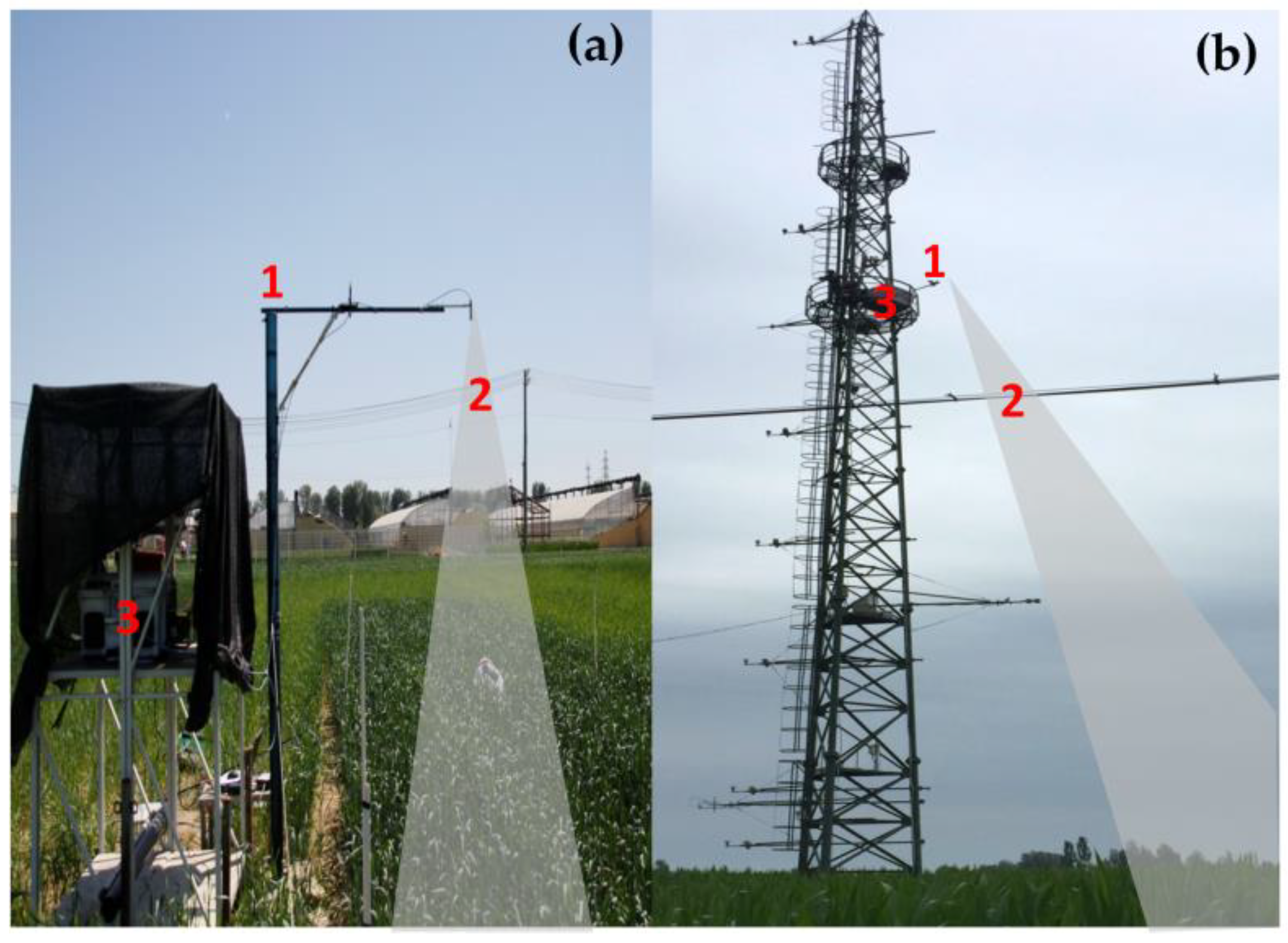
2.1. Tower-Based Measurements

2.1.1. Site Descriptions

Two field sites in China were selected: the Xiaotangshan (XTS) and Daman (DM) sites (

Table 1. Site descriptions and details of the measured height and time window.

Site	Position	Vegetation Type	Measured Height (m)			Time Window
			SIF	Flux	Meteorology	SIF	Flux	Meteorology
XTS	116.44°E 40.18°N	Wheat, C3	3	3	3	2017: 4/30–5/28	/	2017
						2018: 4/10–5/21		2018
DM	100.37°E 38.86°N	Maize, C4	20	5	5	2017: 6/9–9/20	2017	2017

). The XTS site was located in an open and flat area, with a homogeneous wheat cropland, at the National Precision Agriculture Demonstration Base in the town of Xiaotangshan, Beijing. The Daman superstation was located in the Daman irrigation district in the middle reaches of the Heihe River Basin, which is a typical oasis with very flat terrain, approximately 8 km southwest of Zhangye City in northwest China [34]. The dominant plant type grown at the DM site was single-crop maize, which was sown in early May and harvested in mid-September. The main plant type grown at the XTS site was winter wheat, which was sown in late October and harvested in mid-June. Conventional fertilizer and irrigation management were used on these crops, which had a uniform growth status.

Two tower-based systems combining continuous meteorology, flux, and SIF measurements were deployed at the two sites. Table 1 lists the details of the measured height (denoted as the height above canopy) and time window for the SIF, flux, and meteorological measurements. During the wheat and maize growing seasons in 2017 and 2018, synchronous SIF, flux, and meteorological measurements were completed, except for the absence of correct flux data at XTS due to an operating error in the EC system. Although the flux and SIF may be measured with different footprints on the ground, the EC measurements can be representative of a homogeneous cropland at these sites.

2.1.2. Solar-Induced Fluorescence Measurements

An automatically long-term SIF observation system (AutoSIF) was designed and deployed on the platforms of the towers at the two sites for long time series SIF measurements (Figure 2). This system was included in the ChinaSpec network [35], which links in situ spectral measurements with point EC observations for a better understanding of the atmosphere-biosphere interaction. The AutoSIF operating height and time window are listed in Table 1. This system was designed similarly to state-of-the-art systems around the world (e.g., the FluoSpec [21] and Piccolo systems [36]), which are all based on a dual field-of-view (FOV) and hemispherical-conical configuration (for a review, see Reference [37]). The main components integrated in AutoSIF include a customized Ocean Optics QE65PRO spectrometer (Ocean Optics, Dunedin, FL, USA), with a spectral resolution of ~0.3 nm and a signal-to-noise ratio (SNR) higher than 1000 in the range of 645–805 nm, a bifurcated optical fiber (CPATCH, Ocean Optics, Inc., Dunedin, FL, USA), two optical shutters (FOS-1X1-TTL, Ocean Optics, Inc., Dunedin, FL, USA), an automatic refrigeration system, and a controller PC for data collection and storage. The spectrometer was connected to a bifurcated optical fiber with two optical shutters to split the optical signal into two channels: One channel pointing at the zenith, with a cosine corrector (CC3-3-UV-S, Ocean Optics, Inc., Dunedin, FL, USA) to capture downwelling incident radiance from a 180° FOV, and the downlooking channel, which points at nadir or off-nadir with a conical fore-optic (bare fiber) to capture upwelling radiance from a smaller FOV (such as 25°). The two optical shutters separately switched between open and closed to measure the upwelling, downwelling and the systems’ dark current quasi-synchronously.

The measuring mode was a ‘sandwich’ type: First, collect the solar irradiance by opening the shutter of the downwelling channel; second, collect the canopy reflected radiance by opening the shutter of the upwelling channel; finally, measure the solar irradiance again. With immediate channel switching, the system presents a relatively low time delay between up- and downwelling measurements (several seconds). We calculated the average of the two solar irradiance measurements to decrease the effects of weather changes caused by the time delay. Before each of the three single measurements, the integrated time (0.7–6 s) was optimized depending on the light intensity, and the corresponding dark current was measured and finally corrected from the total signal. Generally, the system completed a sandwich measurement cycle from 15 s (midday) to 2 min (sunrise or sunset). The measurement was carried out at a time interval of 2 min. Through the radiometric calibrations, which used a standard calibration light in a darkroom, the digital number (DN) value (with a unit of counts) collected by the spectrometer was converted into radiance (with a unit of mW/m²/nm/sr). Thus, the system automatically and continuously acquired the vegetation-reflected and corresponding solar radiance spectra with high spectral and time resolutions.

The three band Fraunhofer line depth (3FLD) method [38] was used to extract the SIF signal from the measured solar and vegetation-reflected radiances in the atmospheric absorption bands (O₂-A band at approximately 760 nm). This method has been proven to be robust and accurate for SIF retrieval in the O₂-A band (the RRMSE is ~10%) when using spectral measurements via a spectrometer with a spectral resolution of ~0.3 nm and an SNR higher than 1000 [20,39]. The raw SIF data, which were negative or larger than 5 mW/m²/nm/sr, were discarded in the following data process and analysis. For each time period of 30 min (T₃₀), we calculated the half-hour SIF (SIF_T30) by averaging all valid raw SIF measurements (SIF₀) within a time range of 15 min before and after T₃₀:

$${\mathrm{SIF}}_{\mathrm{T}30}={\displaystyle \sum }_{T_{30}-15\min }^{T_{30}+15\min }{\mathrm{SIF}}_0\left(\mathrm{t}\right)/N$$

(1)

where N represents the number of SIF measurements for half an hour. SIF_daily was calculated by integrating the SIF from sunrise to sunset for one day, as shown in Equation (2). The diurnal SZA values at the two sites were calculated using a function that includes latitude (lat), longitude (lon), date, and local time of day (t): $f\left(lat,lon, date, t\right)$. The times of sunrise ($T_{sunrise}$) and sunset ($T_{sunset}$) were determined according to an SZA of less than 90°. Setting the temporal interval at 30 min ($\mathsf{\Delta }{t}_{30}$), the summation form of SIF_daily can be expressed as follows:

$${\mathrm{SIF}}_{\mathrm{daily}}={\int }_{T_{sunrise}}^{T_{sunset}}\mathrm{SIF}\left(\mathrm{t}\right)dt\approx {\sum }_{T_{sunrise}}^{T_{sunset}}{\mathrm{SIF}}_{\mathrm{T}30}\left(\mathrm{t}\right)\times \mathsf{\Delta }{t}_{30}.$$

(2)

During the operating time window of AutoSIF, as listed in Table 1, on 17 and 20 June, 7 and 22 and 12–20 July, 22–31 August, and 1–5 and 7–8 September 2017, at the DM site, spectral measurements failed due to power outages. As a result, we acquired the continuous solar irradiance, vegetation-reflected radiance spectra, SIF_T30 and SIF_daily for 71 and 72 days at the XTS and DM sites, respectively.

2.1.3. Meteorological and Flux Observations

The meteorological and flux variables were observed using an automatic weather station (AWS) and EC system [34], which were fixed on the tower approximately 3, 5, and 20 m above the canopy at the XTS and DM sites. The collected meteorological variables involved in this study included PAR, broadband incoming shortwave radiation (R_in), air temperature (Ta), air pressure (p), wind speed (u), vapor pressure deficit (VPD), and air humidity (Rh). These data were measured and recorded every 10 min with a CR1000 unit (Campbell Scientific Inc., Logan, UT, USA). Similar to the calculation of ${\mathrm{SIF}}_{\mathrm{T}30}$ in Equation (1), PAR and all other meteorological variables were averaged into 30 min intervals to correspond to the flux and SIF observations.

Near the AWS, an EC system was deployed to measure the exchange of energy, water, and CO₂ across the canopy-atmosphere interface. The AWS included a 3D sonic anemometer (CSAT3, Campbell Scientific Inc., Logan, UT, USA) for measuring three-dimensional velocity and temperature and an open-path infrared gas analyzer (Li-7500, Li-Cor, Lincoln, NE, USA) for measuring CO₂ and H₂O density. The main output parameters involved in this study include the net ecosystem exchange of CO₂ flux (NEE), latent heat flux (LE), sensible heat flux (H), friction velocity (u*), and atmospheric CO₂ concentration (Ca). The data were stored in a CR3000 data logger (Campbell Scientific Inc., Logan, UT, USA) and processed with an average time of 30 min at a sampling frequency of 10 Hz.

The GPP data at 30 min intervals (${\mathrm{GPP}}_{\mathrm{T}30}$) were calculated using the online tool available at the Max Planck Institute for Biogeochemistry (MPI-BGC) website (http://www.bgc-jena.mpg.de/ ~MDIwork/eddyproc/), with input variables including R_in, Ta, u*, rH, LE, and H. Gap filling of the EC and meteorological data was performed with methods similar to those in Reference [40]. Daytime NEE was partitioned into GPP and ecosystem respiration based on the night-time partitioning algorithm [41]. GPP_daily was calculated by integrating the GPP from sunrise to sunset for one day, which was similar to the calculation of SIF_daily in Equation (2), and has a time-integrated unit of gC/m²/d.

2.1.4. Vegetation Indexes and FPAR Estimation

Canopy reflectance in the range from 645 nm to 805 nm was calculated with the measurements of solar irradiance and vegetation-reflected radiance spectra. According to the study of Reference [42], the soil-adjusted vegetation index (SAVI) had a close connection with the leaf area index (LAI) and was insensitive to soil reflectance at a low LAI. In this study, the daily averaged SAVI was adopted to estimate the LAI of the wheat canopy at the XTS site in 2017. The SAVI was defined by Reference [43] as:

$$\mathrm{SAVI}=\left(1+\mathrm{L}\right)·\left({\rho }_{801}-{\rho }_{670}\right)/\left({\rho }_{801}+{\rho }_{670}+\mathrm{L}\right)$$

(3)

where the constant L = 0.5 was adjusted to explain the first-order soil background variation. The reflectance at 801 nm was replaced by reflectance at 795 nm in this study due to the limitation in the spectrometer’s wavelength range.

The normalized difference vegetation index (NDVI) was used to estimate the diurnal FPAR. According to previous studies [44,45], for a fixed observed geometry, the diurnal cycles of NDVI and FPAR had similar responses and the FPAR-NDVI relationship was relatively invariant to the SZA. The NDVI was defined as [46]:

$$\mathrm{NDVI}=\left({\rho }_{801}-{\rho }_{670}\right)/\left({\rho }_{801}+{\rho }_{670}\right).$$

(4)

Similarly, we used reflectance at 795 nm instead of 801 nm in this study. Based on the NDVI linear stretching model reported in Reference [47] and Reference [48], the diurnal FPAR can be expressed as:

$$\mathrm{FPAR}=\frac{\mathrm{NDVI}-{\mathrm{NDVI}}_{\min }}{{\mathrm{NDVI}}_{\max }-{\mathrm{NDVI}}_{\min }}·({\mathrm{FPAR}}_{\max }-{\mathrm{FPAR}}_{\min })$$

(5)

where ${\mathrm{NDVI}}_{\min }$ and ${\mathrm{NDVI}}_{\max }$ were set at 0.3 and 0.925 for the crops in our study area and, generally, ${\mathrm{FPAR}}_{\min }$ and ${\mathrm{FPAR}}_{\max }$ were 0.001 and 0.95, respectively [47]. Liu [19] compared the model-predicted FPAR with the measured FPAR data and demonstrated that this NDVI-based model reliably estimated FPAR and its diurnal variations. Then, the diurnal FPAR values for all measuring days were estimated using the measured spectral data. Accordingly, the absorbed PAR (APAR) values were calculated as the product of FPAR and PAR derived by the AWS. Similar to the calculation of ${\mathrm{SIF}}_{\mathrm{T}30}$ in Equation (1), half-hour APAR data (${\mathrm{APAR}}_{\mathrm{T}30}$) were derived. The daily APAR (${\mathrm{APAR}}_{\mathrm{daily}}$) was calculated by integrating the APAR from sunrise to sunset for one day, which was similar to the calculation of SIF_daily in Equation (2) and has a time-integrated unit of MJ/m²/d.

2.2. GPP from SCOPE Model Simulations

Considering the absence of GPP data at XTS in 2017 and 2018 (the EC system was not operating properly, and the flux data were incorrect), we used the Soil-Canopy Observation of Photosynthesis and Energy (SCOPE) model v1.61 [49] to simulate GPP at 30 min intervals to relate the measured SIF data. According to the global sensitivity analysis (GSA) of the SCOPE model in Reference [50], apart from the meteorological inputs, the chlorophyll content density (Cab), LAI, and maximum carboxylation rate (V_cmax) were the main driving variables that governed the simulated SIF and likely the GPP. For GPP simulation at XTS in 2018, the input vegetation parameters, including Cab and LAI, were measured from field experiments at 6–10 days intervals, as listed in

Table 2. The input chlorophyll content density (Cab) (unit: μg/cm²), leaf area index (LAI), and maximum carboxylation rate (V_cmax) (unit: μmol/m²/s) values for the gross primary productivity (GPP) simulation of the Soil-Canopy Observation of Photosynthesis and Energy (SCOPE) model during the time window of the SIF measurements in 2017 and 2018.

	2017						2018
	4/29	5/9	5/19	5/24	5/28	6/1	4/9	4/16	4/24	5/3	5/13	5/23	5/31
Cab	65	65	60	55	30	20	47.5	47.4	58.4	63.4	65.1	59.8	33.6
LAI	2.10	2.00	1.91	1.81	1.52	0.75	1.09	1.57	1.71	2.28	1.77	1.64	1.03
Vcmax	110	90	80	70	55	40	50	60	70	110	90	70	50

. Cab was determined using measurements from a SPAD-502 (Soil and Plant Analyzer Development) chlorophyll meter [51], and the LAI was measured by the scanning method. For simulation at XTS in 2017, daily LAI was estimated with the SAVI-LAI linear model that derived from the measurements in 2018; then, Cab was retrieved with the model inverting method similar to Reference [52]. More specifically, daily Cab was estimated by minimizing the difference between the measured and SCOPE-simulated reflectance spectra in the region at 650–750 nm, with a lookup table (LUT) of input Cab values from 20 to 70 μg/cm² and a step of 5 μg/cm².

V_cmax can be estimated from net CO₂ flux measurements by inverting the commonly used modeling paradigm of canopy CO₂ and energy fluxes [53]. Based on this method and using the SCOPE model, our previous study [54] successfully estimated the V_cmax values throughout the growing season of wheat at XTS in 2015 and 2016. The estimated V_cmax values between the two years had consistent seasonal values, with a range of 30–110 μmol/m²/s. According to a previous study [55], during the crop’s growing season, V_cmax increased rapidly with time until it reached its maximum during the mid-growing season and then declined toward the end of the growing season. Based on this prior knowledge and considering that wheat has a similar growth status between adjacent years under conventional fertilizer and irrigation management, the V_cmax values on different days of the year in 2017 and 2018 were set as their values on corresponding days of the year in 2015 and 2016. Table 2 lists the retrieved or measured Cab, LAI, and V_cmax values for the model inputs during the time window of the SIF measurements at 4–10 days intervals.

Meteorological variables that control the variations in GPP simulations (i.e., R_in, Ta, p, u, and VPD) were derived from the AWS observations. All half-hour meteorological variables and seasonally changed inputs (including Cab, LAI, and V_cmax, as shown in Table 2) were imported into the model input files and loaded for the time series simulations of GPP with SCOPE. Meanwhile, the diurnal SZAs were automatically calculated during the simulation using the inputs Julian day, time, and field site longitude and latitude. Other parameters required by the SCOPE model were set to their default values for each plant functional type (for details, see Reference [50]). With all of these directly measured or indirectly retrieved inputs, the SCOPE model accurately interpreted the diurnal and seasonally changed values of the GPP.

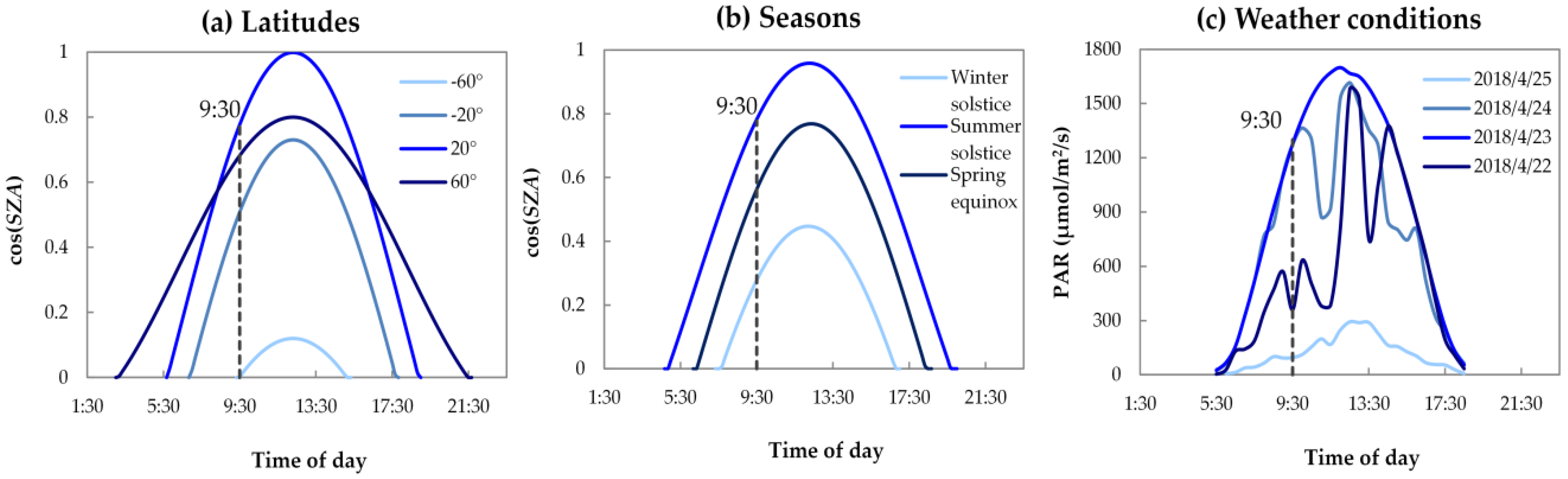
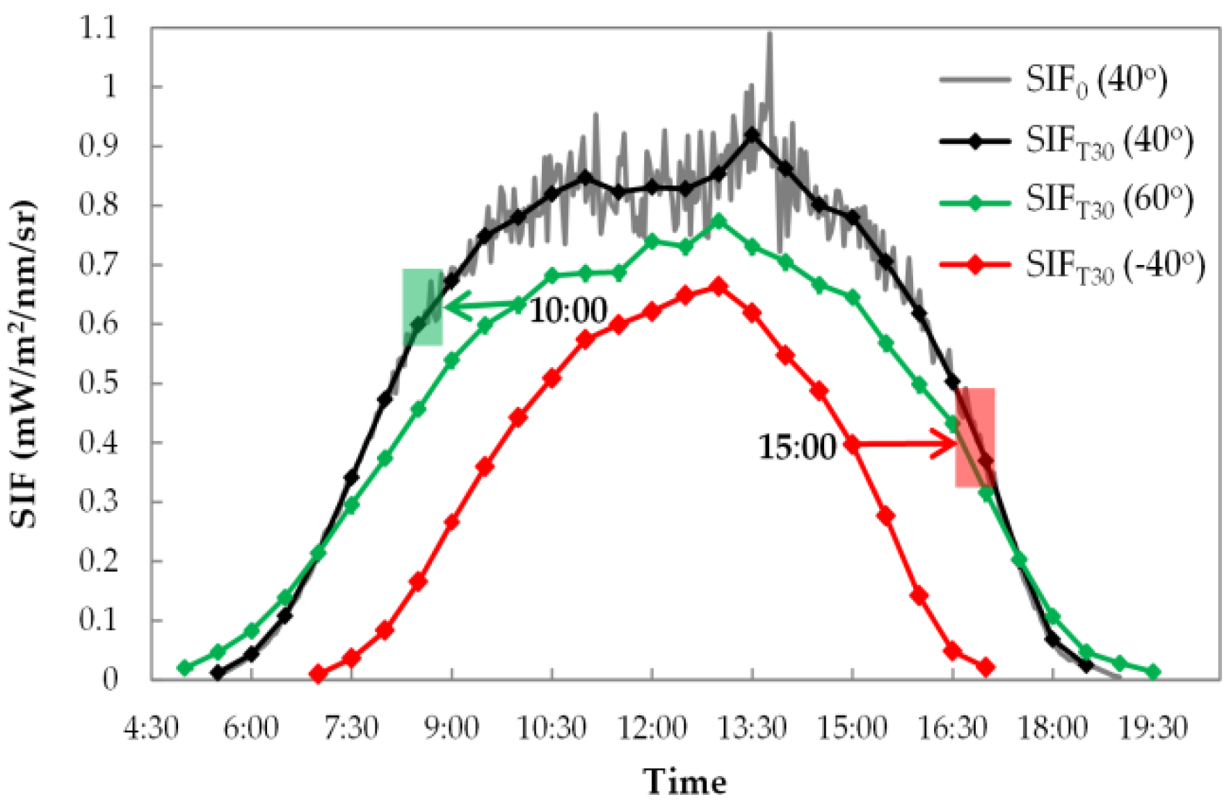
2.3. Simulating SIF and APAR at Different Latitudes

Remote sensing often observes ground features across different latitudes that receive changed levels of solar radiation. The latitudinal pattern of incoming solar radiation causes large uncertainties in the application of remote sensing at the global scale. For the SIF_inst observation, latitude is a large factor that affects the relationships between SIF_inst and SIF_daily (see Figure 1a) and, thus, may affect the performance of SIF for the APAR or GPP estimation. However, this study only obtained data from two sites distributed at similar latitudes, which was insufficient for the investigation of SIF applications at different latitudes. To better understand the latitudinal effects on the SIF-APAR relationship, we used the SIF, PAR, and FPAR measurements at limited sites with a latitude of ~40° to simulate their corresponding values at other latitudes. As the latitudinal patterns of incoming solar radiation were only attributed to the latitudinal variations in SZA, it was reasonable to neglect the weather changes among different latitudes and, thus, to simulate PAR values at different latitudes based on the latitudinal SZA changes. Similarly, based on the assumptions that the crop growth status and plant physiological response to illumination are the same across latitudes, the SIF, FPAR, and thus APAR values at these latitudes can be simulated. The spatial heterogeneities of environmental conditions (e.g., weather, temperature, and precipitation), soil types, plant varieties, and vegetation growth status were not taken into consideration because they were irrelevant to the analysis of latitudinal variations in SIF-APAR relationships.

In this study, we picked three different latitudes, including −20°, −40°, and 60°, to perform simulations based on the measurements at each of the two sites. These latitudes were selected because they are spatially representative and the minimum SZA values at these latitudes were lower than the minimum SZA values at a latitude of 40° during our measuring period. Figure 3 displays an example of the simulation of SIF at different latitudes. Using the diurnal SIF measurements at a latitude of 40° (gray line in Figure 3), the diurnal SIF values on the same day at other latitudes (green and red lines in Figure 3) were calculated based on the latitude-dependent SZA values. Specifically, the SIF value of time t1 at a latitude of 60° or −40° equaled the SIF value of time t2 at a latitude of 40°, where t1 and t2 correspond to the same SZA and both occur in the morning or afternoon. For instance, the SIF_T30 value at 10:00 at a latitude of 60° (see the green arrow in Figure 3) can be simulated as follows: (1) calculate the range of SZA (ΔSZA) corresponding to the time range [9:45 10:15] at a latitude of 60°, (2) search for the set of SIF₀ measurements at a latitude of 40° in the morning that satisfy the condition where their corresponding SZA values are within ΔSZA (the green frame in Figure 3), and (3) average the searched SIF set in the previous step as the SIF value at 10:00 at a latitude of 60°. The simulation of the SIF_T30 value at 15:00 at a latitude of −40° (see the red arrow in Figure 3) was similar but the searched time window was in the afternoon. By repeating these steps for each half-hour time for all days and other latitudes, 12 time series of continuous SIF, PAR, and APAR datasets at 30 min intervals were generated at four different latitudes at two sites.

2.4. Temporal Upscaling from Instantaneous to Daily SIF

SIF can be expressed as a product of PAR, FPAR, and the quantum yield for fluorescence (${\mathrm{LUE}}_{\mathrm{f}}$), given that $f_{esc}$ is almost constant for a given vegetation species [16]. As ${\mathrm{LUE}}_{\mathrm{f}}$ and FPAR have much smaller diurnal variations compared to the diurnal variation in PAR [19,27], the SIF was regarded as approximately linear related to the PAR at a diurnal scale. Several studies have also demonstrated that there is a significant linear correlation between the SIF and PAR at the diurnal scale using in situ measurements [17,20,28,29]. Therefore, the SIF value at any time of a day can be approximately calculated using the ratio of SIF to PAR for a given instantaneous time and with continuous diurnal PAR data, which is expressed as:

$$\mathrm{SIF}\left(\mathrm{t}\right)\approx \frac{{\mathrm{SIF}}_{\mathrm{inst}}}{{\mathrm{PAR}}_{\mathrm{inst}}}·\mathrm{PAR}\left(\mathrm{t}\right).$$

(6)

By integrating $\mathrm{SIF}\left(\mathrm{t}\right)$ with time from sunrise to sunset over one day, the daily integrated SIF can be approximately calculated as follows:

$${\mathrm{SIF}}_{\mathrm{daily}}\approx {\mathrm{SIF}}_{\mathrm{inst}}·\frac{{\mathrm{PAR}}_{\mathrm{daily}}}{{\mathrm{PAR}}_{\mathrm{inst}}}$$

(7)

where ${\mathrm{PAR}}_{\mathrm{daily}}$ was calculated by integrating the half-hour PAR from sunrise to sunset for one day, which was similar to the calculation of SIF_daily in Equation (2) and had a time-integrated unit of MJ/m²/d. ${\mathrm{PAR}}_{\mathrm{daily}}/{\mathrm{PAR}}_{\mathrm{inst}}$ can be regarded as the temporal conversion factor from ${\mathrm{SIF}}_{\mathrm{inst}}$ (mW/m²/nm/sr) to ${\mathrm{SIF}}_{\mathrm{daily}}$ (J/m²/nm/sr/d).

Recent studies (e.g., References [14,27,31]) used an approximate clear-sky PAR proxy ($\cos \left(\mathrm{SZA}\right)$) to replace PAR in Equation (7) for SIF upscaling from the instantaneous to daily scale. This cos-based method for SIF temporal upscaling assumes that the diurnal variation in SIF only depends on the SZA values and did not consider cloud and atmospheric scattering effects. In this study, we upscaled SIF_inst at a given time of 9:30 to SIF_daily using these two upscaling methods (i.e., the cos-based and PAR-based methods) with the tower-based measurements at the two sites and then investigated whether the PAR-based SIF_daily can improve the SIF-GPP correlation instead of using SIF_inst or cos-based SIF_daily.

3. Results

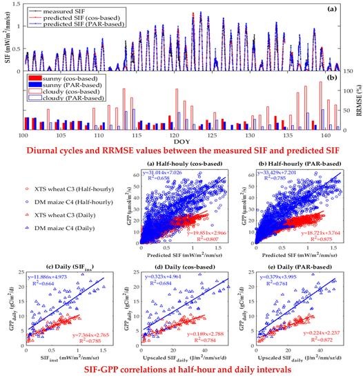
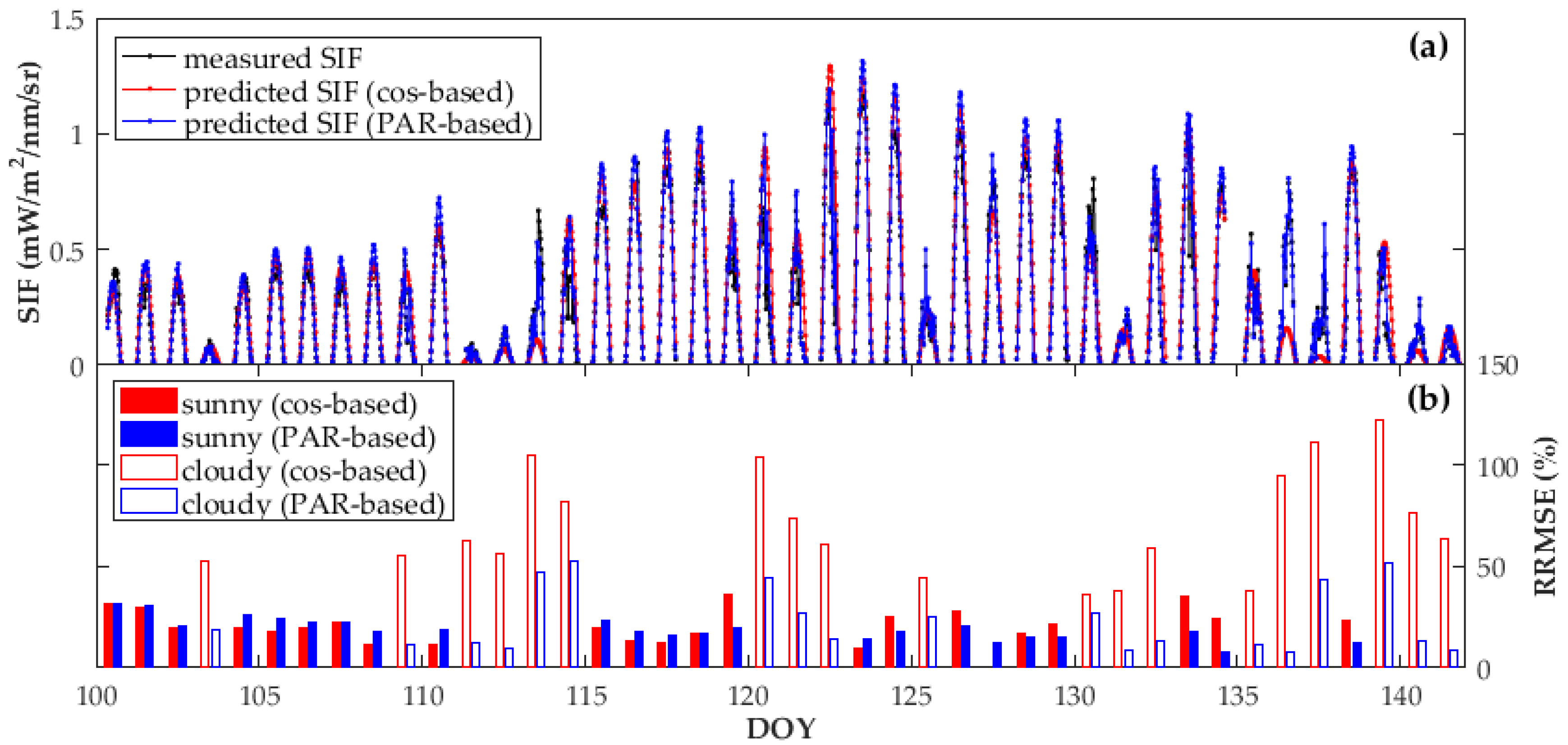
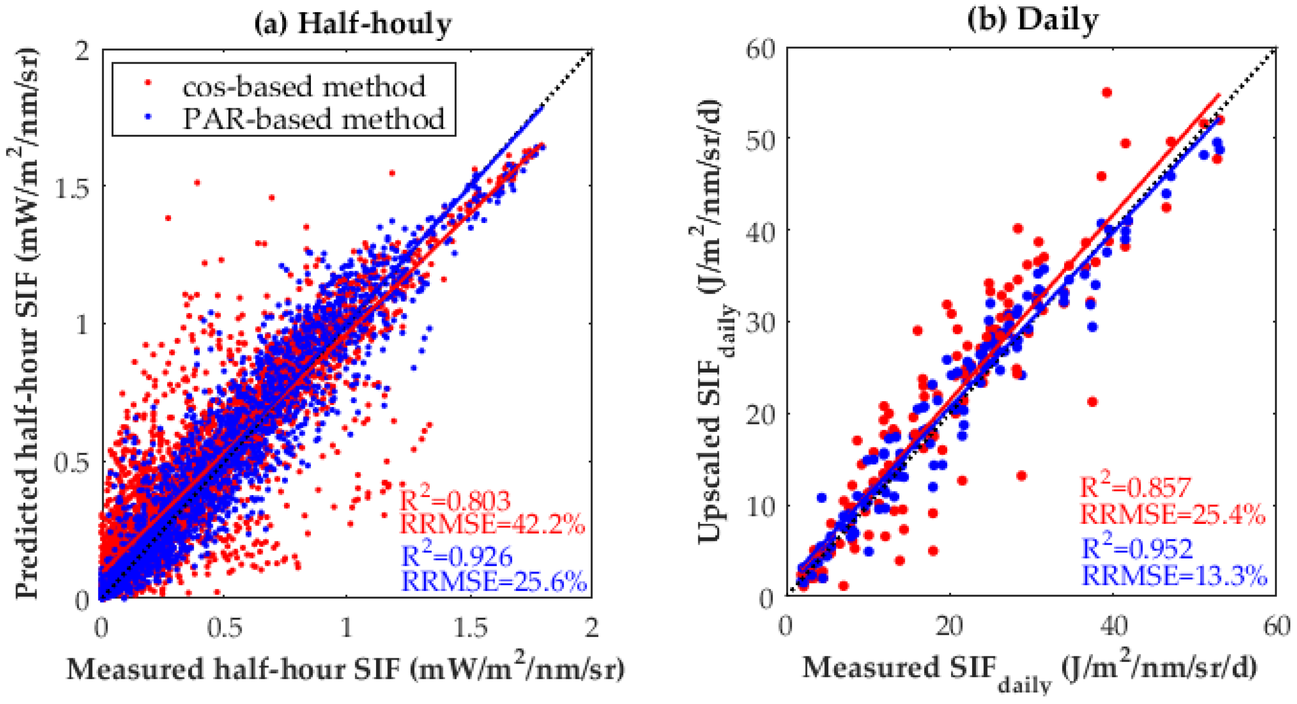
3.1. Evaluating the Accuracy of Upscaled SIF with Long-Term Measurements

To quantitatively assess the accuracies of the PAR-based method and cos-based method for SIF upscaling from the instantaneous to daily scale, the tower-based SIF measurements at the two sites were regarded as the reference data for comparison with the upscaled SIF at half-hour and daily intervals.

First, for each measurement day, we evaluated the accuracy of the predicted SIF_T30 at two sites. The predicted SIF values using the two upscaling methods were compared with the measured SIF values to investigate whether the predicted SIF reliably tracked the diurnal cycles of SIF measurements. We also calculated the corresponding relative root mean square error (RRMSE) values between the measured and predicted SIF values for each day. The measurement days were divided into two weather conditions, sunny and cloudy days, by judging whether the coefficient of determination (R²) between PAR and $\cos \left(\mathrm{SZA}\right)$ was larger than 0.9. Figure 4 displays the results for the XTS site in 2018 as an example. On sunny days with clear sky conditions (labeled with solid bars in Figure 4b), the diurnal SIF values predicted by both methods were quite consistent with the measured SIF values: The RRMSE values of the two methods were comparable and less than 40%. However, on cloudy days with unstable weather conditions (labeled with hollow bars in Figure 4b), only the SIF values predicted by the PAR-based method can reliably track the diurnal cycles of the measured SIF. The RRMSE values of the SIF predicted by the cos-based method were larger than 60% for most cloudy days due to the effects of clouds and scattering light.

Secondly, for all measurement days, we evaluated the accuracy of the predicted SIF at the two sites at both half-hour and daily intervals. Figure 5 shows the correlation analysis between the predicted SIF using the PAR-based and cos-based methods with the measured SIF at the two sites at two temporal scales: half-hour and daily. In general, the predicted SIF values using the PAR-based method at both half-hour and daily temporal scales match the reference values well: The points were located close to the 1:1 line, the R² values were higher than 0.9, and the RRMSE values were 25.6% at the half-hour interval and 13.3% at the daily interval. However, the predicted SIF values using the cos-based method were not as robust as those predicted by the PAR-based method, with significantly lower R² values and larger RRMSE values at both half-hour and daily intervals.

From the accuracy assessment on SIF upscaling for both individual days and all measuring days, we can conclude that the PAR-based method can predict diurnal and SIF_daily more accurately than the cos-based method. The main reason for this lies in the effects of large weather changes on cloudy days. For more accurate SIF upscaling from the instantaneous to daily scale, the diurnal changes in weather should be taken into account by integrating the continuous PAR data for SIF upscaling.

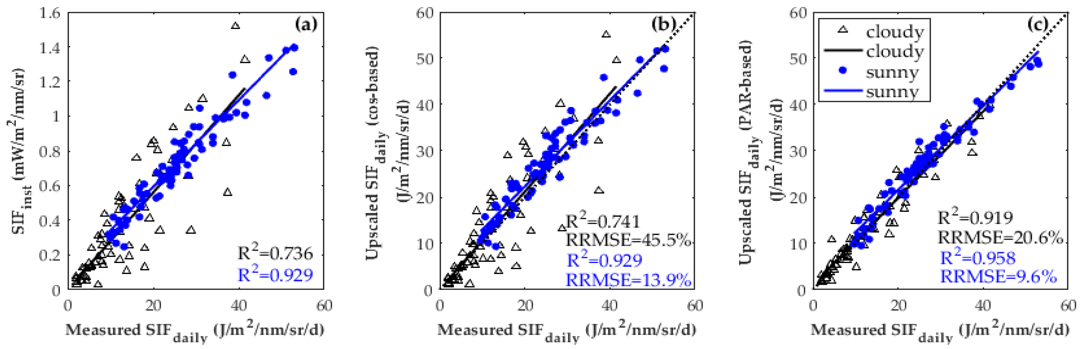
3.2. Comparison between Instantaneous SIF and Daily SIF Across Space and Time

To investigate whether the upscaled SIF_daily can reduce the variations in the SIF_ins-SIF_daily correlation across space and time, we compared SIF_ins (at 9:30) and the upscaled SIF_daily using two upscaling methods (i.e., the cos-based and PAR-based methods) with the measured SIF_daily under different weather conditions and different latitudes (simulated data).

Figure 6 displays the correlations between SIF_ins and upscaled SIF_daily with the measured SIF_daily for sunny and cloudy days at the two sites. On sunny days (labeled with blue symbols in Figure 6), the SIF_ins-SIF_daily correlations for different days were relatively stable, with R² values larger than 0.9. In this case, the relevance of the measured SIF_daily with upscaled SIF_daily was similar to that with SIF_inst: the R² values for the three kinds of SIF were basically the same and the RRMSE values for SIF_daily using the two upscaling methods were comparable and both less than 15%. On cloudy days (labeled with black symbols in Figure 6), the SIF_ins-SIF_daily correlations changed remarkably across different days; R² was approximately 0.7. Note that these variations can only be reduced by upscaling SIF_inst using the PAR-based method; R² for the PAR-based upscaled SIF_daily was significantly larger than that for SIF_inst. However, upscaling SIF_inst using the cos-based method made no improvement for the SIF_ins-SIF_daily correlation on cloudy days; R² for this method was almost equal to that for SIF_inst, and the corresponding RRMSE value was significantly greater than that for the PAR-based method.

Apart from weather conditions, latitudes were also an influential factor on the variations in SIF_ins-SIF_daily correlations across space and time (see Figure 1). Figure 7 displays the correlations between SIF_ins and upscaled SIF_daily with the measured SIF_daily for four different latitudes simulated using the observations at the XTS and DM sites. Considering that the R² value of the regression without an intercept is very close to that with an intercept, we conducted the regression with a zero intercept to better compare the slopes of the SIF_ins-SIF_daily correlations among the four latitudes. The corresponding R² values and coefficient of variation (CV) of the regression slopes for the four latitudes were also calculated. The variations in the SIF_ins-SIF_daily correlations across different latitudes can be significantly reduced by upscaling the SIF_inst to a daily scale using both the cos-based and PAR-based methods. Specifically, the regression slopes for the upscaled SIF_daily exhibited substantially smaller variations than those for the SIF_inst (CV = 0.034 for the cos-based method). For the PAR-based method, the regression slopes tended to be normalized at a constant value, with a CV of 0.01. However, for individual latitudes, only the PAR-based method corrected the influence of weather conditions on the SIF_ins-SIF_daily correlations, with impressively larger R² values than those of the SIF_inst but the cos-based method did not achieve this effect with nearly the same R² values as those for the SIF_inst. It results in a relatively lower increase in R² for the SIF_ins-SIF_daily overall correlation across all latitudes when using the cos-based method (increasing the value of R² from 0.789 to 0.842) than that when using the PAR-based method (increasing the value of R² from 0.789 to 0.942).

In view of the above results, latitude and weather conditions were two important factors affecting the variations in SIF_inst-SIF_daily correlations and, thus, the SIF-APAR and SIF-GPP relationships across space and time, respectively. The effects of latitude can be reduced by upscaling SIF_inst to a daily scale using the cos-based method, whereas the effects of weather conditions cannot be corrected by this method due to clouds or scattered lights. SIF_inst may not be a substitute for SIF_daily when assessing the SIF-GPP relationship across space and time unless considering both latitudinal and diurnal weather changes via SIF upscaling using the PAR-based method.

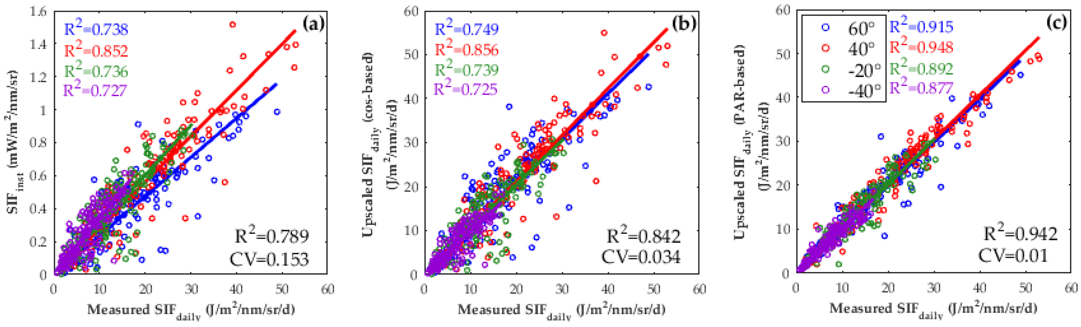
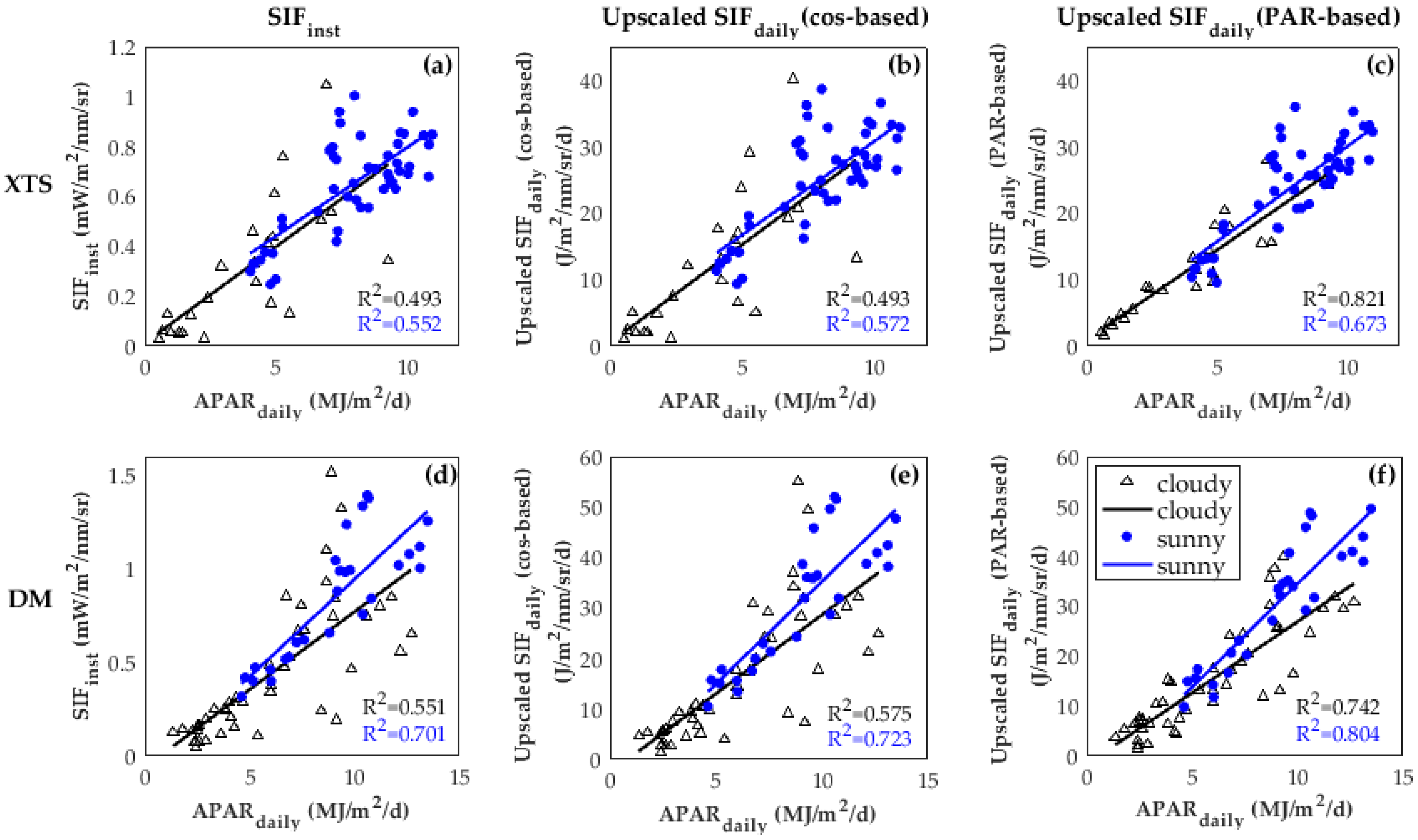
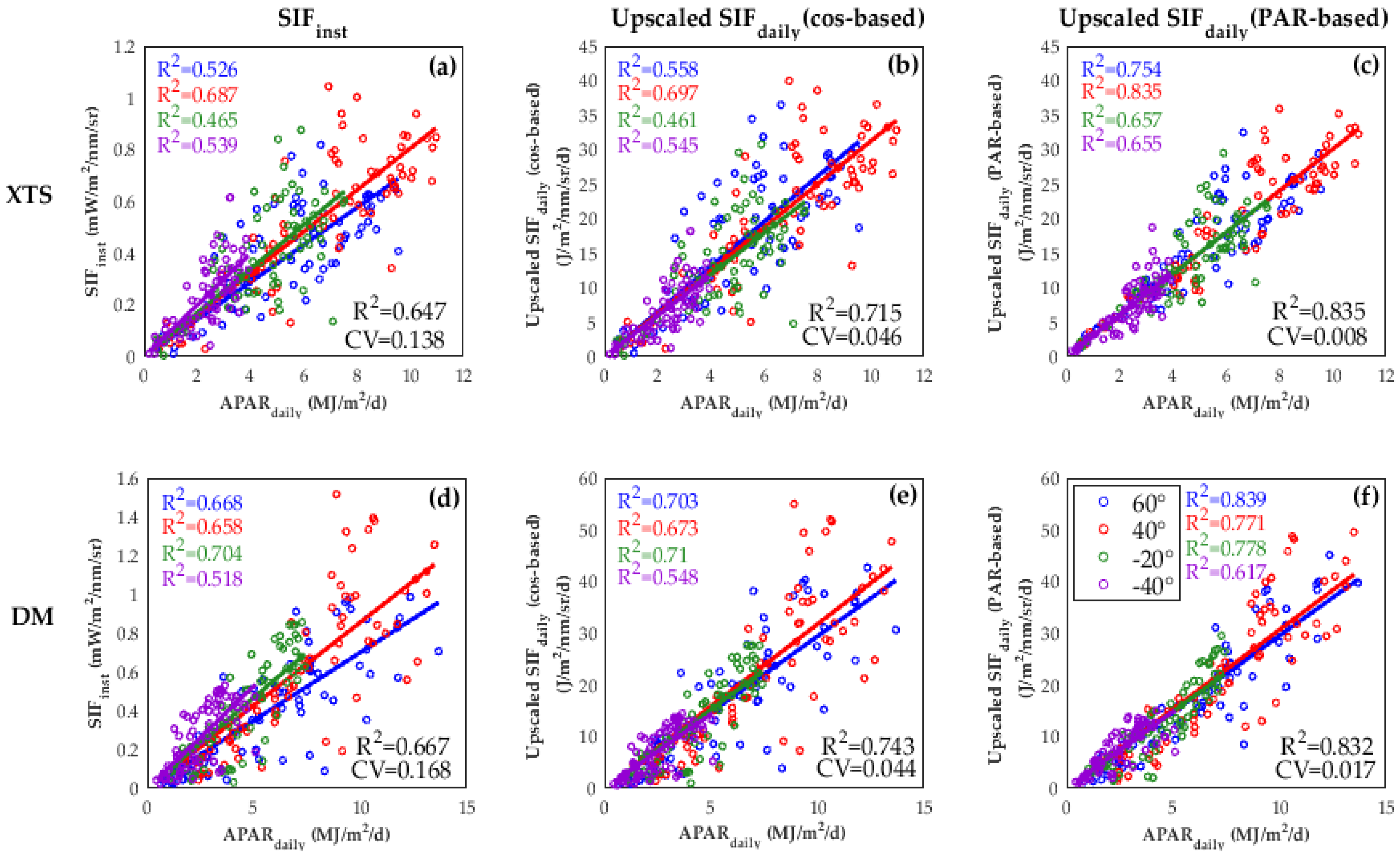
3.3. Comparison between SIF and APAR Across Space and Time

The SIF_inst-SIF_daily correlations changed substantially with different latitudes and weather conditions. How does this result affect the relationship between SIF and APAR or GPP? whether the SIF-APAR or SIF-GPP relationships via SIF upscaling from instantaneous to daily scales should be further verified. APAR is a bridge that links SIF to GPP [11,13,30] and has been proven to dominate the SIF-GPP relationship [56]. Therefore, the investigation of SIF-APAR correlations across space and time is required to better understand the SIF-GPP relationships, which is demonstrated as follows.

Figure 8 shows the correlations between APAR_daily with the SIF_ins and upscaled SIF_daily, using the two methods for sunny and cloudy days at the XTS and DM sites. Similar to the correlations shown in Figure 6, at both sites on sunny days, the R² values for the three kinds of SIF all exhibit weak changes, whereas, on cloudy days, the R² values can be greatly increased when comparing APAR_daily with PAR-based SIF_daily instead of SIF_ins or cos-based SIF_daily. Figure 9 reports the correlations between SIF_ins and the upscaled SIF_daily with APAR_daily for four different latitudes simulated using observations at the XTS and DM sites. The large variations in the regression slopes for SIF_ins-APAR_daily across different latitudes could be reduced by SIF upscaling at both sites, especially when using the PAR-based method, which was also similar to the correlations shown in Figure 7.

In conclusion, the variations in the SIF_inst-SIF_daily correlations are important reasons for the changes in the SIF-APAR relationship across space and time. At the spatial scale, the SIF-APAR relationship was impacted when using SIF_inst due to the effect of different latitudes. At the temporal scale, the SIF-APAR relationship had uncertainties when using both SIF_ins and cos-based SIF_daily due to the effect of different weather conditions. Both of these effects can be reduced and, thus, the SIF-APAR relationship across space and time can be effectively improved by upscaling SIF_inst to a daily scale using the PAR-based method.

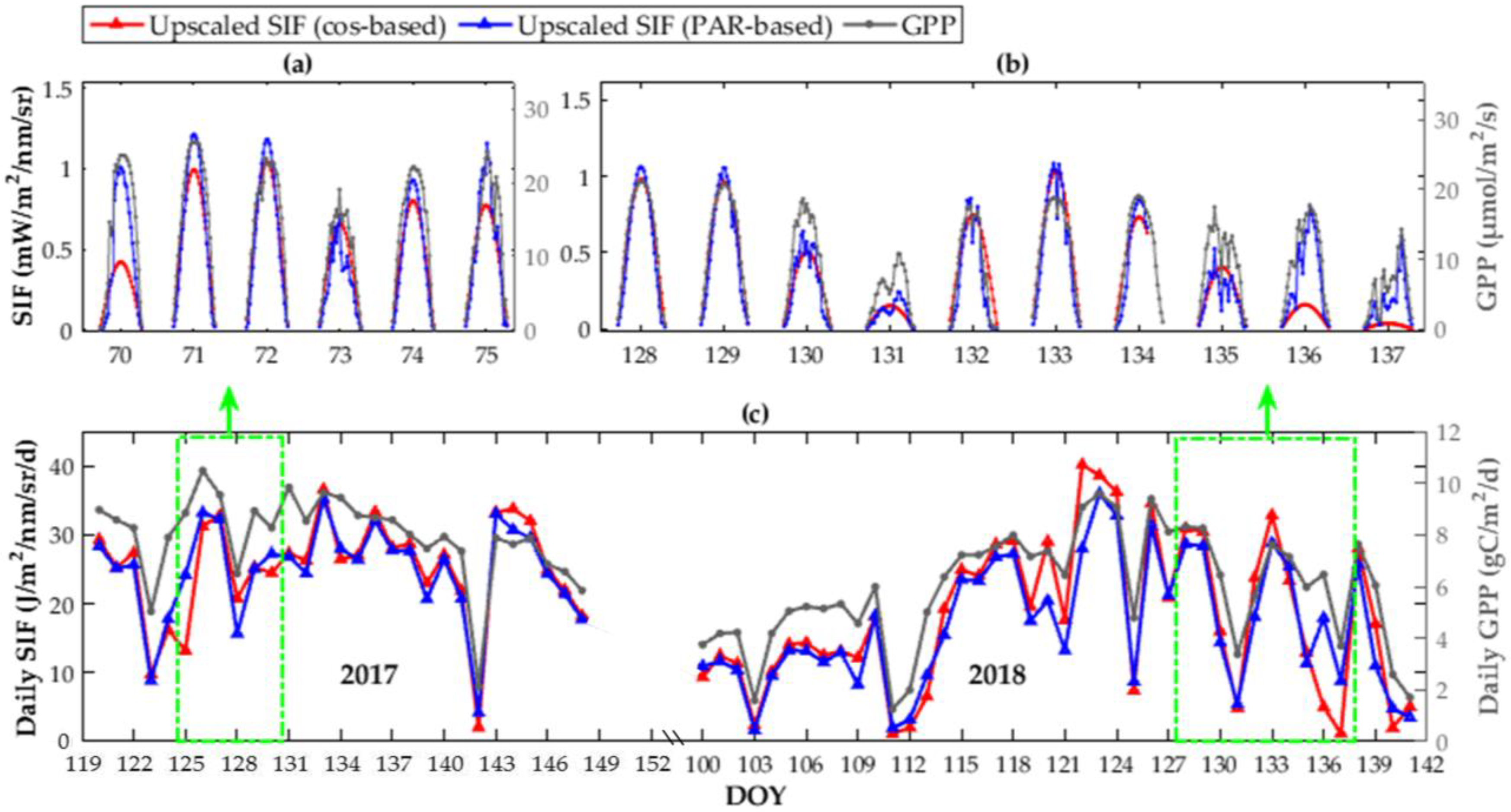
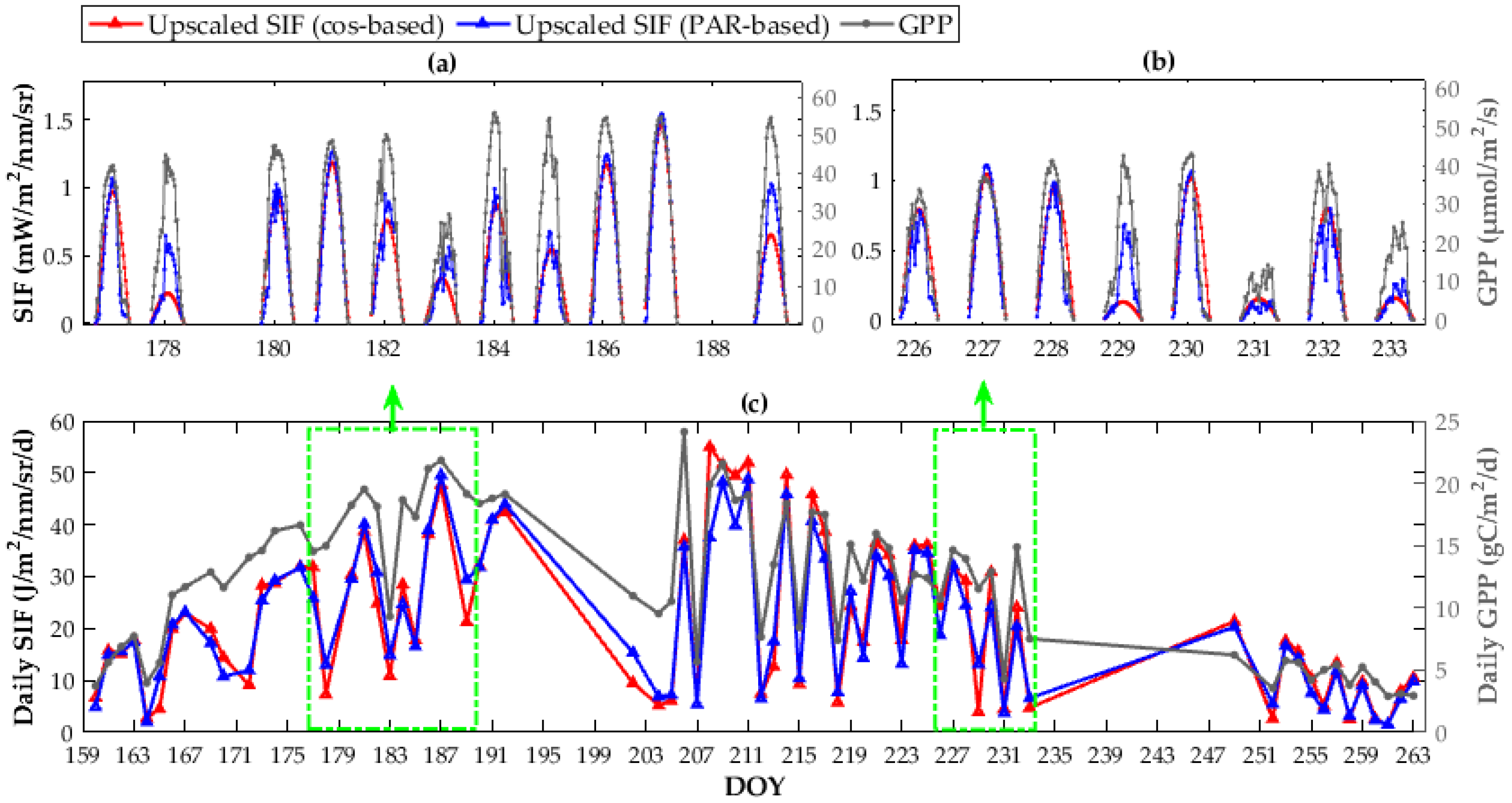
3.4. Performance of Upscaled Daily SIF to Track GPP at the Seasonal Scale

As demonstrated above, the effects of changed weather conditions on the differences between the instantaneous scale and daily scale can be reduced by upscaling SIF_inst to the daily scale using PAR data. As the GPP is a product of APAR and LUE, the improvement in the SIF-APAR relationship caused by SIF upscaling using the PAR-based method may produce a better correlation between GPP_daily and SIF.

Figure 10 and Figure 11 display the seasonal cycles of GPP_daily and upscaled SIF_daily, respectively, using two methods at the XTS and DM sites. To obtain a better understanding, the SIF_T30 and GPP data on some representative days are emphatically shown in the figures. We did not exhibit the seasonal cycles of the SIF_inst values because they were almost the same as those of the cos-based upscaled SIF_daily. In general, the upscaled SIF_daily using both methods can reliably track the seasonal changes in GPP_daily at the two sites. Specifically, the GPP_daily and upscaled SIF_daily using the two methods all exhibit similar seasonal cycles across the growth seasons for wheat and maize; they all increase at first with crop revival and growth and then decrease with the crop senescence. However, for several days that experienced substantial changes in weather (e.g., the 125th day in 2017 and the 136th and 137th days in 2018 at the XTS site (see Figure 10) and the 178th, 183th, 229th, and 230th days at the DM site (see Figure 11)), the diurnal cycles of the PAR-based SIF agreed better with the diurnal GPP changes and, thus, the PAR-based upscaled SIF_daily values were more accurate than the cos-based upscaled SIF_daily. This result made the seasonal cycles of PAR-based upscaled SIF_daily more consistent with the seasonal GPP_daily than the cos-based upscaled SIF_daily. Note that both the upscaled SIF_daily by the two methods and the measured SIF_daily will underestimate GPP_daily on those cloudy days (see Figure 10 and Figure 11), especially for the data at the DM site.

Figure 12 reports the quantitative assessment of the SIF-GPP correlations at half-hour and daily intervals for C3 and C4 crops at the XTS and DM sites, respectively. At the half-hour interval, the predicted SIF using the PAR-based method has a stronger correlation with the GPP than that using the cos-based method, with an increasing R² from 0.658 to 0.785 at the DM site and from 0.807 to 0.875 at the XTS site. More importantly, at daily intervals, the upscaled SIF_daily using the PAR-based method also had an obviously stronger correlation with GPP_daily than with SIF_inst or the cos-based SIF_daily; the R² values increased from approximately 0.68 to 0.76 at the DM site and from approximately 0.78 to 0.87 at the XTS site. However, the cos-based method did not reduce the differences between SIF_inst and SIF_daily at the seasonal scale, with nearly the same R² values as those for SIF_inst. Note that the higher R² values of the SIF-GPP correlation at the XTS site than those at the DM site were caused by the simulated GPP at the XTS site as opposed to the measured GPP at the DM site, which was independent of the different vegetation functional types for the C3 and C4 crops. In conclusion, at the seasonal scale, the SIF-GPP correlations can be obviously improved when comparing the PAR-based SIF_daily with the GPP_daily instead of SIF_inst and the cos-based SIF_daily at both half-hour and daily intervals. This improvement was important for more reliable GPP estimation at the seasonal scale.

4. Discussion

4.1. Prospects of Improving GPP Estimation by SIF Upscaling

Based on the biome-specific SIF-GPP correlations, the space-based SIF has been successfully used to estimate the GPP at global scales [16]. In most studies that link the SIF to GPP, the SIF occurred at an instantaneous scale but the GPP occurs at a time-integrated scale, which caused uncertainties in the SIF-GPP model and, thus, affected the GPP estimation. It has been demonstrated in Reference [27] that upscaling the GOME-2 monthly product from the instantaneous to daily scale can improve its correlation with the monthly GPP product across different biome types because the effects of latitude on SIF_ins-GPP variations have been corrected. Furthermore, this study upscaled the SIF_inst to a daily scale using PAR as a driving variable. Long-term SIF and GPP measurements have validated that this PAR-based method can reduce not only the latitude dependency but also the weather dependency of the SIF-GPP model, which is likely to improve the accuracy of GPP estimation at the ground and spatial scales.

Further opportunities are available to evaluate the advantages of PAR-based SIF upscaling for GPP estimation at a global scale using the space-based SIF product (e.g., the GOME-2 monthly SIF product or the TROPOspheric Monitoring Instrument (TROPOMI) SIF product [57]) and the global PAR and GPP products. To date, most global SIF products are gridded monthly averages of valid SIF observations within one month. As satellites can only derive no more than one SIF observation per day, and valid SIF observations mainly occur on sunny days, the monthly SIF averages cannot represent the real monthly SIF to estimate the monthly GPP due to the contributions of photosynthesis and SIF emissions during cloudy weather conditions. Using continuous PAR data for SIF upscaling may solve this problem. If the effects of FPAR and fluorescence efficiency changes on SIF within one month are neglected, the upscaled monthly SIF can be calculated as a product of the instantaneous mean SIF validly observed at 9:30 (local time) and the ratio of the monthly averaged PAR to the corresponding instantaneous PAR. The calculated results will have an additional error due to neglecting the fluorescence efficiency and FPAR changes. Considering the variations in FPAR and fluorescence efficiency with the vegetation growing in one month, SIF products at higher temporal resolutions (e.g., daily or weekly) can be also derived using the data-driven method by integrating reflectance-based products (reflectance, vegetation index, FPAR) and PAR data. Similar to the approach in the studies of References [58,59], a neural network can first be trained using the instantaneous SIF observations and the instantaneous driven-variables (including PAR, reflectance-based products); then the high-temporal resolution SIF at a daily or weekly resolution can be calculated by using the trained neural network and its key driven variables, including reflectance-based vegetation products (reflectance, vegetation index, FPAR) and the daily or weekly PAR dataset.

4.2. Uncertainty Analysis

Using tower-based spectral measurements combined with flux measurements is an efficient way to investigate SIF upscaling and SIF-GPP links. In this study, the result that upscaling SIF_inst to the daily scale reduces the effects of latitude on the SIF_ins-SIF_daily and SIF_ins-APAR_daily relationships agree with the results of the SIF-GPP correlations in [27]. Therefore, although the SIF and APAR data at different latitudes were obtained from simulations rather than measurements, this does not affect the analysis on the influence of latitude on SIF-GPP variations. In addition, the results of the SIF-GPP correlations indicate that the slope of the GPP–SIF relationship was much higher for C4 crops, which is consistent with the results in [19], demonstrating that this phenomenon is due to similar fluorescence efficiency but a large difference in LUE between C3 and C4 crops.

There are some uncertainties and limitations in this study. First, the PAR-based SIF upscaling method considered that the diurnal SIF is only driven by diurnal PAR variations. Although diurnal variations in FPAR and fluorescence efficiency are much smaller compared to the diurnal variation in PAR, it also affects the diurnal cycles of SIF [20,56] and, thus, brings some errors in the PAR-based predicted SIF values and upscaled SIF_daily. Second, the GPP data at the XTS site were simulated using the SCOPE model by measuring or retrieving the main driving variables (e.g., Cab, LAI, and V_cmax) for GPP simulation. The measuring and retrieving uncertainties bring some errors for the parameterization of the SCOPE model and, thus, for the accuracy of the GPP. More GPP observations corresponding to SIF measurements should be collected to support the results in this study.

5. Conclusions

The temporal mismatch between SIF_inst and GPP_daily causes uncertainties in the spatio-temporal patterns of SIF-GPP correlations; therefore, the upscaling of SIF from the instantaneous to daily scale is important for investigating the link between the SIF and GPP. In this paper, we upscaled the in-situ SIF measurements from an instantaneous to daily scale using the ratio of the PAR_inst to PAR_daily as a temporal conversion factor. With the continuous tower-based spectral observations, combined with meteorological and flux measurements at two sites, the accuracy of the PAR-based method and the performance of upscaled SIF to track GPP were evaluated, which was also compared to the commonly used cos-based upscaled SIF. The conclusions are summarized as follows.

First, the PAR-based method gives more accurate diurnal and SIF_daily predictions than the cos-based method because the PAR-based method considers diurnal weather changes on cloudy days. In addition, the upscaled SIF_daily using the PAR-based method shows a more robust and significant relationship with the APAR_daily under different weather and latitudinal conditions. Finally, the upscaled SIF based on PAR has a stronger linear correlation with the GPP at both half-hour and daily scales than with either SIF_inst or upscaled SIF_daily based on $\cos \left(\mathrm{SZA}\right)$ at the seasonal scale. These results confirm the importance of upscaling SIF from the instantaneous to daily scale and the advantage of our SIF upscaling approach.

References

1. Demmig-Adams, B.; Adams, W.W. Photosynthesis: Harvesting sunlight safely. Nature 2000, 403, 371–374. [Google Scholar] [CrossRef] [PubMed]
2. Beer, C.; Reichstein, M.; Tomelleri, E.; Ciais, P.; Jung, M.; Carvalhais, N.; Rödenbeck, C.; Arain, M.A.; Baldocchi, D.; Bonan, G.B. Terrestrial gross carbon dioxide uptake: Global distribution and covariation with climate. Science 2010, 329, 834–838. [Google Scholar] [CrossRef] [PubMed]
3. Field, C.B.; Randerson, J.T.; Malmström, C.M. Global net primary production: Combining ecology and remote sensing. Remote Sens. Environ. 1995, 51, 74–88. [Google Scholar] [CrossRef] [Green Version]
4. Baldocchi, D.; Falge, E.; Gu, L.; Olson, R.; Hollinger, D.; Running, S.; Anthoni, P.; Bernhofer, C.; Davis, K.; Evans, R.; et al. FLUXNET: A new tool to study the temporal and spatial variability of ecosystem-scale carbon dioxide, water vapor, and energy flux densities. Bull. Am. Meteorol. Soc. 2001, 82, 2415–2434. [Google Scholar] [CrossRef]
5. Running, S.W.; Nemani, R.R.; Heinsch, F.A.; Zhao, M.; Reeves, M.; Hashimoto, H. A Continuous satellite-derived measure of global terrestrial primary production. BioScience 2004, 54, 547–560. [Google Scholar] [CrossRef]
6. Zhao, M.; Heinsch, F.A.; Nemani, R.R.; Running, S.W. Improvements of the MODIS terrestrial gross and net primary production global data set. Remote Sens. Environ. 2005, 95, 164–176. [Google Scholar] [CrossRef]
7. Jung, M.; Reichstein, M.; Margolis, H.A.; Cescatti, A.; Richardson, A.D.; Arain, M.A.; Arneth, A.; Bernhofer, C.; Bonal, D.; Chen, J.; et al. Global patterns of land-atmosphere fluxes of carbon dioxide, latent heat, and sensible heat derived from eddy covariance, satellite, and meteorological observations. J. Geophys. Res. Biogeosci. 2015, 116, 245–255. [Google Scholar]
8. Sitch, S.; Smith, B.; Prentice, I.C.; Arneth, A.; Bondeau, A.; Cramer, W.; Kaplan, J.O.; Levis, S.; Lucht, W.; Sykes, M.T.; et al. Evaluation of ecosystem dynamics, plant geography and terrestrial carbon cycling in the LPJ dynamic global vegetation model. Glob. Chang. Biol. 2003, 9, 161–185. [Google Scholar] [CrossRef]
9. Schaefer, K.; Schwalm, C.R.; Williams, C.; Arain, M.A.; Barr, A.; Chen, J.M.; Davis, K.J.; Dimitrov, D.; Hilton, T.W.; Hollinger, D.Y.; et al. A model-data comparison of gross primary productivity: Results from the North American Carbon Program site synthesis. J. Geophys. Res. Biogeosci. 2015, 117, 171. [Google Scholar] [CrossRef]
10. Turner, D.P.; Ritts, W.D.; Cohen, W.B.; Maeirsperger, T.K.; Gower, S.T.; Kirschbaum, A.A.; Running, S.W.; Zhao, M.; Wofsy, S.C.; Dunn, A.L.; et al. Site-level evaluation of satellite-based global terrestrial gross primary production and net primary production monitoring. Glob. Chang. Biol. 2005, 11, 666–684. [Google Scholar] [CrossRef]
11. Berry, J.A.; Frankenberg, C.; Wennberg, P.; Baker, I.; Bowman, K.W.; Castro-Contreas, S.; Cendrero-Mateo, M.P.; Damm, A.; Drewry, D.; Ehlmann, B. New methods for measurement of photosynthesis from space. Geophys.l Res. Lett. 2012, 38, L17706. [Google Scholar]
12. Zarco-Tejada, P.J.; Catalina, A.; González, M.R.; Martín, P. Relationships between net photosynthesis and steady-state chlorophyll fluorescence retrieved from airborne hyperspectral imagery. Remote Sens. Environ. 2013, 136, 247–258. [Google Scholar] [CrossRef] [Green Version]
13. Porcar-Castell, A.; Tyystjärvi, E.; Atherton, J.; van der Tol, C.; Flexas, J.; Pfündel, E.E.; Moreno, J.; Frankenberg, C.; Berry, J.A. Linking chlorophyll a fluorescence to photosynthesis for remote sensing applications: Mechanisms and challenges. J. Exp. Bot. 2014, 65, 4065–4095. [Google Scholar] [CrossRef] [PubMed]
14. Frankenberg, C.; Fisher, J.B.; Worden, J.; Badgley, G.; Saatchi, S.S.; Lee, J.E.; Toon, G.C.; Butz, A.; Jung, M.; Kuze, A.; et al. New global observations of the terrestrial carbon cycle from GOSAT: Patterns of plant fluorescence with gross primary productivity. Geophys. Res. Lett. 2011, 38, 351–365. [Google Scholar] [CrossRef]
15. Guanter, L.; Frankenberg, C.; Dudhia, A.; Lewis, P.E.; Gómez-Dans, J.; Kuze, A.; Suto, H.; Grainger, R.G. Retrieval and global assessment of terrestrial chlorophyll fluorescence from GOSAT space measurements. Remote Sens. Environ. 2012, 121, 236–251. [Google Scholar] [CrossRef]
16. Guanter, L.; Zhang, Y.; Jung, M.; Joiner, J.; Voigt, M.; Berry, J.A.; Frankenberg, C.; Huete, A.R.; Zarco-Tejada, P.; Lee, J.-E. Global and time-resolved monitoring of crop photosynthesis with chlorophyll fluorescence. Proc. Natl. Acad. Sci. USA 2014, 111, 1327–1333. [Google Scholar] [CrossRef] [PubMed]
17. Damm, A.; Guanter, L.; Paul-Limoges, E.; van der Tol, C.; Hueni, A.; Buchmann, N.; Eugster, W.; Ammann, C.; Schaepman, M.E. Far-red sun-induced chlorophyll fluorescence shows ecosystem-specific relationships to gross primary production: An assessment based on observational and modeling approaches. Remote Sens. Environ. 2015, 166, 91–105. [Google Scholar] [CrossRef]
18. Zhang, Y.; Xiao, X.; Jin, C.; Dong, J.; Zhou, S.; Wagle, P.; Joiner, J.; Guanter, L.; Zhang, Y.; Zhang, G.; et al. Consistency between sun-induced chlorophyll fluorescence and gross primary production of vegetation in North America. Remote Sens. Environ. 2016, 183, 154–169. [Google Scholar] [CrossRef] [Green Version]
19. Liu, L.; Guan, L.; Liu, X. Directly estimating diurnal changes in GPP for C3 and C4 crops using far-red sun-induced chlorophyll fluorescence. Agric. For. Meteorol. 2017, 232, 1–9. [Google Scholar] [CrossRef]
20. Liu, L.; Liu, X.; Hu, J.; Guan, L. Assessing the wavelength-dependent ability of solar-induced chlorophyll fluorescence to estimate the GPP of winter wheat at the canopy level. Int. J. Remote Sens. 2017, 38, 4396–4417. [Google Scholar] [CrossRef]
21. Yang, X.; Tang, J.; Mustard, J.F.; Lee, J.E.; Rossini, M.; Joiner, J.; Munger, J.W.; Kornfeld, A.; Richardson, A.D. Solar-induced chlorophyll fluorescence that correlates with canopy photosynthesis on diurnal and seasonal scales in a temperate deciduous forest. Geophys. Res. Lett. 2015, 42, 2977–2987. [Google Scholar] [CrossRef] [Green Version]
22. Frankenberg, C.; O’Dell, C.; Berry, J.; Guanter, L.; Joiner, J.; Köhler, P.; Pollock, R.; Taylor, T.E. Prospects for chlorophyll fluorescence remote sensing from the orbiting carbon observatory-2. Remote Sens. Environ. 2014, 147, 1–12. [Google Scholar] [CrossRef]
23. Joiner, J.; Yoshida, Y.; Vasilkov, A.P.; Corp, L.A.; Middleton, E.M. First observations of global and seasonal terrestrial chlorophyll fluorescence from space. Biogeosciences 2011, 8, 637–651. [Google Scholar] [CrossRef] [Green Version]
24. Joiner, J.; Guanter, L.; Lindstrot, R.; Voigt, M.; Vasilkov, A.P.; Middleton, E.M.; Huemmrich, K.F.; Yoshida, Y.; Frankenberg, C. Global monitoring of terrestrial chlorophyll fluorescence from moderate spectral resolution near-infrared satellite measurements: Methodology, simulations, and application to gome-2. Atmos. Meas. Tech. 2013, 6, 2803–2823. [Google Scholar] [CrossRef]
25. Köhler, P.; Guanter, L.; Joiner, J. A linear method for the retrieval of sun-induced chlorophyll fluorescence from GOME-2 and SCIAMACHY data. Atmos. Meas. Tech. 2015, 8, 2589–2608. [Google Scholar] [CrossRef] [Green Version]
26. Balzarolo, M.; Anderson, K.; Nichol, C.; Rossini, M.; Vescovo, L.; Arriga, N.; Wohlfahrt, G.; Calvet, J.-C.; Carrara, A.; Cerasoli, S. Ground-based optical measurements at european flux sites: A review of methods, instruments and current controversies. Sensors 2011, 11, 7954–7981. [Google Scholar] [CrossRef] [PubMed] [Green Version]
27. Zhang, Y.; Xiao, X.; Zhang, Y.; Wolf, S.; Zhou, S.; Joiner, J.; Guanter, L.; Verma, M.; Sun, Y.; Yang, X.; et al. On the relationship between sub-daily instantaneous and daily total gross primary production: Implications for interpreting satellite-based SIF retrievals. Remote Sens. Environ. 2018, 205, 276–289. [Google Scholar] [CrossRef]
28. Damm, A.; Elbers, J.A.N.; Erler, A.; Gioli, B.; Hamdi, K.; Hutjes, R.; Kosvancova, M.; Meroni, M.; Miglietta, F.; Moersch, A.; et al. Remote sensing of sun-induced fluorescence to improve modeling of diurnal courses of gross primary production (GPP). Glob. Chang. Biol. 2010, 16, 171–186. [Google Scholar] [CrossRef] [Green Version]
29. Liu, L.; Zhang, Y.; Wang, J.; Zhao, C. Detecting solar-induced chlorophyll fluorescence from field radiance spectra based on the fraunhofer line principle. IEEE Trans. Geosci. Remote Sens. 2005, 43, 827–832. [Google Scholar]
30. Du, S.; Liu, L.; Liu, X.; & Hu, J. Response of Canopy Solar-Induced Chlorophyll Fluorescence to the Absorbed Photosynthetically Active Radiation Absorbed by Chlorophyll. Remote Sens. 2017, 9, 911. [Google Scholar] [CrossRef]
31. Köhler, P.; Guanter, L.; Kobayashi, H.; Walther, S.; Yang, W. Assessing the potential of Sun-Induced Fluorescence and the Canopy Scattering Coefficient to track large-scale vegetation dynamics in Amazon forests. Remote Sens. Environ. 2018, 204, 769–785. [Google Scholar] [CrossRef]
32. Liu, B.Y.H.; Jordan, R.C. The interrelationship and characteristic distribution of direct, diffuse and total solar radiation. Sol. Energy 1960, 4, 1–19. [Google Scholar] [CrossRef]
33. Hay, J. A revised method for determining the direct and diffuse components of the total shortwave radiation. Atmosphere 1976, 14, 278–287. [Google Scholar] [CrossRef]
34. Liu, S.M.; Xu, Z.W.; Wang, W.; Jia, Z.Z.; Zhu, M.J.; Bai, J.; Wang, J.M. A comparison of eddy-covariance and large aperture scintillometer measurements with respect to the energy balance closure problem. Hydrol. Earth Syst. Sci. 2011, 15, 1291–1306. [Google Scholar] [CrossRef] [Green Version]
35. Zhang, Y.; Wang, S.; Liu, L.; Ju, W.; Zhu, X. ChinaSpec: A network of SIF observations to bridge flux measurements and remote sensing data. In Proceedings of the American Geophysical Union Fall Meeting 2017, New Orleans, LA, USA, 11–15 December 2017. [Google Scholar]
36. Mac Arthur, A.; Alonso, L.; Malthus, T.; Moreno, J. Spectroscopy field strategies and their effect on measurements of heterogeneous and homogeneous earth surfaces. In Proceedings of the 2013 Living Planet Symposium 2013, Edinburgh, UK, 9–13 September 2013. [Google Scholar]
37. Porcar-Castell, A.; Mac Arthur, A.; Rossini, M.; Eklundh, L.; Pacheco-Labrador, J.; Anderson, K.; Balzarolo, M.; Martín, M.P.; Jin, H.; Tomelleri, E.; et al. Eurospec: At the interface between remote-sensing and ecosystem CO2 flux measurements in Europe. Biogeosciences 2015, 12, 6103–6124. [Google Scholar] [CrossRef]
38. Maier, S.W.; Günther, K.P.; Stellmes, M. Sun-induced fluorescence: A new tool for precision farming. In Digital Imaging and Spectral Techniques: Applications to Precision Agriculture and Crop Physiology; McDonald, M., Schepers, J., Tartly, L., Toai, T.V., Major, D., Eds.; American Society of Agronomy Special Publication: Madison, WI, USA, 2003; pp. 209–222. [Google Scholar]
39. Liu, L.; Liu, X.; Hu, J. Effects of spectral resolution and SNR on the vegetation solar-induced fluorescence retrieval using FLD-based methods at canopy level. Eur. J. Remote Sens. 2015, 48, 743–762. [Google Scholar] [CrossRef] [Green Version]
40. Falge, E.; Baldocchi, D.; Olson, R.; Anthoni, P.; Aubinet, M.; Bernhofer, C.; Burba, G.; Ceulemans, R.; Clement, R.; Dolman, H. Gap filling strategies for defensible annual sums of net ecosystem exchange. Agric. For. Meteorol. 2001, 107, 43–69. [Google Scholar] [CrossRef] [Green Version]
41. Reichstein, M.; Falge, E.; Baldocchi, D.; Papale, D.; Aubinet, M.; Berbigier, P.; Bernhofer, C.; Buchmann, N.; Gilmanov, T.; Granier, A. On the separation of net ecosystem exchange into assimilation and ecosystem respiration: Review and improved algorithm. Glob. Chang. Biol. 2005, 11, 1424–1439. [Google Scholar] [CrossRef]
42. Daughtry, C.S.; Walthall, C.L.; Kim, M.S.; De Colstoun, E.B.; McMurtrey, J.E., III. Estimating corn leaf chlorophyll concentration from leaf and canopy reflectance. Remote Sens. Environ. 2000, 74, 229–239. [Google Scholar] [CrossRef]
43. Huete, A.R. A soil-adjusted vegetation index (SAVI). Remote Sens. Environ. 1988, 25, 295–309. [Google Scholar] [CrossRef]
44. Myneni, R.B.; Williams, D.L. On the relationship between FAPAR and NDVI. Remote Sens. Environ. 1994, 49, 200–211. [Google Scholar] [CrossRef]
45. Rahman, M.M.; Lamb, D.W.; Stanley, J.N. The impact of solar illumination angle when using active optical sensing of NDVI to infer fAPAR in a pasture canopy. Agric. For. Meteorol. 2015, 202, 39–43. [Google Scholar] [CrossRef]
46. Huete, A.; Didan, K.; Miura, T.; Rodriguez, E.P.; Gao, X.; Ferreira, L.G. Overview of the radiometric and biophysical performance of the MODIS vegetation indices. Remote Sens. Environ. 2002, 83, 195–213. [Google Scholar] [CrossRef]
47. Sellers, P.J.; Tucker, C.J.; Collatz, G.J.; Los, S.O.; Justice, C.O.; Dazlich, D.A.; Randall, D.A. A global 1° by 1° NDVI data set for climate studies. Part 2: The generation of global fields of terrestrial biophysical parameters from the NDVI. Int. J. Remote Sens. 1994, 15, 3519–3545. [Google Scholar] [CrossRef]
48. Jiang, D.; Wang, N.; Yang, X.; Liu, H. Dynamic properties of absorbed photosynthetic active radiation and its relation to crop yield. Syst. Sci. Compr. Stud. Agric. 2002, 18, 51–54. [Google Scholar]
49. Van der Tol, C.; Verhoef, W.; Timmermans, J.; Verhoef, A.; Su, Z. An integrated model of soil-canopy spectral radiances, photosynthesis, fluorescence, temperature and energy balance. Biogeosciences 2009, 6, 3109–3129. [Google Scholar] [CrossRef] [Green Version]
50. Verrelst, J.; Rivera, J.P.; van der Tol, C.; Magnani, F.; Mohammed, G.; Moreno, J. Global sensitivity analysis of the scope model: What drives simulated canopy-leaving sun-induced fluorescence? Remote Sens. Environ. 2015, 166, 8–21. [Google Scholar] [CrossRef]
51. Markwell, J.; Osterman, J.C.; Mitchell, J.L. Calibration of the Minolta SPAD-502 leaf chlorophyll meter. Photosynth. Res. 1995, 46, 467–472. [Google Scholar] [CrossRef] [PubMed]
52. Van der Tol, C.; Rossini, M.; Cogliati, S.; Verhoef, W.; Colombo, R.; Rascher, U.; Mohammed, G. A model and measurement comparison of diurnal cycles of sun-induced chlorophyll fluorescence of crops. Remote Sens. Environ. 2016, 186, 663–677. [Google Scholar] [CrossRef]
53. Wolf, A.; Akshalov, K.; Saliendra, N.; Johnson, D.A.; Laca, E.A. Inverse estimation of Vcmax, leaf area index, and the Ball-Berry parameter from carbon and energy fluxes. J. Geophys. Res. Atmos. 2006, 111, 1003–1019. [Google Scholar] [CrossRef]
54. Hu, J.; Liu, X.; Liu, L.; Guan, L. Evaluating the Performance of the SCOPE Model in Simulating Canopy Solar-Induced Chlorophyll Fluorescence. Remote Sens. 2018, 10, 250. [Google Scholar] [CrossRef]
55. Zhang, Y.; Guanter, L.; Berry, J.A.; Joiner, J.; van der Tol, C.; Huete, A.; Gitelson, A.; Voigt, M.; Kohler, P. Estimation of vegetation photosynthetic capacity from space-based measurements of chlorophyll fluorescence for terrestrial biosphere models. Glob. Chang. Biol. 2014, 20, 3727–3742. [Google Scholar] [CrossRef] [PubMed] [Green Version]
56. Li, X.; Xiao, J.; He, B.; Arain, M.A.; Beringer, J.; Desai, A.R.; Emmel, C.; Hollinger, D.Y.; Krasnova, A.; Mammarella, I.; et al. Solar-induced chlorophyll fluorescence is strongly correlated with terrestrial photosynthesis for a wide variety of biomes: First global analysis based on OCO-2 and flux tower observations. Glob. Chang. Biol. 2018, 24, 3990–4008. [Google Scholar] [CrossRef] [PubMed]
57. Guanter, L.; Aben, I.; Tol, P.; Krijger, J.M.; Hollstein, A.; Köhler, P.; Damm, A.; Joiner, J.; Frankenberg, C.; Landgraf, J. Potential of the TROPOspheric Monitoring Instrument (TROPOMI) onboard the Sentinel-5 Precursor for the monitoring of terrestrial chlorophyll fluorescence. Atmos. Meas. Tech. 2015, 8, 1337–1352. [Google Scholar] [CrossRef] [Green Version]
58. Gentine, P.; Alemohammad, S.H. Reconstructed Solar-Induced Fluorescence: A Machine Learning Vegetation Product Based on MODIS Surface Reflectance to Reproduce GOME-2 Solar-Induced Fluorescence. Geophys. Res. Lett. 2018, 45, 3136–3146. [Google Scholar] [CrossRef] [PubMed] [Green Version]
59. Zhang, Y.; Joiner, J.; Alemohammad, S.H.; Zhou, S.; Gentine, P. A global spatially Continuous Solar Induced Fluorescence (CSIF) dataset using neural networks. Biogeosci. Discuss. 2018. [Google Scholar] [CrossRef]
Figure 1. The diurnal cycles of cos ( SZA ) or measured photosynthetically active radiation (PAR) under three conditions: (a) Different latitudes on 1 July 2017, (b) different seasons, and (c) different weather conditions on adjacent days in 2018 at the Xiaotangshan (XTS) site. The dashed line marks the instantaneous time as 9:30 (solar time), which is the overpass time of the Global Ozone Monitoring Experiment 2 (GOME-2) measuring sun-induced chlorophyll fluorescence (SIF).
Remotesensing 10 01663 g001
Figure 2. AutoSIF observation systems in use at the XTS (a) and Daman (DM) (b) sites, in which the downwelling measurements were hemispherical, and the upwelling measurements were conical. Downwelling cosine corrected fore-optics (1), upwelling conical fore-optics (2) and the instrument housing box (3) are labeled in their respective positions.
Remotesensing 10 01663 g002
Figure 3. The simulation of diurnal SIF values at the latitudes of 60° and −40° with continuous SIF measurements at a latitude of 40° at the XTS site on 27 April 2018. The green and red frames denote the sets of SIF values to be averaged for the simulation of SIF at 10:00 at a latitude of 60° and at 15:00 at a latitude of −40°.
Remotesensing 10 01663 g003
Figure 4. Comparison of diurnal cycles (a) and relative root mean square error (RRMSE) values (b) between the measured SIF and predicted SIF using the cos-based and PAR-based methods at 30 min intervals on sunny and cloudy days in 2018 at the XTS site.
Remotesensing 10 01663 g004
Figure 5. Scatter diagrams between the measured SIF and predicted SIF using the cos-based and PAR-based methods at half-hour (a) and daily (b) intervals at two sites. The black dotted line represents the 1:1 line.
Remotesensing 10 01663 g005
Figure 6. Scatter diagrams between the measured SIFdaily with SIFinst (a) and the upscaled SIFdaily using the cos-based (b) and PAR-based (c) methods for sunny and cloudy days at two sites, as indicated by the colors. The black dotted line represents the 1:1 line.
Remotesensing 10 01663 g006
Figure 7. Scatter diagrams between the measured SIFdaily with SIFinst (a) and the upscaled SIFdaily using the cos-based (b) and PAR-based (c) methods for the canopies of the two sites at four latitudes, as indicated by the colors. The overall coefficient of determination (R2) and coefficient of variation (CV) are shown in black text labels per panel.
Remotesensing 10 01663 g007
Figure 8. Scatter diagrams between daily absorbed PAR (APAR) with SIFinst (a,d) and upscaled SIFdaily using the cos-based (b,e) and PAR-based (c,f) methods on sunny and cloudy days, as indicated by the colors, at the XTS (upper row) and DM (bottom row) sites.
Remotesensing 10 01663 g008
Figure 9. Scatter diagrams between the daily APAR with SIFinst (a) and the upscaled SIFdaily using the cos-based (b) and PAR-based (c) methods with four latitudes, as indicated by the colors, at the XTS (upper row) and DM (bottom row) sites. The overall R2 and CV are shown in black text labels per panel.
Remotesensing 10 01663 g009
Figure 10. Comparison between the seasonal cycles of GPPdaily with the upscaled SIFdaily using the cos-based and PAR-based methods during the growth season for wheat at the XTS site in 2017 and 2018 (c). (a,b) SIFT30 and GPP values on several cloudy days within the green dashed frames in (c).
Remotesensing 10 01663 g010
Figure 11. Comparison between the seasonal cycles of GPPdaily with the upscaled SIFdaily using the cos-based and PAR-based methods during the growth season for maize at the DM site in 2017 and 2018 (c). (a,b) SIFT30 and GPP values on several cloudy days within the green dashed frames in (c).
Remotesensing 10 01663 g011
Figure 12. Scatter diagrams of the SIF-GPP correlations when using the SIFinst and the predicted SIF using the cos-based and PAR-based methods at half-hour (upper row) and daily (bottom row) intervals at the XTS (red markers) and DM (blue marker) sites.
Remotesensing 10 01663 g012