Potential and Limitations of Open Satellite Data for Flood Mapping
by
 , , , , and
Davide Notti
1 ,
,
Daniele Giordan
1,* ,
,
Fabiana Caló
2,
Antonio Pepe
2,
Francesco Zucca
3 and
Jorge Pedro Galve
4
1
National Research Council of Italy, Research Institute for Geo-Hydrological Protection (CNR-IRPI), Strada delle Cacce 73, 10135 Torino, Italy
2
National Research Council (CNR) of Italy, Institute for the Electromagnetic Sensing of the Environment (IREA), via Diocleziano 328, 80124 Napoli, Italy
3
Department of Earth and Environmental Science, University of Pavia, Via Ferrata 1, 27100 Pavia, Italy
4
Departamento de Geodinámica, Universidad de Granada, 18071 Granada, Spain
*
Author to whom correspondence should be addressed.
Remote Sens. 2018, 10(11), 1673; https://0-doi-org.brum.beds.ac.uk/10.3390/rs10111673
Submission received: 31 July 2018
/
Revised: 16 October 2018
/
Accepted: 17 October 2018
/
Published: 23 October 2018
(This article belongs to the Special Issue Remote Sensing for Flood Mapping and Monitoring of Flood Dynamics)
Abstract
:Satellite remote sensing is a powerful tool to map flooded areas. In recent years, the availability of free satellite data significantly increased in terms of type and frequency, allowing the production of flood maps at low cost around the world. In this work, we propose a semi-automatic method for flood mapping, based only on free satellite images and open-source software. The proposed methods are suitable to be applied by the community involved in flood hazard management, not necessarily experts in remote sensing processing. As case studies, we selected three flood events that recently occurred in Spain and Italy. Multispectral satellite data acquired by MODIS, Proba-V, Landsat, and Sentinel-2 and synthetic aperture radar (SAR) data collected by Sentinel-1 were used to detect flooded areas using different methodologies (e.g., Modified Normalized Difference Water Index, SAR backscattering variation, and supervised classification). Then, we improved and manually refined the automatic mapping using free ancillary data such as the digital elevation model-based water depth model and available ground truth data. We calculated flood detection performance (flood ratio) for the different datasets by comparing with flood maps made by official river authorities. The results show that it is necessary to consider different factors when selecting the best satellite data. Among these factors, the time of the satellite pass with respect to the flood peak is the most important. With co-flood multispectral images, more than 90% of the flooded area was detected in the 2015 Ebro flood (Spain) case study. With post-flood multispectral data, the flood ratio showed values under 50% a few weeks after the 2016 flood in Po and Tanaro plains (Italy), but it remained useful to map the inundated pattern. The SAR could detect flooding only at the co-flood stage, and the flood ratio showed values below 5% only a few days after the 2016 Po River inundation. Another result of the research was the creation of geomorphology-based inundation maps that matched up to 95% with official flood maps.
1. Introduction
In recent years, the increased availability of free-of-charge satellite data has allowed the study of many natural and human-made processes at low cost and has boosted research in many fields [1,2,3,4]. For instance, the Sentinel satellite constellation of the Copernicus program of the European Union [5] provides synthetic aperture radar (SAR) and multispectral data with global coverage, high-frequency pass, and high spatial resolution. Other examples of free remote sensing programs are Landsat, which has provided data since 1972 [6], and the MODIS daily satellites giving multispectral images [7]. These data are often available with the first level of atmospheric or radiometric calibration, allowing their use by different types of users and not only experts in remote sensing processing. An example of a user-friendly data portal is the Worldview [8] service for the visualization of MODIS products or the G-Pod service of European Space Agency (ESA), which allows the on-line processing of ENVISAT and Sentinel-1 SAR data [9,10]. In addition, free GIS plugins allow the downloading and processing of free multispectral satellite images [11]. The availability of these resources is useful for the management of natural hazard effects.
Every year, flood events cause great economic losses and victims [12]. For this reason, precise flood mapping and modelling are essential for flood hazard assessment [13], damage estimation [14] and sustainable urban planning to properly manage flood risk [15]. In such a context, satellite remote sensing is currently a low-cost tool that can be profitably exploited for flood mapping [16,17,18].
Extraction of flooded areas can be performed by using multispectral satellite data and their derived indexes [19,20,21,22,23,24], SAR images [25,26,27,28,29,30,31], or a combination of these data [32]. Other types of satellite data can be useful to improve flood mapping. For instance, the digital elevation models (DEMs) derived from satellite data, e.g., Shuttle Radar Topography Mission (SRTM) and ASTER, were also used to estimate flood-prone areas or to improve a SAR/multispectral data-based map [33,34,35,36]. In addition, water storage data from the GRACE satellite [37] or soil moisture data from ASCAT [38] were used to derive flood indicators. Each remote sensing technique for flood mapping presents advantages and drawbacks [39] that must be evaluated on a case-by-case basis.
The frequent passes of satellites and the availability of rapid processing chains allowed the development of services providing automatic and quasi-real time flood mapping such as, for example, the Copernicus Emergency Management Service (EMS) performed by the European Union [40,41], the Global Flood Detection System [42,43] and the NASA Global Flood Mapping System [44]. However, these services provide rapid mapping products that can be affected by uncertainty and are not always validated [45]. Maps of flooded areas produced by official authorities and based on bespoke aerial photos and field surveys are more accurate, although they are time-consuming and require higher costs to be generated. Consider also that flood mapping can be affected by uncertainty related, for instance, to hydraulic models or the resolution of DEMs [46].
In this work, we present a multi-sensor, low-cost and user-friendly approach for flood inundation mapping. Specifically, we combined semi-automatic and manual approaches for flooded area detection and created rapid and accurate maps by integrating satellite images with DEMs and ancillary data. The aim of our research is the definition of a procedure that can also be used by non-remote sensing processing experts to map flooded areas using free satellite data. We developed and tested the presented methodology on flood events that occurred in Spain in 2015 and 2017 and Italy in 2016. We used all available free satellite data services: Sentinel-1, Sentinel-2, Landsat-8, MODIS and Proba-V. We also focused on the factors that limit, or help, the capability of flooded area detection (e.g., the times of satellite passes with respect to the flood and the spatial resolution). The produced flood maps were compared and validated against official maps and Copernicus EMS.
2. Description of the Study Areas
The study aims to test the use of satellite data for flood mapping. The first thing that we have considered is the main flood characteristics: The extent of the flooded areas, the length of the river segment examined and the temporal evolution of the flood. This information drives the choice of the available satellite data and data processing to be used.
The three selected cases studies, located in the Ebro River Valley and Arahal in Spain and the Po River basin in Italy (Figure 1), are representative of different situations concerning remote sensing images, ancillary data, geomorphology and land use.
The cases of the Ebro valley and Po basin floods are representative of rivers with a wide floodplain in which the flood peak requires from many hours to several days to transit the river length, and the inundated area can reach several kilometers in width. This type of flood is more prone to be mapped by satellites because of its spatial and temporal scale. In addition, the availability of ancillary or field data is higher for the main river. The case of Arahal is representative of flash-flood processes common in semi-arid and hilly environments that have rapid temporal evolution and limited flood area extent. In this case, mapping with satellite data is less straightforward.
2.1. February–March 2015 Flood in Ebro Valley (Spain)
The area is located in the middle of the Ebro River course in the Aragon region in (NE Spain; Figure 1A). Here, the alluvial plain is located in a 5–10 km-wide valley. The land use of the floodplain is primarily cultivated land, urban areas (Zaragoza, with approximately 600,000 inhabitants and other minor towns) and natural vegetation along the riverbanks. The floodplain is affected by periodic floods, particularly in the winter and spring seasons with several extreme events [47]. In the February–March 2015 period, several events of heavy rainfall occurred in the upper and middle basin of the Ebro River [48]. Consequently, the middle Ebro valley near the city of Zaragoza was affected by four different inundations. We focused our analysis on a section of approximately 60 km along the Ebro River from the villages of Alagon to El Burgo de Ebro. The most severe flood occurred approximately 2–5 March 2015, when the Ebro River reached a maximum discharge of approximately 2600 m3/s in Zaragoza gauge (E_Za in Figure 1A). Here, the flooding threshold is approximately 1500 m3/s, and the mean discharge of the Ebro River for March is 400 m3/s. The flood severity was estimated at an approximately 10-year return interval [48,49,50]. Large cultivated areas, some small settlements and linear infrastructures were inundated, resulting in severe damages [51]. The activation of Copernicus EMS EMSR-120 [52] allowed the automatic mapping of the flooded areas (delineation maps) using RADARSAT-2 data. In our study, we used Landsat-8, MODIS-Aqua/Terra, Proba-V and Sentinel-1 data for the mapping of flooded areas with the support of a DEM-based water-depth. The flood maps derived from remote sensing data were validated by using inundation maps and river discharge data available on the geoportal of the Ebro River Basin Authority [53].
2.2. November 2016 Flood in Western Po River Basin (Italy)
In late November 2016, a severe flood hit the western sector of the Po River basin corresponding to the Piemonte region (NW of Italy). This area, periodically affected by floods, particularly during the autumn and spring seasons [54,55], has already been investigated with remote sensing technologies [28,32,36]. In the period of 21–25 November 2016, heavy rainfall of up to 50% of the mean annual precipitation (e.g., 700 mm of cumulated rainfall at Piaggia station [56]) occurred in the western basin of the Po River and its tributaries, the Tanaro River in particular. The Po River at Caringano gauge (P_Ca in Figure 1C) reached a maximum discharge of approximately 2000 m3/s in the late evening of 25 November 2016. However, the mean discharge of the monitoring station in November is 70 m3/s. The Po River reached a discharge of 9900 m3/s (November average is 680 m3/s) after the confluence with the Tanaro. The Tanaro River grew to an estimated discharge of 3800 m3/s at Montecastello (T_Mo in Figure 1B) station (average discharge of 220 m3/S) [56]). Thus, inundation of cultivated areas, linear infrastructures and some urban areas, such as the town of Moncalieri [57], occurred with estimated damages of 50 M€. In this case, the Copernicus EMS (EMSR-192 [58]) was also activated, allowing the production of automatic flood maps based on using RADARSAT-2 and Pleiades images in the most critical areas. In our work, we used data from MODIS-Aqua, Proba-V, and Sentinel-1/2 satellites with the support of a DEM of the area. In particular, we selected the two areas that were most heavily affected by the flood: (1) The plain located around the Alessandria town (Figure 1B) was inundated by the Bormida River on 25 November 2016 and by the Tanaro on 25–26 November 2016. Here, the main land use is cultivated land with small farms; the town of Alessandria (95,000 inhabitants) was not affected by inundation; (2) The plain located at south of Turin city (Figure 1C) was flooded by the Po River and the other tributaries (i.e., Chisola and Oitana streams) on 25 November 2016. Here, the main land use is cultivated land, some villages and the urban area of Moncalieri (60,000 inhabitants). To validate our results, we used the flooded area maps made available by the Regional Environmental Protection Agency (ARPA is its Italian acronym) of the Piemonte region.
2.3. November 2017 Small Flash Flood Near Sevilla (Spain)
This study area is located near the town of Arahal in southern Spain (Figure 1D). The area is characterized by smooth hills and valleys of minor streams; cultivated land and olive trees are the main land use of the area. In addition, the commercial area of Arahal town (20,000 inhabitants) was partly affected by floods. Intense storms that occurred on 29 November 2017 caused the rapid increase of some small streams. In this case, no river-gauge discharge data are available but, from ancillary data found on the web, it was possible to estimate that the flood peak occurred in the morning of 29 November 2017. The flood destroyed a segment of the Malaga-Sevilla railway, causing the derailing of a train and several injured [59]. The Copernicus EMS was not activated for this small and rapid flood. We used Sentinel-1, Sentinel-2 and Landsat-8 data jointly with the water-depth DEM to map the flooded areas. In this case, no official maps were available to validate our results.
3. Materials and Methods
To map flooded areas, different remote sensing data and methodologies were used considering the following criteria: (I) type of data (SAR, multispectral); (II) cost (i.e., we used only free-of-charge data); (III) availability of data in relation to the flood phase (pre-flood, co-flood and post-flood); (IV) spatial resolution; and (V) availability of support data (DEM or other ancillary data).
We collected (a) pre-flood data acquired before the inundation and used as a reference for the change detection analysis; (b) co-flood data, collected around the time of maximum inundation and used for mapping flooded areas with limited post-processing; (c) post-flood data, taken after the flood event. Co-flood data is relative to the segment of river considered; downstream or upstream time and magnitude of flood peak could be different, particularly for large river basins. For instance, the flood wave of the Po or Ebro River takes several days to transit from the upper to the lower part of the catchment.
In the case of the Ebro valley and Po basin floods, we used river stage data to select the satellite data most suitable for our analysis. Figure 2 shows the evolution of hydrometric levels during and after the flood events for Po River at Carignano gauge [60] (P_Ca in Figure 1C), Tanaro River at Alessandria gauge [61] (T_AL in Figure 1B) and Ebro River at Zaragoza gauge [53] (E_ZA in Figure 1A) versus the satellite passes.
In the case of the Po and Tanaro Rivers, the number of useful images acquired during the co-flood phase (approximately 12 h) is limited, and most of the analysis was performed by using post-flood data. In the case of the Ebro River valley, the long co-flood phase of March 2015 (2–3 days) allowed us to collect more co-flood data.
In the Supplementary Materials, a list of the acquisition dates used in this work is provided.
Table 1 and Table 2 summarizes the revisit time of the satellite, the bandwidth, the spatial resolution and the data provider of the satellite images used for this study. Two types of satellite are exploited: Active SAR sensors operating in the microwave domain and passive multispectral sensors ranging from visible to thermal infrared. Among the multispectral sensors, the spatial resolution ranges from low (500 m/pixel) to medium-high (10 m/pixel).
3.1. SAR Data
The main advantage of SAR sensors is given by their capability to acquire images both at night and under all weather conditions, thus filling the gap often resulting from cloudiness-corrupted optical datasets.
Currently, the Sentinel-1 constellation of the Copernicus program is the only provider of SAR data, freely available through the Sentinel Scientific Data Hub [62]. The constellation is composed of two satellites, Sentinel-1A and Sentinel-1B, operating since 2014 and 2016, respectively. The twin satellites acquire C-band (central frequency of 5.404 GHz) SAR data all over the world, with a revisit time of 6 days over Europe and some hotspot areas, and 12 days in the rest of the world. Such a short repeat cycle increases the chance to collect free co-flood data that allow mapping inundated areas accurately.
For our study, we used the Interferometric Wide (IW) swath acquisition mode, which captures three sub-swaths by employing the Terrain Observation with Progressive Scans SAR ((TOPSAR) [63]). IW is the main acquisition mode for the systematic monitoring of surface deformation and land changes, providing data with a 250 km swath and a spatial resolution of 5 m × 20 m. In particular, we used the Single Look Complex (SLC) format, i.e., complex-valued images in the slant range by the azimuth imaging plane [64,65]. We also used the ESA SNAP open source software for geocoding SAR data [66] and converting the pixel values from digital numbers (DNs) into measurements of the sigma naught values (in dB). To this end, the 3-arcsec SRTM DEMs have been used on the investigated areas.
3.2. Multispectral Data
Multispectral satellites acquire images using several different wavelength bands. This technique enables the derivation of different spectral indexes, e.g., Normalized Difference Vegetation Index (NDVI) and Normalized Difference Water Index (NDWI), allowing the identification of flooded areas (including after the water has already withdrawn) by analyzing the flood’s effects on the soil [67]. Considering the spatial resolution, it is possible to distinguish two classes of multispectral satellites: The medium-low resolution (100–500 m) satellites, such as MODIS, Proba-V or Sentinel-3, and the medium-high resolution (10–30 m) satellites, such as Sentinel-2 or the Landsat series.
3.2.1. Medium-Low Resolution Multispectral Data
For our analysis, we used MODIS (Moderate Resolution Imaging Spectroradiometer) and PROBA-V (PRoject for On-Board Autonomy-Vegetation) data. MODIS is a system of two sun-synchronous, near-polar orbiting satellites called Aqua and Terra that daily acquire images all over the world [7] that can be visualized on the NASA Worldview portal [8]. Terra collects images in the late morning and Aqua in the early afternoon; they also have a night-time pass when they acquire in thermal bands. We used the MYD09 (Aqua) and MOD09 (Terra) Atmospherically Corrected Surface Reflectance 5-Min L2 Swath 500 m [68], downloaded from the Level-1 and Atmosphere Archive and Distribution System (LAADS [69]). These products include seven bands (RGB; NIR and SWIR) with a spatial resolution of 500 m. We also downloaded 250 m spatial resolution Red and NIR band MOD09/MYD09 through the SCP plug-in of QGIS [11] to calculate the NDVI.
MODIS images were used for the Po basin and Ebro areas, for which co-flood data not affected by extensive cloud cover and post-flood data were available. In the Ebro valley, MODIS images were available for all three of the flood events that occurred in February–March 2015.
For the Ebro valley and Po basin floods, we also used data acquired by the ESA PROBA-V, mission launched in 2013 for vegetation monitoring [70]. This satellite has four bands (Blue, Red, NIR, and SWIR) with spatial resolution ranging from 100 m (revisit time of 5–6 days) to 300 m (daily revisit time). We used the Level 2A—radiometrically corrected segments, projected in plate carrée, Top-of-Atmosphere with 100 m of spatial resolution downloaded from the ESA Proba-V portal [71]. The small area of Arahal is not suitable for analysis with the coarse spatial resolution of MODIS and Proba-V.
3.2.2. Medium-High Resolution Multispectral Data
For our analysis, we used Landsat-8 and Sentinel-2 data.
Landsat-8, launched in 2012, acquires images with 11 spectral bands; it has a spatial resolution ranging from 15 to 100 m and a revisit time of 16 days. In particular, we used six bands (visible, NIR and SWIR) with 30 m spatial resolution. Level-1 data were downloaded from the Earthexplorer portal of USGS [72] and used for the Arahal and Ebro case studies. For the Po and Tanaro flooded areas, no cloud-free images are available close to the flood event, and we did not use Landsat-7 images because they are affected by a no-data strip.
For the Arahal and Po basin areas, we used the Sentinel-2 constellation composed of two satellites, S-2A and S-2B, launched in June 2015 and on March 2017, respectively. These satellites are characterized by a revisit time of 5 days in Europe and 5 to 10 days in the rest of the world, and they acquire data in 12 bands with spatial resolution ranging from 10 to 60 m. For our study, we focused on the RGB, NIR and SWIR bands (10 to 20 m spatial resolution; data were downloaded from the Sentinel scientific data hub [62]).
3.3. Data Processing, Analysis and Validation
Figure 3 shows the methods and the procedures used for the flood mapping.
The analysis is divided into three main steps:
- The first step is the detection of the flooded area, which can be performed using a manual or a semi-automatic mapping approach:
- The manual mapping consists of the direct visual interpretation of the images (SAR amplitude or color combinations of multispectral bands). In this case, the flooded areas were drawn manually directly on the georeferenced satellite images in QGIS software.
- With the semi-automatic approach, we initially produced an automatic flooded area map in raster format. The map is extracted from SAR or multispectral satellite data using different methodologies such as band index, supervised classification or backscattering difference. In this step, we used an empirical threshold to detect flooded areas; for this reason, it is not a fully automatic approach.
- A possible improvement of manual and automatic detection could be made using a cloud mask and permanent water body (from ancillary data or pre-flood images). The second step is map improvement and refinement. In this step, we also consider additional information such as (a) water depth model derived from DEM, (b) hillshade and aerial photos to detect the geomorphological features, and (c) ancillary data such as georeferenced photos or documents found on the web to have ground information about the flooded area extent. These data allow the creation of an improved final version of flooded area maps, manually drawn, both for the semi-automatic and manual approaches.
- The third step is the flood map validation. This step is performed only when official flood maps or field survey maps are available. We used these maps to evaluate the quality of the flooded area maps and in particular the performance of semi-automatic mapping (flood ratio and not flood ratio).
3.3.1. Manual Mapping
The manual mapping of flooded areas is made by drawing on QGIS software the polygon of the flooded area directly on the georeferenced satellite image. The image is obtained with the composition of multispectral bands in true or false color. In the case of co-flood imagery, the identification is simple; however, for post-flood data, the creation of an enhanced color image is necessary to identify the traces of flooding. For the manual mapping of the flooded area, we also try to use the SAR amplitude images of the Sentinel-1, geocoded with ESA SNAP software.
3.3.2. Semi-Automatic Mapping Based on SAR Data Processing
- SAR Amplitude classification (SAR_AC). The calibrated SAR (amplitude) image was classified to identify the water-covered area according to the criterion that soil covered by a quiet water table shows low amplitude and can be easily extracted from the image. We applied the classification to Sentinel-1 SLC for the Zaragoza, Po basin and Arahal areas. We also implemented a simple filter, available in the processing raster tool of QGIS software, to smooth local noise effects. Using empirical thresholds based on a visual approach, we classified the SAR data into three classes: (a) Low values of sigma naught (σ°) (< −25/−20 dB), i.e., water-covered areas (lakes or flooded areas), flat surface or shadow; (b) middle values (−20/−10 dB), i.e., cultivated land or natural vegetation; and (c) high values (> −12 dB), i.e., dense urban or forested areas or area with bare rocks. We used optical images to validate the accuracy of classification qualitatively. During the refinement step, the operator can separate the flooded area from another type of low-dB area with the help of ancillary data (e.g., permanent water body mask or optical images).
- Backscattering variation (Δσo). Two SAR images (one post-/co-flood and one pre-flood) were used for change detection analyses. SAR data, acquired in the SLC format, were radiometrically calibrated [66] to obtain the relevant σo maps, i.e., the surface backscattering maps. Calibrated SAR data were averaged through a multi-look operation, with one look in the azimuth direction and four looks in the range one, accurately co-registered [73] and, finally, geocoded [74]. Surface changes due to flooding were detected by calculating the log ratio between the post- and the pre-flood images. Thus, the Δσo map showing the temporal variation of surface backscattering from the pre- to the post-flooding phase was produced. For the classification of such a map, we applied an empirical threshold of the Δσo value that allows identifying as many flooded areas as possible and minimizes false detection errors.
3.3.3. Semi-Automatic Mapping Based on Multispectral Image Processing
The first presented method is based on the analysis of a single image. The others are based on a comparison of two images (post or co-flood against pre-flood images). The thresholds used to discriminate flooded from not-flooded pixels are empirically based on a visual approach; we set the threshold that best defines a geomorphology- based flood pattern.
- Supervised classification (SC). We applied this technique to classify MODIS and Landsat-8 co-flood data. We initially detected the most representative land-cover types (i.e., water-covered area, vegetation, cloud, snow, and urban area/bare soil) in training areas selected over a composite band image on QGIS to create a spectral signature with the available bands. Then, we performed a supervised classification of the images using the SAGA-GIS. Specifically, we tested different classification methods and selected the maximum likelihood and spectral angle methods as the most appropriate for our study. Finally, using a raster query in QGIS, we extracted the “area covered by water or wetland” category. In this case, the use of a permanent water body mask also allowed us to separate the flooded area from the permanent rivers and lakes.
- Normalized Difference Vegetation Index variation (NDVIvar). We calculated the NDVI variation between the pre- and post-flood conditions (Equation (1)). The aim is to identify areas characterized by a decrease in NDVI values due to vegetation activity decreasing (area covered by sediments or damaged vegetation) or the presence of water covering the area [75,76]. We computed NDVI using the NIR and the red band of Sentinel-2 (10 m of spatial resolution), Landsat 8 (30 m of S.R.), Proba-V (100 m of S.R.) and MODIS data (250 m of S.R.):Modified Normalized Difference Water Index variation (MNDWIvar) and Normalized Difference Moisture Index variation (NDMIvar). These indexes allow the detection of water bodies or wetlands and were widely used to map flooded areas [77]. In the literature, different combinations for calculating MNDWI are presented and discussed [78,79,80].
- In our study, we used the Red Edge band—Short Wavelength Infrared bands (Equation (2a)) for Sentinel-2 data (20 m of S.R.), and the Red and SWIR bands for Landsat-8 (30 m of S.R.), MODIS (500 m of S. R.) and Proba-V data. In a pre-flood situation, these bands better supported noticing changes in soil moisture/water covered areas. The NDMI [81] is calculated by exploiting the NIR and SWIR bands and was used for the Arahal area (Equation (3)).whereor
- Variation of averaged visible bands (VISvar). This index allows the detection of the reflectance variation induced by the presence of silt deposits on crop fields. The index is based on the averaging of the RGB bands (Equation (4)). We derived this index from the Sentinel-2 data (S.R. 10 m) acquired over the Tanaro and Po areas, allowing noting of the sediment deposits and mapping the flooded areas indirectly.
- SAR-Optical combination: The extraction of the flooded area for the Arahal case study was also obtained by integrating the processed SAR (Sentinel-1) and multispectral (Sentinel-2 and Landsat-8) data. Specifically, we created a Boolean raster map based on the relationship AND/OR between SAR- and optical-based flood maps.
3.4. Improvement and Refinement of Flood Maps
The semi-automatic or manually drawn flood maps based on remote sensing data were improved and refined by using DEM modelling and ancillary data. For such support data, we also followed the criterion of using free-of-charge data. As a final step, manually drawn flood maps were produced using QGIS software.
3.4.1. DEM Support: Water Depth Model and Shaded Relief
We used 5 m and 25 m resolution DEMs produced using LiDAR data and photogrammetry techniques, freely available for downloading from the geoportal service of Regione Piemonte [82], and the National Geographic Institute of Spain (IGN is the Spanish acronym) [83]. We used the methodology described in [57,84] With this method, water height information based on ground truth data flooded area polygons based on the intersection of remote sensing data overlapped with DEM are used to compute a raster of water level (WL). Then, the difference between the WL and the DEM allows obtaining of the simulated water depth model (WD) map. The water depth is also an essential parameter for damage assessment. We also used the shade relief model derived from DEMs and aerial photos from the WMS services of Regione Piemonte or IGN to detect geomorphological features such as terraces or embankments that could constrain inundation areas.
3.4.2. Ancillary Ground Truth Data
We used ancillary data such as field observations, civil protection reports, geolocated photos or news found on reliable websites. This type of data is currently an essential source of information for flood map assessment [85,86]. For the Po basin, we also accessed volunteer geographic information that provided us photos that were georeferenced by using Google Streetview. These data provided spot information that allowed confirming of the reliability of flood maps. As mentioned previously, other ancillary data (such as permanent water body masks) were used to improve flood mapping.
3.5. Flood Map Validation and Quality Statistics
The final step of the work is the validation and quality assessment of all the produced flood area maps (semi-automatic and manual). To do this task, we used the flood maps made by official authorities and published online as a benchmark. These maps are based on aerial photos taken a few days after the floods, field surveys, and remote sensing data. For the 2016 Po River basin flood, we used a flood map available from ARPA (Regional Environment Protection Agency) Piemonte geoportal [87], whereas for the 2015 Ebro flood, we used the maps of the Ebro River Basin Authority [53]. We could not apply this step to the Arahal study case because no official maps are available.
The validation procedure is described in the following:
- (a)
- Both the produced flooded area maps and the official reference maps were converted into a Boolean raster format (1—flooded or 0—not flooded)
- (b)
- The two rasters were crossed, and a raster map with four possible values was generated: True positive (TP), true negative (TN), false negative (FN), false positive (FP). TP corresponds to areas correctly classified as flooded, TN are the areas correctly classified as not flooded, FN indicates the undetected flooded areas, and FP are the not-flooded areas erroneously classified as inundated. To make a more-uniform comparison between different types of semi-automatic flood detection approaches, it is possible to use a permanent water mask to exclude river and lake areas from FR statistics.
- (c)
- We evaluated the efficacy of used datasets and methods by computing the flood-mapping ratio (Equation (5)) and the not-flood ratio (Equation (6)) represented as a percentage format.FR (%) = TP/(TP + FN)NFR (%) = TN/(TN + FP)
4. Results
In this section, we present the results achieved in the selected study areas by applying the abovementioned methodologies. In the following figures, we use the polygon of definitive flooded areas as a benchmark.
4.1. Manual Mapping of the Flooded Area
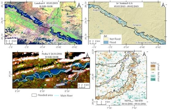
We tested the possibility of mapping the flooded areas of all our case studies manually. In some cases, this mapping was possible, mainly if a co-flood image was available. In general, areas covered by water are clearly visible on multispectral or SAR images, and the manual drawing can be done. In particular, false color images (Figure 4) made by using SWIR-NIR-BLUE bands of multispectral data allow better definition of the inundated areas. The main advantage of visual mapping is the possibility of minimizing errors (e.g., false positives and false negatives) of the semi-automatic classification methods, using geomorphological criteria during drawing. Conversely, the manual mapping is more time-consuming and requires the operator to possess experience in geomorphology and the dynamics of floods.
Figure 4 shows examples in our study areas of visual interpretation using remote sensing data.
- In the Ebro valley near Zaragoza (Figure 4A), we used a Landsat-8 co-flood image acquired on 2 March 2018; in this case, the false-color image allowed mapping the entire flooded area.
- In the Po River basin, around Alessandria town (Figure 4C), we used the Proba-V image acquired in the morning of 26 November 2016. In this case, it was possible to map most of the area flooded by Tanaro River, but the area flooded by Bormida River was not clearly detectable.
- In the Po River basin, at the South of Turin city (Figure 4B), the Sentinel-2 post-flood image shows only weak traces, and the semi-automatic classifications better identified the inundated area.
- In the Arahal area (Figure 4D), the Sentinel-2 post-flood image shows flood traces that are very difficult to detect, and the manual mapping fails. Here, we needed to use the automatic extraction of the flooded area for more reliable results.
In most of the considered cases, the polygon of flooded areas drowned manually needs refinement via DEM and other ancillary data.
4.2. Semi-Automatic Mapping of the Flooded Area
The applied semi-automatic approach consists of initially elaborating the co-flood images or the post- and pre-flood images. For each type of elaboration, we defined an empirical threshold that allowed detecting of the flooded area. All of this processing was done in QGIS software, and the automatic flood maps are in raster format.
4.2.1. SAR Data Analysis
In this section, we show the results of the SAR data-based analysis performed by using SAR amplitude classifications (SAR_AC) (Figure 5) and Δσo backscattering variation in Figure 6:
- SAR_AC. In the case of the Ebro River flood, the classification of the Sentinel-1 image acquired on 5 March 2015, i.e., two-three days after the flood peak (when most of the areas remain inundated according to MODIS data), allowed good detection of the flooded areas (Figure 5A). It is also possible to observe false positives, i.e., areas wrongly classified as flooded, most likely related to topographic artefacts or flat surfaces (e.g., airport ramp). Figure 5B shows the SAR_AC based on the Sentinel-1 image acquired on 28 November 2016 over the areas inundated by the Tanaro and Bormida Rivers near Alessandria. The flooded areas were detectable more easily for the Tanaro River, where the soil remained submerged two days after the flood peak, than for the Bormida River. The analysis performed over the area flooded by the Po River did not show significant results. In the Arahal area, the flooded area was partially detected with images acquired in the early morning of 29 November 2017, a few hours before the flood peak (Figure 5C).
- Δσo backscattering variation-based analysis. Compared with the SAR_AR-based analysis, such an approach allows achieving more-accurate results by exploiting calibrated Sentinel-1 data and image log ratios between the post- and pre-flood images (i.e., Δσo = log σo post-log σo pre). In addition, the comparison with pre-flood data allowed discriminating flooded areas from permanent water bodies. For most of the cases, we used VH polarization and Δσo > 0.6 as a threshold. In the case of Zaragoza (Figure 6A), we used the post-flood image of 5 March 2015 (acquired three days after the discharge peak), and the pre-flood image of 9 February 2015. The flooded area was partially detected with the semi-automatic methodology. However, this result allowed mapping of the entire inundated area with a visual interpretation. The results are also in agreement with MODIS data acquired on the same date. The comparison with a water-depth model showed that the areas remaining classified as flooded on the Sentinel-1 image approximately correspond to regions in which the water depth during the flood peak was higher than 1.5 m. In the case of Alessandria and Turin, we used the post-flood image of 28 November 2016 and the pre-flood image of 22 November 2016. Results show residual inundated areas. In particular, as already mentioned, the flooding pattern remains visible in the case of Tanaro River but not for the southern region of Turin, in which the remaining flooded areas are too small to be detected with Sentinel-1 data. In the case of Arahal (Figure 6D), we used VV polarization, which showed better performance concerning VH. We compared pre-flood (23 November 2017) with near co-flood images of 29 November 2017. In this case, we found that the threshold of 0.3 was the best value to detect flooded areas. The Sentinel-1 image was acquired in the early morning of 29 November 2017, some hours before the flood peak; most likely, the inundated areas are underestimated.
In all of our study areas, the capability to map flooded areas by SAR data is also limited by the presence of dense arboreal vegetation (small areas in the Ebro valley) or dense urban settlements (area of Moncalieri [57]). This limitation is already known in the literature [26]; more-complex SAR processing was developed to detect flooded areas in forested or urban areas [88,89]; moreover commercial L-Band satellites (e.g., ALOS-2) have better performance on forested areas [90].
4.2.2. Multispectral Data Analysis
In this section, we present the results of the multispectral analyses relying on single data methods (e.g., supervised classification) and on methods based on two-image comparisons.
(a) Supervised classification.Figure 7 shows the supervised classification based on MODIS and Landsat-8 multispectral images. We have defined four primary land-use typologies: Vegetation, urban area and bare soils, water body/wetland (that mostly correspond to the flooded areas) and cloud cover. The supervised classification showed good results for both the 2 March 2015 MODIS-Terra image (Figure 7A) and the 3 March 2015 Landsat-8 (Figure 7B) collected over the Ebro River valley, for which the scenes were almost cloud-free and the river was at the maximum discharge. The Landsat-8-based classification showed errors in the areas where the vegetation emerged from the water. The details were provided by the finest resolution. In the case of the Po basin flood, the supervised classification of the 26 November 2016 MODIS-aqua image (12–24 h after the flood peak) showed an underestimation of the flooded areas in the sectors inundated by the Bormida (Figure 7C) and by the Oitana and Chisola streams (Figure 7D). Classification errors due to partial cloud cover and shadow classified as water can be seen in the area around Alessandria (Figure 7C), but they do not significantly affect flood detection.
(b) Post-Pre flood image comparison. The comparison of co-flood or post-flood images with pre-flood images allowed mapping the flooded areas using different band-ratio variations.
(I) The MNDWIvar shows different performances depending upon the time of the satellite pass and local area setting. The threshold used to detect flooded areas ranged from 0.1 to 0.2. There was a decrease in the efficacy of this index with time elapsed from the flood event.
In the Zaragoza case study (Figure 8A), the flooded area was almost entirely detected by the co-flood Landsat-8 image acquired on 3 March 2015. Some false positive variation at SW is related to cloud cover. The MNDWIvar computed with the 2 March 2015 MODIS image provided the same results.
In the case of the November 2016 Po basin flood, only post-flood data are available at high resolution. At south of Turin, the flooded areas were satisfactorily detected with the 26 November 100 m spatial resolution Proba-V image (Figure 8B), whereas by using Sentinel-2 imagery acquired (Figure 8C) five days after the water was withdrawn, it remains possible to detect a pattern of positive MNDWIvar inside the inundated areas, but with more false positive areas. Over the Alessandria area, the MNDWI based on 100 m spatial resolution Proba-V (Figure 8E) and 500 m spatial resolution Proba-V (Figure 8E) data acquired approximately 8–12 h after the flood peak detected most of the areas inundated by Tanaro, despite cloud cover and shadows. Sentinel-2 images (Figure 8F) acquired approximately 10 days after the flood peak only show residual patterns. Many pixels located out of flooded areas are classified as inundated, most likely due to a general increase of soil moisture. We also applied a cloud mask to the images of 26 November of MODIS and Proba-V; fortuitously, the cloud cover and shadow did not affect the detection of the flooded area.
In the case of the Arahal flood (Figure 8F), the MNDWIvar based on the Sentinel-2 image acquired 10 days after the flood event allowed the detection of only some residual parts of the original flood. The NDMIvar based on Landsat images showed a similar result.
(II) In the case of the 2016 Po basin flood (Figure 9), we also calculated the NDVIvar and the VISvar to extract the flooded area automatically. The areas affected by floods show a negative variation of NDVI most likely related to a decrease of vegetation activity due to the deposition of silt layers or damages (e.g., broken stems of the crop). This effect is particularly evident in the wheat fields outside the flooded areas, showing an increase of NDVI. Moreover, for the NDVIvar method, the capability to detect flooded areas decreases with the time elapsed from the flood peak. This decreasing trend is independent of the spatial resolution of the satellite. The NDVIvar made by using the MODIS-Aqua images collected on 30 November 2016 and 12 November 2016 at a spatial resolution of 250 m/pixel shows a clear pattern of the flooded area for both the Po (Figure 9E) and Tanaro areas (Figure 9D).
Moreover, the high-resolution NDVIvar based on Sentinel-2 data continues to shows a pattern of negative variation both in the South Turin area with an image acquired on 1 December (Figure 9B) and in the Alessandria area with the 8 December images (Figure 9A,C). The VISvar shows a clear pattern of positive variation only for the area flooded by the Tanaro River nearby Alessandria (Figure 9B) due to the widespread deposition of silt sediments covering the area two weeks after the inundation. The areas flooded by the Po and other rivers showed less evidence of sediment; accordingly, the VISvar analysis is less performant.
4.3. Flood, Mapping Refinement Using Water Depth DEM and Ancillary Data
As already mentioned, the second step for the flood map creation is the refinement and improvement based on supporting data (i.e., DEM and ancillary data), the result of which is particularly useful when we have flood maps based only on post-flood images. The final result was the production of flooded area manually drawn polygons. Figure 10 shows an example of the integration of remote sensing data, DEM modelling and ancillary data for the mapping of the areas flooded by the Tanaro River near Alessandria. The map in Figure 10A represents the inundation area derived from the semi-automatic classification of remote sensing images based, in this case, on VISvar of Sentinel-2 data.
Figure 10B shows the inundation maps based on a water depth (WD) model in which the pixel is classified as inundated when WD > 0 m,
Figure 10C represents the synthesis of the two presented maps, in which a pixel is classified as inundated if flooded in both satellite data and the WD model. The WD model allowed reducing pixels incorrectly classified as flooded (false positive). Furthermore, the geolocated photos (available on websites or from volunteers) allowed us to have some ground truth points.
Figure 10D represents the final version of the flooded area that was manually drawn considering the remote sensing data, the WD model, and the ancillary data.
We also used the same methods to create the final maps of the area flooded by the Po and Ebro Rivers. The refinement step was handy for the case of the Po River, whereas for the Ebro, for which the high-resolution co-flood map is available, the support data do not provide significant improvement.
For the Arahal case study, in which the flooded area was more difficult to detect, we made a more in-depth effort to combine satellite and support data. Figure 11 shows the steps used to create the refined flood map.
We initially created a semi-automatic map of the flooded area (Figure 11A) by crossing all of the available remote sensing data (i.e., Landsat-8, Sentinel-2 and Sentinel-1). Then, we created a WD model map for the two small streams affected by the flood, around the intersection with the Seville-Malaga railway (Figure 11B). The combination of such a model with remote sensing data allowed us to produce the map of the estimated flooded area (Figure 11C). To assess the reliability of the flood map, we exploited geolocated photos and news about the flood. Available images allowed an evaluation of the reliability of the inundation map locally, e.g., it was possible to locate the effect of embankment erosion on a railway line (photo 3).
4.4. Flood Map Validation and Statistics
The last step of the presented methodology consists of validating the automatic flood maps. We applied the validation to the flood maps of Ebro valley and the Po basin using the official flood maps of the Ebro River authority (CHE) and ARPA Piemonte.
The validation process, as described earlier, is based on the definition of a raster validation map. In these raster maps, each pixel can assume four values: (0) True negative (TN) case represented in brown; (1) false positive (FP) case represented in cyan; (2) false negative (FN) case represented in yellow; and (3) true positive (TP) case represented in blue. To make a more homogeneous comparison, the area covered by a permanent water body was not calculated in FR or NFR.
In Figure 12, examples of validation maps for semi-automatic flooded area maps are reported. For the area of Zaragoza (Figure 12A), the MNDWIvar derived from co-flood Landsat-8 images allowed correctly classifying both flooded and not-flooded areas (>90%); the Δσo Sentinel-1-based analysis (Figure 13B) also shows satisfactory performance (FR 50%; NFR > 90%).
For the area of Alessandria, the NDVIvar computed from the MODIS-Terra data shows better results (FR 70%, Figure 12C) compared with the Δσo-based analysis (FR of 30%, Figure 12D).
In the area at the south of Turin, the MNDWIvar (Figure 13E) made with a post-flood image (1 December 2016) from Sentinel-2 data detected approximately 45% of the flooded area.
We also applied the validation to the final refined maps of flooded areas. The results show that our maps mostly coincide (FR > 90%) with official maps of ARPA Piemonte and the Ebro River authority in the case of Zaragoza and Alessandria, but more differences can be found in the maps flooded by the Po (FR 70%).
Figure 13 shows a correlation between the river levels for the Ebro (Figure 13A), Tanaro (Figure 13B) and Po (Figure 13C) with the flood ratio (FR) for semi-automatic flood mapping based on different methodologies and satellites. The results give an idea of the various parameters that influence flooded area detection. In general, the quality of semi-automatic detection of flooded areas decreases with the time after the peak of the flood for all of the cases considered. The SAR data show a much more rapid decrease in the capacity to detect flooded areas.
For each area, the primary results are as follows:
- The area flooded by the Ebro River near Zaragoza in 2015 (Figure 13A). In this case, co-flood data at low resolution (MODIS-Terra/Aqua and Proba-V) and medium-high resolution (Landsat-8) allowed mapping the entire flooded area (FR > 95%) with few false positive values. In this case, spatial resolution has little influence on the accuracy of flooded area detection. The Δσo map made with Sentinel-1 data acquired two days after the maximum flood shows that approximately 50% of the area is detectable with an NFR (≈98%). With the map based on Sentinel-1 data, it was nonetheless possible to detect a clear pattern that identifies entire flooded areas.
- The area flooded by Tanaro near Alessandria in 2016 (Figure 13B). Here, there are high values of FR for near co-flood data of MNDWI based on MODIS-Aqua (FR ≈ 90%) and Proba-V (FR ≈ 82%). For a post-flood image, the relationship “time of flood peak vs. time of satellite pass” is more important than spatial resolution; 250 m NDVI based on MODIS data of 30 November 2016 show a better result (FR ≈ 80%) than do 10 m NDVI based on Sentinel-2 of 8 December 2016 (FR ≈ 60%). SAR data based on 28 November imagery from Sentinel-1 show low values of FR (≈20%), making detecting the entire flooded area more complicated. Another critical factor influencing flood detection with post-flood data is the local conditions. In particular, the presence of a thin layer of silt deposits on crop fields helped the identification of the inundated area. Two weeks after the flood, the VISvar based on Sentinel-2 data showed an FR of 70% and NFR ≈ 84%
- The area flooded by the Po at the south of Turin, compared with Carignano gauge (Figure 13C). Here, the flood detection presented results similar to those of the Alessandria area. In particular, Sentinel-2 data acquired on 1 December 2016 show better results for MNDWIvar (≈50% FR) with respect to NDVIvar. (≈35% FR). It was not possible to the map the flooded area with Δσo of Sentinel-1 because three days after the flood peak, only 4% of the inundated area was detected. For this area, the accuracy in flood detection is also unrelated to spatial resolution; the best performance comes from MNDWI based on the MODIS image of 26 November 2016 (FR ≈ 80%).
4.5. Comparing Flood-Mapping Approaches: Automatic Emergency, Traditional and Combined Approach
For the case of the 2015 Ebro and 2016 NW Italy floods, Figure 14 shows a comparison between the flooded areas mapped by EMS-Copernicus [52,58], the flooded area made with manual interpretation for this work and the official flood maps produced by river authorities.
The EMS-Copernicus mapping is automatic mapping in quasi-real time that identifies critical areas during the emergency but does not represent the real flood extent for further post-emergency analyses. For instance, the EMS flood mapping in the case of the Alessandria area (Figure 14A) is based on Radarsat-2 data (acquired on 27 November 2016), and the map shows only the remaining flooded areas (dark blue). The EMS underestimates the flooded area with respect to the results of this work and official maps.
The area at the south of Turin (Figure 14B) was partially mapped by EMS only from Carignano downstream to Turin. The flood map for the area near Moncalieri, investigated with Pleiades satellite at 26 November 2016, detected most of the flooded areas and fitted well with our map. The sector near Carignano town, mapped with an image of 27 November 2016, shows only residual flooded areas.
In the case of Ebro valley, the EMS flood map was made with a Radarsat-2 image acquired on 2 March 2015 (Figure 14C). The map shows an almost complete fit with our flood mapping and the official flood mapping of CHE.
The comparison with official mapping showed good results. The flood maps made for this study based on remote sensing data match well with the official maps of the Ebro basin authority (CHE) with a 95% overlap (Figure 14C). The area inundated by Tanaro (Figure 14A) proposed in this study also shows a good match, approximately 90%, with ARPA Piemonte flood maps. There are more differences in the area at the south of Turin (approximately 85% matching, Figure 14B); this sector is mapped mostly with post-flood data, and the areas affected by shallow water depth have fewer signs of the flood. Flood mapping based on satellite data presented more challenge in the urban areas, in which a more detailed survey is often required, as shown in a previous work [47].
In the case of the Arahal flood, it is not possible to estimate the accuracy of flood mapping because official maps are not available. However, the combination of Sentinel-1, Landsat-8, and Sentinel-2 data implemented with a water depth model allowed creating a reliable map that was locally validated.
5. Discussion
The results of our study show that choosing the best satellite data or the most appropriate processing aimed at detecting flooded areas is a complicated process. It is necessary to consider the complex relationships between the flood and the satellite characteristics. In the following, we introduce a more detailed description of the parameters that play a fundamental role:
- The time factor is the most critical parameter. If a co-flood image is available, the detection and the refinement of the inundated area are more straightforward and require a short time. To know the time of maximum inundation, data from river gauge stations (e.g., for the Ebro, Po, and Tanaro case studies) can be considered. If river gauge station data are not available (e.g., Arahal case study), it is often possible to estimate the time of inundation from ancillary data found on the web such as news, photos, or videos. Medium-low resolution multispectral satellites (MODIS, Proba-V, Sentinel-3), with their daily revisit time, are more likely to acquire co-flood images for many flood events. However, it is less probable to have co-flood SAR images acquired by Sentinel-1, which in 2018 are the only SAR satellites providing free images. The time elapsed from the flood peak also influences the band ratios to use; MNDWIvar shows better performance in the short term, whereas NDVIvar and VISvar have better performances over the long term because MNDWI is more sensitive to open water; changes in NDVI and VIS are primarily related to vegetation damage or silt deposits in flooded areas. Concerning the pre-flood images used as a benchmark, the one acquired as close as possible to the flood event should be selected to have similar conditions of land use and sun illumination.
- The use of a single acquisition date with respect to image differences with pre-flood must be considered in the semi-automatic mapping: In the first case, permanent water bodies outside flooded areas are wrongly classified as flooded. In the second case, the water bodies inside the flooded area are not classified as flooded. This issue can be solved using a mask of the permanent water body.
- The sky-condition is another relevant parameter that limits the availability of co-flood images. Indeed, only SAR satellites can acquire images under cloudy conditions. In our cases, the area flooded around Zaragoza was cloud free during the 2015 flooding because the flood peak arrived several days after the meteorological event, whereas cloudy conditions did limit the availability of images for the 2016 Po basin flood.
- The spatial features of the flooded area represent a constraint on satellite spatial resolution. Small, inundated areas (e.g., Arahal case study) cannot be mapped by low-resolution satellites. In addition, an area flooded by a small stream has a very short co-flood time interval.
- The extent of the affected area. For the main river, it might require more than one image to map the whole river section affected by the flood. In addition, the time of maximum flood changes along the stream and is not the same for tributaries. For instance, the flood waves of the Po and Ebro Rivers transited over several days from upstream to downstream.
- Land use and morphology of the flooded area. These factors are important in choosing the satellite image. Inundations occurring on cultivated crops in floodplains can be easily detected by most satellites. In addition, several days after the flood, with multi-spectral data, it is possible to recognize flooded areas easily, particularly if sediments cover crop fields. In urban or densely forested regions, detection of the flooded areas is more complicated. In the arid region, the effect on NDVI can be opposite, with an increase of vegetation index in the flooded area [67]. In many cases, high-resolution data and field surveys remain necessary for a reliable mapping.
- With the semi-automatic approach, we used empirical thresholds to detect flooded areas. The semi-automatic approach allows selecting the best threshold that defines a geomorphological based pattern of the flooded area. Conversely, the semi-automatic approach requires specific operator experience in flood dynamics.
- Results also show that the direct visual mapping of flooding areas can be performed only when the flooded area is visible in co-flood images. Otherwise, it is better to use semi-automatic detection followed by the refinement step.
In the presented study, we used only cost-free satellite data that allowed us to create reliable flood maps. One of the most important features of the used satellite data is their continuous temporal sampling and the rapid revisiting time. For example, MODIS satellites provide multispectral images on a daily basis, which allows having free cloud images close to the flood peak for the Ebro and Po flood areas. The Sentinel-1 system continually provides SAR data with short revisit times and global coverage, and Sentinel-2 satellites allowed the creation of flood maps with very good spatial resolution.
However, if we must map floods affecting dense urban areas with high accuracy or produce an exact flood water depth map for damage assessment, we must exploit high-resolution (satellite, aerial or terrestrial) data. Very often, the required high-resolution data are not free, for example, the 2016 Chisola stream, which flooded the Moncalieri town, as described in previous work [57].
In this work, we also exploited free ancillary data such as DEM, river gauge data, and geolocated information. Our areas of study were covered by free and high-resolution DEMs provided by local authorities and, for the Ebro and Po basins, were covered by gauge station networks providing river level data with a good density. As described earlier, these ancillary datasets are fundamental for a better definition of the limits of the flooded area.
6. Conclusions
In this study, we presented a methodology for low-cost and user-friendly flood mapping based on free satellite data jointly exploited with free ancillary data. In particular, we used data from Sentinel-1, Sentinel-2, Landsat-8, Proba-V and MODIS Terra/Aqua satellites and processed them with open-source software based-methods easily carrying out also by non-remote sensing expert community. We tested our methodology over three areas recently hit by floods: (i) The Ebro valley near Zaragoza, Spain, flooded in spring 2015; (ii) two areas near Alessandria and Turin (Piemonte region, NW Italy) inundated by Po, Tanaro, and their tributaries in November 2016; and (iii) a small area around the Arahal village, southern Spain, affected by a flash flood in November 2017.
The proposed flood mapping strategy is composed of progressive steps. Firstly, the detection of flooded area is performed, through semi-automatic extraction or by visual interpretation of satellite images. The flood map is later manually refined with the help of ancillary data such as digital elevation models (DEMs), water depth (WD) models or ground photos and web-based information. The final outcome is an accurate and morphologically based flood map in vector format.
In the presented case studies, we validate the methodology results with available flooded area maps provided by local authorities. For the case of the Ebro and Po basin flood, we considered a performance assessment of the different automatic maps, and we calculated the flood ratio (FR), which is the percentage of the flooded area detected by satellites with respect to official maps.
The study points out that the capability of spaceborne sensors to map a flood event depends upon several factors: (a) The time of the satellite pass with respect to the time of the flood peak, that is the most important factor; (b) the spatial resolution of satellite; (c) the sensors type (e.g., SAR or multispectral); (d) the sky conditions; (e) the land-use and morphology of the flooded area; (f) the type of data processing.
The results show that SAR-based flood mapping is more efficient when co-flood acquisitions are available, allowing the extraction of information on areas fully covered by water also in cloudy or night conditions. However, the only SAR system currently providing free and open data is Sentinel-1; for this reason, the availability of co-flood data is limited. In our study, a co-flood Sentinel-1 image was available only for the 2015 Ebro valley flood, allowing a satisfactory detection of the flooded area (≈50% FR). In the other study areas, only post-flood SAR data were available; these data, although acquired a few hours or days after the water withdrawal, were not suitable for flood mapping: FR showed values of about 20% for the area flooded by Tanaro to less than 5% for the area inundated by the Po River.
In the case of multispectral data-based mapping instead, the analysis shows that post-flood acquisitions can be profitably exploited, allowing to detect changes inside the flooded areas within a few weeks after water withdrawal. The results show that the FR decreases with the time elapsed from the flood peak but slower respect to SAR: For instance, the computed MNDWIvar decreases from values >90% with co-flood imagery to less than 50% if the available imagery is acquired two weeks later in all the flooded areas. It is worth noting that the local conditions, such as the depositions of silt sediments, contribute to mapping the flooded areas for a more extended period: e.g., VISvar showed a FR≈ 70% in the area flooded by the Tanaro using Sentinel-2 data acquired 15 days after the floods.
The MODIS and Proba-V satellite sensors, with a daily revisit time, increase the probability of acquiring co-flood data and allow achievement of very good results despite the medium-low spatial resolution. In the Zaragoza area, the MODIS and Proba-V co-flood images allowed a very accurate mapping (FR >90%). For the area of Alessandria, quasi co-flood Proba-V data permitted achieving excellent results, with a FR of nearly 100% for the area flooded by the Tanaro.
The analysis that relied on medium-high resolution Landsat-8 and Sentinel-2 data shows the same flood ratio performance as the medium-low resolution satellites (FR > 90% for co-flood Landsat images in Zaragoza areas) but with a spatial precision several times greater. These data indeed also allowed the detection of small, flooded areas (up to ≈500 m2). In particular, the high-resolution was very useful for the Arahal flash-flood case study. In this case, the availability and the combination of high-resolution Sentinel-2, Sentinel-1 and Landsat-8 data joined with ancillary data and geomorphological interpretation was fundamental to producing a reliable flood map.
The study points out some drawbacks of flood mapping based on the use of SAR and multispectral satellite data. In the latter case, the main limitation is represented by cloud cover affecting co-flood multispectral acquisitions. The presence of clouds has indeed limited the flooded areas detection in the case of the Po flood, while has not affected the Ebro study because the inundation occurred several days after the rainfall event.
The presence of dense urban areas and forests affects both SAR and multispectral based flood mapping and requires a more-complex data processing which is not straightforward to accomplish with a user-friendly approach. High spatial resolution is also a key factor when mapping floods in dense urban areas, and it is one of the limitations of the free of charge satellite data approach. Based on our experience, on-demand high costs, high resolution data and field surveys are often necessary [57].
However, despite such drawbacks the integration of freely available satellite data with ancillary data allowed us to map about 450 km2 of inundated areas with high accuracy for all studied areas.
Our methodology proves to be a good trade-off between emergency real-time automatic flood mapping and the traditional flood mapping performed with on-demand data. Real-time automatic flood mapping (e.g., Copernicus EMS) are usually fast, but not very accurate. In contrast, traditional flood mapping performed with on-demand data provides very accurate results, but it is a more resource-intensive process.
Furthermore, we propose a user-friendly approach for satellite data processing that can also be exploited by users with no remote sensing expertise, contributing to hydrological studies, urban planning or flood hazard/damage assessment. In such a context, having a network of operational satellites providing free- and open-access data with continuity is of great importance for flood mapping and hazard/risk management in floodplain areas and disadvantaged regions worldwide.
Supplementary Materials
The following are available online at https://0-www-mdpi-com.brum.beds.ac.uk/2072-4292/10/11/1673/s1.
Author Contributions
D.N. is primarily responsible for the study, developing the work methodology, processing multispectral data and writing the manuscript. D.G. contributed to the writing and revision of the manuscript and coordinated the research project. F.C. and A.P. processed the Sentinel-1 data, wrote the InSAR processing chapter and revised the manuscript. F.Z. and J.P.G. contributed implementation and correction of the manuscript.
Funding
This research received no external funding.
Acknowledgments
The authors wish to acknowledge the volunteers that provided ground photos of the 2016 flood. We thank the three anonymous referees that revised the paper.
Conflicts of Interest
The authors declare no conflict of interest.
References
- Klein, T.; Nilsson, M.; Persson, A.; Håkansson, B. From Open Data to Open Analyses—New Opportunities for Environmental Applications? Environments 2017, 4, 32. [Google Scholar] [CrossRef]
- Turner, W.; Rondinini, C.; Pettorelli, N.; Mora, B.; Leidner, A.K.; Szantoi, Z.; Buchanan, G.; Dech, S.; Dwyer, J.; Herold, M. Free and open-access satellite data are key to biodiversity conservation. Biol. Conserv. 2015, 182, 173–176. [Google Scholar] [CrossRef] [Green Version]
- Li, S.; Dragicevic, S.; Castro, F.A.; Sester, M.; Winter, S.; Coltekin, A.; Pettit, C.; Jiang, B.; Haworth, J.; Stein, A. Geospatial big data handling theory and methods: A review and research challenges. ISPRS J. Photogramm. Remote Sens. 2016, 115, 119–133. [Google Scholar] [CrossRef] [Green Version]
- Wulder, M.A.; Masek, J.G.; Cohen, W.B.; Loveland, T.R.; Woodcock, C.E. Opening the archive: How free data has enabled the science and monitoring promise of Landsat. Remote Sens. Environ. 2012, 122, 2–10. [Google Scholar] [CrossRef]
- Berger, M.; Moreno, J.; Johannessen, J.A.; Levelt, P.F.; Hanssen, R.F. ESA’s sentinel missions in support of Earth system science. Remote Sens. Environ. 2012, 120, 84–90. [Google Scholar] [CrossRef]
- Hansen, M.C.; Loveland, T.R. A review of large area monitoring of land cover change using Landsat data. Remote Sens. Environ. 2012, 122, 66–74. [Google Scholar] [CrossRef]
- Justice, C.O.; Vermote, E.; Townshend, J.R.; Defries, R.; Roy, D.P.; Hall, D.K.; Salomonson, V.V.; Privette, J.L.; Riggs, G.; Strahler, A. The Moderate Resolution Imaging Spectroradiometer (MODIS): Land remote sensing for global change research. IEEE Trans. Geosci. Remote Sens. 1998, 36, 1228–1249. [Google Scholar] [CrossRef]
- EOSDIS Worldview. Available online: https://worldview.earthdata.nasa.gov/ (accessed on 6 March 2018).
- Cignetti, M.; Manconi, A.; Manunta, M.; Giordan, D.; De Luca, C.; Allasia, P.; Ardizzone, F. Taking advantage of the ESA G-pod service to study ground deformation processes in high mountain areas: A valle d’aosta case study, northern Italy. Remote Sens. 2016, 8, 852. [Google Scholar] [CrossRef]
- Galve, J.P.; Pérez-Peña, J.V.; Azañón, J.M.; Closson, D.; Caló, F.; Reyes-Carmona, C.; Jabaloy, A.; Ruano, P.; Mateos, R.M.; Notti, D. Evaluation of the SBAS InSAR Service of the European Space Agency’s Geohazard Exploitation Platform (GEP). Remote Sens. 2017, 9, 1291. [Google Scholar] [CrossRef]
- Congedo, L. Semi-automatic classification plugin documentation. Release 2016, 4, 29. [Google Scholar]
- Ward, P.J.; Jongman, B.; Weiland, F.S.; Bouwman, A.; van Beek, R.; Bierkens, M.F.; Ligtvoet, W.; Winsemius, H.C. Assessing flood risk at the global scale: Model setup, results, and sensitivity. Environ. Res. Lett. 2013, 8, 044019. [Google Scholar] [CrossRef] [Green Version]
- Moel, H.D.; Alphen, J.V.; Aerts, J. Flood maps in Europe–methods, availability and use. Nat. Hazards Earth Syst. Sci. 2009, 9, 289–301. [Google Scholar] [CrossRef] [Green Version]
- Amadio, M.; Mysiak, J.; Carrera, L.; Koks, E. Improving flood damage assessment models in Italy. Nat. Hazards 2016, 82, 2075–2088. [Google Scholar] [CrossRef] [Green Version]
- Ran, J.; Nedovic-Budic, Z. Integrating spatial planning and flood risk management: A new conceptual framework for the spatially integrated policy infrastructure. Comput. Environ. Urban Syst. 2016, 57, 68–79. [Google Scholar] [CrossRef]
- Fayne, J.; Bolten, J.; Lakshmi, V.; Ahamed, A. Optical and Physical Methods for Mapping Flooding with Satellite Imagery. In Remote Sensing of Hydrological Extremes; Springer: Berlin/Heidelberg, Germany, 2017; pp. 83–103. [Google Scholar]
- Musa, Z.N.; Popescu, I.; Mynett, A. A review of applications of satellite SAR, optical, altimetry and DEM data for surface water modelling, mapping and parameter estimation. Hydrol. Earth Syst. Sci. 2015, 19, 3755–3769. [Google Scholar] [CrossRef] [Green Version]
- Schumann, G.; Bates, P.D.; Apel, H.; Aronica, G.T. Global Flood Hazard Mapping, Modeling, and Forecasting: Challenges and Perspectives. Glob. Flood Hazard Appl. Model. Mapp. Forecast. 2018, 239–244. Available online: https://0-agupubs-onlinelibrary-wiley-com.brum.beds.ac.uk/doi/10.1002/9781119217886.ch14 (accessed on 20 October 2018).
- Chen, Y.; Huang, C.; Ticehurst, C.; Merrin, L.; Thew, P. An evaluation of MODIS daily and 8-day composite products for floodplain and wetland inundation mapping. Wetlands 2013, 33, 823–835. [Google Scholar] [CrossRef]
- Nigro, J.; Slayback, D.; Policelli, F.; Brakenridge, G.R. NASA/DFO MODIS Near Real-Time (NRT) Global Flood Mapping Product Evaluation of Flood and Permanent Water Detection. Eval. Greenbelt MD 2014. Available online: https://floodmap.modaps.eosdis.nasa.gov/documents/NASAGlobalNRTEvaluationSummary_v4.pdf (accessed on 20 October 2018).
- Wang, Y.; Colby, J.D.; Mulcahy, K.A. An efficient method for mapping flood extent in a coastal floodplain using Landsat TM and DEM data. Int. J. Remote Sens. 2002, 23, 3681–3696. [Google Scholar] [CrossRef]
- Rahman, M.S.; Di, L. The state of the art of spaceborne remote sensing in flood management. Nat. Hazards 2017, 85, 1223–1248. [Google Scholar] [CrossRef]
- Ticehurst, C.; Guerschman, J.P.; Chen, Y. The strengths and limitations in using the daily MODIS open water likelihood algorithm for identifying flood events. Remote Sens. 2014, 6, 11791–11809. [Google Scholar] [CrossRef]
- Chignell, S.M.; Anderson, R.S.; Evangelista, P.H.; Laituri, M.J.; Merritt, D.M. Multi-temporal independent component analysis and Landsat 8 for delineating maximum extent of the 2013 Colorado front range flood. Remote Sens. 2015, 7, 9822–9843. [Google Scholar] [CrossRef]
- Boni, G.; Ferraris, L.; Pulvirenti, L.; Squicciarino, G.; Pierdicca, N.; Candela, L.; Pisani, A.R.; Zoffoli, S.; Onori, R.; Proietti, C. A prototype system for flood monitoring based on flood forecast combined with COSMO-SkyMed and Sentinel-1 data. IEEE J. Sel. Top. Appl. Earth Obs. Remote Sens. 2016, 9, 2794–2805. [Google Scholar] [CrossRef]
- Schumann, G.J.-P.; Moller, D.K. Microwave remote sensing of flood inundation. Phys. Chem. Earth Parts ABC 2015, 83, 84–95. [Google Scholar] [CrossRef]
- Refice, A.; Capolongo, D.; Pasquariello, G.; D’Addabbo, A.; Bovenga, F.; Nutricato, R.; Lovergine, F.P.; Pietranera, L. SAR and InSAR for flood monitoring: Examples with COSMO-SkyMed data. IEEE J. Sel. Top. Appl. Earth Obs. Remote Sens. 2014, 7, 2711–2722. [Google Scholar] [CrossRef]
- Pulvirenti, L.; Chini, M.; Pierdicca, N.; Guerriero, L.; Ferrazzoli, P. Flood monitoring using multi-temporal COSMO-SkyMed data: Image segmentation and signature interpretation. Remote Sens. Environ. 2011, 115, 990–1002. [Google Scholar] [CrossRef]
- Clement, M.A.; Kilsby, C.G.; Moore, P. Multi-temporal synthetic aperture radar flood mapping using change detection. J. Flood Risk Manag. 2017. [Google Scholar] [CrossRef]
- Twele, A.; Cao, W.; Plank, S.; Martinis, S. Sentinel-1-based flood mapping: A fully automated processing chain. Int. J. Remote Sens. 2016, 37, 2990–3004. [Google Scholar] [CrossRef]
- Cian, F.; Marconcini, M.; Ceccato, P. Normalized Difference Flood Index for rapid flood mapping: Taking advantage of EO big data. Remote Sens. Environ. 2018, 209, 712–730. [Google Scholar] [CrossRef]
- D’Addabbo, A.; Refice, A.; Pasquariello, G.; Lovergine, F. SAR/optical data fusion for flood detection. In Proceedings of the IEEE International on Geoscience and Remote Sensing Symposium (IGARSS), Beijing, China, 10–15 July 2016; pp. 7631–7634. [Google Scholar]
- Demirkesen, A.C.; Evrendilek, F.; Berberoglu, S.; Kilic, S. Coastal flood risk analysis using Landsat-7 ETM+ imagery and SRTM DEM: A case study of Izmir, Turkey. Environ. Monit. Assess. 2007, 131, 293–300. [Google Scholar] [CrossRef] [PubMed]
- Gianinetto, M.; Villa, P.; Lechi, G. Postflood damage evaluation using Landsat TM and ETM+ data integrated with DEM. IEEE Trans. Geosci. Remote Sens. 2006, 44, 236–243. [Google Scholar] [CrossRef]
- Pierdicca, N.; Chini, M.; Pulvirenti, L.; Macina, F. Integrating physical and topographic information into a fuzzy scheme to map flooded area by SAR. Sensors 2008, 8, 4151–4164. [Google Scholar] [CrossRef] [PubMed] [Green Version]
- Brivio, P.A.; Colombo, R.; Maggi, M.; Tomasoni, R. Integration of remote sensing data and GIS for accurate mapping of flooded areas. Int. J. Remote Sens. 2002, 23, 429–441. [Google Scholar] [CrossRef]
- Chen, J.L.; Wilson, C.R.; Tapley, B.D. The 2009 exceptional Amazon flood and interannual terrestrial water storage change observed by GRACE. Water Resour. Res. 2010, 46. [Google Scholar] [CrossRef] [Green Version]
- Massari, C.; Camici, S.; Ciabatta, L.; Brocca, L. Exploiting Satellite-Based Surface Soil Moisture for Flood Forecasting in the Mediterranean Area: State Update Versus Rainfall Correction. Remote Sens. 2018, 10, 292. [Google Scholar] [CrossRef]
- Malinowski, R.; Groom, G.B.; Heckrath, G.; Schwanghart, W. Do Remote Sensing Mapping Practices Adequately Address Localized Flooding? A Critical Overview. Springer Sci. Rev. 2017, 5, 1–17. [Google Scholar] [CrossRef]
- Copernicus Emergency Management Service. Available online: http://emergency.copernicus.eu/mapping/list-of-components/EMSR120 (accessed on 7 March 2018).
- Ajmar, A.; Boccardo, P.; Broglia, M.; Kucera, J.; Wania, A. Response to flood events: The role of satellite-based emergency mapping and the experience of the Copernicus emergency management service. Flood Damage Surv. Assess. New Insights Res. Pract. 2017, 213–228. [Google Scholar] [CrossRef]
- Kugler, Z.; De Groeve, T. The global flood detection system. In JRC Scientific and Technical Reports; JRC: Ispra, Italy, 2007; pp. 1–45. Available online: http://publications.jrc.ec.europa.eu/repository/handle/JRC44149 (accessed on 20 October 2018).
- Global Floods Detection System. Available online: http://www.gdacs.org/flooddetection/overview.aspx (accessed on 7 March 2018).
- Policelli, F.; Slayback, D.; Brakenridge, B.; Nigro, J.; Hubbard, A.; Zaitchik, B.; Carroll, M.; Jung, H. The NASA global flood mapping system. In Remote Sensing of Hydrological Extremes; Springer: Berlin/Heidelberg, Germany, 2017; pp. 47–63. [Google Scholar]
- Revilla-Romero, B.; Hirpa, F.A.; Pozo, J.T.; Salamon, P.; Brakenridge, R.; Pappenberger, F.; De Groeve, T. On the use of global flood forecasts and satellite-derived inundation maps for flood monitoring in data-sparse regions. Remote Sens. 2015, 7, 15702–15728. [Google Scholar] [CrossRef] [Green Version]
- Bales, J.D.; Wagner, C.R. Sources of uncertainty in flood inundation maps. J. Flood Risk Manag. 2009, 2, 139–147. [Google Scholar] [CrossRef]
- Balasch, J.C.; Pino, D.; Ruiz-Bellet, J.L.; Tuset, J.; Barriendos, M.; Castelltort, X.; Peña, J.C. The extreme floods in the Ebro River basin since 1600 CE. Sci. Total Environ. 2019, 646, 645–660. [Google Scholar] [CrossRef] [PubMed]
- Confederación Hidrográfica del Ebro (CHE). Informe Sobre las Avenidas del Primer Trimestre de 2015 en la Cuenca del Ebro; CHE: Zaragoza, Spain, 2015; Available online: ftp://ftp.chebro.es/memorias/Memoria2015.pdf (accessed on 20 October 2018).
- Anchuela, Ó.P.; Revuelto, C.; Sainz, A.C.; Cordero, J.R.; Pocoví, A. Las crecidas del Ebro de febrero/marzo de 2015.¿ Qué hemos aprendido y qué falta por aprender? Geogaceta 2016, 60, 119–122. [Google Scholar]
- Floods in Northern Spain as Ebro River Breaks its Banks–FloodList. Available online: http://floodlist.com/europe/floods-northern-spain-ebro-river (accessed on 7 March 2018).
- Foudi, S.; Osés-Eraso, N.; Tamayo, I. Integrated spatial flood risk assessment: The case of Zaragoza. Land Use Policy 2015, 42, 278–292. [Google Scholar] [CrossRef]
- Copernicus Emergency Management Service (© 2015 European Union), EMSR120-Floods in Spain. Available online: http://emergency.copernicus.eu/mapping/list-of-components/EMSR120 (accessed on 6 March 2018).
- Ebro River Authorithy (CHE) Geoportal. Available online: http://iber.chebro.es/geoportal/ (accessed on 7 March 2018).
- Luino, F. The flood and landslide event of 4–6 November 1994 in Piedmont Region (Northwestern Italy): Causes and related effects in Tanaro Valley. Phys. Chem. Earth Part Solid Earth Geod. 1999, 24, 123–129. [Google Scholar] [CrossRef]
- Pinto, J.G.; Ulbrich, S.; Parodi, A.; Rudari, R.; Boni, G.; Ulbrich, U. Identification and ranking of extraordinary rainfall events over Northwest Italy: The role of Atlantic moisture. J. Geophys. Res. Atmosp. 2013, 118, 2085–2097. [Google Scholar] [CrossRef] [Green Version]
- ARPA Piemonte. Evento Alluvionale 21–26 Novembre 2016. 2016. Available online: https://www.arpa.piemonte.it/pubblicazioni-2/relazioni-tecniche/analisi-eventi/eventi-2016/rapporto-preliminare-novembre-2016-def.pdf (accessed on 20 October 2018).
- Giordan, D.; Notti, D.; Villa, A.; Zucca, F.; Calò, F.; Pepe, A.; Dutto, F.; Pari, P.; Baldo, M.; Allasia, P. Low cost, multiscale and multi-sensor application for flooded area mapping. Nat. Hazards Earth Syst. Sci. 2018, 18, 1493–1516. [Google Scholar] [CrossRef]
- Copernicus Emergency Management Service (© 2016 European Union), EMSR192-Floods in Northern Italy. Available online: http://emergency.copernicus.eu/mapping/list-of-components/EMSR192 (accessed on 6 March 2018).
- Spain–Heavy Rain Floods Parts of Andalusia–FloodList. Available online: http://floodlist.com/europe/spain-floods-andalusia-november-2017 (accessed on 7 March 2018).
- Po River Agency (AIPO) Po River Stage at Carignano Gauge. Available online: http://46.37.22.75:8085/public/index.php?load=sto&station=2198 (accessed on 7 March 2018).
- Po River Agency (AIPO) Tanaro River Stage at Alessandria Gauge. Available online: http://46.37.22.75:8085/public/index.php?load=ist&station=2882 (accessed on 7 March 2018).
- Sentinel Scientific Data Hub. Available online: https://scihub.copernicus.eu/ (accessed on 7 March 2018).
- De Zan, F.; Guarnieri, A.M. TOPSAR: Terrain observation by progressive scans. IEEE Trans. Geosci. Remote Sens. 2006, 44, 2352–2360. [Google Scholar] [CrossRef]
- Single Look Complex-Sentinel-1 SAR Technical Guide-Sentinel Online. Available online: https://sentinel.esa.int/web/sentinel/technical-guides/sentinel-1-sar/products-algorithms/level-1-algorithms/single-look-complex (accessed on 27 June 2018).
- Torres, R.; Snoeij, P.; Geudtner, D.; Bibby, D.; Davidson, M.; Attema, E.; Potin, P.; Rommen, B.; Floury, N.; Brown, M. GMES Sentinel-1 mission. Remote Sens. Environ. 2012, 120, 9–24. [Google Scholar] [CrossRef]
- Franceschetti, G.; Lanari, R. Synthetic Aperture Radar Processing; CRC Press: Boca Raton, FL, USA, 1999. [Google Scholar]
- Mohammadi, A.; Costelloe, J.F.; Ryu, D. Application of time series of remotely sensed normalized difference water, vegetation and moisture indices in characterizing flood dynamics of large-scale arid zone floodplains. Remote Sens. Environ. 2017, 190, 70–82. [Google Scholar] [CrossRef]
- Vermote, E.; Wolfe, R. MOD09GA MODIS/Terra Surface Reflectance Daily L2G Global 1 km and 500 m SIN Grid V006. NASA EOSDIS Land Process. DAAC 2015. [Google Scholar] [CrossRef]
- LAADS DAAC. Available online: https://ladsweb.modaps.eosdis.nasa.gov/ (accessed on 7 March 2018).
- Francois, M.; Santandrea, S.; Mellab, K.; Vrancken, D.; Versluys, J. The PROBA-V mission: The space segment. Int. J. Remote Sens. 2014, 35, 2548–2564. [Google Scholar] [CrossRef]
- VITO EO Data Viewer. Available online: https://proba-v-mep.esa.int/applications/geo-viewer/app/# (accessed on 31 May 2018).
- U.S. Geological Survey (USGS) EarthExplorer. Available online: https://earthexplorer.usgs.gov/ (accessed on 7 March 2018).
- Michel, R.; Avouac, J.-P.; Taboury, J. Measuring ground displacements from SAR amplitude images: Application to the Landers earthquake. Geophys. Res. Lett. 1999, 26, 875–878. [Google Scholar] [CrossRef]
- Gabriel, A.K.; Goldstein, R.M. Crossed orbit interferometry: Theory and experimental results from SIR-B. Int. J. Remote Sens. 1988, 9, 857–872. [Google Scholar] [CrossRef]
- Ahamed, A.; Bolten, J.; Doyle, C.; Fayne, J. Near Real-Time Flood Monitoring and Impact Assessment Systems. In Remote Sensing of Hydrological Extremes; Springer: Berlin/Heidelberg, Germany, 2017; pp. 105–118. [Google Scholar]
- Jain, S.K.; Singh, R.D.; Jain, M.K.; Lohani, A.K. Delineation of Flood-Prone Areas Using Remote Sensing Techniques. Water Resour. Manag. 2005, 19, 333–347. [Google Scholar] [CrossRef]
- Islam, A.S.; Bala, S.K.; Haque, M.A. Flood inundation map of Bangladesh using MODIS time-series images. J. Flood Risk Manag. 2010, 3, 210–222. [Google Scholar] [CrossRef]
- Xu, H. Modification of normalised difference water index (NDWI) to enhance open water features in remotely sensed imagery. Int. J. Remote Sens. 2006, 27, 3025–3033. [Google Scholar] [CrossRef]
- Zhang, D.; Zhou, G. Estimation of soil moisture from optical and thermal remote sensing: A review. Sensors 2016, 16, 1308. [Google Scholar] [CrossRef] [PubMed]
- Gao, B.-C. NDWI—A normalized difference water index for remote sensing of vegetation liquid water from space. Remote Sens. Environ. 1996, 58, 257–266. [Google Scholar] [CrossRef]
- Wilson, E.H.; Sader, S.A. Detection of forest harvest type using multiple dates of Landsat TM imagery. Remote Sens. Environ. 2002, 80, 385–396. [Google Scholar] [CrossRef]
- Geoportale Regione Piemonte. Available online: http://www.geoportale.piemonte.it/cms/ (accessed on 7 March 2018).
- Centro Nacional de Información Geográfica. Centro de Descargas del CNIG (IGN). Available online: http://centrodedescargas.cnig.es (accessed on 7 March 2018).
- Bates, P.D.; De Roo, A.P.J. A simple raster-based model for flood inundation simulation. J. Hydrol. 2000, 236, 54–77. [Google Scholar] [CrossRef]
- Fohringer, J.; Dransch, D.; Kreibich, H.; Schröter, K. Social media as an information source for rapid flood inundation mapping. Nat. Hazards Earth Syst. Sci. 2015, 15, 2725–2738. [Google Scholar] [CrossRef] [Green Version]
- Cervone, G.; Sava, E.; Huang, Q.; Schnebele, E.; Harrison, J.; Waters, N. Using Twitter for tasking remote-sensing data collection and damage assessment: 2013 Boulder flood case study. Int. J. Remote Sens. 2016, 37, 100–124. [Google Scholar] [CrossRef]
- ARPA Piemonte November 2016 Flood Webgis Viewer. Available online: https://webgis.arpa.piemonte.it/Geoviewer2D/index.html?webmap=e60084dec90847f2bc9e04c7b32e5216 (accessed on 7 March 2018).
- Pierdicca, N.; Pulvirenti, L.; Chini, M. Flood Mapping in Vegetated and Urban Areas and Other Challenges: Models and Methods. In Flood Monitoring through Remote Sensing; Springer: Berlin/Heidelberg, Germany, 2018; pp. 135–179. [Google Scholar]
- Tsyganskaya, V.; Martinis, S.; Marzahn, P.; Ludwig, R. SAR-based detection of flooded vegetation–a review of characteristics and approaches. Int. J. Remote Sens. 2018, 39, 2255–2293. [Google Scholar] [CrossRef]
- Henderson, F.M.; Lewis, A.J. Radar detection of wetland ecosystems: A review. Int. J. Remote Sens. 2008, 29, 5809–5835. [Google Scholar] [CrossRef]
- Arahalinformacion2 Photo of November 2017 Flood. Available online: https://www.flickr.com/photos/124868317@N04/sets/72157690286379575/with/38696948762/ (accessed on 7 March 2018).
Figure 1.
Location of the study areas. Ebro River valley near Zaragoza, Spain, affected by the Ebro River flood in March 2015 (A); Po River basin, Italy, affected by flood in November 2016 with a focus on the plain around Alessandria town (B) and at the plain at south of Turin (C); area around Arahal village, Sevilla, Spain affected by a flash flood in November 2017 (D). The elevation and hillshade are retrieved by using a digital elevation model downloaded from the webGIS service.

Figure 2.
Hydrometric data recorded by gauge river stations in (A) Zaragoza (Ebro River valley); (B) Alessandria (Tanaro River); and (C) Carignano (Po River) versus the satellite data used in our analysis [53,60,61]. The location of river gauges is reported in Figure 1.


Figure 3.
Flood mapping methodology used for this work.

Figure 4.
Examples of satellite images characterized by different degrees of difficulty for visual interpretation. (A) Ebro valley, Landsat-8 false-color image (SWIR-NIR-BLUE) acquired on 2 March 2015; (B) Alessandria area, Proba-V data false-color image (SWIR-NIR-BLUE) acquired on 26 November 2016; (C) South Turin area, Sentinel-2 false-color image (SWIR-NIR-RE) acquired on 1 December 2016; (D) Arahal area, Sentinel-2 acquired on 8 December 2017 (SWIR-NIR-RE).

Figure 5.
Detection of flooded areas based on synthetic aperture radar (SAR) amplitude classification of Sentinel-1 images. (A) VH Image acquired on 5 March 2015 over Zaragoza; (B) VH Image acquired on 28 November 2016 over the Alessandria area; (C) VV image acquired on 29 November 2017 over the Arahal area.

Figure 6.
Detection of flooded areas based on the difference of SAR backscattering (Δσo) with Sentinel-1 data: 5 March 2015 Ebro flood (A); 28 November 2016 Po basin flood in South Turin area (B) and Alessandria area (C); 29 November 2017 Arahal flood (D).
Figure 6.
Detection of flooded areas based on the difference of SAR backscattering (Δσo) with Sentinel-1 data: 5 March 2015 Ebro flood (A); 28 November 2016 Po basin flood in South Turin area (B) and Alessandria area (C); 29 November 2017 Arahal flood (D).

Figure 7.
Supervised classification based on (A) MODIS image acquired on 2 March 2015 and (B) Landsat-8 Images acquired on 3 March 2015 over Ebro valley; MODIS-Aqua images acquired on 26 November 2016 over Alessandria (C) and Turin (D) areas.
Figure 7.
Supervised classification based on (A) MODIS image acquired on 2 March 2015 and (B) Landsat-8 Images acquired on 3 March 2015 over Ebro valley; MODIS-Aqua images acquired on 26 November 2016 over Alessandria (C) and Turin (D) areas.

Figure 8.
Maps of inundated areas based on MNDWIvar. (A) Ebro flood: Landsat-8 5 March 2015. The 2016 Po basin flood, south Turin area: (B) Proba-V 26 November 2016, (C) Sentinel-2 1 December 2016. Alessandria area: (D) Proba-V 26 November 2016; (E) MODIS-Aqua 26 November 2016; (F) Sentinel-2 8 December 2016; (G) the 2017 Arahal Flood with Sentinel-2.

Figure 9.
The 2016 Po basin flood, semi-automatic detection of the inundated areas. NDVIvar based on Sentinel-2 data for Alessandria (A) 8 December 2016 and South Turin (C) 1 December 2017; NDVIvar based on MODIS-Aqua (30 November 2016) data for Alessandria (D) and South Turin (E); VISvar based on Sentinel-2 data for Alessandria area 8 December 2016 (B).

Figure 10.
Example of semi-automatic flooded area corrected with digital elevation model (DEM) and ancillary data. Alessandria area: (A) Flood maps based on VISvar; (B) flooded area based on water depth model (WD); (C) WD-Corrected remote sensing inundation map; (D) refined flooded area map. Ancillary data: (1) Aerial oblique photo of a flooded area in the morning of 26 November 2016 near Alessandria (credit Cinzia Di Novi); (2) ground photo of a building showing the water level trace (approximately 3 m) on the facade.

Figure 11.
Arahal flood November 2017. (A) Semi-automatic map of the flooded area based on a combination of NDMIvar made with Landsat-8, MDNWIvar made with Sentinel-2, and Δσ Sentinel-1 data; (B) water depth model based on DEM; (C) semi-automatic flooded area corrected with WD model and our manual interpretation. (1–5) Ground truth geolocated photos found on the web [91]. Photo 3 shows the railway affected by the flood, in which a train derailed.

Figure 12.
Example of flooded area validation raster. Ebro flood 2015: (A) 3 March 2015, Landsat-8 MNDWIvar; (B) 5 March 2015, Sentinel-1 (Δσo). Alessandria area: (C) 30 November 2016, NDVIvar using MODIS-Terra; (D) 28 November 2016, Sentinel-1 (Δσo). Turin area: (E) 1 December 2016, MNDWIvar using Sentinel-2.

Figure 13.
Temporal evolution of flood Ratio (FR) on the Y-axis and not Flood Ratio (NFR) inside parenthesis compared with rivers’ stage on the secondary Y-axis. (A) Ebro River at Zaragoza gauge from 23 February 2015 to 8 April 2015, (B) Tanaro River at Alessandria gauge, and (C) Po River at Carignano gauge.

Figure 14.
Comparison between flooded area mapped by EMS-Copernicus, the remote sensing flood maps made for this work and the official flood maps. The 2016 Po basin flood: (A) Area near Alessandria, (B) area south of Turin. The 2015 Ebro flood around Zaragoza (C).
Figure 14.
Comparison between flooded area mapped by EMS-Copernicus, the remote sensing flood maps made for this work and the official flood maps. The 2016 Po basin flood: (A) Area near Alessandria, (B) area south of Turin. The 2015 Ebro flood around Zaragoza (C).


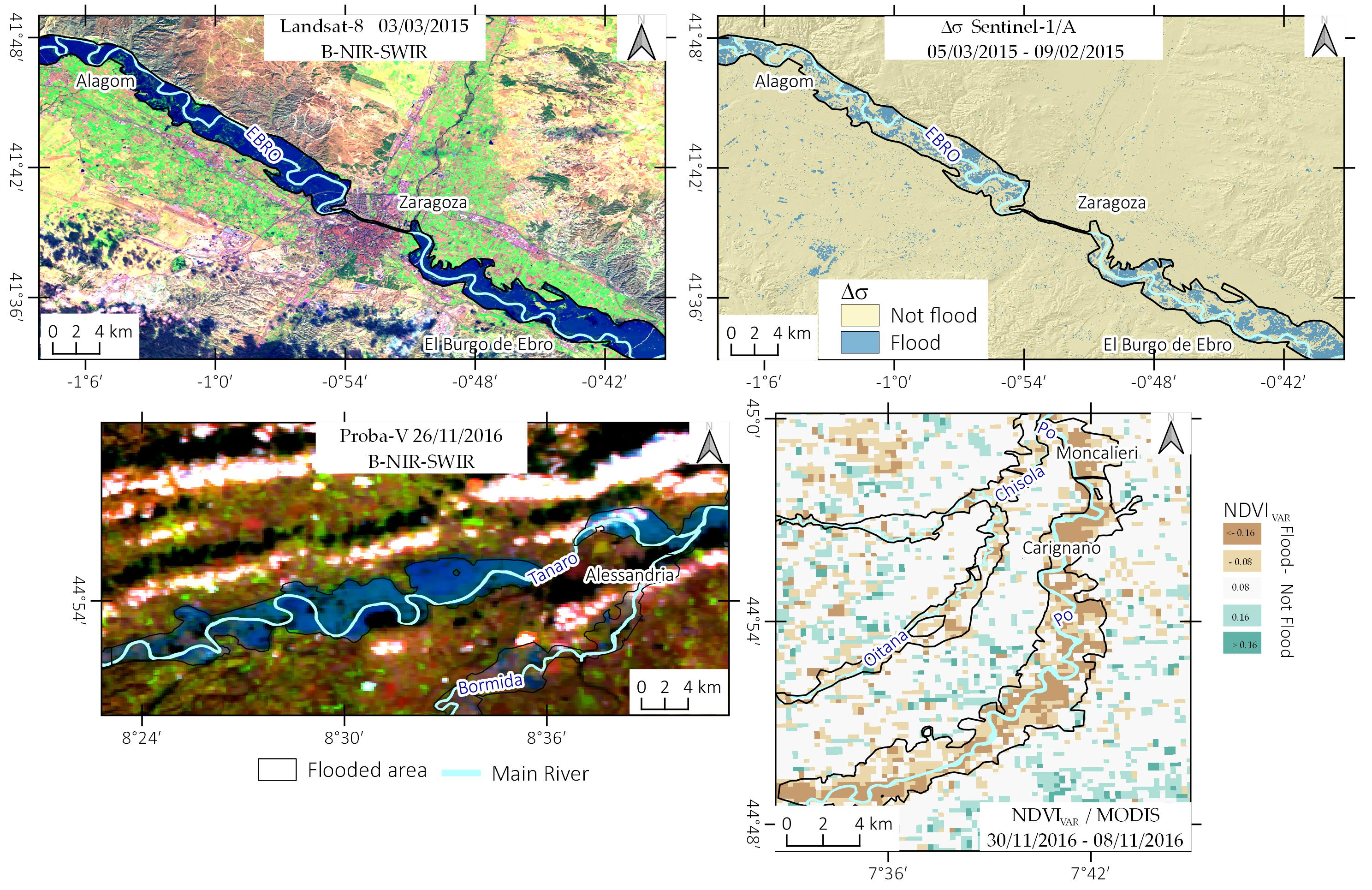
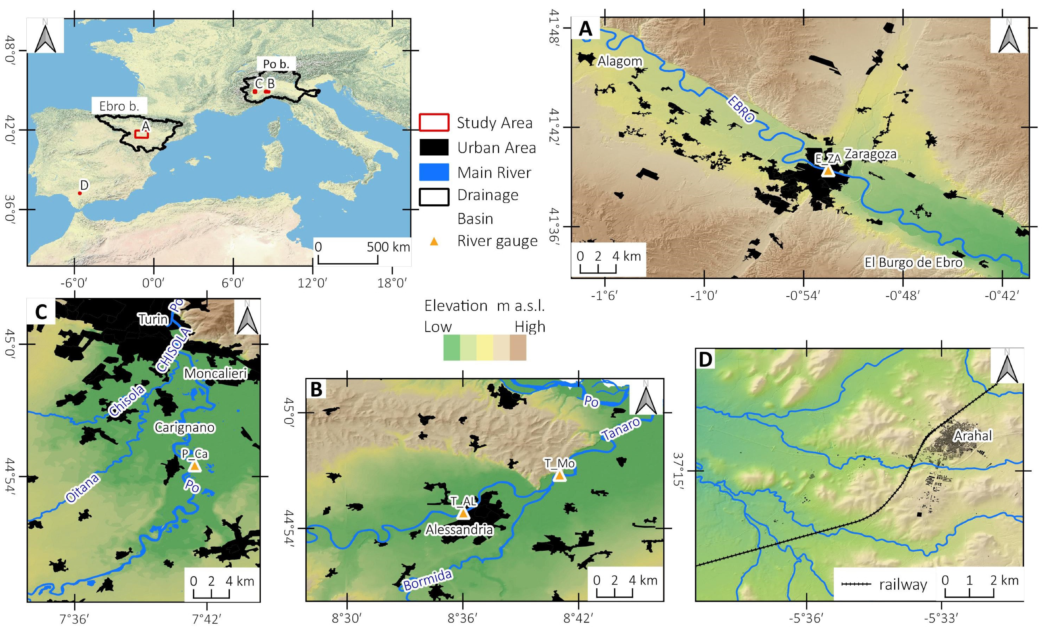
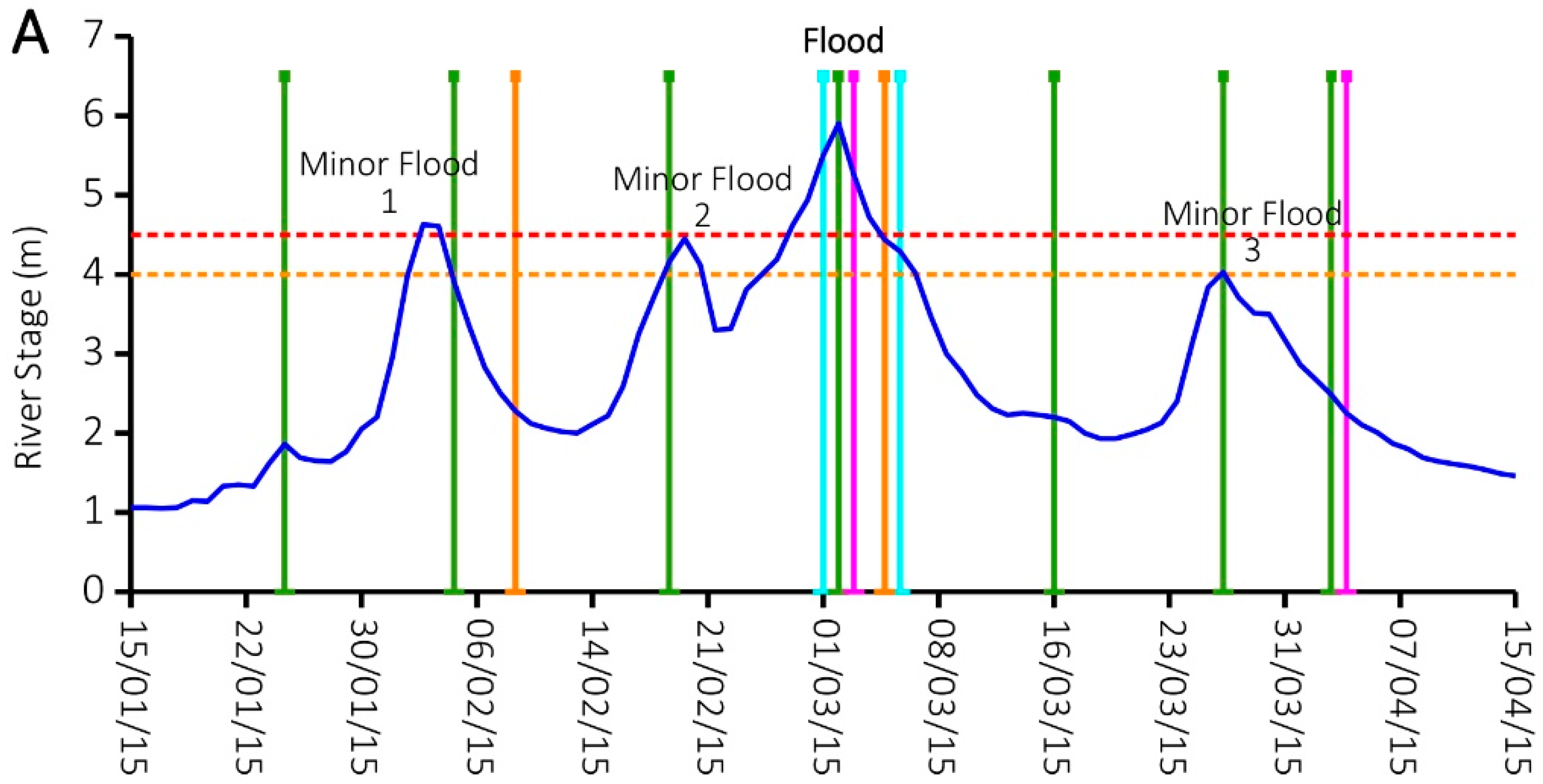
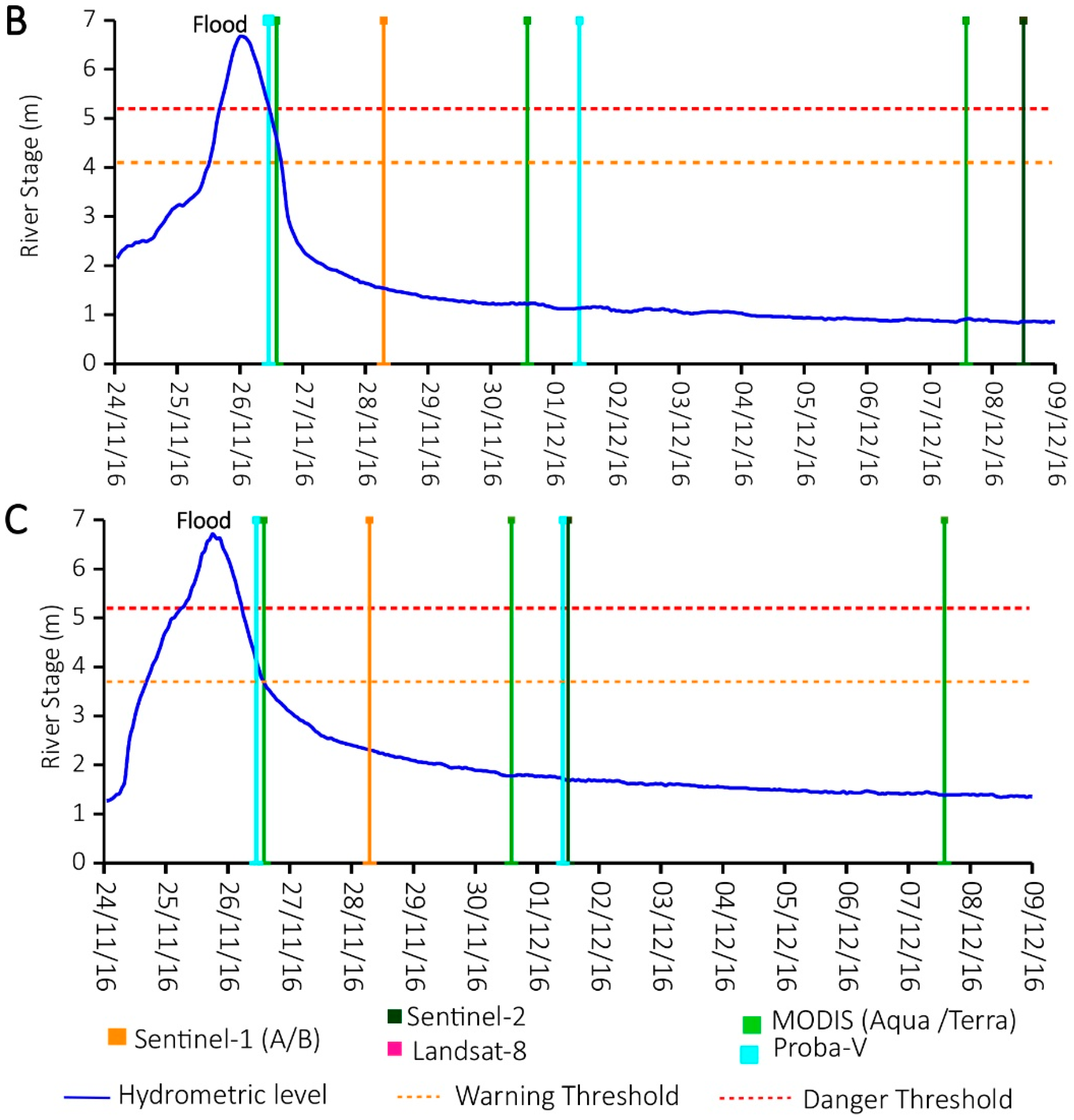
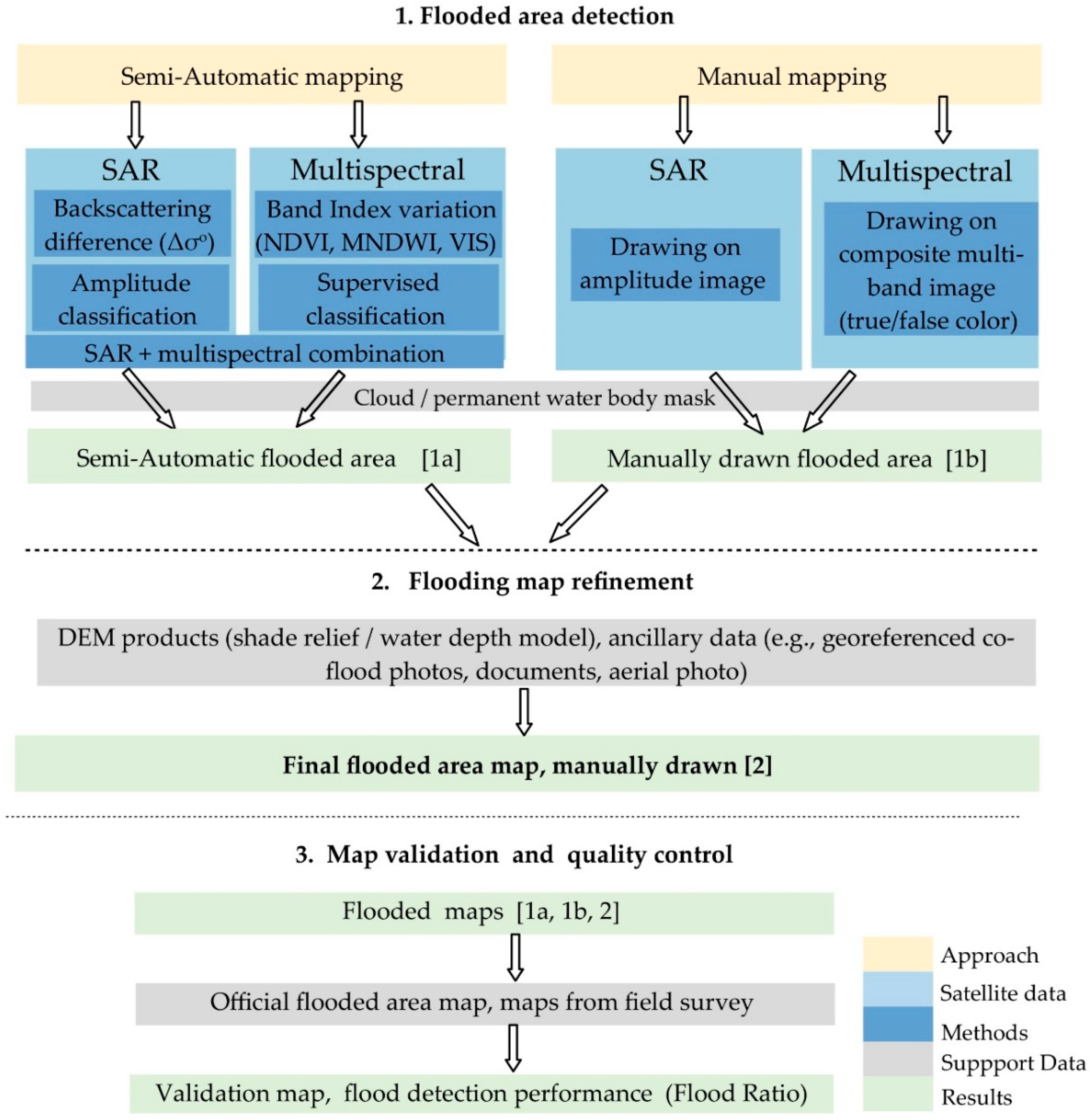
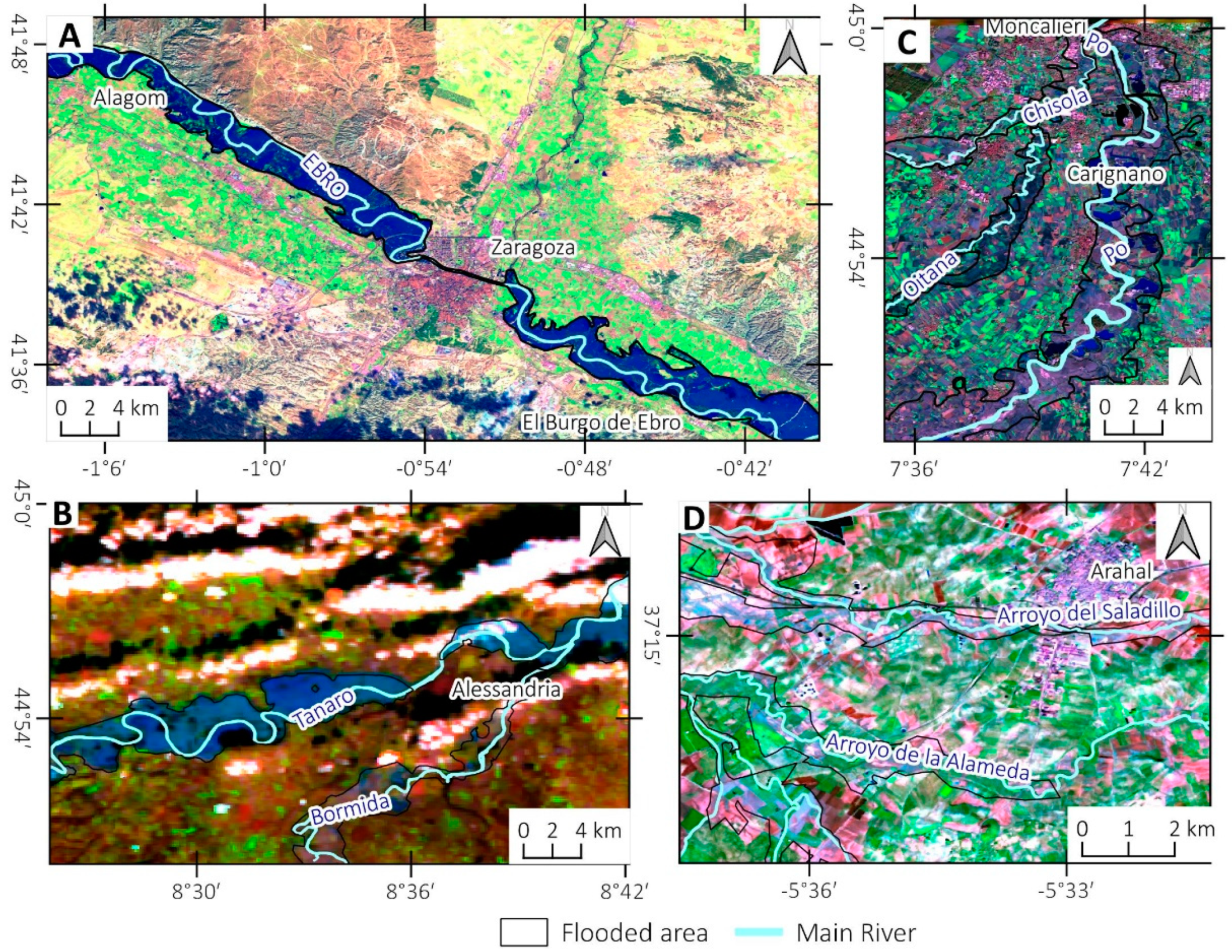
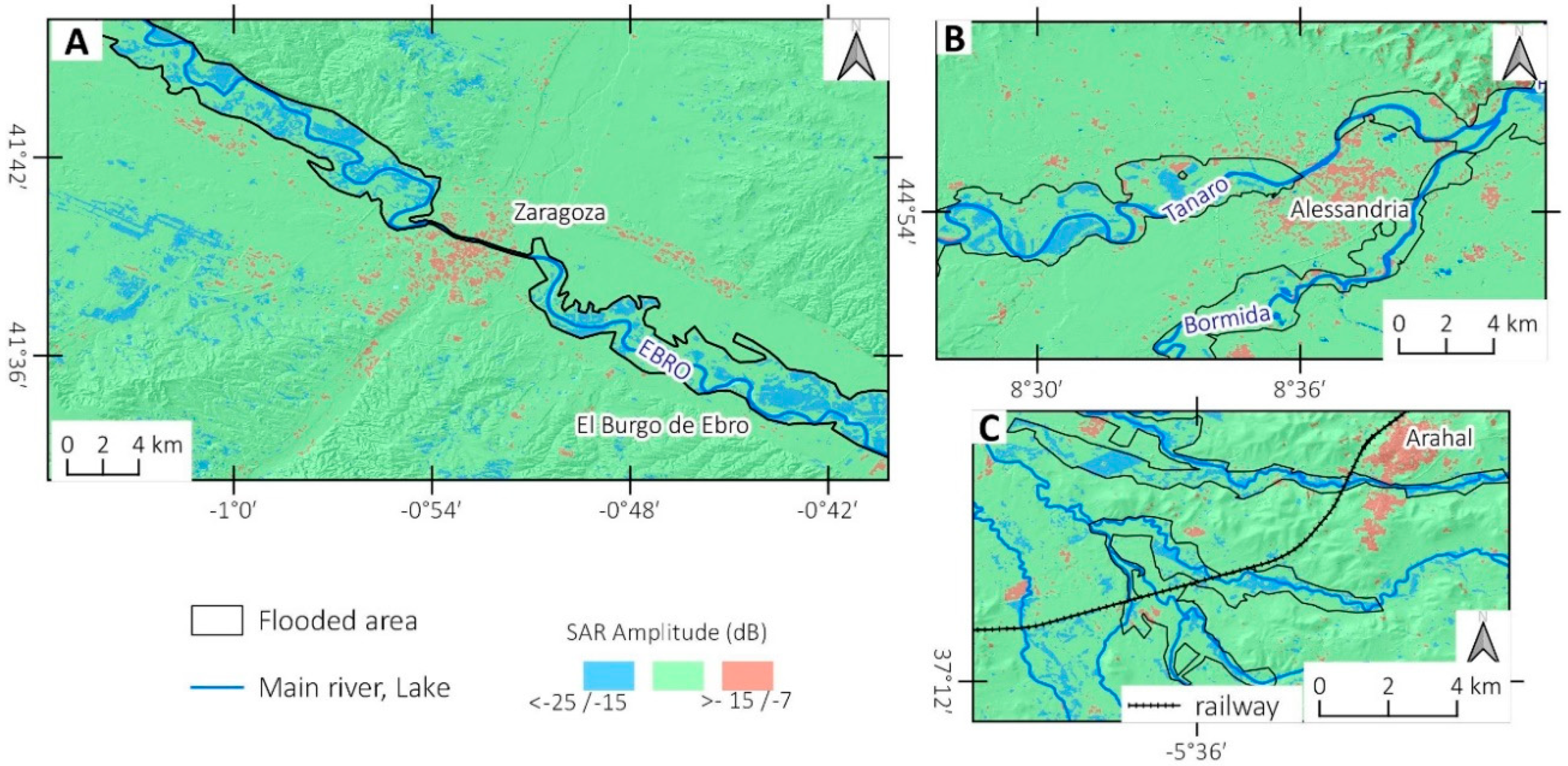
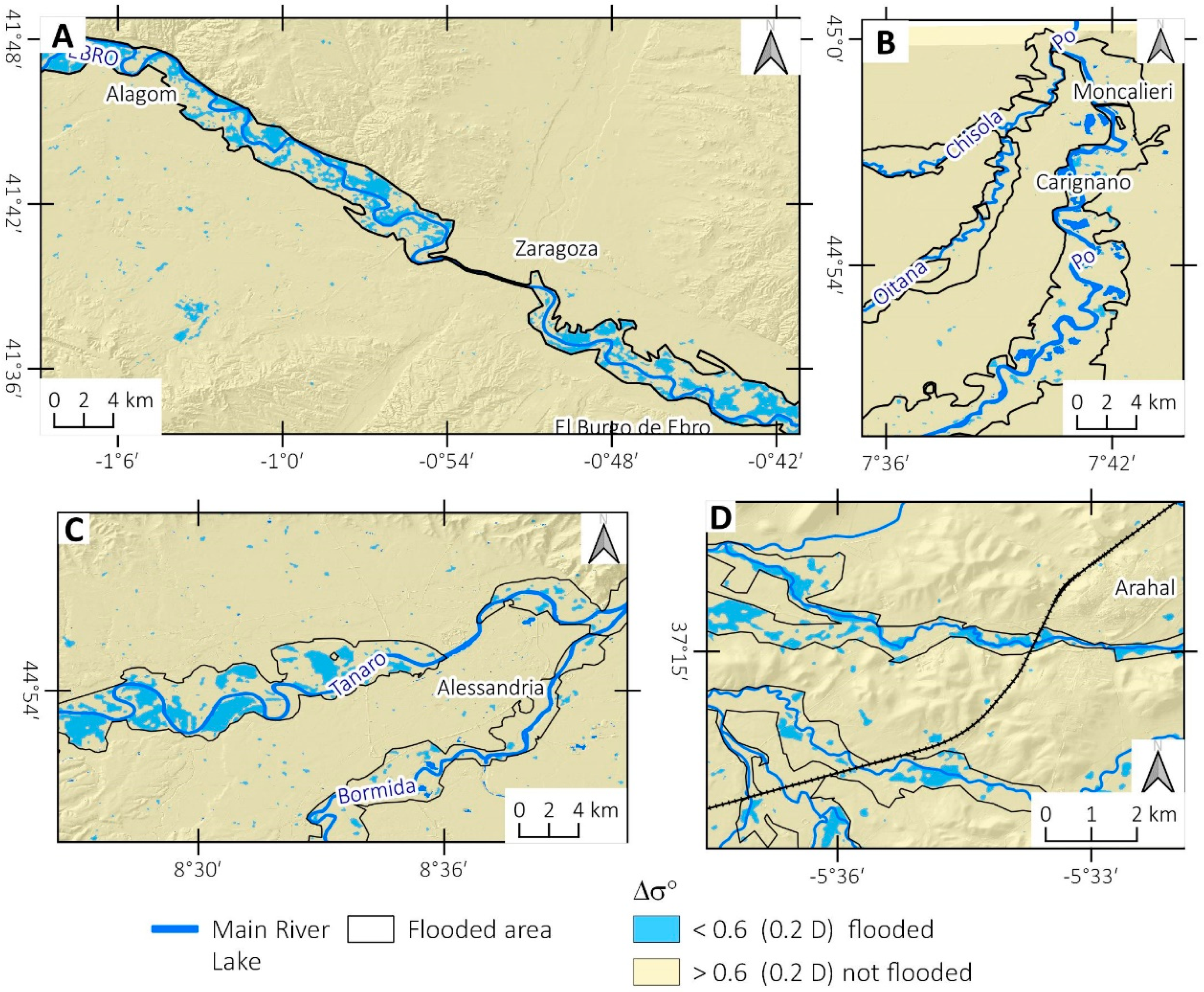
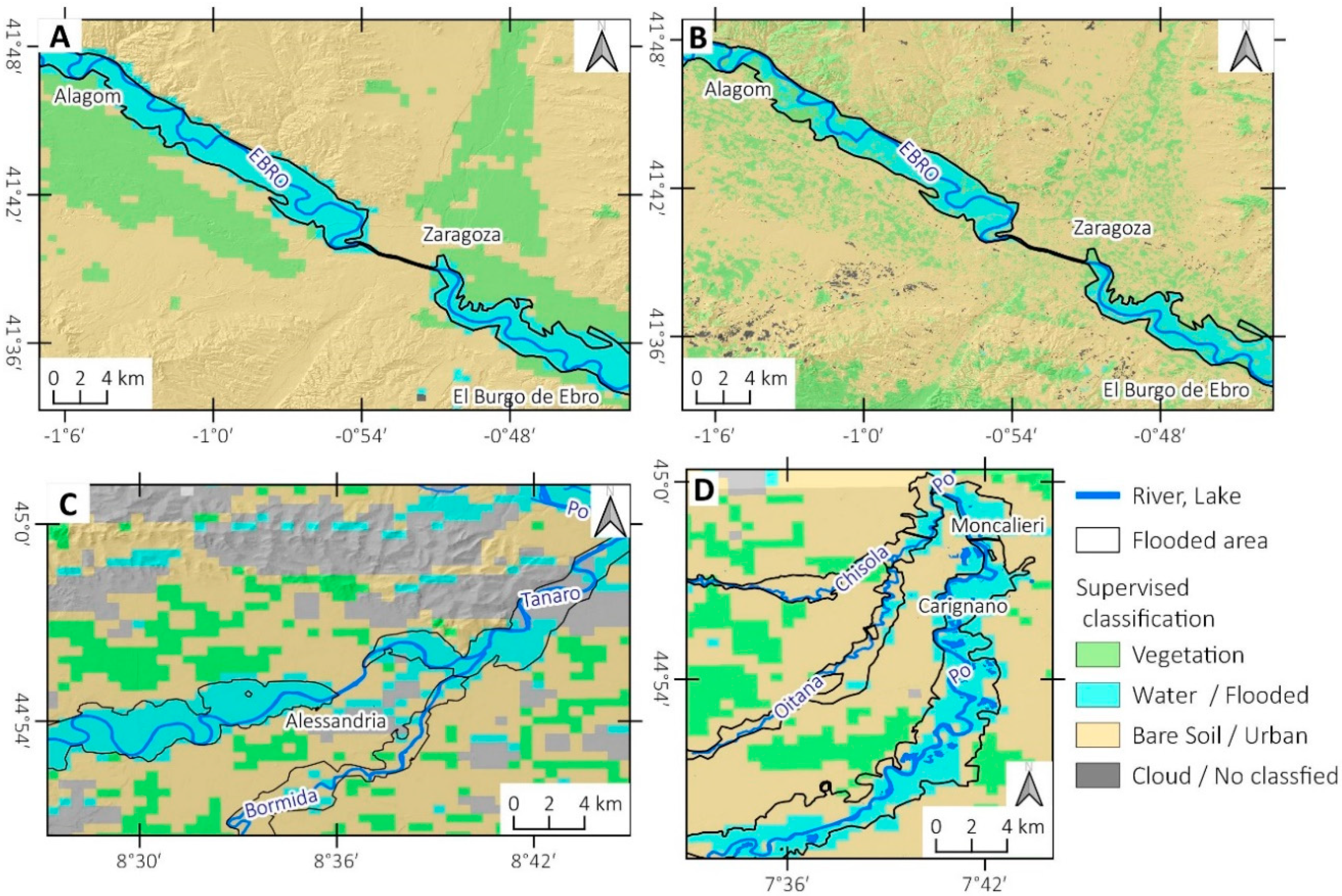
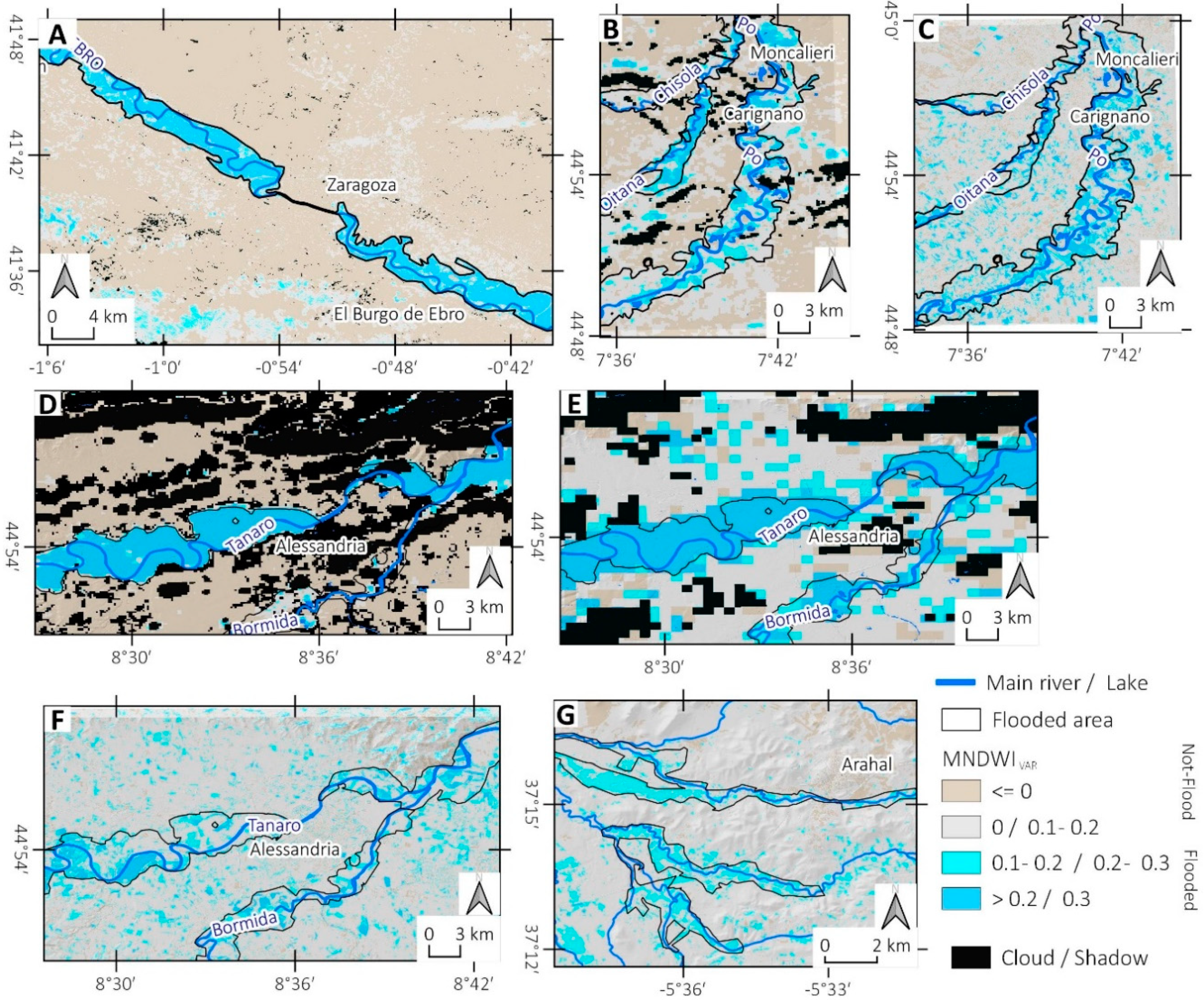
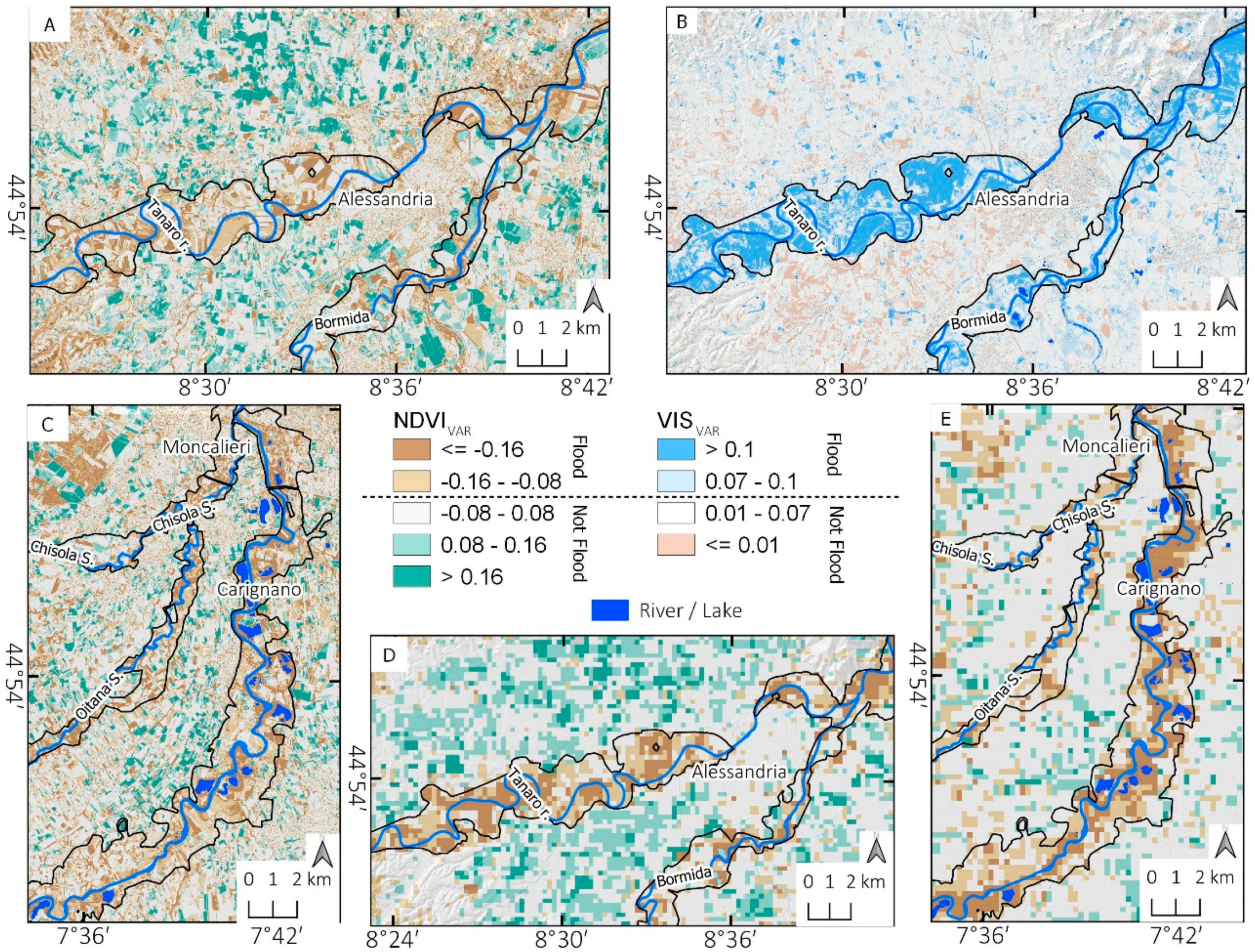
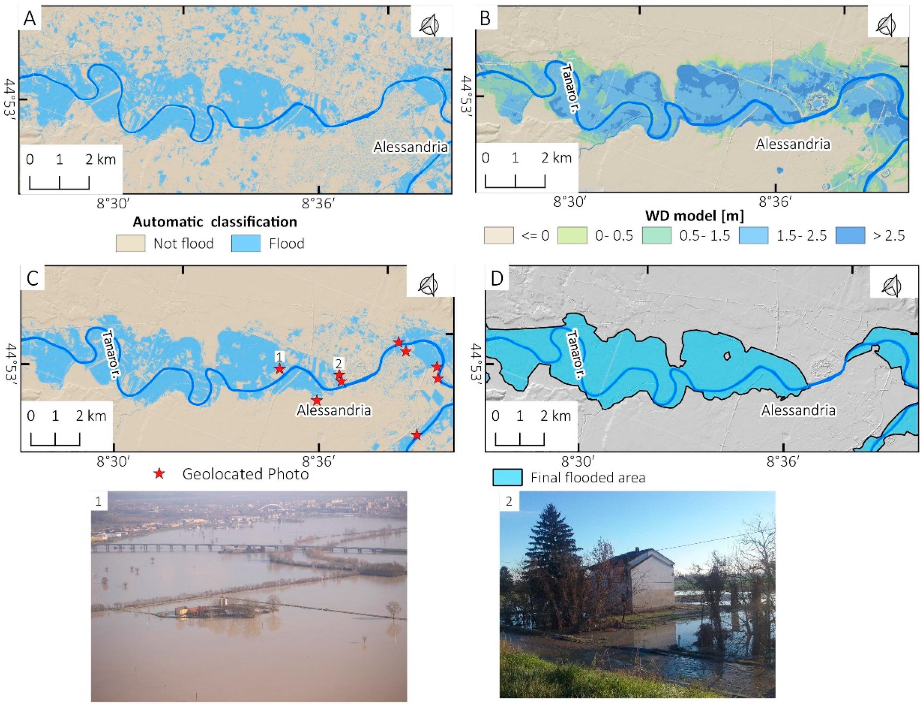
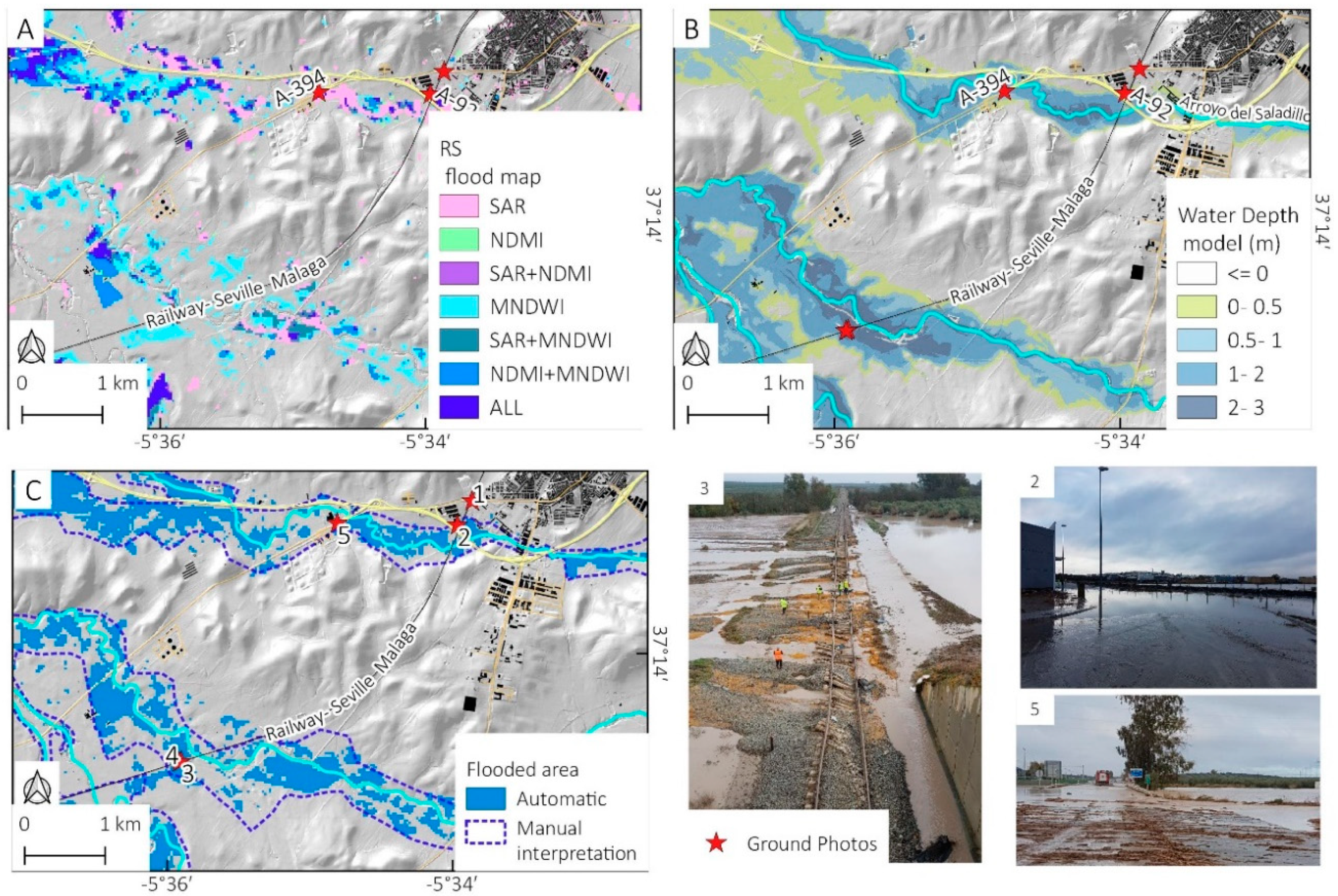
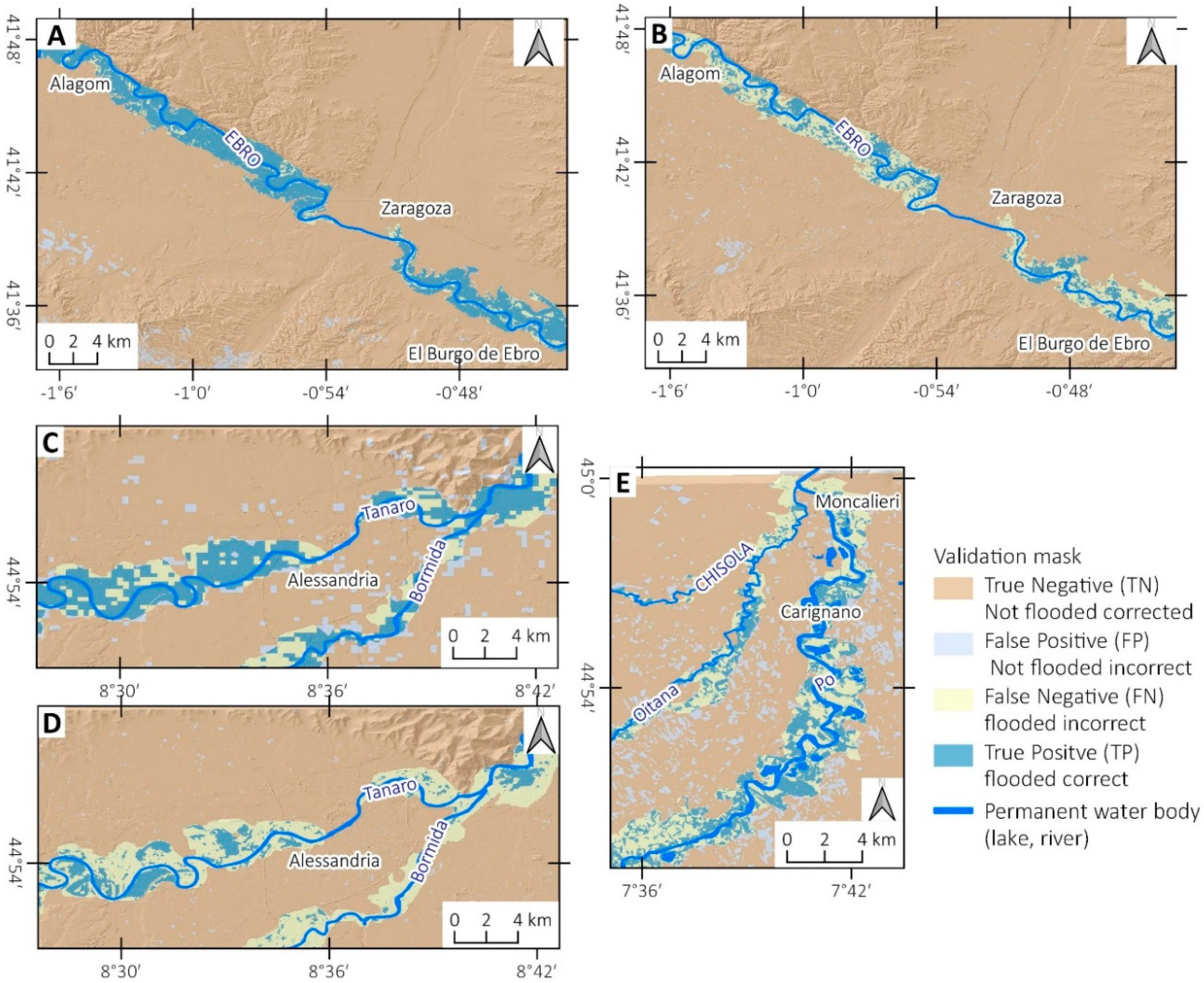
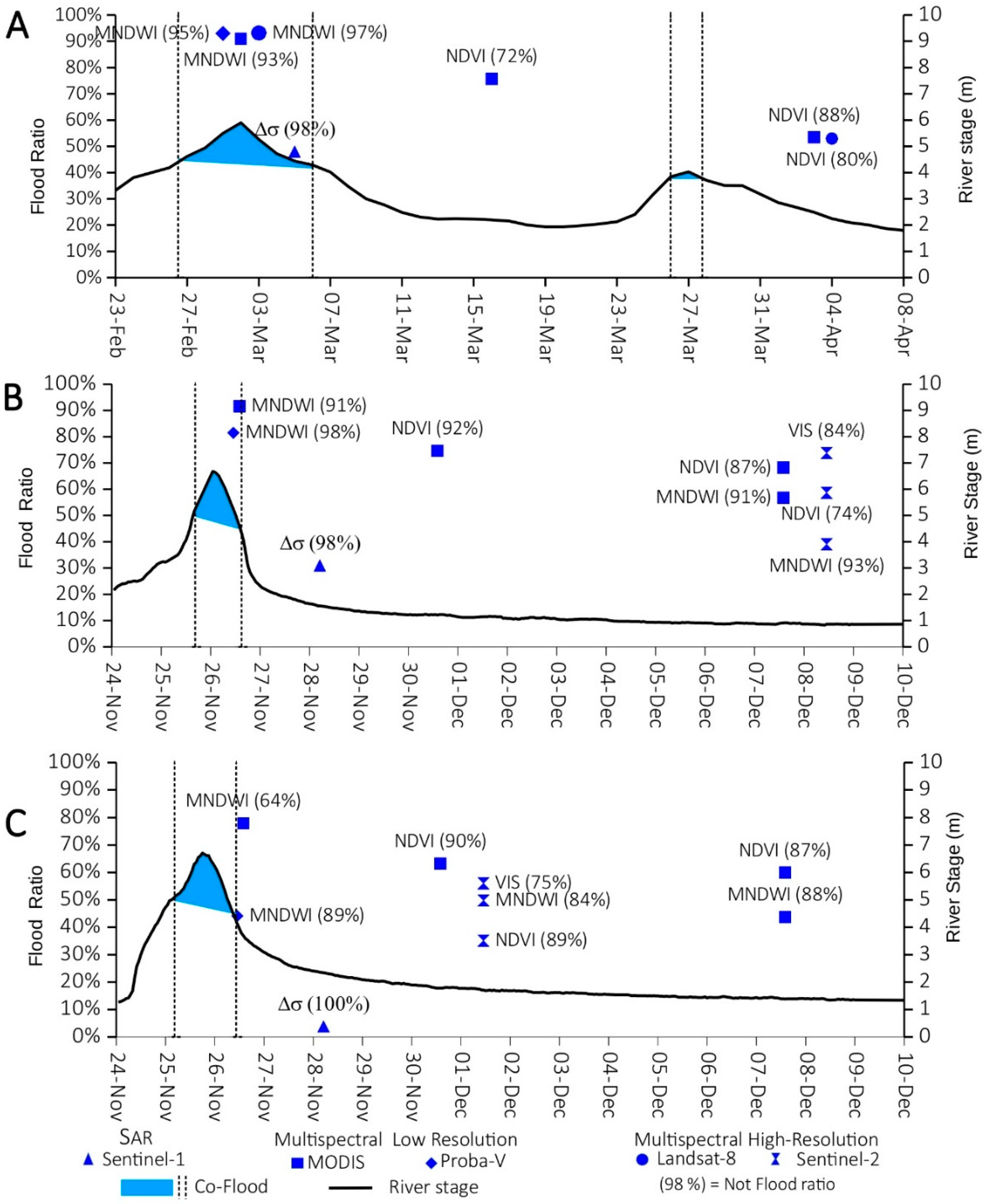
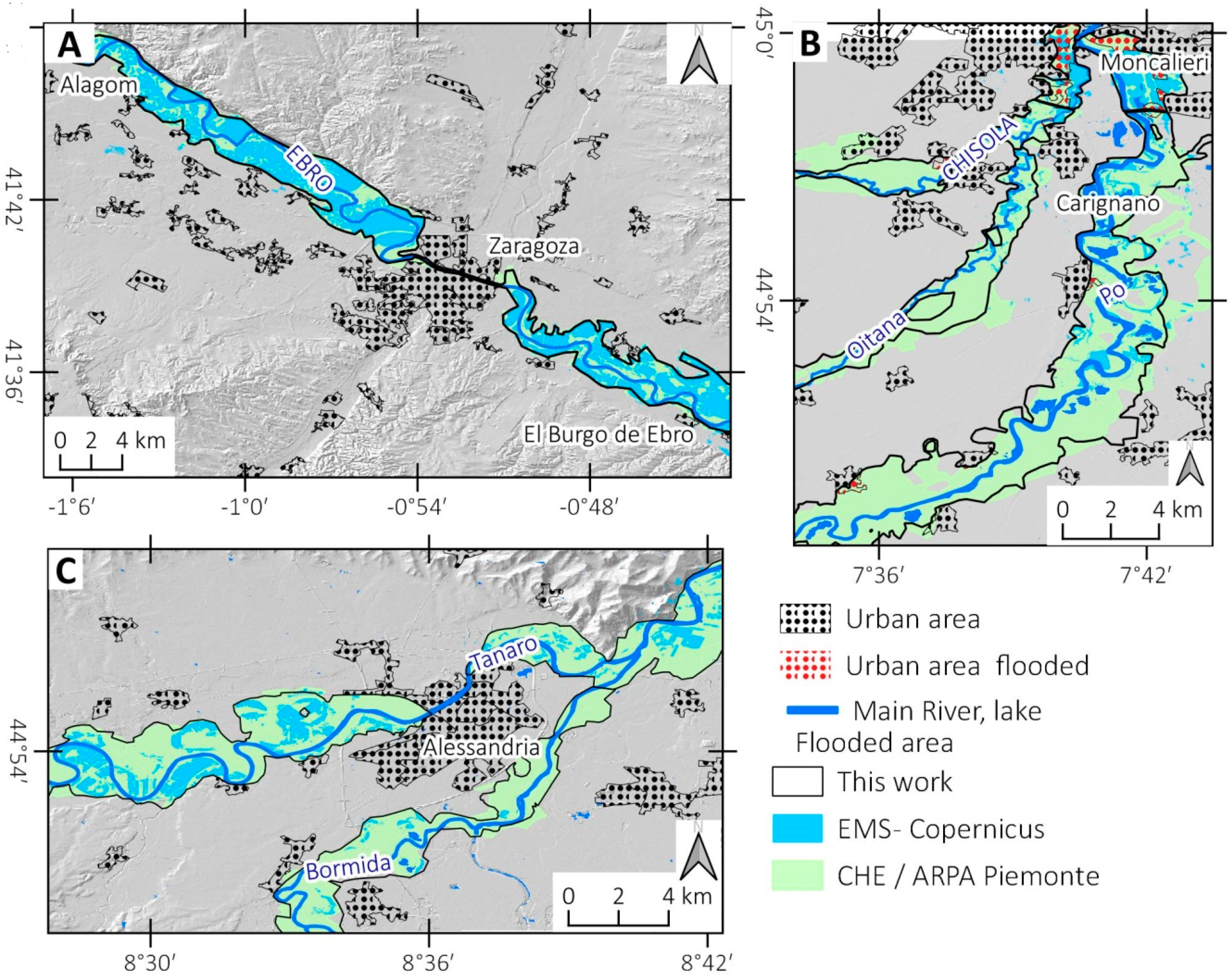
Table 1.
Characteristics of the data used in our study.
| Satellite | Band Used | Spatial Resolution (m) | Revisit Time (Day) | Data Availability |
|---|---|---|---|---|
| MODIS-Terra/Aqua | R; G; B; NIR; SWIR(2) | 250 ÷ 500 | 1 | [69] |
| Proba-V | R; B; NIR; SWIR | 100 ÷ 300 | 5 ÷ 1 | [71] |
| Landsat-8 | R; G; B; NIR; SWIR(2) | 30 | 16 | [72] |
| Sentinel-2 (a/b) | R; G; B; NIR; RE(2); SWIR(2) | 10 ÷ 20 | 5 ÷ 10 | [62] |
| Sentinel-1 (a/b) | C | 5 × 20 (SLC) | 6 ÷ 12 | [62] |
Table 2.
Bans and wavelength used for this study.
| Band Name | Wavelength Interval |
|---|---|
| Blue (B) | ~450–500 nm |
| Green (G) | ~500–620 nm |
| Red (R) | ~620–700 nm |
| Red Edge (RE) | ~700–750 nm |
| Near Infrared (NIR) | ~750–1400 nm |
| Shortwave Infrared (SWIR) | ~1400–3000 nm |
| SAR-Band (C) | ~5 cm |
© 2018 by the authors. Licensee MDPI, Basel, Switzerland. This article is an open access article distributed under the terms and conditions of the Creative Commons Attribution (CC BY) license (http://creativecommons.org/licenses/by/4.0/).
Share and Cite
MDPI and ACS Style
Notti, D.; Giordan, D.; Caló, F.; Pepe, A.; Zucca, F.; Galve, J.P. Potential and Limitations of Open Satellite Data for Flood Mapping. Remote Sens. 2018, 10, 1673. https://0-doi-org.brum.beds.ac.uk/10.3390/rs10111673
AMA Style
Notti D, Giordan D, Caló F, Pepe A, Zucca F, Galve JP. Potential and Limitations of Open Satellite Data for Flood Mapping. Remote Sensing. 2018; 10(11):1673. https://0-doi-org.brum.beds.ac.uk/10.3390/rs10111673
Chicago/Turabian StyleNotti, Davide, Daniele Giordan, Fabiana Caló, Antonio Pepe, Francesco Zucca, and Jorge Pedro Galve. 2018. "Potential and Limitations of Open Satellite Data for Flood Mapping" Remote Sensing 10, no. 11: 1673. https://0-doi-org.brum.beds.ac.uk/10.3390/rs10111673
Note that from the first issue of 2016, this journal uses article numbers instead of page numbers. See further details here.