More Than Meets the Eye: Using Sentinel-2 to Map Small Plantations in Complex Forest Landscapes


School of GeoSciences, Crew Building, The King’s Buildings, University of Edinburgh, Edinburgh EH9 3FF, UK
*
Author to whom correspondence should be addressed.
Remote Sens. 2018, 10(11), 1693; https://0-doi-org.brum.beds.ac.uk/10.3390/rs10111693
Submission received: 17 September 2018
/
Revised: 17 October 2018
/
Accepted: 23 October 2018
/
Published: 26 October 2018
(This article belongs to the Section Forest Remote Sensing)
Abstract
:Many tropical forest landscapes are now complex mosaics of intact forests, recovering forests, tree crops, agroforestry, pasture, and crops. The small patch size of each land cover type contributes to making them difficult to separate using satellite remote sensing data. We used Sentinel-2 data to conduct supervised classifications covering seven classes, including oil palm, rubber, and betel nut plantations in Southern Myanmar, based on an extensive training dataset derived from expert interpretation of WorldView-3 and UAV data. We used a Random Forest classifier with all 13 Sentinel-2 bands, as well as vegetation and texture indices, over an area of 13,330 ha. The median overall accuracy of 1000 iterations was >95% (95.5%–96.0%) against independent test data, even though the tree crop classes appear visually very similar at a 20 m resolution. We conclude that the Sentinel-2 data, which are freely available with very frequent (five day) revisits, are able to differentiate these similar tree crop types. We suspect that this is due to the large number of spectral bands in Sentinel-2 data, indicating great potential for the wider application of Sentinel-2 data for the classification of small land parcels without needing to resort to object-based classification of higher resolution data.
Keywords:
classification; UAV; WorldView; Sentinel-2; palm oil; Random Forest; Myanmar; Google Earth Engine; rubber; betel nut1. Introduction
Land use change in the tropics has a significant impact on the carbon cycle, and thus global climate change, but it is poorly quantified [1,2]. In mitigating climate change through conserving and enhancing forest carbon stocks, monitoring the changes in land cover and land use provides crucial information for policy development and enforcement in areas such as forest conservation, watershed, and environmental protection [2]. While there are sufficient data on deforestation provided by systematic and free-to-use remote sensing [3], what happens to land after deforestation (or the drivers of deforestation) varies by location [4] and there are no global products providing these data, making local classification of the resulting land use necessary for both carbon accounting and policy implementation purposes.
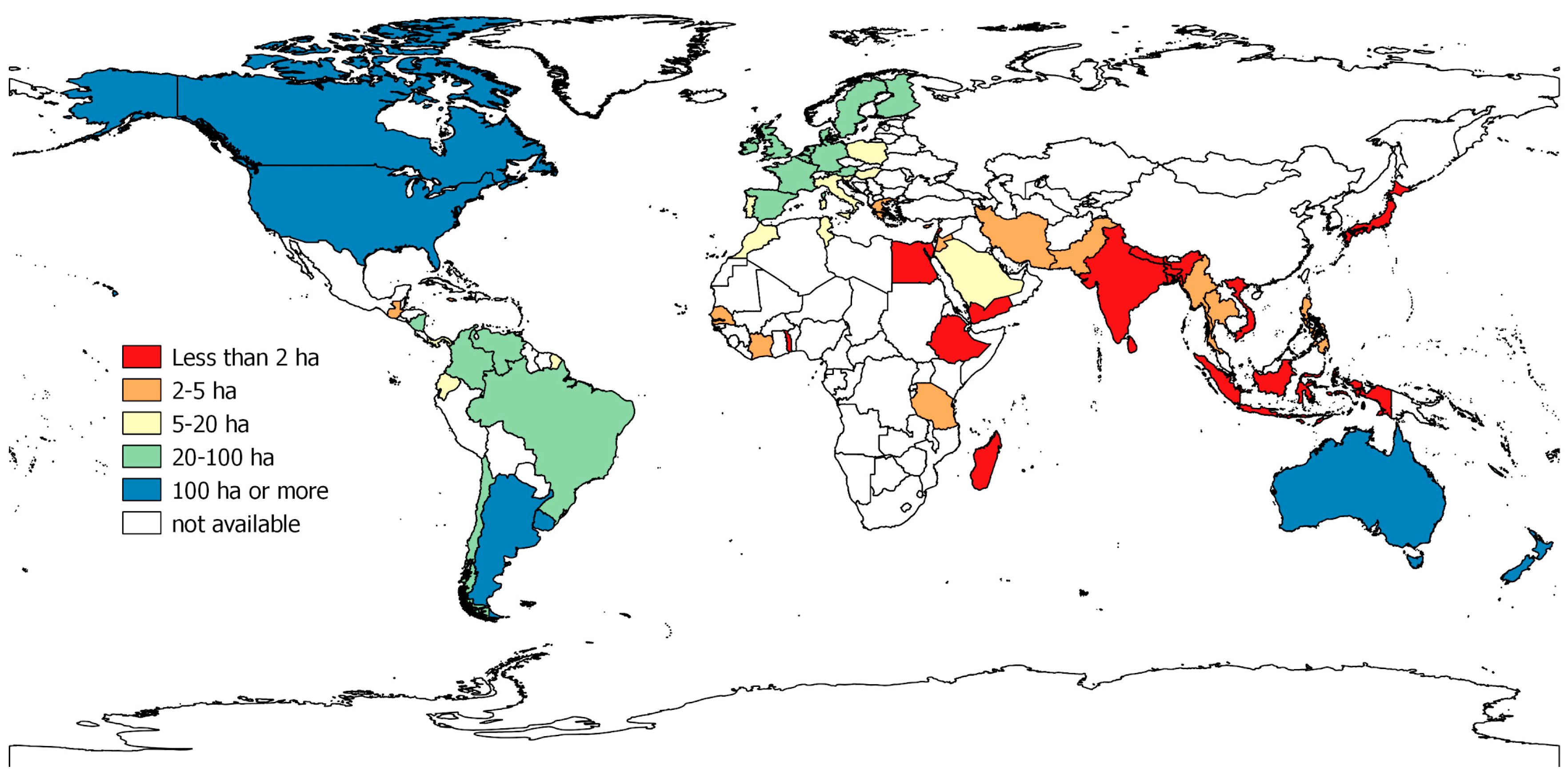
There are a number of ways in which the area of different land cover and land use types within an area, and how they are changing, can be assessed. These range from agricultural census surveys to various types of remote sensing. The most commonly used approaches in the tropics include wall-to-wall mapping using remotely sensed images and/or sample-based approaches for area estimation [5,6,7,8]. However, classifying landscapes can be challenging in the tropics today, as the average farm size has been decreasing in developing countries [9,10]. In Asia, this change has been especially pronounced, with the average size of agricultural holdings falling from 2.5 hectares in 1950 to one hectare in 2000, where the fragmentation of holdings driven by population growth is prevalent (Figure 1) [10,11]. More recently, rubber production has shifted from being dominated by large plantations, to being dominated by smallholders in Southeast Asia, resulting in 80% of global rubber production being managed by smallholders with plantations 2–3 ha in size [12]. To overcome the challenge of this decrease in patch size, high spatial resolution images from unmanned aerial vehicles (UAV, ground resolutions typically 1–50 cm) and hyperspatial satellites such as WorldView-3 (WV3, with the highest resolution band at a 31 cm resolution) can be used, which provide detailed visual information on vegetation on the ground. While these images typically feature few spectral bands (normally optical RGB plus potentially one infrared band), limiting their ability to differentiate land cover types based on spectral characteristics, their high resolution enables the human eye to differentiate most land cover types based on, for example, the shape and density of trees, and the advancement of object-based classification methods has meant that automated processes can also take advantage of this spatial information to produce accurate classifications [13,14,15,16]. However, the high costs and complexity of both the object-based image analysis, and the high cost and low availability of data at a sufficient resolution, remain as challenges for wider application [17,18].
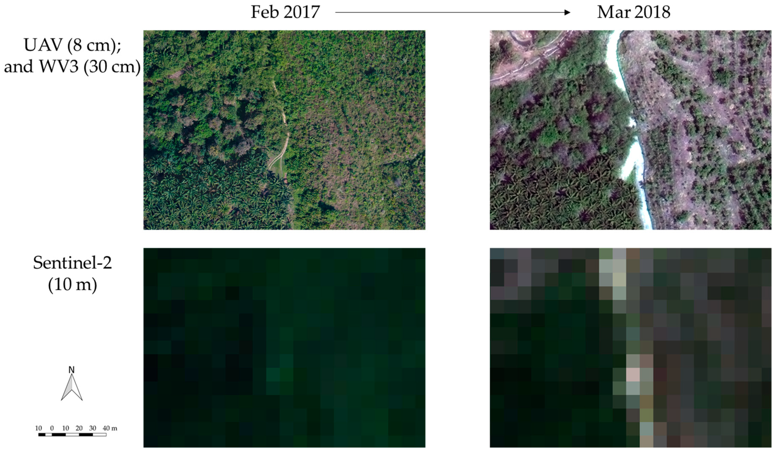
Our study investigated whether publicly available data, namely Sentinel-2 (S2), can map complex landscapes in Southern Myanmar, including oil palm, rubber, and betel nut plantations using a Random Forest classifier on Google Earth Engine. Unlike UAV and WV3 data, widely available satellite data (which is typically at best a 10–30 m resolution, with the standard platforms of Landsat and Sentinel-2) cannot be used to visually detect individual trees (Figure 2). However, Sentinel-2 has great potential for mapping vegetation types in complex landscapes as it is a multispectral instrument with 13 bands, some of which (for example, the ‘red edge’ bands) cover very narrow portions of the spectrum, less than 20 nm wide, giving it some of the advantages in classification that were traditionally only available to a true hyperspectral sensor. The resolutions of the bands vary, with four at a 10 m resolution, and the rest at a 20 or 60 m resolution. Taking advantage of the spectral bands with a 10–20 m pixel size, several studies have estimated the extent of land cover types (e.g., cropland, wetland, snow cover) and produced maps of certain forest types (e.g., savanna, deciduous forests) and urban landscapes [19,20,21,22,23,24]. Furthermore, with a high revisit frequency of five days, agricultural monitoring systems are being developed using Sentinel-2 data, taking advantage of its temporal as well as spectral resolution [25]. However, to our knowledge there has been no attempt to classify a landscape with as complex a mixture of small patches of similar tree crops as our study site in Myanmar using S2 data, despite the prevalence of such landscapes across the tropics. This is likely because hyperspatial images are typically used to conduct such classifications (but over small spatial areas, due to limited data availability and the high cost of purchasing/collecting and processing such data). Furthermore, S2 data, along with other satellite data, are generally considered for and associated with broader scale analyses.
Classification methods using machine learning algorithms such as decisions trees, support vector machines, and Random Forests are becoming more popular because of their high accuracy and ability to process complex datasets and produce good results with large numbers of input classification bands and training points [26,27,28]. Random Forests were selected to classify the S2 data, as it is an algorithm proven to improve the classification accuracy compared to simpler methods, due to its ensemble learning techniques, and it is thus often applied for multispectral and hyperspectral satellite imagery in small areas [28,29,30]. We also incorporated a texture index in the classification, in order to take advantage of the 10 m information in some S2 bands (even though we performed the classification at 20 m, the resolution of most S2 bands), as local texture is known to increase accuracy [14,31].
Mapping using complex machine learning classifier models and many classifier layers requires a large amount of representative datasets to train the classifier while avoiding over-fitting [32,33]. Therefore, the quality and quantity of training samples affect the classification results [32,33,34]. Such samples can be collected from the field or high resolution images, which allows users to see individual trees [33,35]. We used high resolution images from UAV and WorldView-3 to manually delineate reference data through object recognition, producing a dataset with similar characteristics to ground truth points collected in the field, but at a much lower financial and time cost per point.
In summary, the study aimed to answer the following questions: (1) how accurately we can map areas with small plantations with S2 using a Random Forest classifier; and (2) are such maps accurate and consistent enough that they could be used to confidently detect area changes over a 12-month period? Using our sites in Southern Myanmar as a case study, we are proposing a cost-effective, simple, and transparent approach for mapping small plantations in increasingly common and complex landscapes, which can be applied in other parts of Asia and Africa, where this type of landscape and rapid landcover change are prevalent.
2. Materials and Methods
2.1. Study Site
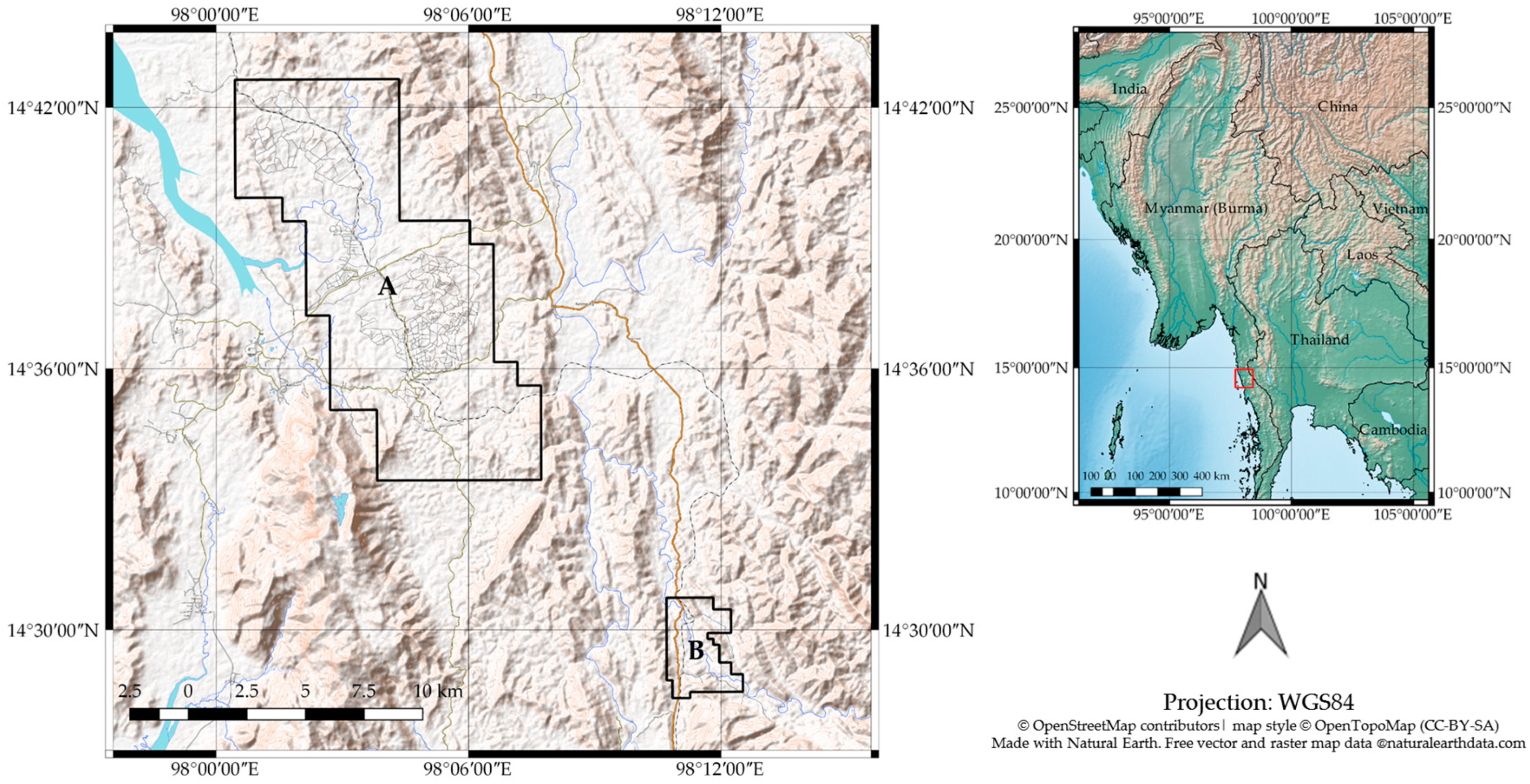
We conducted our analysis in two areas, totaling 13,330 ha, containing oil palm (Elaeis guineensis) plantations in the Dawei district, Tanintharyi region, Myanmar (Figure 3). The Tanintharyi region is in southern Myanmar and west of Thailand, where the development of oil palm plantations started in 1999. Among three districts in the region, Dawei is located to the north, and in general, has older oil palm plantations than those areas to the south. Oil palm companies in this area are believed to be less active, as the dryer climate creates less favourable conditions for oil palm plantations, compared to the other two districts in the south [36]. However, it has been reported that a conflict between villagers and one oil palm company in Area B resulted in a lawsuit in 2016, indicating that there are some actively managed plantations in the area [37].
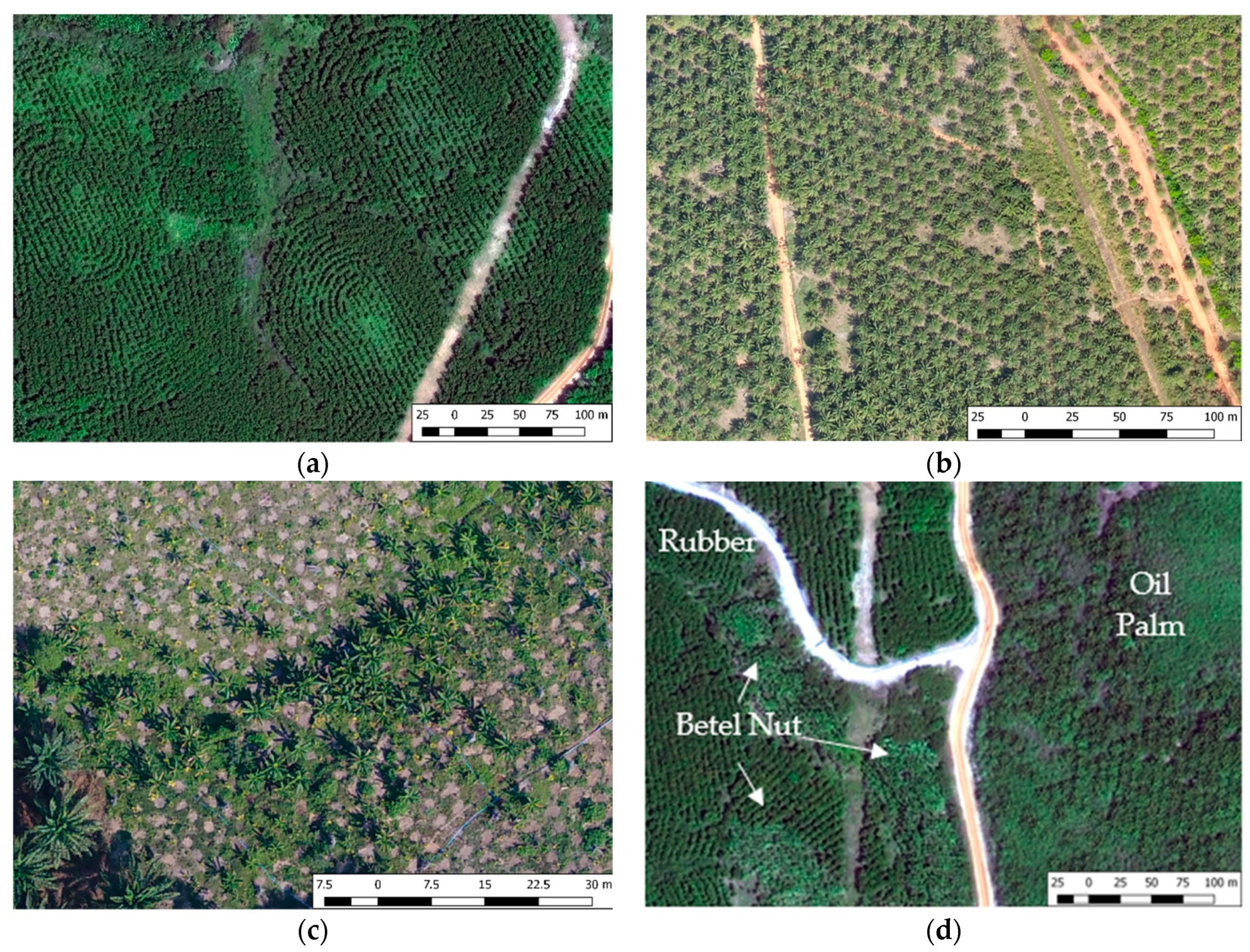
There are two other types of tree crops grown to a significant extent in the area: rubber (Hevea brasiliensis) and betel nut (Areca catechu) plantations. Fortunately all three are planted in different ways and have characteristic shapes, making it possible to distinguish them using hyperspatial remote sensing. Rubber plantations tend to be polygonal in shape with semi-circular portions and each plantation is smaller than an oil palm plantation. At the same time, rubber plantation areas can be large as often there are many plantations established next to each other (Figure 4a), whereas oil palms are typically planted in one large area (Figure 4b). Furthermore, rubber plants tend to be planted in straight lines, while oil palm trees are planted in a triangular form using a 9 m distance between trees. Betel nut trees are slender palm trees with numerous linear leaflets (Figure 4c) [38]. Betel nut plantations are much smaller than the other two crops, and are normally planted in small patches, often abutting or among the other tree crops, along the roads, or between houses. While there are these crop specific plantation styles, they are also seen planted next to each other or in close proximity (Figure 4d).
2.2. Dataset
2.2.1. Sentinel-2 Images for Classification
Sentinel-2 images for the two areas were obtained in Google Earth Engine as image collections within the months of February 2017, and February and March 2018, corresponding to the months when UAV and WV3 images were collected in each area (Table 1). Google Earth Engine allows users to create a single-value composite from a stack of all images collected (an image collection) by selecting the median value of each band for each pixel in the collection. Using images of less than a 10% cloudy pixel to build up the collection ensured that the median composites were cloud free over the set time periods. This was possible because most of the areas had clear images during the study periods. However, a composite for Area A in February 2017 contained clouds in the site when using median values, thus the least cloudy image was used instead of the median values of the images. The code used to process and classify S2 images is available in Supplementary Material.
While certain spectral bands will inevitably be more important than others for the classification, in general, it has been shown that the more spectral bands are included, the better the accuracy, until a certain threshold is reached; following this, the accuracy becomes established [39,40,41,42,43,44,45,46]. Therefore, all of the spectral bands in the Sentinel-2 images were selected to train the classifier (Table 2). In addition, two indices were included: the normalised difference vegetation index (NDVI; Equation (1)) [47] to give the greenness of vegetation; and the standard deviation of NDVI (moving window square 5 × 5 kernel), both calculated at a 10 m resolution. The standard deviation of NDVI gives the texture of greenness, which is commonly used for object-based classification using high resolution images [14,31]. After adding the spectral bands, NDVI, and texture index, the images were scaled to a 20 m spatial resolution.
where NIR is B8 and RED is B4.
2.2.2. Reference Data Points from UAV and WorldView-3
We obtained high resolution images of two areas (12,306 ha and 1024 ha) surrounding oil palm plantations in the Dawei district, Tanintharyi region, Myanmar (Figure 3) [48,49]. The images were collected on 8 and 9 February 2017 by unmanned aerial vehicles (UAV) and on 12 February and 3 March 2018 by WorldView-3 (WV3) in Area A and B, respectively. The UAV images are at approximately an 8 cm spatial resolution and have three spectral bands (red, green, blue), while WV3 images are provided at a 30 cm resolution with four spectral bands, including red, green, and blue, as well as a near infrared (NIR) band (Table 3). The WV3 data is a geometrically- and terrain-corrected pan-sharpened product provided by DigitalGlobe, using the 31 cm resolution panchromatic band to increase the resolution of four of the 1.24 m resolution multispectral bands (RGB and near infrared). The UAV images were processed and mosaicked with Agisoft Photoscan [48]. Both images were georeferenced to the S2 images using the Georeferencer GDAL plug-in on QGIS.
Reference data for training and validation were collected from these images where there were no visible changes in the land cover between the two periods, and where clear images were available. The data were collected according to seven classes of land cover: oil palm, rubber, betel nut, forests (non-plantation, dense tree cover), non-forest (shrubs, regrowth, and other vegetation), bare land, and water. Various plantations in the region were visited from 5 to 25 March 2017 in order to understand the land cover types.
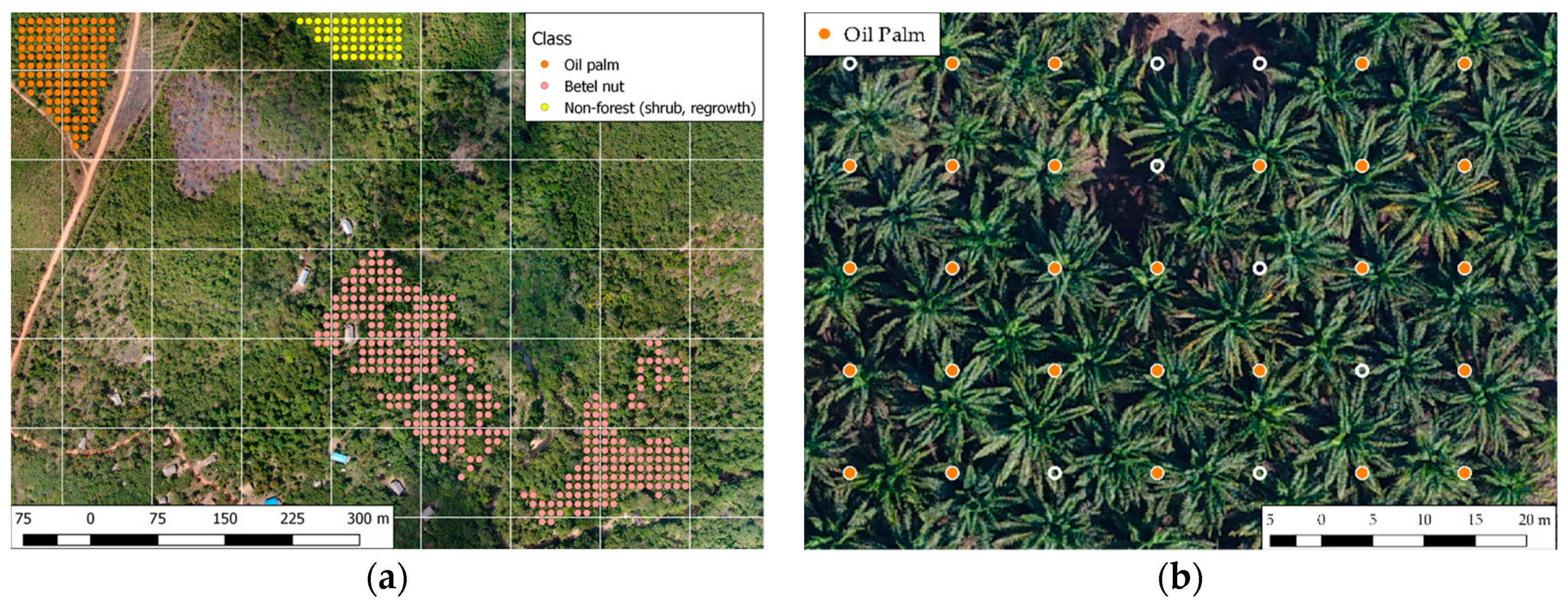
The dot grid photointerpretation method was used in collecting reference data from the hyperspatial imagery (Figure 5) [50,51]. The dot grid method is a traditional approach used by foresters for area estimation [52,53]. We preferred this method over delineating polygons manually because of its systematic nature, lack of subjectivity, and the speed of collecting samples. The dots were systematically superimposed over the images at 10 m intervals. If the dot fell on a certain class, it was collected as reference data of that class (Figure 5a). In the case of oil palm trees, the dot could fall between palm leaflets; in this case, we included that dot as reference data for the oil palm if the dot fell between the leaflets but within the circle connecting the edges of the palm fronds (Figure 5b). Since the classification was performed at 20 m, we avoided collecting samples of different classes that were too close to each other, in order to avoid mixed samples within 20 × 20.
In total, 25,032 reference points (number of dots, placed at 10 m intervals) were collected, among which 50% of the points in each class were randomly selected for training, and the other for accuracy assessment (Table 4). A large number of training points is required when using a machine learning algorithm and a many band multi-spectral image [29,33,34,54]. While there is no literature providing the minimum number of training samples for machine learning algorithms, it has been suggested that the number of features (e.g., wavebands) multiplied by 30 can be used as a guidance [35]. Our samples exceeded this benchmark by 1.5 to 10, except for betel nut plantations in Area B and water class in both areas, which were limited due to the characteristics of the area (limited area of betel nut trees). While there was an attempt to balance the number of points per class, the final set of reference data includes more points for some classes, as it was a result of repeated running of the classifier and the addition of more training data in areas where misclassification was seen to have occurred.
2.3. Random Forest Classification Algorithm
The Random Forest classification utilises ensemble methods with multiple tree-type classifiers [26]. Each tree casts a single vote for the most frequent class to the input data by using a randomly generated subset of input variables for that tree [26,28,29,30]. Therefore, two parameters for the Random Forest classifier had to be set: the number of classification trees; and the number of prediction variables per node (Table 5). As the number of trees increased, the generalization error rate decreased [26,29]. Based on our experiment and considering the computational burden on Google Earth Engine, we selected 30 trees. The number of prediction variables is used at each node to grow the tree, and is generally set at the square root of input variables for classification models like this [28,55]. Therefore, we set the number of variables as four (~the square root of 15). The full Google Earth Engine code used to classify S2 images is available in Supplementary Material.
In addition, we estimated accuracy rates of the maps and the area change between the two time periods [56]. In order to produce robust classification results for area change, the classification of S2 images was run 1000 times by randomly selecting 50% of reference data from each class for training, and testing against the other 50% [57]. The area of each class produced by each run was used to estimate the confidence intervals for the area change.
3. Results
3.1. Classification Accuracy
Using the reference samples from high resolution imagery as training data for a Random Forest classifier with 30 trees and four prediction variables, Sentinel-2 data were able to classify both areas at overall accuracy rates of 95% and higher for all the four images (Figure 6 and Table 6). This overall accuracy figure indicates the proportion of the area mapped correctly [56].
Accuracy rates per class were also consistently high across the classes, with more than 84.7% and 93.5% median accuracy rates for user’s accuracy (UA) and producer’s accuracy (PA), respectively (Table 7 and Table 8). UA is the proportion of the area mapped as a particular class that matches with the testing data, while PA is the proportion of the area that is a particular class in the testing data and is mapped correctly as that class [56]. Excluding water, the highest average accuracy was 98.4% for rubber (PA), while the lowest average was 84.7% for betel nut (UA).
Although the overall accuracy showed that more than 95% of reference data used for validation was correctly classified, by manually investigating the imagery, we found that some areas we knew to be young rubber plantations were classified as shrubs. Furthermore, the areas with dark shadows of trees, rubber plants, or shrubs were sometimes classified as oil palm, along with the edges of rubber plantations or shrubs. Conversely, some oil palm plantations with less shadow contrast (e.g., oil palm plantations that have been poorly weeded and contain shrubs between the trees) were classified as rubber or shrubs. These misclassifications tend to occur more in the larger area (Area A) and also in the area further from the closest reference data.
3.2. Area Change with Sentinel-2
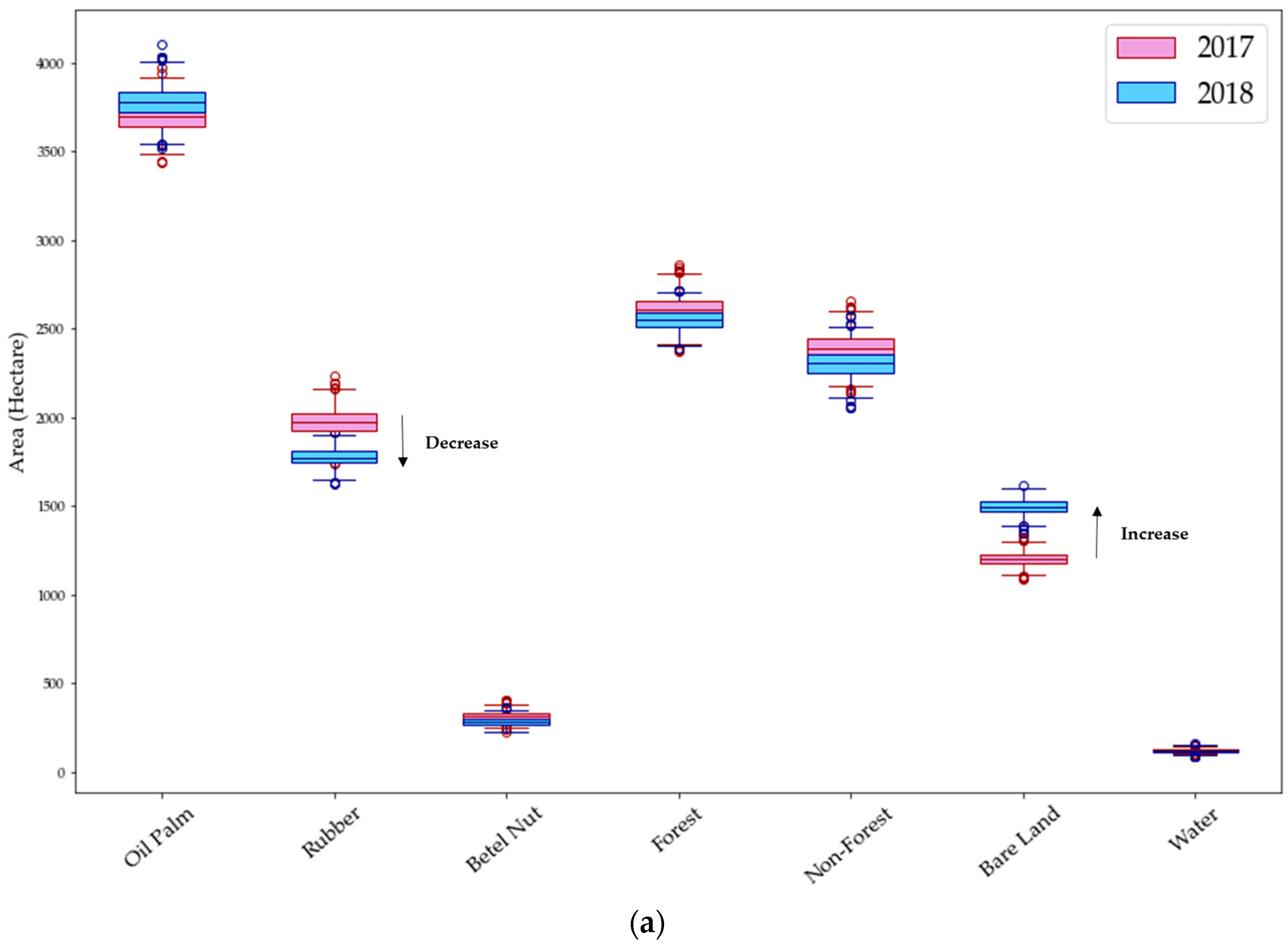
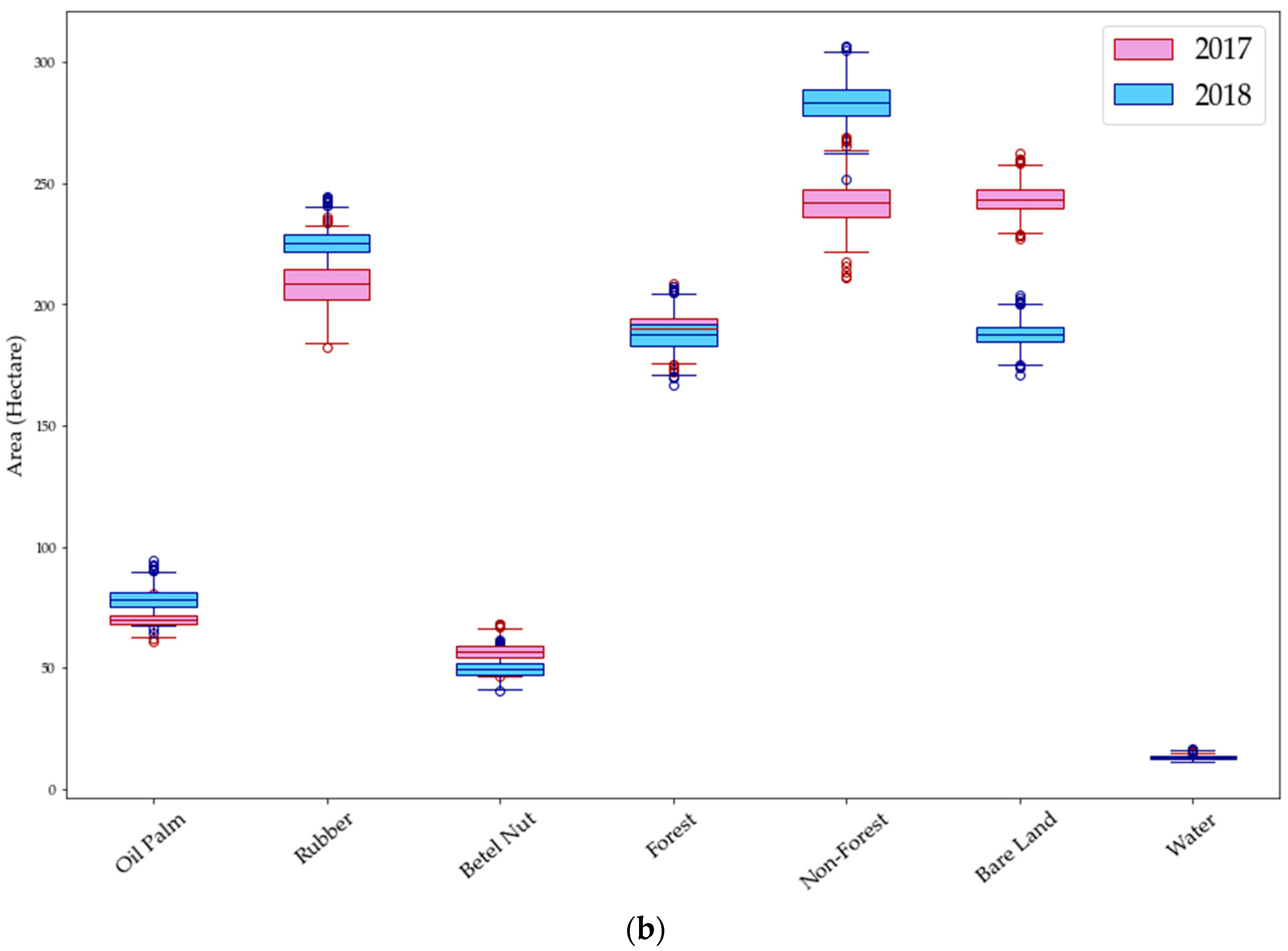
The area changes from 2017 to 2018 were examined by considering the differences between the years, compared to the spread of values from the 1000 iterations. Figure 7 shows boxplots for each area in 2017 and 2018: the median value of the area size (hectare) of each class, the minimum and maximum values, and the 25th and 75th percentiles indicating 50% of the distribution of the data. We considered it likely that there was a significant change if there was no overlap in the interquartile ranges of the two sets of data (represented graphically as no overlap in the box portion of the boxplots in Figure 7). In Area A, the changes were significant for three classes: rubber, betel nut, and bare land. In Area B, most of the classes show differences in area, except for forest and water classes (Figure 7).
Taking the median values of the results, in Area A, bare land increased by 24%. This indicates the clearing of trees between 2017 and 2018, which seems to be accompanied by decreases in betel nut and shrub areas. The rubber plantations also showed a decline of 10%; however, the visual interpretation shows a clear increase of rubber, especially in the south of Area A. This may be due to an overestimation of rubber plantations in 2017, as most of the rubber plantations were young, making them difficult to distinguish from other classes, especially shrubs, resulting in more pixels classified as rubber sporadically across the area, as well as around the edges of various vegetation types.
In Area B, shrub area and oil palm plantations increased by 17% and 11%, respectively. It should be noted that increases in plantations do not indicate planting of the crop between 2017 and 2018, as such new plantations are more likely to be classified as bare land or shrubs. Rather, the increases show the growth of crops that were planted a few years earlier, to the point where they become detectable. The rubber plantations also show an increase of 8%. Similarly to Area A, most of the rubber plantations were young in 2017, and the classified map shows a widespread increase of rubber in 2018. These increases in plantations and shrubs are consistent with a decrease in bare land.
4. Discussion
The main advantage of Sentinel-2 (S2) data is its multispectral instruments with 13 bands, which we believe was the main factor in achieving high accuracy rates (Figure S1). Therefore, for the purpose of classification, it is not necessary to have a spatial resolution sufficient to see individual trees in order to differentiate tree crops. In fact, the level of accuracy achieved in this study (>95%) is higher than the average accuracy rates achieved with hyperspatial images with object-based classification methods [14,15,16].
The high spatial resolution of S2, at 10 to 20 m, should be sufficient to classify even very small plantations, making it the ideal tool for mapping fragmented landscapes. While this study used the 20 m spatial resolution for classification, using lower spatial resolutions will likely achieve an even higher accuracy, depending on the purpose of classification and the type (and size distributions) of plantations in the area. In addition, more texture indices may improve the performance of the classifier.
A close examination of the maps, however, revealed limitations of classification accuracy when classifying a large area. The difficulty in classifying the area without reference data nearby implies that more reference data are necessary. However, adding more data will be limited, depending on the computation capacity of the program used. Therefore, the target area has to be limited to a certain extent, considering the computational burden, time, and labour, when classifying complex landscapes.
Furthermore, the levels of maturity or growth of plantations in the reference data affect the ability of the classifier, as evidenced by the impacts of young rubber plantations in 2017. As young plantations tend to confuse the classifier, it is recommended that the year or area where sufficient reference data with mature plantations are available is selected, and it should be accepted that plantations of particular species will only become visible in the classification after a few years of growth. While it is possible to classify crops like betel nut plantations that exist in small patches made of small trees, it remains as a challenge to classify young plantations themselves.
It is also important to note that the results are sensitive to each and every reference data point, which are entirely based on the judgement and skill of the interpreter. In addition to a priori knowledge of the area, precision and meticulousness in selecting reference data is required, especially when classifying complex landscapes at a high resolution. In this study, reference data were selected from where the interpreter can be certain about the class based on the images and knowledge of the area. Therefore, by excluding the areas with possibly mixed classes where they are difficult to classify, the reported accuracy may be higher than reality. This could be fixed by creating a test dataset from random, rather than a selection of ‘ideal’, points. However, the difficulty here is that error would then exist in the test dataset, confusing the interpretation of results.
5. Conclusions
Sentinel-2 (S2) data can successfully classify complex landscapes with small plantations, forests, and shrubs with more than a 95% overall accuracy against independent test data. While different trees crops are not visibly distinguishable in S2 images, when trained with reference data, S2 can classify small plantations such as rubber and betel nut trees with more than a 94% and 85% accuracy, respectively. However, quantifying the changes between 2017 and 2018 presented a challenge due to the dominance of young rubber plantations in 2017 in these particular study areas. The interpretation of the results is therefore limited to: the increase of bare land in Area A, due to the clearing of betel and rubber trees; and the decrease of bare land in Area B due to the increase of shrubs, oil palm, and rubber plantations, which are likely to have been planted a few years earlier. The results show a contrast in the level of activities in tree clearing and the trend of rubber plantations in two areas.
The accuracy results indicate the strength of Sentinel-2’s multispectral bands in producing accurate classifications of similar land cover classes at a high (20 m) resolution. However, it should be noted that a large amount of reference data is required to classify complex landscapes with confidence, which restricts the size of the area to be classified, given limitations in terms of the collection of training points and the analysis of data.
Supplementary Materials
The following are available online at https://0-www-mdpi-com.brum.beds.ac.uk/2072-4292/10/11/1693/s1: Figure S1: Spectral bands per class; and Google Earth Engine code for classification using Sentinel-2 (S2) data with reference data from UAV and WV3 for February 2017 and February and March 2018 in Areas A and B.
Author Contributions
All authors contributed to the conceptualization of the study and funding acquisition. K.N. conducted the analysis under the supervision of E.T.A.M.
Funding
This research was funded by the Elizabeth Sinclair Irvine Bequest and Centenary Agroforestry 89 Fund from the University of Edinburgh, the Royal Geographical Society’s Henrietta Hutton Research Grant, and NERC grant NE/M021998/1 and ERC grant 757526 (FODEX) to E.T.A.M. K.N. is supported by the Japan Student Services Organization’s postgraduate scholarship for overseas education.
Acknowledgments
We would like to thank OneMap Myanmar, Fauna and Flora International, and Zaw Win for invaluable insights into oil palm plantations in Myanmar; and Phyu Phyu San and Thazin Nwe for their invaluable assistance in the field. We also would like to thank Matthew Hansen from the University of Maryland for facilitating an interesting discussion on our research, and Alexandra Tyukavina for her advice on reference data collection. Lastly, many thanks to Jakob Assmann and Genevieve Patenaude for their help and advice, including their suggestions for the title.
Conflicts of Interest
The authors declare no conflict of interest.
References
- Mitchard, E.T. The tropical forest carbon cycle and climate change. Nature 2018, 559, 527. [Google Scholar] [CrossRef] [PubMed]
- Grassi, G.; House, J.; Dentener, F.; Federici, S.; den Elzen, M.; Penman, J. The key role of forests in meeting climate targets requires science for credible mitigation. Nat. Clim. Chang. 2017, 7, 220. [Google Scholar] [CrossRef]
- Hansen, M.C.; Potapov, P.V.; Moore, R.; Hancher, M.; Turubanova, S.A.; Tyukavina, A.; Thau, D.; Stehman, S.V.; Goetz, S.J.; Loveland, T.R.; et al. High-resolution global maps of 21st-century forest cover change. Science 2013, 342, 850–853. [Google Scholar] [CrossRef] [PubMed]
- Zarin, D.J.; Harris, N.L.; Baccini, A.; Aksenov, D.; Hansen, M.C.; Azevedo-Ramos, C.; Azevedo, T.; Margono, B.A.; Alencar, A.C.; Gabris, C.; et al. Can carbon emissions from tropical deforestation drop by 50% in 5 years? Glob. Chang. Biol. 2016, 22, 1336–1347. [Google Scholar] [CrossRef] [PubMed]
- Till, N. From Reference Levels to Results Reporting: REDD+ under the UNFCCC; Forests and Climate Change Working Paper 15; Food and Agriculture Organization (FAO): Rome, Italy, 2017. [Google Scholar]
- Bartholome, E.; Belward, A.S. GLC2000: A new approach to global land cover mapping from Earth observation data. Int. J. Remote Sens. 2005, 26, 1959–1977. [Google Scholar] [CrossRef]
- Gibbs, H.K.; Ruesch, A.S.; Achard, F.; Clayton, M.K.; Holmgren, P.; Ramankutty, N.; Foley, J.A. Tropical forests were the primary sources of new agricultural land in the 1980s and 1990s. Proc. Natl. Acad. Sci. USA 2010, 107, 16732–16737. [Google Scholar] [CrossRef] [PubMed] [Green Version]
- Mayaux, P.; Holmgren, P.; Achard, F.; Eva, H.; Stibig, H.J.; Branthomme, A. Tropical forest cover change in the 1990s and options for future monitoring. Philos. Trans. R. Soc. Lond. B Biol. Sci. 2005, 360, 373–384. [Google Scholar] [CrossRef] [PubMed] [Green Version]
- Lowder, S.K.; Skoet, J.; Raney, T. The number, size, and distribution of farms, smallholder farms, and family farms worldwide. World Dev. 2016, 87, 16–29. [Google Scholar] [CrossRef]
- FAO. Analysis and International Comparison of the Results (1996–2005); FAO Statistical Development Series 13; Food and Agriculture Organization (FAO): Rome, Italy, 2013. [Google Scholar]
- Masters, W.A.; Djurfeldt, A.A.; De Haan, C.; Hazell, P.; Jayne, T.; Jirström, M.; Reardon, T. Urbanization and farm size in Asia and Africa: Implications for food security and agricultural research. Glob. Food Secur. 2013, 2, 156–165. [Google Scholar] [CrossRef]
- Derek, B.; Deininger, K. The Rise of Large Farms in Land-Abundant Countries: Do They Have a Future. In Land Tenure Reform in Asia and Africa; Palgrave Macmillan: London, UK, 2013; pp. 333–353. [Google Scholar]
- Li, D.; Ke, Y.; Gong, H.; Li, X. Object-based urban tree species classification using bi-temporal WorldView-2 and WorldView-3 images. Remote Sens. 2015, 7, 16917–16937. [Google Scholar] [CrossRef]
- Feng, Q.; Liu, J.; Gong, J. UAV remote sensing for urban vegetation mapping using random forest and texture analysis. Remote Sens. 2015, 7, 1074–1094. [Google Scholar] [CrossRef]
- Amini, S.; Homayouni, S.; Safari, A.; Darvishsefat, A.A. Object-based classification of hyperspectral data using Random Forest algorithm. Geo-Spat. Inf. Sci. 2018, 21, 127–138. [Google Scholar] [CrossRef] [Green Version]
- Su, T.; Zhang, S. Local and global evaluation for remote sensing image segmentation. ISPRS J. Photogramm. Remote Sens. 2017, 130, 256–276. [Google Scholar] [CrossRef]
- Ma, L.; Li, M.; Ma, X.; Cheng, L.; Du, P.; Liu, Y. A review of supervised object-based land-cover image classification. ISPRS J. Photogramm. Remote Sens. 2017, 130, 277–293. [Google Scholar] [CrossRef]
- Georganos, S.; Grippa, T.; Vanhuysse, S.; Lennert, M.; Shimoni, M.; Kalogirou, S.; Wolff, E. Less is more: Optimizing classification performance through feature selection in a very-high-resolution remote sensing object-based urban application. GISci. Remote Sens. 2018, 55, 221–242. [Google Scholar] [CrossRef]
- Immitzer, M.; Vuolo, F.; Atzberger, C. First experience with Sentinel-2 data for crop and tree species classifications in central Europe. Remote Sens. 2016, 8, 166. [Google Scholar] [CrossRef]
- Xiong, J.; Thenkabail, P.S.; Tilton, J.C.; Gumma, M.K.; Teluguntla, P.; Oliphant, A.; Congalton, R.G.; Yadav, K.; Gorelick, N. Nominal 30-m cropland extent map of continental Africa by integrating pixel-based and object-based algorithms using sentinel-2 and Landsat-8 data on Google earth engine. Remote Sens. 2017, 9, 1065. [Google Scholar] [CrossRef]
- Laurin, G.V.; Puletti, N.; Hawthorne, W.; Liesenberg, V.; Corona, P.; Papale, D.; Chen, Q.; Valentini, R. Discrimination of tropical forest types, dominant species, and mapping of functional guilds by hyperspectral and simulated multispectral Sentinel-2 data. Remote Sens. Environ. 2016, 176, 163–176. [Google Scholar] [CrossRef] [Green Version]
- Paul, F.; Winsvold, S.H.; Kääb, A.; Nagler, T.; Schwaizer, G. Glacier remote sensing using sentinel-2. Part II: Mapping glacier extents and surface facies, and comparison to Landsat 8. Remote Sens. 2016, 8, 575. [Google Scholar] [CrossRef]
- De Oliveira Silveira, E.M.; de Menezes, M.D.; Júnior, F.W.; Terra, M.C.; de Mello, J.M. Assessment of geostatistical features for object-based image classification of contrasted landscape vegetation cover. J. Appl. Remote Sens. 2017, 11, 036004. [Google Scholar] [CrossRef]
- Opaloğlu, R.H.; Sertel, E.; Musaoğlu, N. Assessment of Classification Accuracies of SENTINEL-2 and LANDSAT-8 Data for Land Cover/Use Mapping. ISPRS-Int. Arch. Photogramm. Remote Sens. Spat. Inf. Sci. 2016, 41, 1055–1059. [Google Scholar] [CrossRef]
- Sentinel-2 for Agriculture. Available online: http://www.esa-sen2agri.org/ (accessed on 8 August 2018).
- Breiman, L. Random forests. Mach. Learn. 2001, 45, 5–32. [Google Scholar] [CrossRef]
- Mountrakis, G.; Im, J.; Ogole, C. Support vector machines in remote sensing: A review. ISPRS J. Photogramm. Remote Sens. 2011, 66, 247–259. [Google Scholar] [CrossRef]
- Gislason, P.O.; Benediktsson, J.A.; Sveinsson, J.R. Sveinsson. Random forests for land cover classification. Pattern Recognit. Lett. 2006, 27, 294–300. [Google Scholar] [CrossRef]
- Rodriguez-Galiano, V.F.; Ghimire, B.; Rogan, J.; Chica-Olmo, M.; Rigol-Sanchez, J.P. An assessment of the effectiveness of a random forest classifier for land-cover classification. ISPRS J. Photogramm. Remote Sens. 2012, 67, 93–104. [Google Scholar] [CrossRef]
- Pal, M. Random forest classifier for remote sensing classification. Int. J. Remote Sens. 2005, 26, 217–222. [Google Scholar] [CrossRef]
- Laliberte, A.S.; Rango, A. Texture and scale in object-based analysis of subdecimeter resolution unmanned aerial vehicle (UAV) imagery. IEEE Trans. Geosci. Remote Sens. 2009, 47, 761–770. [Google Scholar] [CrossRef]
- Lu, D.; Weng, Q. A survey of image classification methods and techniques for improving classification performance. Int. J. Remote Sens. 2007, 28, 823–870. [Google Scholar] [CrossRef] [Green Version]
- Maxwell, A.E.; Warner, T.A.; Fang, F. Implementation of machine-learning classification in remote sensing: An applied review. Int. J. Remote Sens. 2018, 39, 2784–2817. [Google Scholar] [CrossRef]
- Lu, D.; Mausel, P.; Brondizio, E.; Moran, E. Change detection techniques. Int. J. Remote Sens. 2004, 25, 2365–2401. [Google Scholar] [CrossRef]
- Foody, G.M.; Mathur, A.; Sanchez-Hernandez, C.; Boyd, D.S. Training set size requirements for the classification of a specific class. Remote Sens. Environ. 2006, 104, 1–14. [Google Scholar] [CrossRef]
- Baskett, J.P.C. Myanmar Oil Palm Plantations: A Productivity and Sustainability Review; Fauna & Flora International: Yangon, Myanmar, 2015. [Google Scholar]
- Win, S.P. Homecoming Brings New Cast of Problems for Tanintharyi IDPs. Myanmar Times. 4 October 2016. Available online: www.mmtimes.com/national-news/22880-homecoming-brings-new-cast-of-problems-for-tanintharyi-idps.html (accessed on 1 August 2018).
- Lim, T.K. Areca catechu. In Edible Medicinal and Non-Medicinal Plants; Springer: Dordrecht, The Netherlands, 2012; pp. 260–276. [Google Scholar]
- Lee, J.S.; Wich, S.; Widayati, A.; Koh, L.P. Detecting industrial oil palm plantations on Landsat images with Google Earth Engine. Remote Sens. Appl. Soc. Environ. 2016, 4, 219–224. [Google Scholar] [CrossRef]
- Pal, M.; Mather, P.M. Some issues in the classification of DAIS hyperspectral data. Int. J. Remote Sens. 2006, 27, 2895–2916. [Google Scholar] [CrossRef]
- Sarmah, S.; Kalita, S.K. A Correlation Based Band Selection Approach for Hyperspectral Image Classification. In Proceedings of the 2016 IEEE 6th International Conference on Advanced Computing (IACC), Bhimavaram, India, 27–28 February 2016. [Google Scholar]
- Thenkabail, P.S.; Enclona, E.A.; Ashton, M.S.; Van Der Meer, B. Accuracy assessments of hyperspectral waveband performance for vegetation analysis applications. Remote Sens. Environ. 2004, 91, 354–376. [Google Scholar] [CrossRef]
- Lerma, J.L. Multiband versus multispectral supervised classification of architectural images. Photogramm. Rec. 2001, 17, 89–101. [Google Scholar] [CrossRef]
- De Backer, S.; Kempeneers, P.; Debruyn, W.; Scheunders, P. A band selection technique for spectral classification. IEEE Geosci. Remote Sens. Lett. 2005, 2, 319–323. [Google Scholar] [CrossRef]
- Dalponte, M.; Bruzzone, L.; Vescovo, L.; Gianelle, D. The role of spectral resolution and classifier complexity in the analysis of hyperspectral images of forest areas. Remote Sens. Environ. 2009, 113, 2345–2355. [Google Scholar] [CrossRef]
- Le Bris, A.; Chehata, N.; Briottet, X.; Paparoditis, N. Spectral band selection for urban material classification using hyperspectral libraries. ISPRS Ann. Photogramm. Remote Sens. Spat. Inf. Sci. 2016, 3, 33. [Google Scholar] [CrossRef]
- Tucker, C.J. Red and photographic infrared linear combinations for monitoring vegetation. Remote Sens. Environ. 1979, 8, 127–150. [Google Scholar] [CrossRef] [Green Version]
- Centre for Development and Environment (CDE). OneMap Myanmar; CDE: Yangon, Myanmar, 2017. [Google Scholar]
- DigitalGlobe, Inc. European Space Imaging; DigitalGlobe, Inc.: Munich, Germany, 2018. [Google Scholar]
- Lister, A.; Lister, T.; Doyle, J.A. Use of a simple photointerpretation method with free, online imagery to assess landscape fragmentation. In Proceedings of the 2009 Society of American Foresters National Convention, Opportunities in a Forested World, Orlando, FL, USA, 30 September–4 October 2009. [Google Scholar]
- Nowak, D.J.; Rowntree, R.A.; McPherson, E.G.; Sisinni, S.M.; Kerkmann, E.R.; Stevens, J.C. Measuring and analyzing urban tree cover. Landsc. Urban Plann. 1996, 36, 49–57. [Google Scholar] [CrossRef] [Green Version]
- Barrett, J.P.; Philbrook, J.S. Dot grid area estimates: Precision by repeated trials. J. For. 1970, 68, 149–151. [Google Scholar]
- Bonnor, G.M. The error of area estimates from dot grids. Can. J. For. Res. 1975, 5, 10–17. [Google Scholar] [CrossRef]
- Chen, D.; Stow, D. The effect of training strategies on supervised classification at different spatial resolutions. Photogramm. Eng. Remote Sens. 2002, 68, 1155–1162. [Google Scholar]
- Cutler, D.R.; Edwards, T.C., Jr.; Beard, K.H.; Cutler, A.; Hess, K.T.; Gibson, J.; Lawler, J.J. Random forests for classification in ecology. Ecology 2007, 88, 2783–2792. [Google Scholar] [CrossRef] [PubMed]
- Olofsson, P.; Foody, G.M.; Stehman, S.V.; Woodcock, C.E. Making better use of accuracy data in land change studies: Estimating accuracy and area and quantifying uncertainty using stratified estimation. Remote Sens. Environ. 2013, 129, 122–131. [Google Scholar] [CrossRef]
- Dargie, G.C.; Lewis, S.L.; Lawson, I.T.; Mitchard, E.T.; Page, S.E.; Bocko, Y.E.; Ifo, S.A. Age, extent and carbon storage of the central Congo Basin peatland complex. Nature 2017, 542, 86. [Google Scholar] [CrossRef] [PubMed]
Figure 1.
Average size of agricultural holding in 2000 (data adapted from [9]).
Figure 1.
Average size of agricultural holding in 2000 (data adapted from [9]).

Figure 2.
Examples of images of the same location using UAV, WV3, and Sentinel-2 in February 2017 and March 2018 (shown in RGB).
Figure 2.
Examples of images of the same location using UAV, WV3, and Sentinel-2 in February 2017 and March 2018 (shown in RGB).

Figure 3.
Study sites (A and B) covering oil palm plantations in Dawei district, Tanintharyi, Myanmar. The maps were created with OpenStreetMap contributors (left) and Natural Earth (right).
Figure 3.
Study sites (A and B) covering oil palm plantations in Dawei district, Tanintharyi, Myanmar. The maps were created with OpenStreetMap contributors (left) and Natural Earth (right).

Figure 4.
High resolution imagery of the study sites showing (a) rubber plantations (WV3); (b) oil palm plantation (UAV); (c) betel nut trees in comparison to oil palm trees on the lower left (UAV); (d) all three crops (WV3). UAV images were provided by the Centre for Development and Environment (CDE)—OneMap Myanmar, Yangon, Myanmar; WorldView-3 imagery © 2018 DigitalGlobe, Inc.—provided by European Space Imaging. North is at the top of each image in the figure.

Figure 5.
Dot-grid photointerpretation method showing an example of reference data collected for (a) oil palm, betel nut, and shrub (UAV, Area A, 2017); (b) oil palm trees were identified with orange dots if they fell within the circle of palm canopy (UAV, Area B, 2017).
Figure 5.
Dot-grid photointerpretation method showing an example of reference data collected for (a) oil palm, betel nut, and shrub (UAV, Area A, 2017); (b) oil palm trees were identified with orange dots if they fell within the circle of palm canopy (UAV, Area B, 2017).

Figure 6.
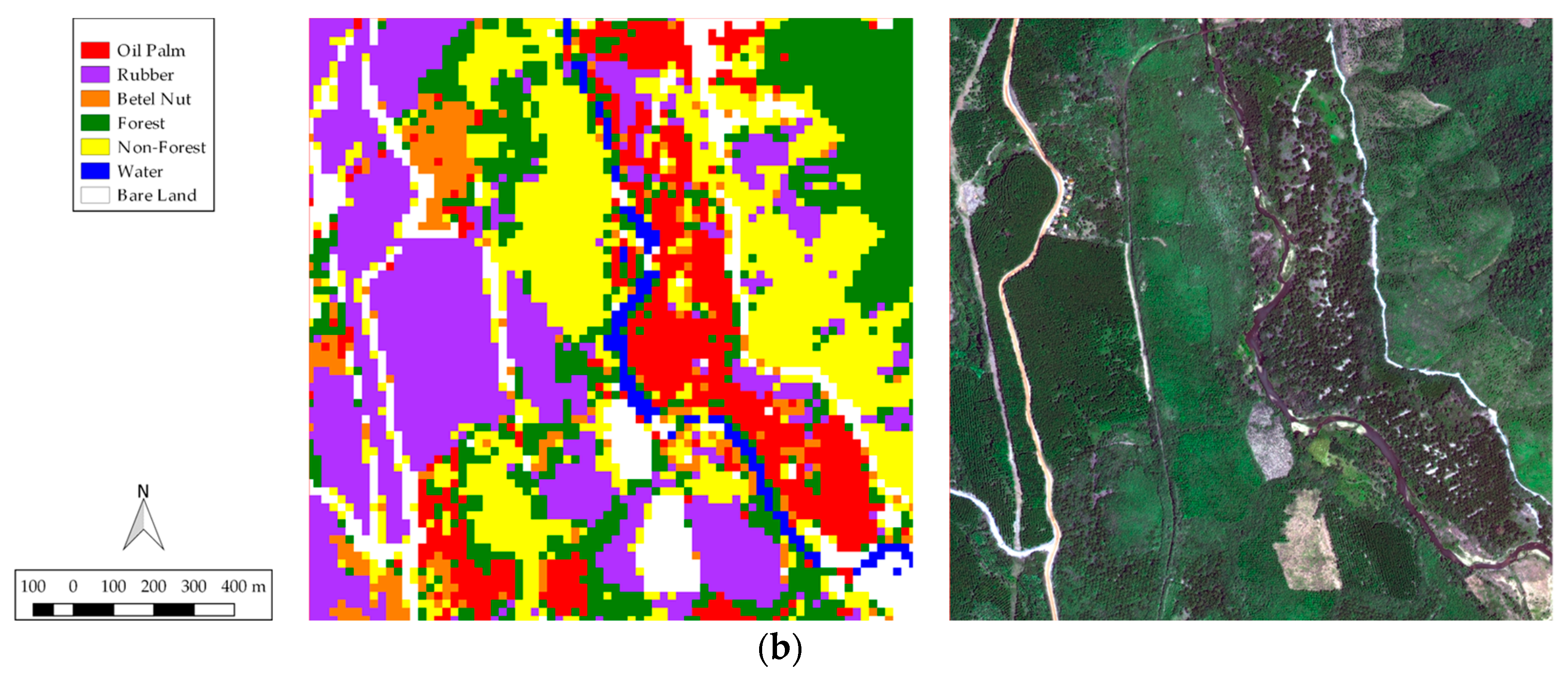
S2 classification results for parts of (a) Area A in February 2017 with the UAV image on the right; (b) Area B in March 2018 with the WV3 image on the right.
Figure 6.
S2 classification results for parts of (a) Area A in February 2017 with the UAV image on the right; (b) Area B in March 2018 with the WV3 image on the right.


Figure 7.
Classification results: area changes by class in (a) Area A; (b) Area B.


Table 1.
Sentinel-2 images used for classification.
| Area | Month Year | Tile | Cloudy Pixel % | Granule ID |
|---|---|---|---|---|
| A | February 2017 | 47PLS | 0 | L1C_T47PLS_A008681_20170219T035623 |
| February 2018 | 47PLS | 9.7756 | L1C_T47PLS_A013829_20180214T040242 | |
| 47PLS | 0 | L1C_T47PLS_A004992_20180219T034801 | ||
| 47PMS | 0.6386 | L1C_T47PMS_A004992_20180219T034801 | ||
| 47PLS | 1.8035 | L1C_T47PLS_A013972_20180224T040129 | ||
| B | February 2017 | 47PMS | 0.3121 | L1C_T47PMS_A008538_20170209T035553 |
| 47PMS | 0 | L1C_T47PMS_A008681_20170219T035623 | ||
| March 2018 | 47PMS | 0.2107 | L1C_T47PMS_A005135_20180301T035914 | |
| 47PMS | 0 | L1C_T47PMS_A014115_20180306T035825 | ||
| 47PMS | 0.0943 | L1C_T47PMS_A014258_20180316T034812 | ||
| 47PMS | 0.0604 | L1C_T47PMS_A005421_20180321T040215 |
Table 2.
Spectral bands in Sentinel-2.
| Name | Resolution | Wavelength | Description |
|---|---|---|---|
| B1 | 60 m | 443.9 nm (S2A)/442.3 nm (S2B) | Aerosols |
| B2 | 10 m | 496.6 nm (S2A)/492.1 nm (S2B) | Blue |
| B3 | 10 m | 560 nm (S2A)/559 nm (S2B) | Green |
| B4 | 10 m | 664.5 nm (S2A)/665 nm (S2B) | Red |
| B5 | 20 m | 703.9 nm (S2A)/703.8 nm (S2B) | Red Edge 1 |
| B6 | 20 m | 740.2 nm (S2A)/739.1 nm (S2B) | Red Edge 2 |
| B7 | 20 m | 782.5 nm (S2A)/779.7 nm (S2B) | Red Edge 3 |
| B8 | 10 m | 835.1 nm (S2A)/833 nm (S2B) | NIR |
| B8a | 20 m | 864.8 nm (S2A)/864 nm (S2B) | Red Edge 4 |
| B9 | 60 m | 945 nm (S2A)/943.2 nm (S2B) | Water vapor |
| B10 | 60 m | 1373.5 nm (S2A)/1376.9 nm (S2B) | Cirrus |
| B11 | 20 m | 1613.7 nm (S2A)/1610.4 nm (S2B) | SWIR 1 |
| B12 | 20 m | 2202.4 nm (S2A)/2185.7 nm (S2B) | SWIR 2 |
Table 3.
Technical specifications of the sensors used in the study and image acquisition dates.
| Sensor | Area | Camera/Sensor | Spatial Resolution | Spectral Bands | Date Acquired |
|---|---|---|---|---|---|
| UAV | A | Phantom 4 Professional built-in camera (20MP, FOV 84°) | 8 cm | 3 (RGB) | 8 February 2017 |
| B | 9 February 2017 | ||||
| WV3 | A | WorldView-3 (4-band pan-sharpened multispectral product) | 30 cm (as provided) | 4 (RGB, NIR) | 12 February 2018 |
| B | 3 March 2018 |
Table 4.
Reference data collected for training and validation.
| Area | Forest | Oil Palm | Rubber | Betel Nut | Non-Forest 1 | Bare Land | Water | Total |
|---|---|---|---|---|---|---|---|---|
| A | 2228 | 4216 | 3191 | 915 | 4881 | 1667 | 303 | 17,401 |
| B | 1588 | 988 | 1577 | 681 | 1257 | 1346 | 194 | 7631 |
| Total | 3816 | 5204 | 4768 | 1596 | 6141 | 3013 | 497 | 25,032 |
1 Shrub, regrowth, other plantations.
Table 5.
Summary of parameters and inputs for Random Forest.
| Random Forest Parameters | INPUT Variables | |
|---|---|---|
| Number of trees | Number of prediction variables per node | Number of variables (Spectral bands and indices) |
| 30 | 4 | 15 (all B bands, NDVI, texture) |
Table 6.
Overall classification accuracy using Sentinel-2 data at a 20 m spatial resolution with 1000 Random Forest classification runs.
Table 6.
Overall classification accuracy using Sentinel-2 data at a 20 m spatial resolution with 1000 Random Forest classification runs.
| Area | Month/Year | Median | 2.5% Bound | 97.5% Bound |
|---|---|---|---|---|
| A | February 2017 | 95.9% | 95.4% | 96.4% |
| February 2018 | 96.0% | 95.5% | 96.5% | |
| B | February 2017 | 95.5% | 94.5% | 96.4% |
| March 2018 | 95.6% | 94.6% | 96.4% |
Table 7.
Median user’s accuracy per class across the four images.
| Area | Month Year | Oil Palm | Rubber | Betel Nut | Forest | Non-Forest 1 | Bare Land | Water |
|---|---|---|---|---|---|---|---|---|
| A | February 2017 | 95.1% | 96.0% | 84.7% | 96.4% | 98.1% | 96.1% | 97.5% |
| February 2018 | 94.8% | 97.1% | 86.8% | 96.9% | 97.8% | 96.1% | 95.9% | |
| B | February 2017 | 94.6% | 95.2% | 93.5% | 97.1% | 94.8% | 97.0% | 94.5% |
| March 2018 | 93.5% | 96.5% | 91.8% | 96.9% | 97.0% | 96.0% | 91.9% |
1 Shrub, regrowth, other vegetation.
Table 8.
Median producer’s accuracy per class across the four images.
| Area | Month Year | Oil Palm | Rubber | Betel Nut | Forest | Non-Forest 1 | Bare Land | Water |
|---|---|---|---|---|---|---|---|---|
| A | February 2017 | 93.8% | 96.6% | 97.5% | 97.0% | 96.1% | 96.4% | 99.4% |
| February 2018 | 94.8% | 98.1% | 98.1% | 96.9% | 96.0% | 94.9% | 99.3% | |
| B | February 2017 | 94.6% | 94.6% | 94.4% | 95.6% | 95.2% | 95.9% | 97.7% |
| March 2018 | 93.5% | 98.4% | 94.1% | 94.5% | 94.0% | 96.9% | 94.0% |
1 Shrub, regrowth, other vegetation.
© 2018 by the authors. Licensee MDPI, Basel, Switzerland. This article is an open access article distributed under the terms and conditions of the Creative Commons Attribution (CC BY) license (http://creativecommons.org/licenses/by/4.0/).
Share and Cite
MDPI and ACS Style
Nomura, K.; Mitchard, E.T.A. More Than Meets the Eye: Using Sentinel-2 to Map Small Plantations in Complex Forest Landscapes. Remote Sens. 2018, 10, 1693. https://0-doi-org.brum.beds.ac.uk/10.3390/rs10111693
AMA Style
Nomura K, Mitchard ETA. More Than Meets the Eye: Using Sentinel-2 to Map Small Plantations in Complex Forest Landscapes. Remote Sensing. 2018; 10(11):1693. https://0-doi-org.brum.beds.ac.uk/10.3390/rs10111693
Chicago/Turabian StyleNomura, Keiko, and Edward T. A. Mitchard. 2018. "More Than Meets the Eye: Using Sentinel-2 to Map Small Plantations in Complex Forest Landscapes" Remote Sensing 10, no. 11: 1693. https://0-doi-org.brum.beds.ac.uk/10.3390/rs10111693
Note that from the first issue of 2016, this journal uses article numbers instead of page numbers. See further details here.