A Comparison between the MODIS Product (MOD17A2) and a Tide-Robust Empirical GPP Model Evaluated in a Georgia Wetland

 , ,
, ,
Abstract
:
1. Introduction
2. Materials and Methods
2.1. Study Site
2.2. Data Sources
2.2.1. MOD17A2
2.2.2. MOD09GA
2.2.3. Flux GPP Data
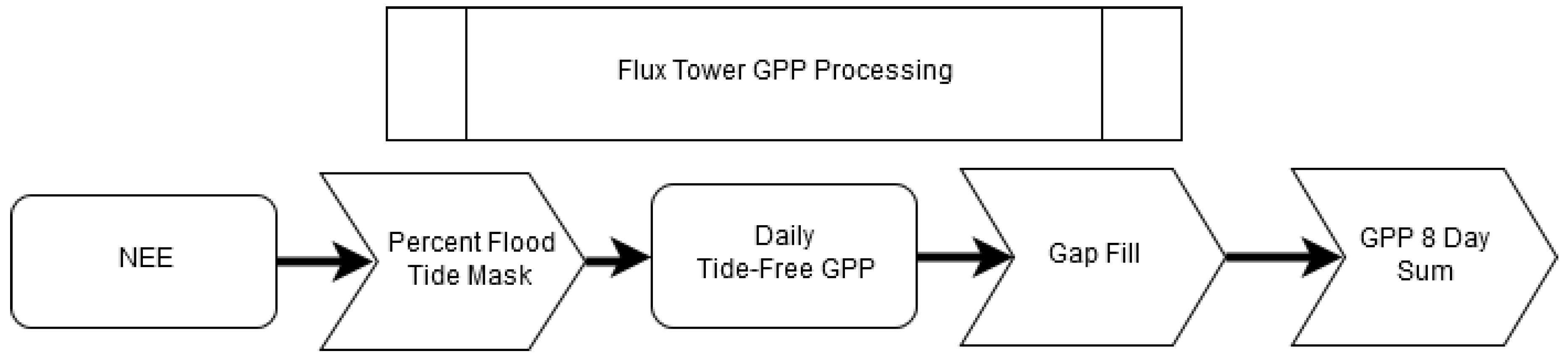
Flux Data Processing
Flux Partitioning
2.2.4. Marsh Inundation Data
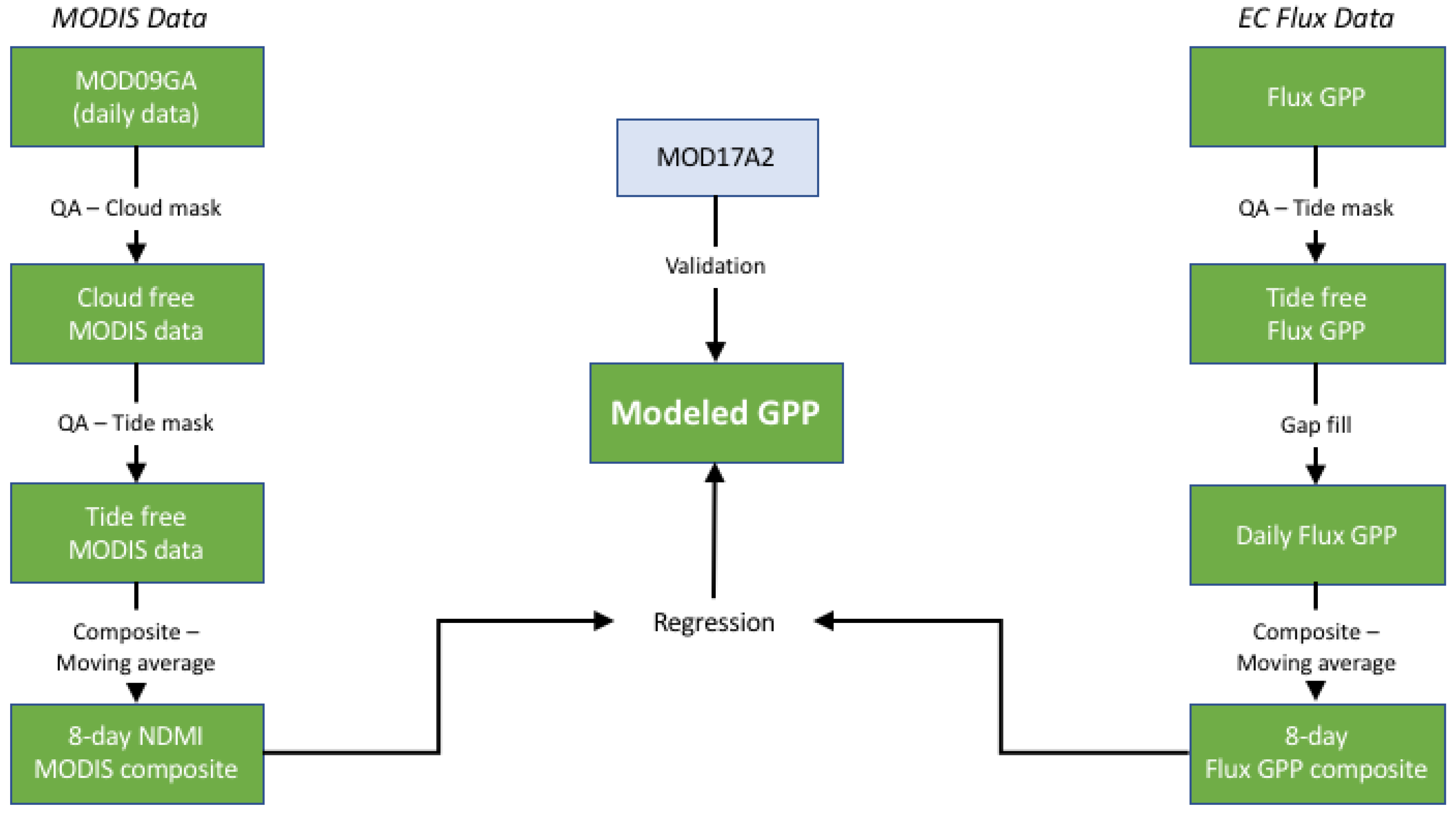
2.2.5. MODIS Data Preprocessing
2.3. Accounting for Tides in Flux and MODIS Data
2.3.1. Creating a Tide-Free GPP Time Series from Flux Data
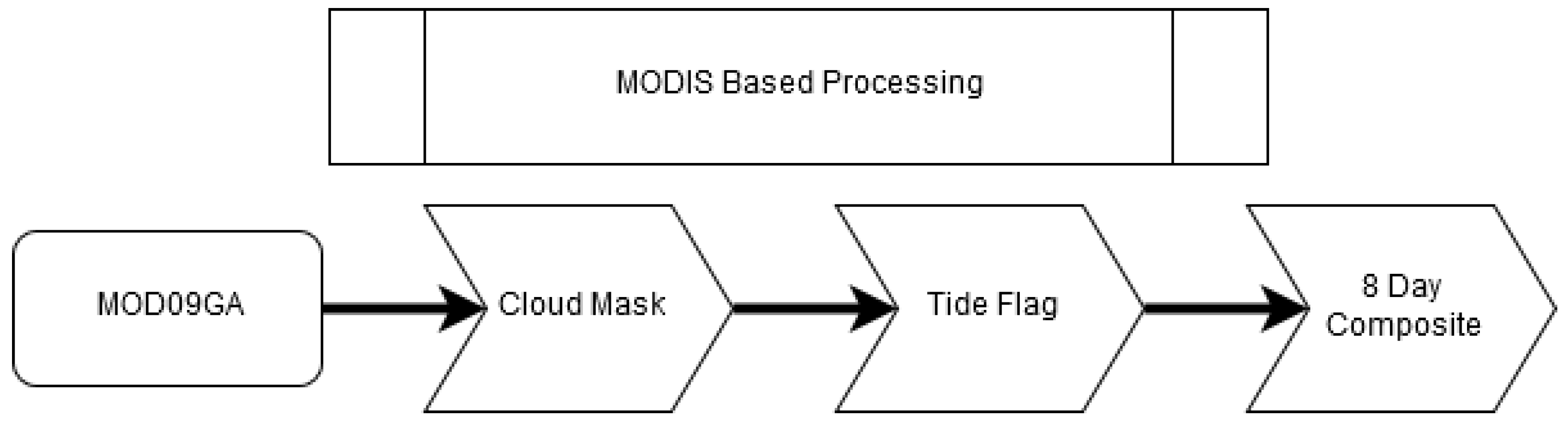
2.3.2. Creating Cloud-Free and Tide-Free MODIS VI Composites
2.4. Select the Best Vegetation Index as a Proxy for GPP
3. Results
3.1. Creating a Tide-Free GPP Time Series from Flux Data
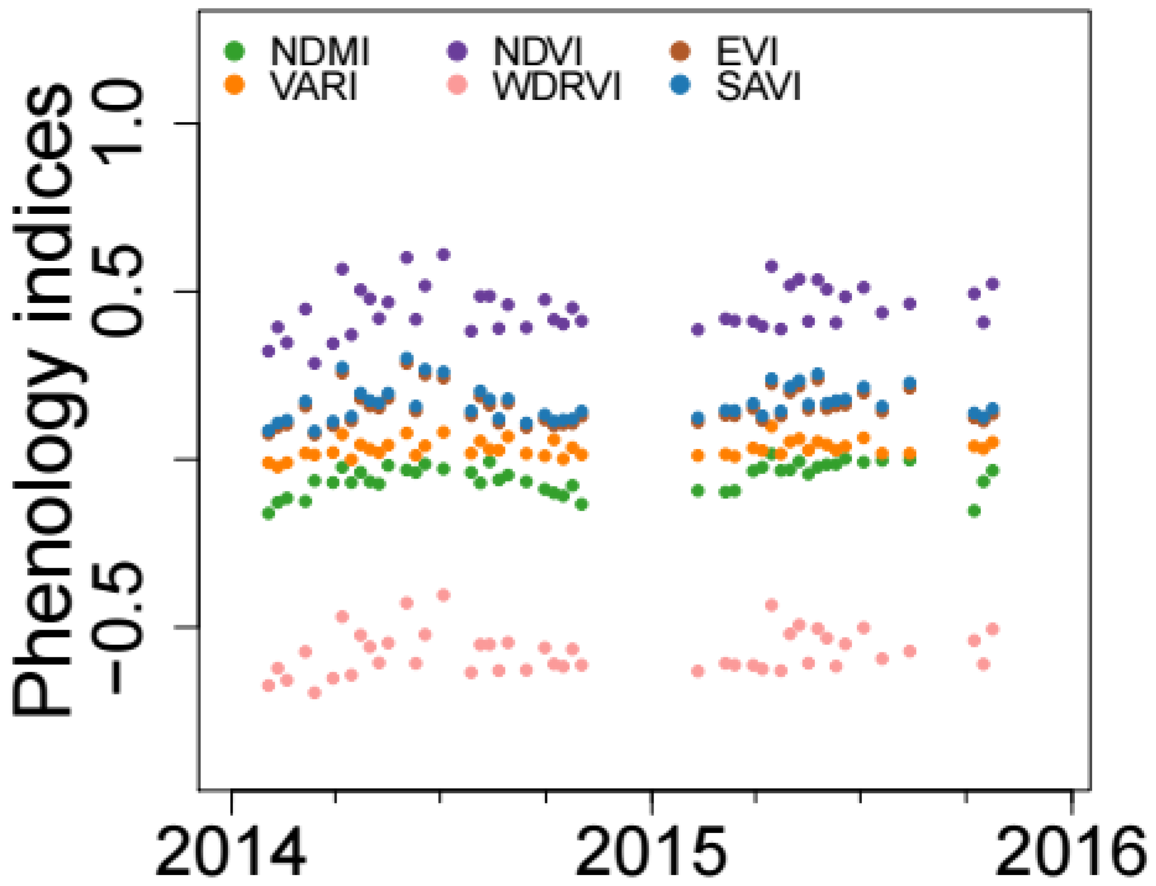
3.2. Creating Cloud-Free and Tide-Free MODIS VI Composites
3.3. Selection of the Best Vegetation Index as a Proxy for GPP from the Training Data
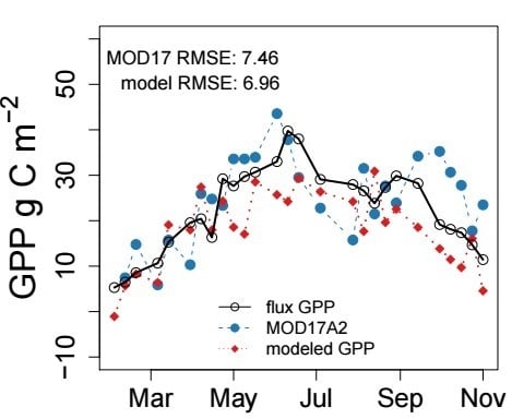
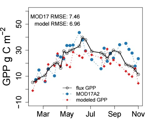
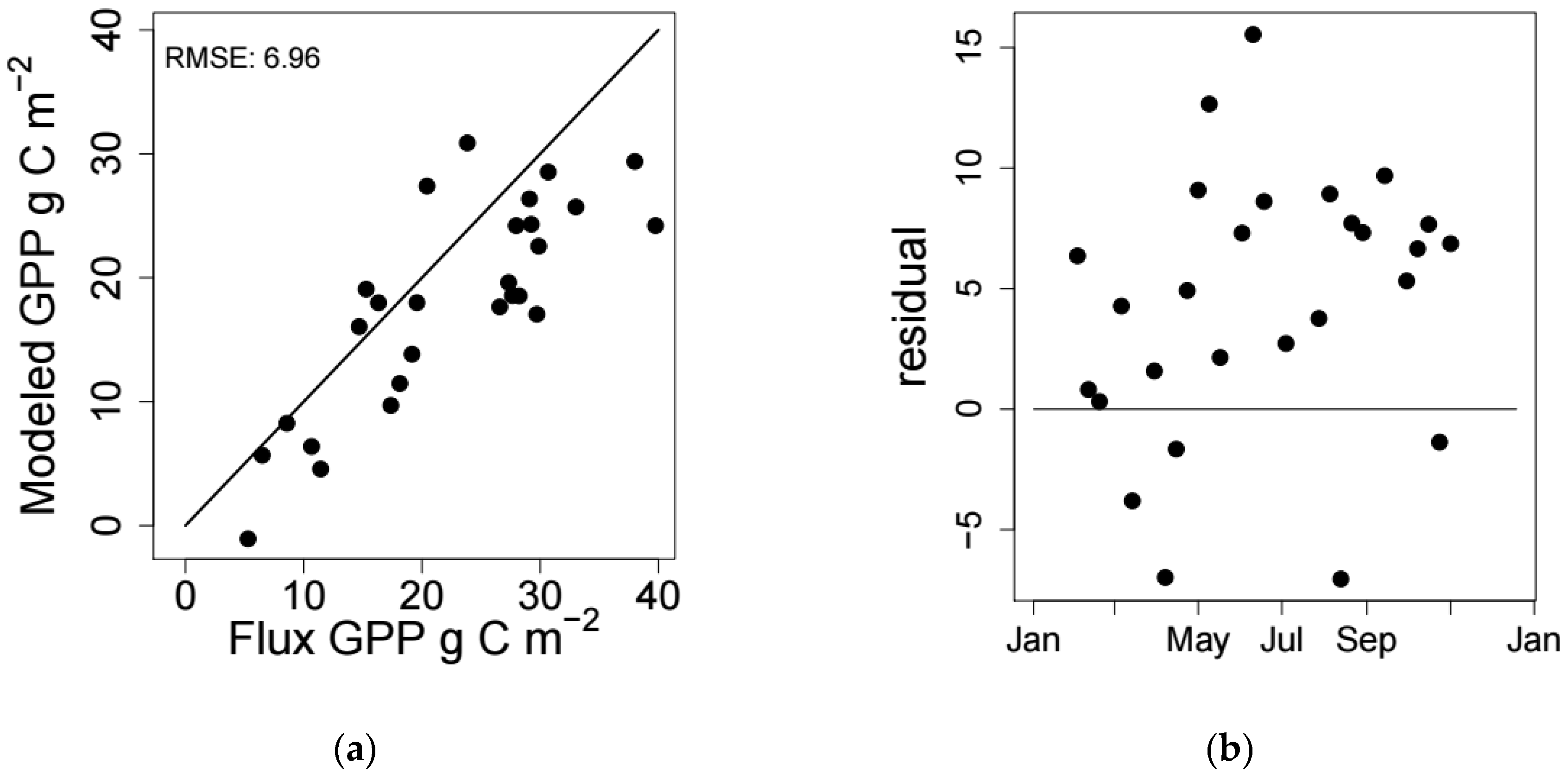
3.4. Modeling GPP from the Validation Data
4. Discussion
5. Conclusions
Author Contributions
Funding
Acknowledgments
Conflicts of Interest
References
- Barr, J.G.; Engel, V.; Fuentes, J.D.; Fuller, D.O.; Kwon, H. Modeling light use efficiency in a subtropical mangrove forest equipped with CO2 eddy covariance. Biogeosciences 2013, 10, 2145–2158. [Google Scholar] [CrossRef]
- Knox, S.H.; Windham-Myers, L.; Anderson, F.; Sturtevant, C.; Bergamaschi, B. Direct and Indirect Effects of Tides on Ecosystem-Scale CO2 Exchange in a Brackish Tidal Marsh in Northern California. J. Geophys. Res. Biogeosci. 2018, 123, 787–806. [Google Scholar] [CrossRef]
- Monteith, J.L. Solar Radiation and Productivity in Tropical Ecosystems. J. Appl. Ecol. 1972, 9, 747–766. [Google Scholar] [CrossRef]
- Oikawa, P.Y.; Jenerette, G.D.; Knox, S.H.; Sturtevant, C.; Verfaillie, J.; Dronova, I.; Poindexter, C.M.; Eichelmann, E.; Baldocchi, D.D. Evaluation of a hierarchy of models reveals importance of substrate limitation for predicting carbon dioxide and methane exchange in restored wetlands. J. Geophys. Res. Biogeosci. 2016, 122, 145–167. [Google Scholar] [CrossRef]
- Zhao, M.; Heinsch, F.A.; Nemani, R.R.; Running, S.W. Improvements of the MODIS terrestrial gross and net primary production global data set. Remote Sens. Environ. 2005, 95, 164–176. [Google Scholar] [CrossRef]
- Kirwan, M.L.; Megonigal, J.P. Tidal wetland stability in the face of human impacts and sea-level rise. Nature 2013, 504, 53–60. [Google Scholar] [CrossRef] [PubMed]
- Mcleod, E.; Chmura, G.L.; Bouillon, S.; Salm, R.; Björk, M.; Duarte, C.M.; Lovelock, C.E.; Schlesinger, W.H.; Silliman, B.R. A blueprint for blue carbon: Toward an improved understanding of the role of vegetated coastal habitats in sequestering CO2. Front. Ecol. Environ. 2011, 9, 552–560. [Google Scholar] [CrossRef] [Green Version]
- Ghosh, S.; Mishra, D. Analyzing the Long-Term Phenological Trends of Salt Marsh Ecosystem across Coastal LOUISIANA. Remote Sens. 2017, 9, 1340. [Google Scholar] [CrossRef]
- Mishra, D.; Ghosh, S. Using moderate resolution satellite sensors for monitoring the biophysical parameters and phenology of tidal wetlands. In Remote Sensing of Wetlands: Applications and Advances; Tiner, R.W., Lang, M.W., Klemas, V.V., Eds.; CRC Press: Boca Raton, FL, USA, 2015; pp. 283–314. ISBN 978-1-4822-3738-2. [Google Scholar]
- Chasmer, L.; Barr, A.; Hopkinson, C.; McCaughey, H.; Treitz, P.; Black, A.; Shashkov, A. Scaling and assessment of GPP from MODIS using a combination of airborne lidar and eddy covariance measurements over jack pine forests. Remote Sens. Environ. 2009, 113, 82–93. [Google Scholar] [CrossRef]
- Coops, N.C.; Black, T.A.; Jassal, R.S.; Trofymow, J.A.; Morgenstern, K. Comparison of MODIS, eddy covariance determined and physiologically modelled gross primary production (GPP) in a Douglas-fir forest stand. Remote Sens. Environ. 2007, 3, 385–401. [Google Scholar] [CrossRef]
- Kearney, M.S.; Stutzer, D.; Turpie, K.; Stevenson, J.C. The Effects of Tidal Inundation on the Reflectance Characteristics of Coastal Marsh Vegetation. J. Coast. Res. 2009, 25, 1177–1186. [Google Scholar] [CrossRef]
- Turpie, K.R. Explaining the Spectral Red-Edge Features of Inundated Marsh Vegetation. J. Coast. Res. 2013, 290, 1111–1117. [Google Scholar] [CrossRef]
- Ghosh, S.; Mishra, D.R.; Gitelson, A.A. Long-term monitoring of biophysical characteristics of tidal wetlands in the northern Gulf of Mexico—A methodological approach using MODIS. Remote Sens. Environ. 2016, 173, 39–58. [Google Scholar] [CrossRef]
- Moffett, K.B.; Wolf, A.; Berry, J.A.; Gorelick, S.M. Salt marsh–atmosphere exchange of energy, water vapor, and carbon dioxide: Effects of tidal flooding and biophysical controls. Water Resour. Res. 2010, 46. [Google Scholar] [CrossRef]
- Sims, D.; Rahman, A.; Cordova, V.; Elmasri, B.; Baldocchi, D.; Bolstad, P.; Flanagan, L.; Goldstein, A.; Hollinger, D.; Misson, L. A new model of gross primary productivity for North American ecosystems based solely on the enhanced vegetation index and land surface temperature from MODIS. Remote Sens. Environ. 2008, 112, 1633–1646. [Google Scholar] [CrossRef]
- Running, S.W.; Zhao, M. Daily GPP and Annual NPP (MOD17A2/A3) Products NASA Earth Observing System MODIS Land Algorithm; Version 3.0 for Collection 6; NASA: Greenbelt, MD, USA, 2015.
- Forbrich, I.; Giblin, A.E. Marsh-atmosphere CO2 exchange in a New England salt marsh. J. Geophys. Res. Biogeosci. 2015, 120, 1825–1838. [Google Scholar] [CrossRef]
- Sims, D.A.; Rahman, A.F.; Cordova, V.D.; El-Masri, B.Z.; Baldocchi, D.D.; Flanagan, L.B.; Goldstein, A.H.; Hollinger, D.Y.; Misson, L.; Monson, R.K.; et al. On the use of MODIS EVI to assess gross primary productivity of North American ecosystems. J. Geophys. Res. Biogeosci. 2006, 111. [Google Scholar] [CrossRef] [Green Version]
- Wu, C.; Niu, Z.; Gao, S. Gross primary production estimation from MODIS data with vegetation index and photosynthetically active radiation in maize. J. Geophys. Res. 2010, 115. [Google Scholar] [CrossRef] [Green Version]
- Gitelson, A.A.; Viña, A.; Verma, S.B.; Rundquist, D.C.; Arkebauer, T.J.; Keydan, G.; Leavitt, B.; Ciganda, V.; Burba, G.G.; Suyker, A.E. Relationship between gross primary production and chlorophyll content in crops: Implications for the synoptic monitoring of vegetation productivity. J. Geophys. Res. 2006, 111. [Google Scholar] [CrossRef] [Green Version]
- Inoue, Y.; Penuelas, J.; Miyata, A.; Mano, M. Normalized difference spectral indices for estimating photosynthetic efficiency and capacity at a canopy scale derived from hyperspectral and CO2 flux measurements in rice. Remote Sens. Environ. 2008, 112, 156–172. [Google Scholar] [CrossRef]
- Wu, C.; Niu, Z.; Tang, Q.; Huang, W.; Rivard, B.; Feng, J. Remote estimation of gross primary production in wheat using chlorophyll-related vegetation indices. Agric. For. Meteorol. 2009, 149, 1015–1021. [Google Scholar] [CrossRef]
- O’Connell, J.L.; Mishra, D.R.; Cotten, D.L.; Wang, L.; Alber, M. The Tidal Marsh Inundation Index (TMII): An inundation filter to flag flooded pixels and improve MODIS tidal marsh vegetation time-series analysis. Remote Sens. Environ. 2017, 201, 34–46. [Google Scholar] [CrossRef]
- Ge, Z.-M.; Guo, H.-Q.; Zhao, B.; Zhang, C.; Peltola, H.; Zhang, L.-Q.; Ge, Z.-M.; Guo, H.-Q.; Zhao, B.; Zhang, C.; et al. Spatiotemporal patterns of the gross primary production in the salt marshes with rapid community change: A coupled modeling approach. Ecol. Model. 2016, 321, 110–120. [Google Scholar] [CrossRef]
- Yan, Y.-E.; Guo, H.-Q.; Gao, Y.; Zhao, B.; Chen, J.-Q.; Li, B.; Chen, J.-K. Variations of net ecosystem CO2 exchange in a tidal inundated wetland: Coupling MODIS and tower-based fluxes. J. Geophys. Res. Atmos. 2010, 115. [Google Scholar] [CrossRef]
- Vickers, D.; Mahrt, L. Quality Control and Flux Sampling Problems for Tower and Aircraft Data. J. Atmos. Ocean. Technol. 1997, 14, 512–526. [Google Scholar] [CrossRef] [Green Version]
- Wilczak, J.M.; Oncley, S.P.; Stage, S.A. Sonic anemometer tilt correction algorithms. Bound.-Layer Meteorol. 2001, 99, 127–150. [Google Scholar] [CrossRef]
- Webb, E.K.; Pearman, G.I.; Leuning, R. Correction of flux measurements for density effects due to heat and water vapour transfer. Q. J. R. Meteorol. Soc. 1980, 106, 85–100. [Google Scholar] [CrossRef]
- Papale, D.; Reichstein, M.; Aubinet, M.; Canfora, E.; Bernhofer, C.; Kutsch, W.; Longdoz, B.; Rambal, S.; Valentini, R.; Vesala, T.; et al. Towards a standardized processing of Net Ecosystem Exchange measured with eddy covariance technique: Algorithms and uncertainty estimation. Biogeosciences 2006, 3, 571–583. [Google Scholar] [CrossRef]
- Falge, E.; Baldocchi, D.; Olson, R.; Anthoni, P.; Aubinet, M.; Bernhofer, C.; Burba, G.; Ceulemans, R.; Clement, R.; Dolman, H.; et al. Gap filling strategies for defensible annual sums of net ecosystem exchange. Agric. For. Meteorol. 2001, 107, 43–69. [Google Scholar] [CrossRef] [Green Version]
- Lloyd, J.; Taylor, J.A. On the Temperature Dependence of Soil Respiration. Funct. Ecol. 1994, 8, 315–323. [Google Scholar] [CrossRef]
- Reichstein, M.; Falge, E.; Baldocchi, D.; Papale, D.; Aubinet, M.; Berbigier, P.; Bernhofer, C.; Buchmann, N.; Gilmanov, T.; Granier, A.; et al. On the separation of net ecosystem exchange into assimilation and ecosystem respiration: Review and improved algorithm. Glob. Chang. Biol. 2005, 11, 1424–1439. [Google Scholar] [CrossRef]
- O’Connell, J.L.; Alber, M. A smart classifier for extracting environmental data from digital image time-series: Applications for PhenoCam data in a tidal salt marsh. Environ. Model. Softw. 2016, 84, 134–139. [Google Scholar] [CrossRef] [Green Version]
- Huete, A.; Didan, K.; Miura, T.; Rodriguez, E.P.; Gao, X.; Ferreira, L.G. Overview of the radiometric and biophysical performance of the MODIS vegetation indices. Remote Sens. Environ. 2002, 83, 195–213. [Google Scholar] [CrossRef]
- Balzarolo, M.; Vicca, S.; Nguy-Robertson, A.L.; Bonal, D.; Elbers, J.A.; Fu, Y.H.; Gruenwald, T.; Horemans, J.A.; Papale, D.; Penuelas, J.; et al. Matching the phenology of Net Ecosystem Exchange and vegetation indices estimated with MODIS and FLUXNET in-situ observations. Remote Sens. Environ. 2016, 174, 290–300. [Google Scholar] [CrossRef] [Green Version]
- Waring, R.H.; Coops, N.C.; Fan, W.; Nightingale, J.M. MODIS enhanced vegetation index predicts tree species richness across forested ecoregions in the contiguous USA. Remote Sens. Environ. 2006, 103, 218–226. [Google Scholar] [CrossRef]
- Rouse, J.W.; Haas, R.H.; Schell, J.A.; Deering, D.W. Monitoring vegetation systems in the Great Plains with ERTS. In NASA Goddard Space Flight Center 3d ERTS-1 Symp.; NASA: Greenbelt, MD, USA, 1974; Volume 1, Section A; pp. 309–317. [Google Scholar]
- Huete, A.R. A soil-adjusted vegetation index (SAVI). Remote Sens. Environ. 1988, 25, 295–309. [Google Scholar] [CrossRef]
- Gao, B.-C. NDWI—A normalized difference water index for remote sensing of vegetation liquid water from space. Remote Sens. Environ. 1996, 58, 257–266. [Google Scholar] [CrossRef]
- Gitelson, A.A.; Stark, R.; Grits, U.; Rundquist, D.; Kaufman, Y.; Derry, D. Vegetation and soil lines in visible spectral space: A concept and technique for remote estimation of vegetation fraction. Int. J. Remote Sens. 2002, 23, 2537–2562. [Google Scholar] [CrossRef]
- Gitelson, A.A. Wide dynamic range vegetation index for remote quantification of biophysical characteristics of vegetation. J. Plant Physiol. 2004, 161, 165–173. [Google Scholar] [CrossRef] [PubMed]
- Thenkabail, P.S.; Mariotto, I.; Gumma, M.K.; Middleton, E.M.; Landis, D.R.; Huemmrich, K.F. Selection of hyperspectral narrowbands (HNBs) and composition of hyperspectral twoband vegetation indices (HVIs) for biophysical characterization and discrimination of crop types using field reflectance and Hyperion/EO-1 data. IEEE J. Sel. Top. Appl. Earth Obs. Remote Sens. 2013, 6, 13. [Google Scholar] [CrossRef]
- Hessini, K.; Ghandour, M.; Albouchi, A.; Soltani, A.; Werner, K.H.; Abdelly, C. Biomass production, photosynthesis, and leaf water relations of Spartina alterniflora under moderate water stress. J. Plant Res. 2008, 121, 311–318. [Google Scholar] [CrossRef] [PubMed]
- Xiao, X.; Hollinger, D.; Aber, J.; Goltz, M.; Davidson, E.A.; Zhang, Q.; Iii, B.M. Satellite-based modeling of gross primary production in an evergreen needleleaf forest. Remote Sens. Environ. 2004, 89, 519–534. [Google Scholar] [CrossRef]
- Xiao, X.; Zhang, Q.; Braswell, B.; Urbanski, S.; Boles, S.; Wofsy, S.; Moore, B.; Ojima, D. Modeling gross primary production of temperate deciduous broadleaf forest using satellite images and climate data. Remote Sens. Environ. 2004, 91, 256–270. [Google Scholar] [CrossRef]
- Running, S.W.; Thornton, P.E.; Nemani, R.; Glassy, J.M. Global Terrestrial Gross and Net Primary Productivity from the Earth Observing System. In Methods in Ecosystem Science; Springer: New York, NY, USA, 2000; pp. 44–57. ISBN 978-0-387-98743-9. [Google Scholar]
- Running, S.W.; Nemani, R.R.; Heinsch, F.A.; Zhao, M.; Reeves, M.; Hashimoto, H. A Continuous Satellite-Derived Measure of Global Terrestrial Primary Production. Bioscience 2004, 54, 547–560. [Google Scholar] [CrossRef]
- McCallum, I.; Franklin, O.; Moltchanova, E.; Merbold, L.; Schmullius, C.; Shvidenko, A.; Schepaschenko, D.; Fritz, S. Improved light and temperature responses for light-use-efficiency-based GPP models. Biogeosciences 2013, 10, 6577–6590. [Google Scholar] [CrossRef] [Green Version]
- Wei, S.; Yi, C.; Fang, W.; Hendrey, G. A global study of GPP focusing on light-use efficiency in a random forest regression model. Ecosphere 2017, 8, e01724. [Google Scholar] [CrossRef]


| Modeling (2015) | Validation (2014) | |
|---|---|---|
| Daily surface reflectance | 360 | 358 |
| Cloud-free, low view zenith | 52 | 67 |
| Cloud and tide free | 44 | 61 |
| 8 day composite | 20 | 27 |
| Index | R2 |
|---|---|
| NDVI | 0.04 |
| SAVI | 0.38 |
| NDMI | 0.46 |
| VARI | 0.05 |
| EVI | 0.38 |
| WDRVI | 0.03 |
© 2018 by the authors. Licensee MDPI, Basel, Switzerland. This article is an open access article distributed under the terms and conditions of the Creative Commons Attribution (CC BY) license (http://creativecommons.org/licenses/by/4.0/).
Share and Cite
Tao, J.; Mishra, D.R.; Cotten, D.L.; O’Connell, J.; Leclerc, M.; Nahrawi, H.B.; Zhang, G.; Pahari, R. A Comparison between the MODIS Product (MOD17A2) and a Tide-Robust Empirical GPP Model Evaluated in a Georgia Wetland. Remote Sens. 2018, 10, 1831. https://0-doi-org.brum.beds.ac.uk/10.3390/rs10111831
Tao J, Mishra DR, Cotten DL, O’Connell J, Leclerc M, Nahrawi HB, Zhang G, Pahari R. A Comparison between the MODIS Product (MOD17A2) and a Tide-Robust Empirical GPP Model Evaluated in a Georgia Wetland. Remote Sensing. 2018; 10(11):1831. https://0-doi-org.brum.beds.ac.uk/10.3390/rs10111831
Chicago/Turabian StyleTao, Jianbin, Deepak R Mishra, David L. Cotten, Jessica O’Connell, Monique Leclerc, Hafsah Binti Nahrawi, Gengsheng Zhang, and Roshani Pahari. 2018. "A Comparison between the MODIS Product (MOD17A2) and a Tide-Robust Empirical GPP Model Evaluated in a Georgia Wetland" Remote Sensing 10, no. 11: 1831. https://0-doi-org.brum.beds.ac.uk/10.3390/rs10111831