Article

Freshwater Fish Habitat Complexity Mapping Using Above and Underwater Structure-From-Motion Photogrammetry

1
Department of Geography, Applied Remote Sensing Lab, McGill University, Montreal, QC H3A 0B9, Canada
2
Laboratório de Ictiologia de Altamira, Universidade Federal do Pará, Altamira, PA 68372-040, Brazil
3
Flight Research Lab, National Research Council Canada, Ottawa, ON K1A 0R6, Canada
*
Author to whom correspondence should be addressed.
Remote Sens. 2018, 10(12), 1912; https://0-doi-org.brum.beds.ac.uk/10.3390/rs10121912
Submission received: 28 September 2018 / Revised: 20 November 2018 / Accepted: 28 November 2018 / Published: 29 November 2018
(This article belongs to the Special Issue Drone Remote Sensing)

Abstract

:
Substrate complexity is strongly related to biodiversity in aquatic habitats. We illustrate a novel framework, based on Structure-from-Motion photogrammetry (SfM) and Multi-View Stereo (MVS) photogrammetry, to quantify habitat complexity in freshwater ecosystems from Unmanned Aerial Vehicle (UAV) and underwater photography. We analysed sites in the Xingu river basin, Brazil, to reconstruct the 3D structure of the substrate and identify and map habitat classes important for maintaining fish assemblage biodiversity. From the digital models we calculated habitat complexity metrics including rugosity, slope and 3D fractal dimension. The UAV based SfM-MVS products were generated at a ground sampling distance (GSD) of 1.20–2.38 cm while the underwater photography produced a GSD of 1 mm. Our results show how these products provide spatially explicit complexity metrics, which are more comprehensive than conventional arbitrary cross sections. Shallow neural network classification of SfM-MVS products of substrate exposed in the dry season resulted in high accuracies across classes. UAV and underwater SfM-MVS is robust for quantifying freshwater habitat classes and complexity and should be chosen whenever possible over conventional methods (e.g., chain-and-tape) because of the repeatability, scalability and multi-dimensional nature of the products. The SfM-MVS products can be used to identify high priority freshwater sectors for conservation, species occurrences and diversity studies to provide a broader indication for overall fish species diversity and provide repeatability for monitoring change over time.

Graphical Abstract

1. Introduction

In community ecology there are several theories to explain the distribution of species across environmental gradients. For instance, niche theory describes an n-dimensional hyper-volume of conditions and resources in which populations have a positive growth rate [1]. To understand species distributions along environmental gradients using niche theory is challenging however, because a niche is partitioned into conditions (e.g., habitat characteristics) and resources (e.g., food availability) and results will vary according to the methods used to quantify the habitat characteristics [2].
Remote sensing provides opportunities to characterize aquatic habitat structures with repeatability and robust quantitative metrics. At large spatial scales, freely available satellite imagery has been used to map river networks at scales from individual rivers or basins to the entire globe [3,4]. However, at small scales, satellite imagery with fine spatial resolution (<5 m) is expensive and not always available for specific sites on the optimal date(s) due to cloud cover (especially in the tropics) or satellite revisit times. The recent developments in unmanned aerial vehicle (UAV) platforms for ecological applications [5,6,7] are revolutionizing the way ecological variables can be mapped at the spatial and temporal scales needed for community ecology and environmental studies.
In terrestrial environments, UAV based photography [8,9,10] and Structure from Motion (SfM) with multi-view stereo (MVS) photogrammetry to produce 3D reconstructions of landscapes is increasingly popular [11,12]. In a strict sense our use of the term SfM refers to an analytical workflow that combines both SfM and MVS photogrammetry often followed by interpolation and in some cases textured mesh generation as described in Reference [13] but use SfM-MVS throughout for brevity. When correctly implemented, UAV SfM-MVS products have high spatial accuracy, even to within the error of differential GPS measurements [13,14,15,16,17]. The landscape reconstructions from SfM-MVS are also much higher spatial resolution (<1–5 cm) than conventional satellite imagery used to assess land cover change. Recently, SfM-MVS from underwater photography and videography has been used to model coral specimens [18], reefs [19,20,21,22,23] and vertical wall marine environments [24] with relatively high accuracies [21]. It has also been shown to be a powerful analytical approach for deep sea applications of terrain and object reconstruction [25]. In freshwater fluvial ecosystems, UAV SfM-MVS has been used to derive submerged digital elevation models and reach-scale morphology [26,27]. However, to the best of our knowledge, SfM-MVS (from UAV or underwater photography) has not yet been explored for freshwater fish habitat complexity characterization.
Biodiversity is strongly related to habitat structural complexity in both marine and freshwater environments [28,29,30,31,32,33,34]. While several definitions of habitat complexity have been used interchangeably with heterogeneity and diversity [35], in this study, we refer to habitat diversity as the variety of substrate types (e.g., sand, pebbles, boulders, bedrock) and heterogeneity as the magnitude of substrate diversity within a study site such as patches of sand interspersed with rocks versus homogenous sand. We further refer to complexity as the heterogeneity in the arrangement of substrate types within the habitat [36,37]. Metrics for quantifying aquatic habitat complexity and diversity include rugosity [32,38,39], spatial autocorrelation [40], fractal geometry [23,35,41], grain size [34], corrugation [42], current velocity [43], optical intensity [32], slope and aspect [44,45].
In freshwater ecology, most studies use either low-tech methods (e.g., chain-and-tape) or proxies (e.g., abundance of macrophytes, submerged vegetation) to infer habitat complexity [37,46,47,48,49]. The simple and subjective sampling methods (e.g., chain-and-tape) are time consuming, labour intensive and importantly, non-spatially extensive [23,50]. With the chain-and-tape method, a rope or chain is draped over the substrate profile and its length is measured and compared to the linear distance measured over the transect to produce a ‘substrate rugosity index’ (SRI) [51]. It is one of the most commonly used methods to quantify aquatic habitat complexity despite its well-known weaknesses [37,51]. For this reason, in marine environments, the SRI has been shown to be less accurate than digital 3D reconstructions of the habitat structures [18,23,50]. In freshwater ecosystems, distinguishing complexity and diversity among substrate profiles (a weakness of the SRI) is of fundamental importance to the aquatic biodiversity that inhabit only certain habitat types (e.g., large boulders vs. sand).
In this study, our goals are to illustrate the utility of SfM-MVS from UAV and underwater photography to quantify the habitat complexity in freshwater ecosystems and to map the area of habitat classes important for endemic and/or specialized ichthyofauna. Because SfM-MVS is still in early stages of adoption in the freshwater ecological communities [52], there is a lack of good practice guidelines (e.g., sensor, lens choice, resolution, lighting effects). Our discussion addresses these aspects as means to provide an initial set of recommendations for freshwater habitat SfM-MVS studies.

2. Materials and Methods
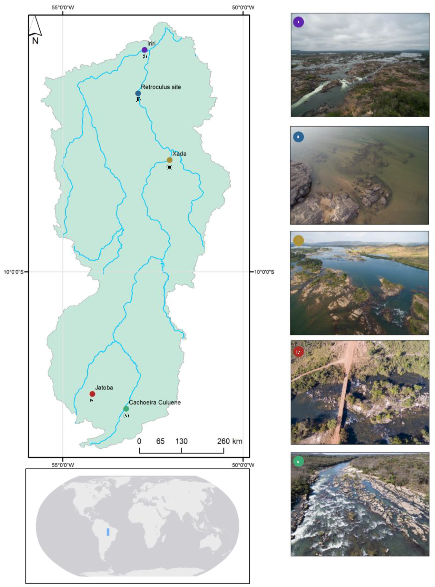
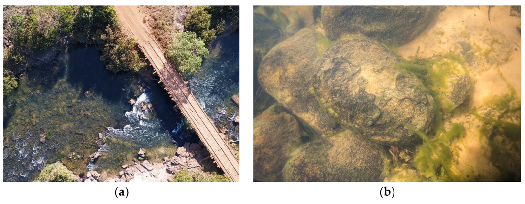
2.1. Study Area

Fieldwork was carried out at five sites in the Xingu river basin, Brazil. The Xingu is one of the primary tributaries of the Amazon River, contributing 5% of its annual freshwater discharge [53] (Figure 1). The river drains approximately 500,000 km2 of the Brazilian Shield [54]. It is oligotrophic with a low conductivity and high transparency [54] and is known for exceptionally high fish species richness and specialized taxa (450 fish species from 48 families are known, of which 60 species are endemic and 35 remain undescribed) [55].
Our primary study site is located on the Jatobá river, a north flowing tributary of the Xingu (Figure 1). At this location the water depth ranges from 15 cm to ~2.5 m in the dry season. The substrate is primarily comprised of gravel assemblages (2.5–15 cm grain size) and medium boulders (15–50 cm grain size) (Table 1). At least 17 fish species (14 genera) are known to inhabit this small section of the river (45 m long × 30 m wide) including characins (e.g., Astyanax anterior), cichlids (e.g., Geophagus agyrosticus), anostomids (e.g., Leporellus vittatus) and loricariids (Ancistrus sp.). The habitat is also representative of the types of substrate structure preferred by larger predatory benthopelagic species such as Hoplias aimara.
To evaluate the potential of SfM-MVS over a broader range of habitat diversity than what is present at the Jatobá site, we include four additional sites along the Xingu river and two of its main tributaries, the Iriri and Culuene rivers (Figure 1). The receded flood pulse from the wet season allowed for studying habitats at low water levels. During the dry season, large areas of substrate are exposed in areas covered (partially or completely) by fast flowing, deep and more turbid water during the rest of the year. (Figure 2).

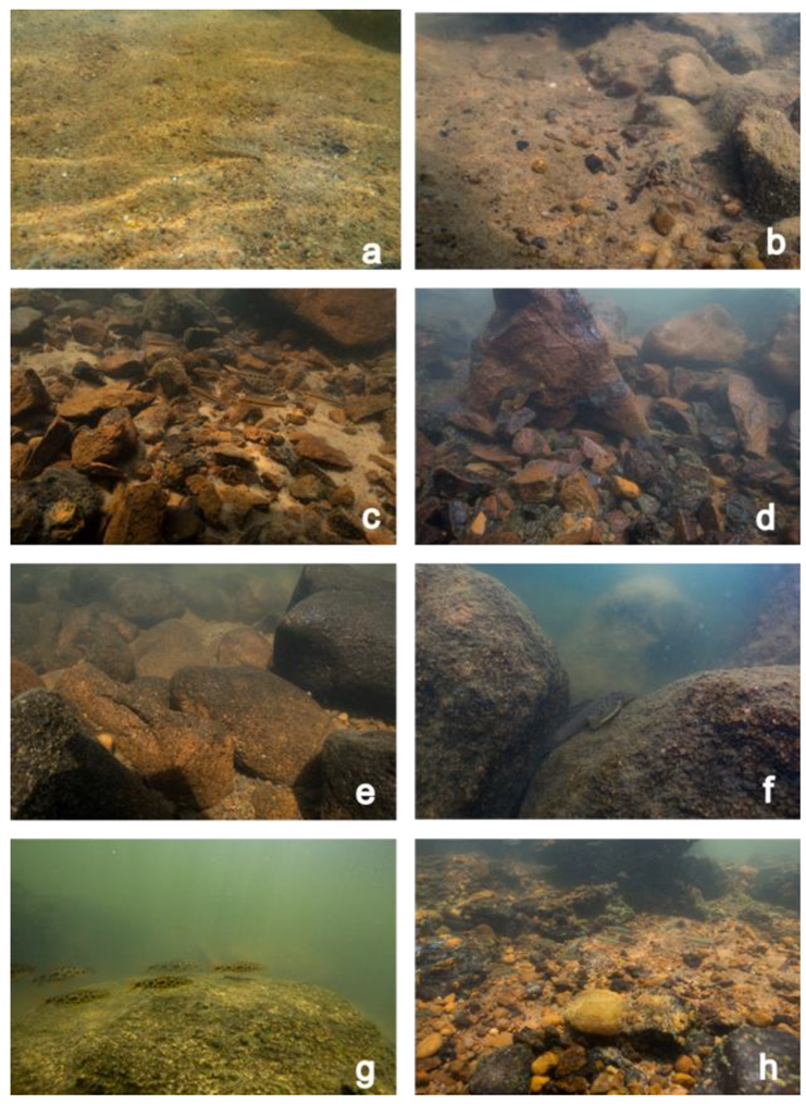
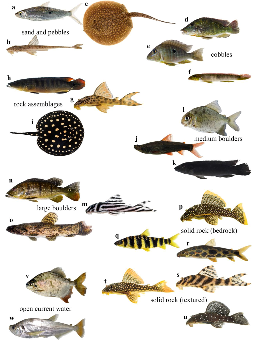
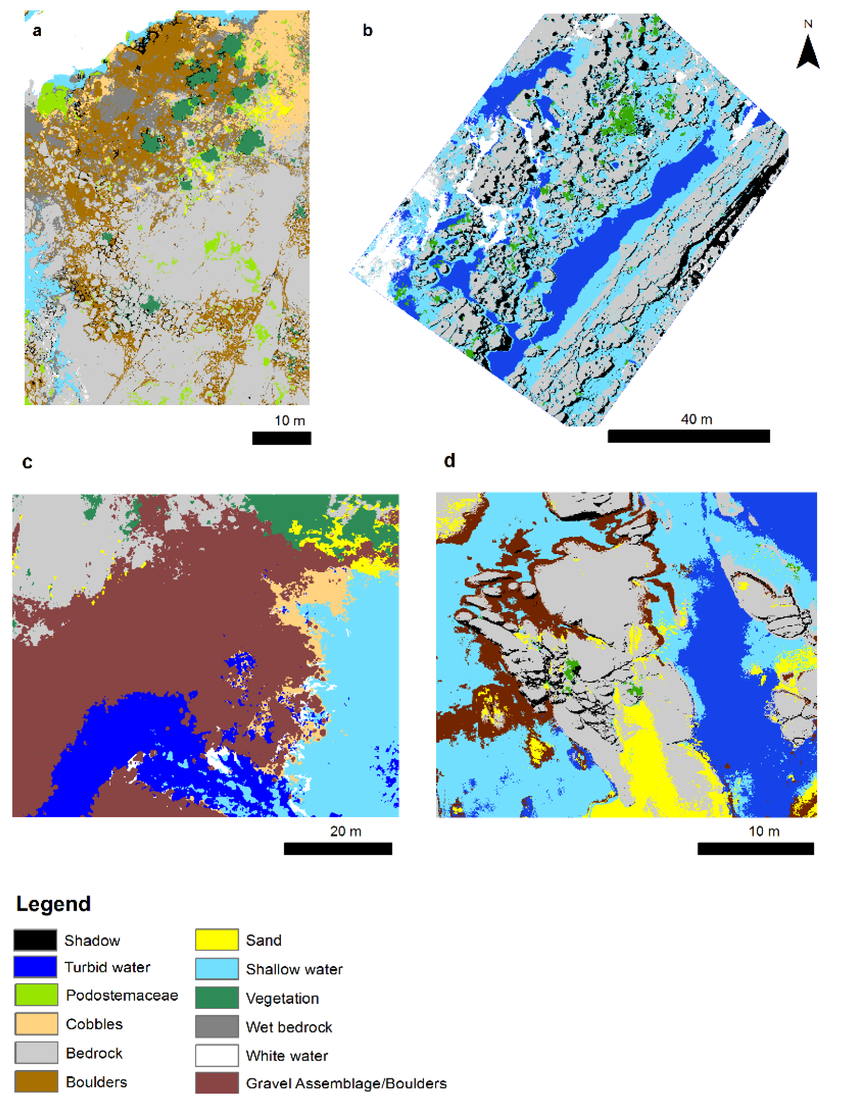
2.2. Habitat Class Descriptions

To examine the utility of the SfM-MVS for quantifying the habitat extent and complexity important to the fish assemblages of the Xingu, we define nine habitat classes considered essential for aquatic diversity based on over 2,000 hrs of personal underwater observation and as described by [56]. The heterogeneity of habitat classes is important because many species are preferentially associated with each (Figure 3 and Figure 4, Table 1). For example, the cichlid Crenicichla dandara prefers shadows of large rocks (medium and large boulder classes) where its dark coloration provides camouflage from its prey [57]. However, other than a few species that have obligate associations to a specific habitat class (e.g., Hypancistrus zebra to the large boulder class), there is overlap between some habitat classes where various species have been observed to occur. The grain size descriptions in Table 1 are based on the Wentworth scale with modifications to the ranges based on relevance to the fish species as observed in the field.

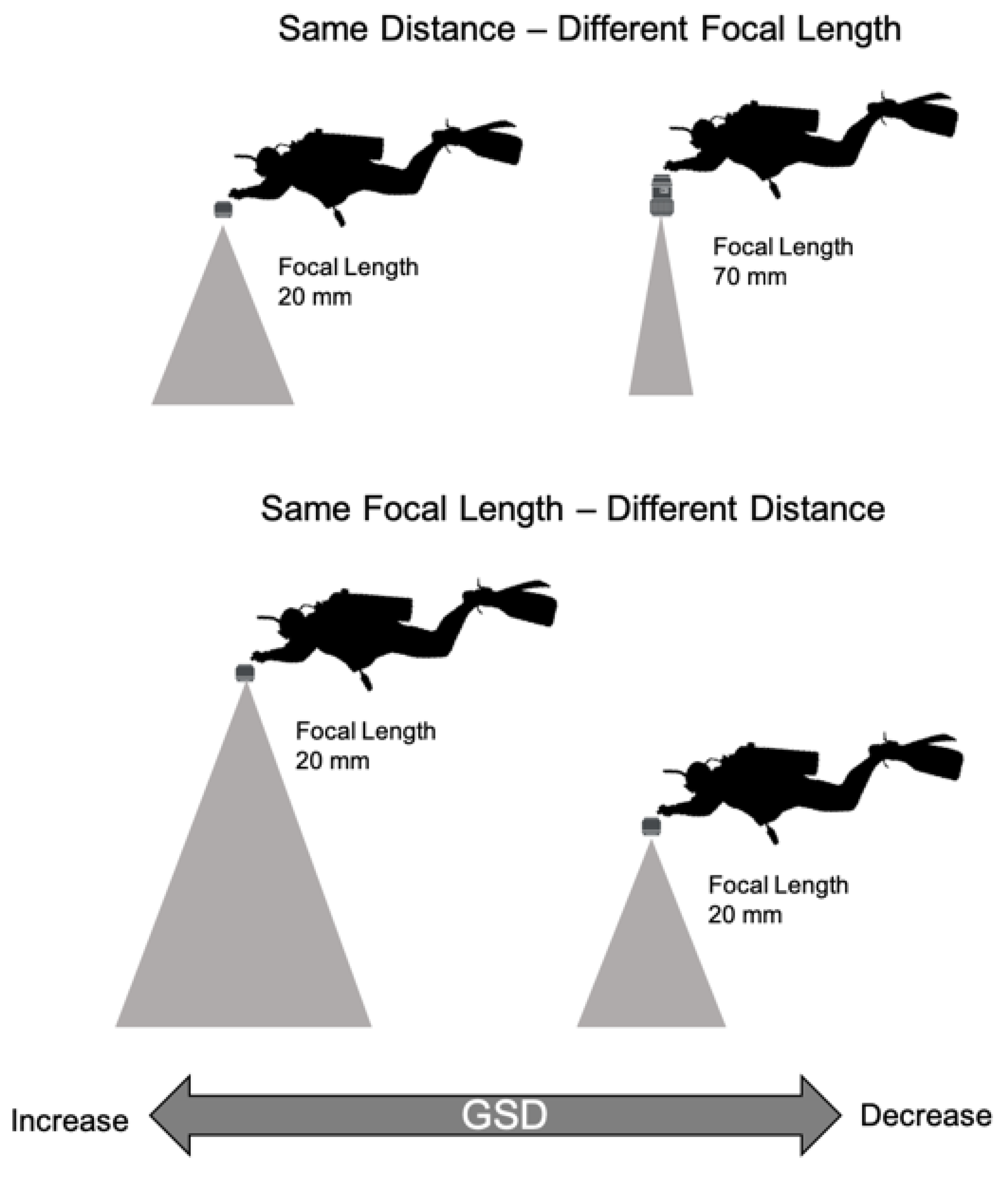
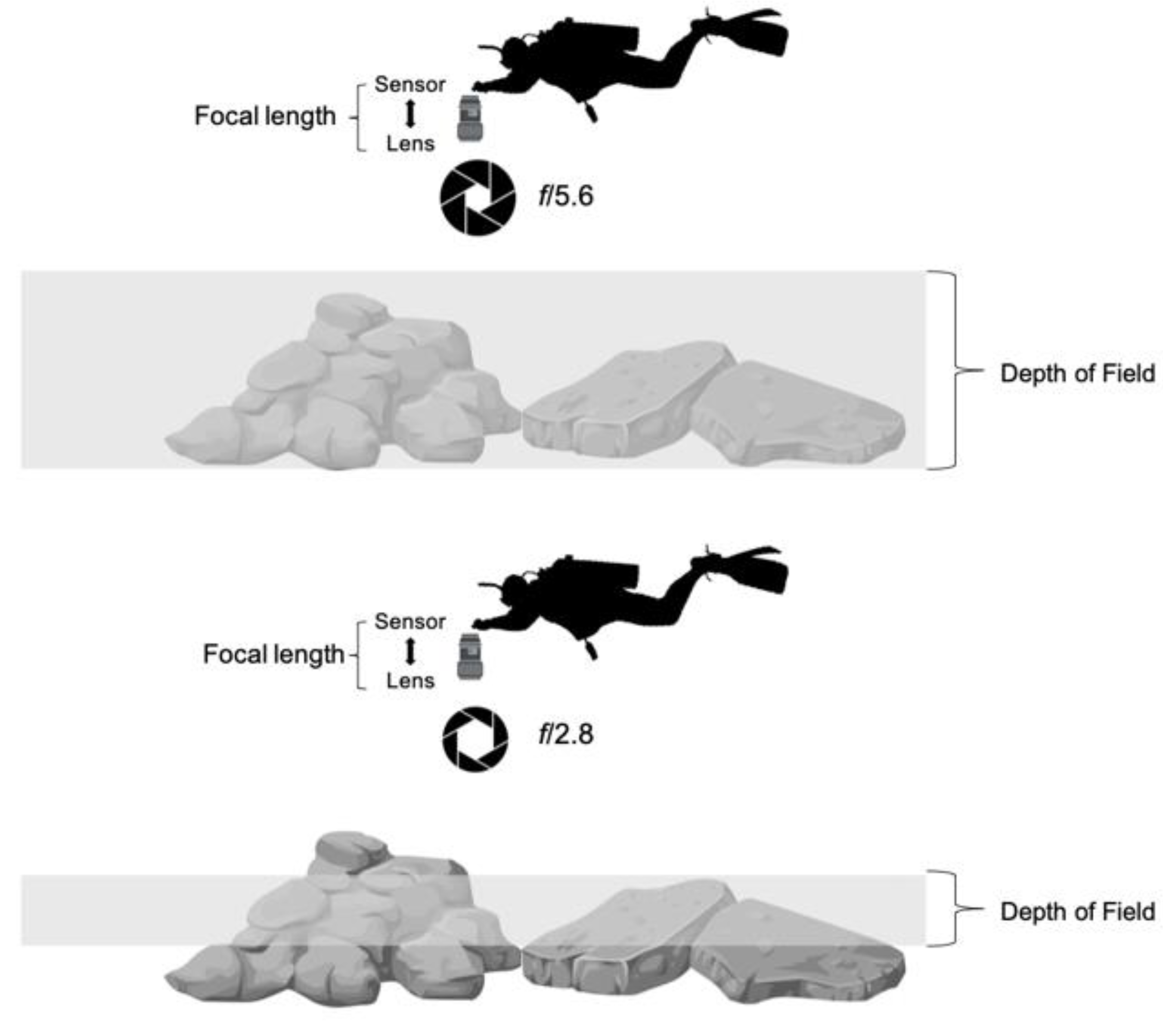
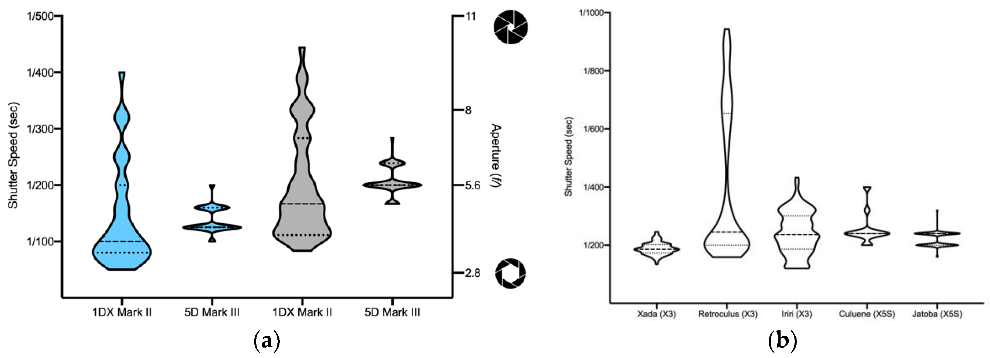
2.3. Unmanned Aerial Vehicle (UAV) and Underwater Photographs

Two models of UAVs were used (Table 2). The DJI Inspire 1 is a 2.9 kg 4-rotor UAV. It has an X3 FC350 12.4 MP camera and integrated 3-axis gimbal (±0.03°). The camera has a 1/2.3″ CMOS sensor, a fixed 20 mm lens with a 94° diagonal field of view and a linear rolling shutter producing an image size of 4000 × 3000 pixels. The DJI Inspire 2 is a 3.4 kg 4- rotor UAV. It was used with an X5S camera which has a micro 4/3 sensor, linear rolling shutter, integrated 3-axis gimbal (±0.01°) and a DJI MFT 15 mm/1.7 aspherical lens (72° diagonal field of view) producing an image size of 5280 × 3956 pixels (Figure 5a). Flights were conducted as two orthogonal grids (i.e., double grid pattern). All photographs included the geolocation of the centre of the frame and the altitude in the EXIF data. The unmodified geolocation is expected to have an absolute positional error up to 3 m. Because there were no GNSS active control stations within 100 km of the study sites and the limited time available at each site for data collection, no post processing correction was applied to the geolocations in the EXIF data, nor were any control points collected on site. The positional errors of non-post processed GPS positions were found to be of the same magnitude as the geolocation from the UAVs and therefore would not improve the overall absolute position of the UAV generated data.
Underwater photographs were collected at the Jatobá site with a Canon 5D Mark III DSLR with an EF 24–70 mm f/2.8L II USM lens set to 24 mm in autofocus mode (Figure 5b). This is a full-frame camera with a 36 × 24 mm CMOS sensor producing 22.3 MP effective pixels (5760 × 3840 pixels). The photographs were collected using a median aperture of f/5.6 with ISO 200 and saved in Canon RAW (.CR2) format. The camera was used with an Aquatica Housing and 8” dome port. Photographs were taken with the back of the housing at the surface of the water and the dome port as nadir as possible. A single grid pattern was used to acquire four rows of photographs with 71–72 frames per row (287 frames total) over a period of 30 min (one camera operator in snorkel gear). Overlap was visually estimated by the operator. The water depth in the study area was <1.8 m. Photographs were exported as full resolution TIFFs for analysis.

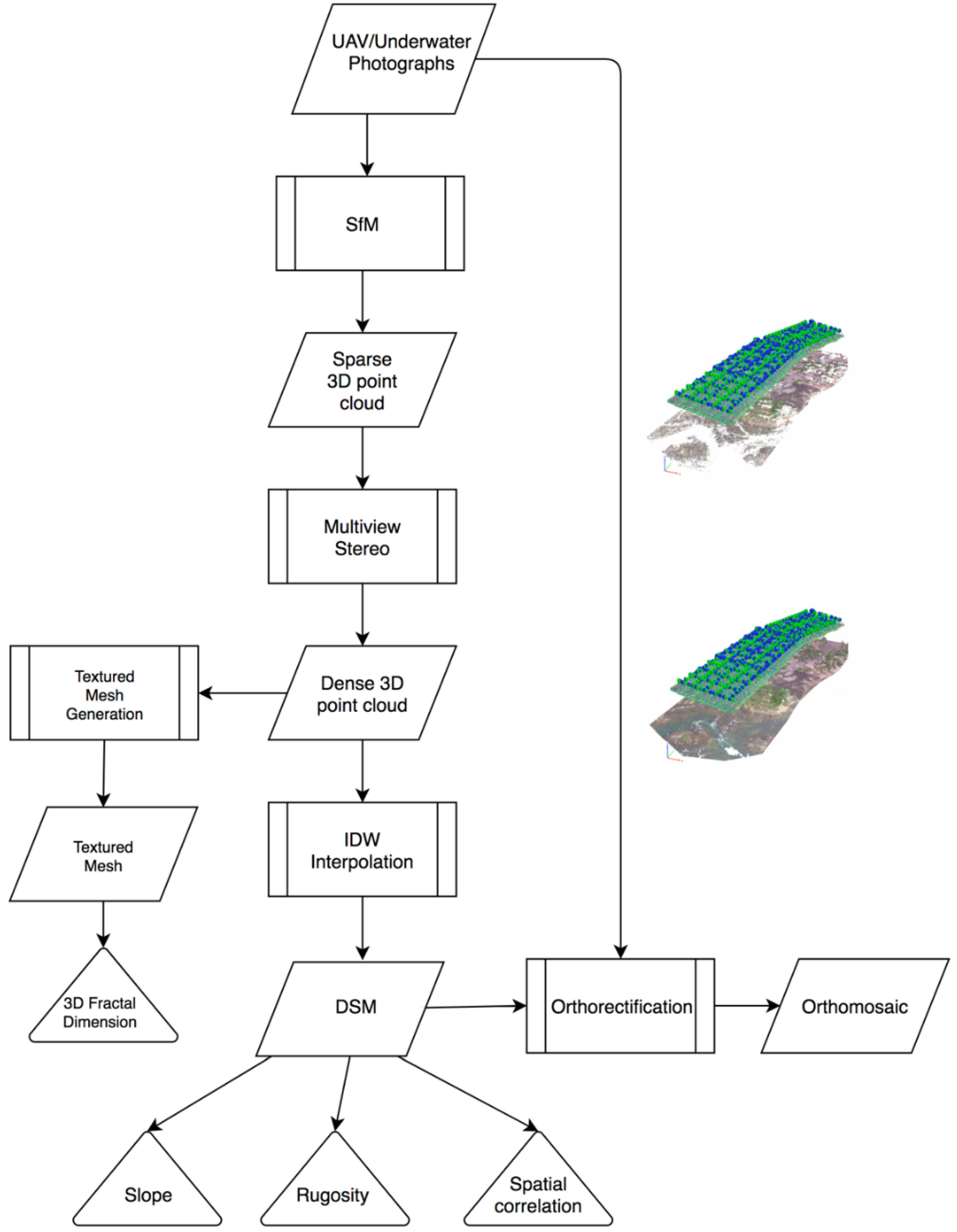
2.4. Structure from Motion (SfM)-Multi-View Stereo (MVS) Photogrammetry Products

SfM-MVS products consisting of an orthomosaic, dense 3D point cloud, triangular mesh and digital surface model (DSM) were generated from the UAV photographs with Pix4D Mapper Pro (Figure 6) [13,15,58] with ground sampling distances (GSD) ranging from 1.20–2.38 cm (Table 2). A refractive index submerged DSM correction was applied following [26,59,60] prior to the calculation of the habitat complexity metrics (Section 2.5). The SfM-MVS workflow was also used for the underwater photographs to create the same products with a GSD of 1 mm. No refractive index correction was applied to the DSM created from the underwater photographs. Pix4D utilizes a modification of the SIFT algorithm [61] where local gradients rather than sample intensities are used to create descriptors of each key point [62]. Following the generation of the initial 3D point cloud, a multi-view stereo photogrammetry algorithm is implemented to increase the density of the point cloud [63]. The raster DSM is generated through an inverse distance weighting interpolation of the dense 3D point cloud. The dense 3D point clouds were also converted to a textured mesh in Pix4D to facilitate the calculation of the fractal dimension [41].

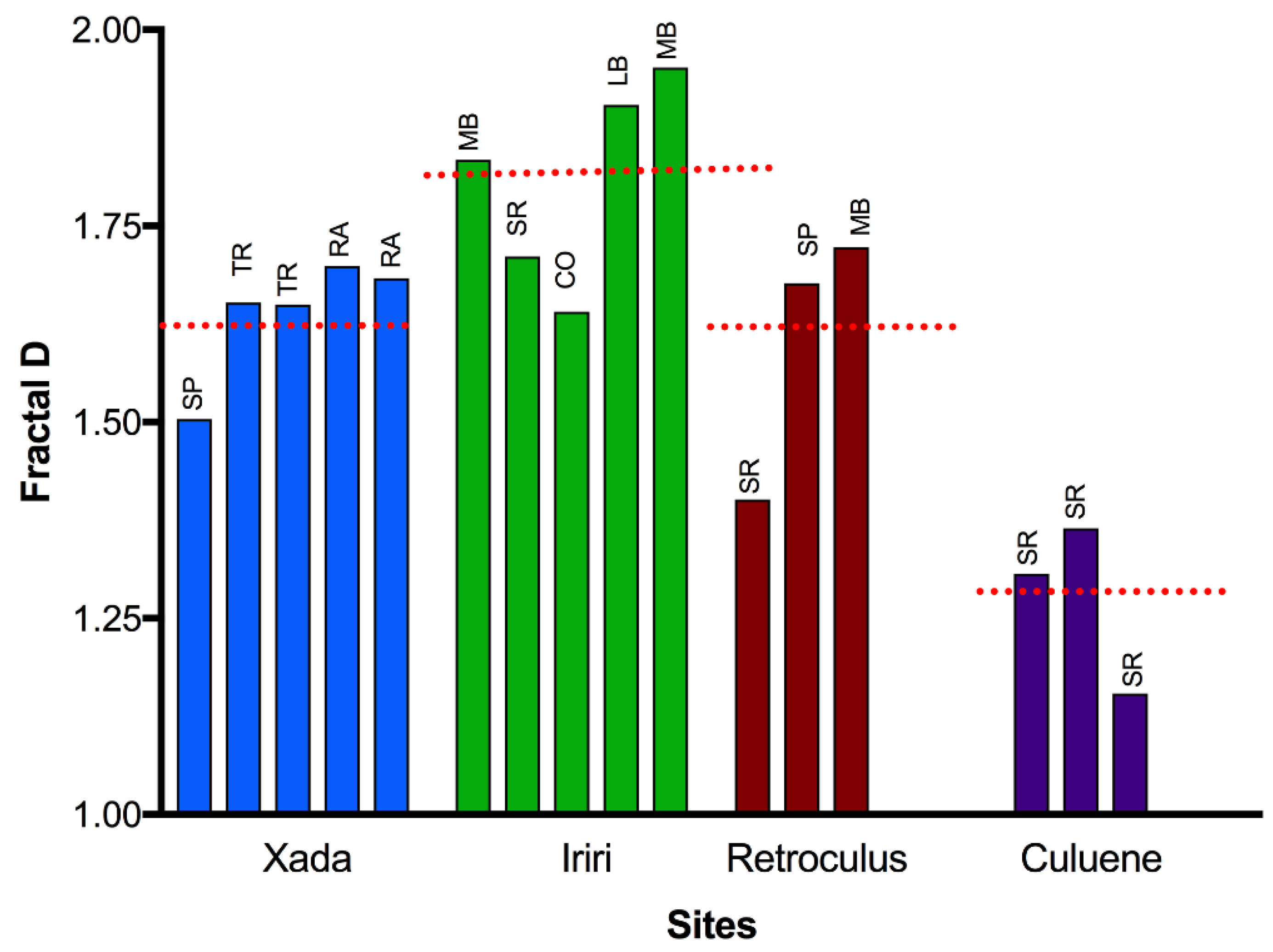
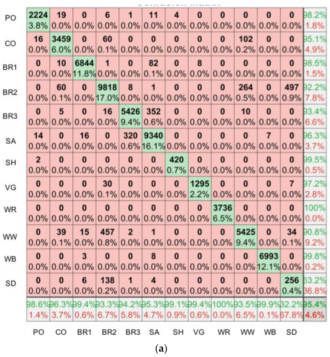
2.5. Habitat Complexity Metrics and Classification

The complexity metrics used here are indicators of the amount of available habitat and shelter for the benthic organisms and the amount of brood care and foraging area for mobile species. At the Jatobá site, from the submerged DSM, we calculated: (1) slope; (2) the autocorrelation of the surface topographic variation; and (3) the arc-chord ratio, a measure of rugosity expressed as the surface to planar area corrected for slope [45,64]. These metrics were calculated at a GSD of 1.2 cm (Table 2). From the underwater SfM-MVS the same metrics were calculated at the original GSD (1 mm) and at two coarser spatial scales (3 and 15 cm) arbitrarily chosen to represent the relevant habitat complexity for two common size classes of fishes found in the river. For comparison, from the underwater SfM-MVS DSM we calculated digital chain-and-tape SRI with a chain link size of 1 cm.
At the other four study sites (Table 2, Figure 1), from the textured mesh, we calculated the Minkowski–Bouligand fractal dimension as a measure of 3D complexity [41] for the habitat classes (Table 1, Figure 3) that were exposed by the low water level of the dry season. This metric has been used for shape quantification and complexity characterization of irregularly shaped organisms such as corals [41]. The fractal dimension, D, includes information from various spatial scales, where increasing values of D, from 0–3, indicate higher complexity (i.e., increasing roughness of shape) [41,65].
The exposed substrate from the Xada, Iriri, Retroculus and Culuene sites was classified into habitat classes (Table 1, Figure 3) with a shallow neural network in MATLAB 2018a (Mathworks, Natick MA) at a GSD of 5 cm. In addition to the RGB layers from the orthomosaic, input layers included slope, profile convexity and plan convexity topographic metrics and data range and mean texture occurrence metrics calculated from the DSM in ENVI 5.3 (Harris Geospatial, Boulder CO). Profile convexity is the rate of change of the slope in the z plane while plan convexity is the rate of change in the x-y plane. The data range and mean texture metrics were calculated with a 3 × 3 pixel moving window. The data range represents the difference between the maximum and minimum DSM values within the window. The mean is the average of the DSM values within the window. Regions of interest representing the habitat classes present in subsets of each site were used to train a two-layer feed-forward (sigmoid hidden and softmax output neurons) network (10 hidden neurons) with the scaled conjugate gradient backpropagation algorithm [66]. A separate network was trained for each of the four sites. The pixels from the regions of interest were divided with 70% used for network training, 15% for validation and 15% for testing. The error from the validation data is used to minimize overfitting the network. Through multiple epochs the validation error will decrease. Once overfitting occurs (decreasing the ability of the network to generalize) the validation error increases. Training stops at the epoch with the minimum error in the validation data. The testing data are used as an independent measure of the network performance. The corresponding trained shallow neural networks were applied at each site to produce of classification of the exposed substrate.

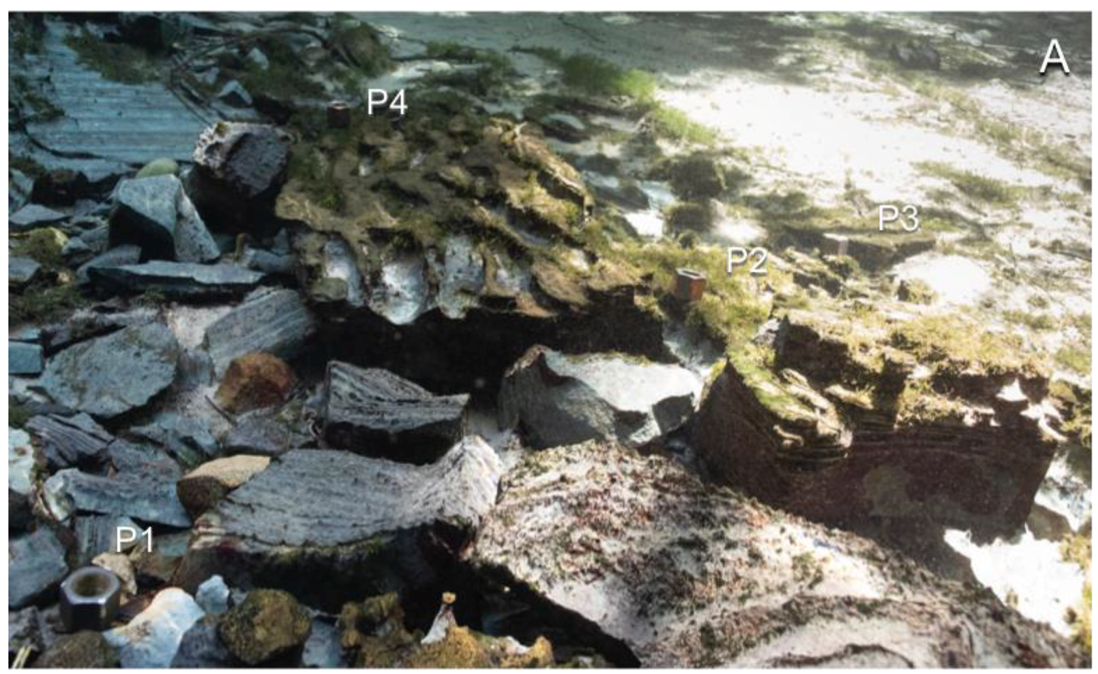
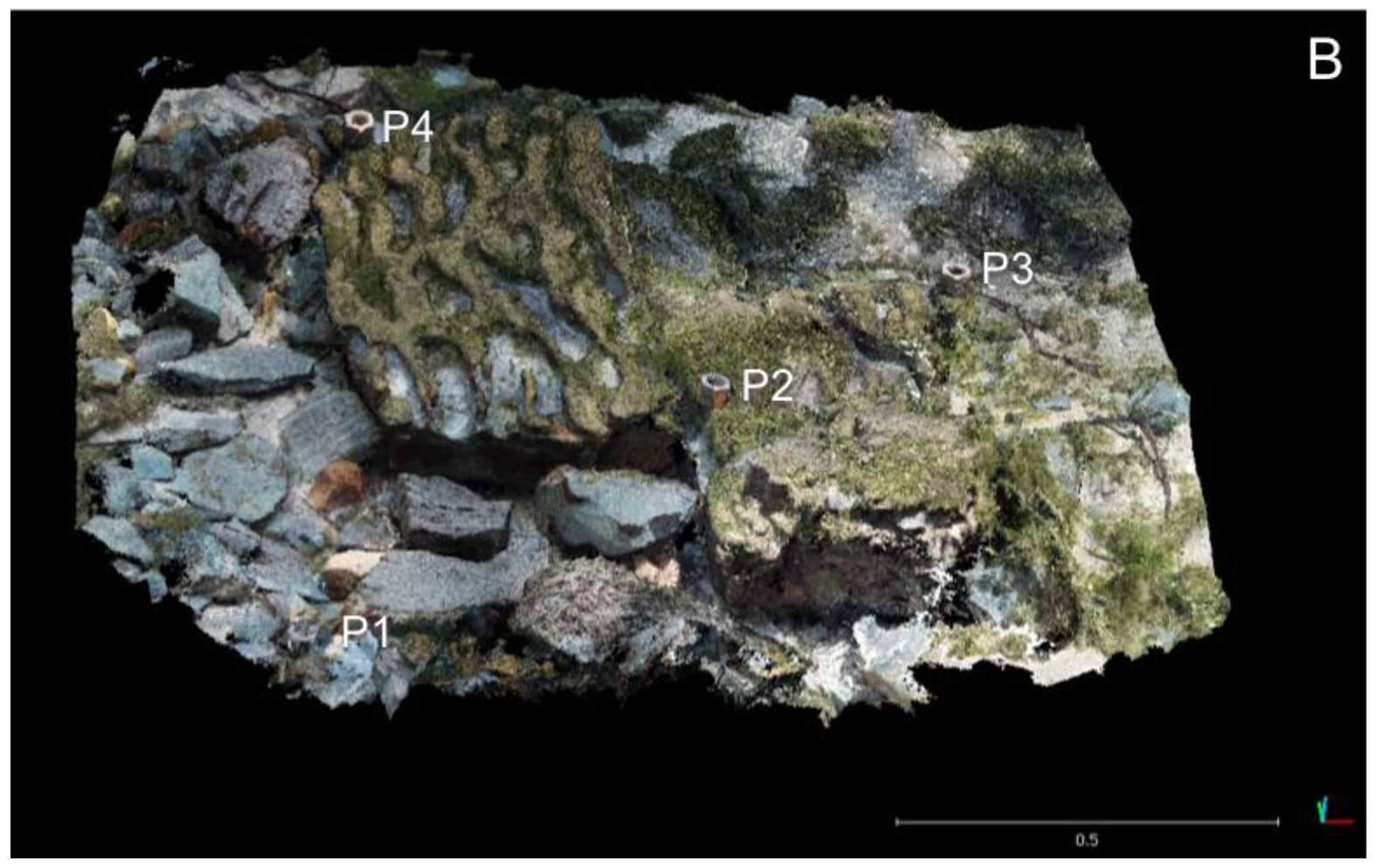
2.6. SfM-MVS Model Assessment

While the accuracy of terrestrial SfM-MVS models has been established using the methods described here (e.g., [13]), a range of accuracies have been reported in the literature for underwater SfM-MVS in marine environments (e.g., [21]) but no quantification of the uncertainties has been published for freshwater ecosystems, which have inherently different structures than coral reefs. Assessment of the submerged DSM from the UAV based SfM-MVS (Inspire 2 UAV and X5S camera—176 photographs) was carried out in controlled conditions (i.e., outdoor swimming pool with a maximum depth of 220 cm) using nine 30 cm diameter targets placed at various depths ranging from the surface to 220 cm deep. Estimated depth from the surface for each target from the dense point cloud was compared to the actual measured depth to the targets. For the underwater SfM-MVS products, the uncertainty of within model measured distances was determined from an underwater substrate reconstruction with stainless steel hexagonal locknuts used as targets (Figure A1). Four hundred photographs were collected in .CR2 with a Canon 1DX Mark II with a 24 mm EF1.2 lens in autofocus mode set to ISO 3200. Linear distance measurements between the hexagonal locknuts were carried out with two divers in snorkel gear and a standard measuring tape. Dimensions of the locknuts were also measured with a digital calliper.

3. Results

We found a strong significant relationship between the UAV based submerged DSM (GSD = 0.65 cm) and the in-situ measurements of the distances between the targets and the surface of the water (R2 = 0.994, Sy.x = 6.205, p < 0.001, F = 1449). While these data were collected under controlled conditions, they represent the range of depths at the Jatobá study site. Table 3 illustrates the results of the underwater SfM-MVS measurements of distance between features in the dense 3D point cloud and measurements taken in-situ. The distance between features measured in the point cloud and in-situ with the tape measure underwater range from 1.4 to 2.5 cm (Table 3, Figure A1). For the measurements of the dimensions of the lock nuts, the difference between the digital calliper and the dense 3D point cloud range from 0.01–0.04 cm.
From the Jatobá site, Figure 7 illustrates the finer spatial resolution obtainable from UAV photography in contrast to best available satellite imagery collected close in time to the UAV data (9 days difference). In the pansharpened GeoEye satellite image (50 cm panchromatic, 2 m multispectral), the location of the largest rapids can be seen but substrate classes cannot be determined (Figure 7a). The glare off the surface of the water also prevents determining other information from the subsurface such the presence of aquatic vegetation. From the UAV photograph (Figure 7b) locations of shallow and deep water can be inferred as well as the outlines of the largest boulders underwater. The flexibility of the UAV operation allows for multiple view angles to minimize glare and optimize the spatial information in each frame. A single aerial frame (Figure 7b) is a flat 2D representation of the surface and lens distortions, variations in depth of field and a lack of coordinates for each pixel of the photograph prevent accurate measurements of area, distance or volume. However, once the full set of photographs for a site is processed through the SfM-MVS workflow (Figure 6), measurements of distance and orientation between objects can be made. Furthermore, the 3D point cloud (Figure 7c) can be rotated on the screen to view the landscape from various perspectives. The 3D representation of the landscape and subsequent products (e.g., DSM, orthomosaic) (Figure 8) are also located in real-world geographical coordinates.
While the underwater substrate topography is not immediately evident from the full area DSM with a large range of elevation values (~25 m) (Figure 8a), when a subsection of the DSM representing a 7 × 7 m area of the aquatic substrate is extracted (Figure 9), it is possible to visualize the topography underwater. The values of the submerged DSM (Figure 9a), following the refractive index correction, represent the distance from the surface (1.52–2.39 m), with brighter pixels indicating structures closer to the surface. The RMS height (standard deviation of the height) was found to be 0.1. Higher values indicate larger variations in height and therefore have been interpreted to mean a potentially rougher substrate [23]. Higher values of slope (Figure 9b) represent the edges of boulders. The rugosity (surface to planar ratio) (Figure 9c) is similar, except the overall slope of the riverbed has been removed and pixels with high values of rugosity are found around and between the largest boulders. Due to the GSD of 1.2 cm, features smaller than that cannot be resolved. The length of the topographic correlation was found to be 54.7 cm (E-W) and 52.3 cm (N-S).
From the underwater SfM-MVS a higher GSD (1 mm) was achieved allowing for a more precise definition of the edges of the underwater structures (e.g., boulders) as well as the location of aquatic vegetation and the presence of green filamentous algae (Figure 10a,b). From aerial photographs it can be difficult to distinguish between underwater vegetation and patches of filamentous algae but the two are clearly separable in the underwater orthomosaic (Figure 10a). The map of rugosity (Figure 10c) illustrates the most complex areas are at the boulder—sand interface. Small holes/depressions in the boulders are also distinguishable. The RMS was found to be 0.15. The length of the topographic correlation was found to be 27 cm (E-W) and 13.5 cm (N-S). When the DSM and rugosity maps are spatially degraded to 3 and 15 cm GSD, increasingly generalized, larger scale patterns of topography and overall complexity are seen. The range of rugosity values also decreases with increasing GSD from a maximum of 262 at 1 mm (Figure 10c) to 1.9 at 15 cm (Figure 10g). The three digital transects (Figure 10h) of SRI resulted in values of 2.44 (A-A’), 2.18 (B—B’) and 2.05 (C—C’) respectively.
The low water of the dry season allowed for the 3D reconstruction of habitat classes in portions of the river that are normally submerged in the wet season (Figure 11). The four sites encompass six of the habitat classes from Table 1 as well as illustrate an example of the white water and deep/turbid classes. The Iriri site (Figure 11a) exhibits the largest heterogeneity of habitat classes including cobbles, solid rock, medium and large boulders. In contrast, the Retroculus site (Figure 11b) and Culuene (Figure 11c) are the most homogenous in terms of the number of habitat classes present.
Based on the confusion matrices (Figure A2), the neural networks separated the habitat classes with a high level of accuracy and minimal potential overfitting. The overall accuracy for all four sites was over 90%. Individual class user and producer accuracies were all > 90% with two exceptions, a shallow water class (UA = 83.3%, PA = 85.6%) at Culuene and the shadow class at Iriri (UA = 63.2%, PA = 32.2%). The results of the neural network classification (Figure 12 and Figure 13) reveal that only the bedrock and shallow water classes are consistently found at the four sites. The shallow water class represents water less than 30 cm deep with the sand and/or gravel assemblage classes mixed together. Classes Podostemaceae and Wet Bedrock, while not included in Table 1 are only found in certain areas of the Xingu basin where there are rapids with a splash zone on the surrounding boulders. In our site they are found at Iriri. The class tree/shrub illustrates areas that are not flooded on a permanent basis. In the wet season when these areas are submerged they provide critical habitat for a range of species (Figure 4). Also evident from the proportions (Figure 12) and spatial distribution (Figure 13) of the classes is the variability between locations. Consistent with the overall complexity of the site (Figure 14), the substrate classifications (Figure 11 and Figure 12) reveal Iriri has the highest diversity of habitat classes (9 classes) and Culuene the least (5 classes). The ‘shadow’ class is not included in this total because it represents areas with topographic features such as the spaces between boulders that are not observable from the SfM-MVS products.
The 3D fractal dimension for the different habitat classes, as calculated from the substrate exposed in the dry season (Figure 14) reveals a natural variability in complexity not only between sites but also within the same class at different sites. For example, the solid rock class from Culuene has a low value of 1.27, whereas the same class from Iriri is more complex with a value of 1.7 due to fissures in the bedrock that are not present in Culuene. Overall, Iriri is the site with the greatest habitat complexity (avg = 1.8), whereas Culuene was found to be the least complex (avg = 1.26).

4. Discussion

We demonstrated that ultrafine resolution spatially explicit information about habitat complexity can be generated from both UAV and underwater photographs with a SfM-MVS workflow. The complexity metrics calculated from the SfM-MVS products are critical analytical tools for gaining insight into the habitat classes necessary for conservation of the local species. As for coral reefs [67], for many freshwater fishes in the Xingu river basin, fine resolution satellite imagery (<2 m) (Figure 7a) is spatially too coarse to extract meaningful habitat complexity information. Furthermore, the orbits of most satellites restrict the revisit times and the time of day images are collected at a given location. Cloud cover is further a challenge when relying on optical satellite imagery in the humid tropics. The low altitude from which UAVs are operated not only improves the spatial resolution of the data but also increases the range of conditions under which photographs can be taken (e.g., uniform cloud cover). Underwater SfM-MVS has additional flexibility because varying the camera settings (e.g., ISO) or the use of artificial illumination such as dive lights can produce high quality photographs even under less than ideal natural illumination conditions [24]. In high energy or dangerous aquatic systems such as rivers with strong current, data collection can be extremely challenging. Both UAVs for areas with shallow water and cameras operated from a boat or by an experienced diver/snorkeler could mitigate these challenges [23].
Based on Table 3, the measurements of distance within the dense 3D point cloud were more similar to the digital calliper than to the tape measure because use of the tape measure underwater is prone to human error. A minimum of two snorkelers were required to use the tape measure and record the values. The strong current added to the difficulties of taking accurate measurements underwater.
From the SfM-MVS workflow, the spatial variability in complexity at individual sites is captured due to the 2D and 3D nature of the products (Figure 9, Figure 10 and Figure 11). In comparison, the SRI is less robust and more subjective. The theoretical SRI from the DSM ranges from 2.05 to 2.44. It does not capture the differences in the cross-section profiles. There is also a high degree of subjectivity depending on where the transect is placed [50]. The 2D map of rugosity is more robust where the entire variability can be summarized by the range of values (1–262).
Similar to [50] we found that as the GSD decreases, the values of rugosity increase in the SfM-MVS products, indicating that at finer GSD more of the structural complexity can be actually measured. This scalability is one of the strengths of SfM-MVS; from products generated at a fine GSD, generalizations of the habitats to coarser scales can be readily achieved. Such scaling is not possible from SRI measured in the field because the chain-and-tape method is calculated at a fixed resolution (i.e., chain-link size) [23].
With terrestrial laser scanner reconstructions of terrain, highly accurate classifications have been achieved for geomorphological classes using multi-scale 3D point cloud classification [68]. For classification of the exposed habitats from the SfM-MVS products we found that colour and topographic and texture metrics combined as predictors in the shallow neural network resulted in high accuracy of the classification (Figure 12 and Figure 13, Figure A2). Location and proportion of the habitat classes can provide important information about the ichthyofauna. For example, in-situ observations indicated that at all sites different species preferentially inhabit the different classes. At Iriri for example, the payara (Hydrolycus armatus) is only found in the main white-water channel. The splash zone on the large boulders next to the main rapids allows for growth of riverweeds (Podostomacae spp.) that adhere to solid surfaces in high flow environments. The endemic parrot pacu (Ossubtus xinguensis) has specialized dentition to feed on them. The wet bedrock and Podostemaceae classes were important to differentiate from the surroundings because not only are the riverweeds a food source for fish but also the wet rocks represent the splash zone from the rapids where Podostemaceae dormant from the previous year may regenerate provided a consistent water source. The trunks and lower branches of the vegetation class may become submerged in the wet season where they provide important habitat for fry and juvenile fishes (e.g., Cichla melaniae) as well as spawning and feeding grounds for species such as Leporinus frederici, Farlowella amazona, Geophagus cf altifrons, Aequidens mikaeli and so forth. The boulder class represents habitat for anostomids (e.g., S. respectus and Synaptolaemus latofasciatus), as well as loricariids (e.g., Pseudacanthicus pirarara) and cichlids (e.g., C. dandara) among others. The gravel assemblage class represents habitat and feeding areas for several species including cichlids (e.g., Crenichla sp. 1, G. argyrostictus, R. xinguensis), anostomids (e.g., Leporinus maculatus) and Serrasalmids (e.g., Myleus setiger). The sand class is further important for stingrays (e.g., P. orbignyi), loricariids (e.g., Limatulichthys spp.) and cichlids (e.g., Teleocichla monogramma) among others.
The 3D fractal dimension is a powerful metric, which allows for quantitative comparisons between habitat classes at multiple sites as well as between sites. This metric is scale invariant and relates complexity, spatial patterns and scale [23]. In order for this metric to be calculated, fine spatial resolution, spatially extensive, digital 3D data are required. From an ultrafine resolution (mm pixel size) underwater photography SfM-MVS derived DSM of an inter-tidal reef, Ref. [23] found that fractal dimension better characterized the roughness of the reef than other conventional measures. Our results reinforce this finding (Figure 14).
Despite the strengths of the SfM-MVS framework presented here, there remain limitations. Both the UAV and underwater photography were collected with a nadir view of the substrate, therefore elements of the substrate such as the underside of overhangs, caves, crevices, or tunnels inside boulders or other structures underneath or between boulders are only partially represented (Figure A1). These elements, especially caves within the piles of boulders or holes inside rocks are important features of the habitat for certain fishes. For example, small loricariids such as Leporacanthicus heterodon are preferentially found in crevices and caves between boulders to avoid predation. Ref. [19] also point out this limitation for SfM-MVS reconstruction of coral colonies. For the UAV based submerged DSM, more sophisticated corrections such the fluid lensing approach [67] for the individual frames used in the SfM-MVS workflow have the potential to further improve the reconstruction of the submerged topography.
Both UAV and underwater photographs can provide a baseline for assessing freshwater habitat complexity. However, it is not an automated process and because of the complex nature of the analysis, a thorough understanding of the camera system is necessary to produce reliable and repeatable digital representations of the habitats. Errors can result in the SfM-MVS products if the most important factors are not considered [19]. A number of factors influence the accuracy of the photogrammetric models and subsequent products (DSM, orthomosaic and metrics of complexity). The various software implementations of the SIFT (or SIFT-like) algorithms rely on distinctive key points (i.e., invariant features) in the photographs. Following steps aimed at improving the initial set of candidate key points and filtering to reject points with low contrast and a strong edge response, the retained key points are robust to varying illumination conditions, view angle, pixel noise and so forth [69].
Similar to terrestrial environments, best practices for photographic data collection for underwater SfM-MVS involve a few major considerations: GSD, depth of field, shutter speed and overlap. The GSD (the distance between two consecutive pixel centres as measured on the ground) is a product of the distance of the camera to the ground/substrate and the focal length of the lens [12]. At a given focal length, increasing the distance between the camera and the substrate will result in a coarser GSD and larger imaging area (Figure 15). Conversely, at a given distance between the camera and substrate, increasing the focal length will result in a finer GSD because each pixel will capture a smaller area (will also result in a smaller imaging area). Overlap in both the along track (direction of travel) and across track (neighbouring lines) directions can be optimized once the GSD and imaging area have been determined. For underwater scenes a high overlap in both directions (~ 80%) is recommended.
Depth of field (DoF), the zone within which the photograph is in focus, depends on the aperture used (e.g., f/8), the distance to the substrate and the focal length of the lens. Narrower apertures result in greater DoF (Figure 16).
In addition to overlap, the DoF is a critical element to maximize photograph quality for underwater SfM-MVS because when as much of the subject (i.e., substrate) in the frames is in focus (i.e., maximizing DoF) it allows for a greater number of keypoints to be generated and retained. A wider angle lens and small aperture will increase DoF. An increase in the ISO (i.e., sensitivity to light) will result in an increase in the shutter speed and aperture, if the aperture cannot be set manually (Figure 17). Under the consistent illumination conditions (clear sky with direct solar illumination—not under overhanging vegetation) the photographs from the stream survey (Figure 10) were collected with a narrow range of f-number (µ = 5.7 ± 0.4, range 5.0–7.1) and shutter speed (µ = 138.3 ± 22.1, range 100–200). For the underwater model of the rock with the hexagonal locknuts (Figure A1), overhanging vegetation with patches of clear views to the sky resulted in a greater range of both f-number (µ = 5.6 ± 1.7, range 3.5–10.0) and shutter speed (µ = 143.8 ± 90.1, range 50–400) used. For the UAV photographs (Figure 17b) the X3 camera consistently used a fixed aperture of f/2.8. An increase in shutter speed due to the glare off the surface of the water at the Retroculus site can be seen with the widest range of shutter speeds. For the X5S camera the aperture varied from f/4.0–f/6.3 at Culuene and f/4.0–f/5.6 at Jatobá.
Given the sensor size of the camera (e.g., full frame vs. micro 4/3), the focal length of the lens and the aperture chosen, the hyperfocal distance can be calculated. This value is the closest distance to the lens which is in focus while maintaining the furthest distance in the photograph acceptably sharp. For example, on a full frame sensor with f/5.6 and a 24 mm focal length, the hyperfocal distance is 3.4 m. Focusing at the hyperfocal distance will result in the foreground (anything closer) being out of focus. With UAV based photographs, generally given altitudes of tens of meters above the tallest features in the landscape (e.g., trees), the entire photograph will be collected within the hyperfocal distance. For example, with a micro 4/3 sensor (such as the X5S), f/5.6 and a 24 mm lens, the hyperfocal distance is 6.9 m. With the 15 mm lens used at Jatobá, the hyperfocal distance ranged from 2.7–3.7 m. At a flight altitude of 30 m AGL (Figure 5a), the entire landscape was within the hyperfocal distance. Underwater, however, if the water is shallow and/or the operator is close to the substrate, care must be taken retain an acceptable focus for as much of each frame as possible. This can be achieved by calculating the DoF given a particular focal length and aperture (Figure 16). The lens can be focused on a section of the substrate that would centre and maximize the DoF over the range of topography.
The shutter speed should be fast enough to freeze motion; this is fundamentally important to ensure the frames are in focus. At least 1/125 sec or faster should be used for underwater photography whenever possible. Photographs should be taken under the brightest illumination conditions available taking into consideration water depth and clarity. And, if possible, flash should be avoided because shadows from the objects or structures created by the flash will change with each perspective from which the frames are taken and reduce the likelihood of matching keypoints. Diffusing the flash from the strobes can help to mitigate the harsh shadows if they must be used. Lastly, variable focal length lenses could result in deterioration of the SfM-MVS model over a fixed focal length lens. However, with the use of a lens with high quality optics, high sharpness, low distortion and low chromatic aberration the difference should be minimal.

5. Conclusions

In conclusion, we have shown the SfM-MVS framework from both UAV and underwater photography can be used to effectively assess freshwater habitat complexity in a robust way. We calculated habitat complexity metrics including rugosity, slope and 3D fractal dimension from the SfM-MVS products. Our results show how these products provide spatially explicit complexity metrics, which are more comprehensive than conventional arbitrary cross sections which may not be representative of the habitat. The shallow neural network classifications of SfM-MVS products of substrate exposed in the dry season resulted in high accuracies across classes allowing us to quantify the proportion of the classes available to the fishes in the wet season. UAV and underwater SfM-MVS is robust for quantifying freshwater habitat classes and complexity and should be chosen whenever possible over conventional methods (e.g., chain-and-tape) because of the repeatability, scalability and multi-dimensional nature of the products. The SfM-MVS products can be used to identify high priority freshwater sectors for conservation, species occurrences and diversity studies to provide a broader indication for overall fish species diversity and provide repeatability for monitoring change over time. We have further discussed best practices for underwater SfM-MVS highlighting differences between underwater and UAV based photography. Despite the Xingu’s unique diversity, the recent implementation of the Belo Monte hydroelectric dam in 2015, will negatively impact some of the very specific habitats [55,70,71,72] as already observed by the authors of this study. As such, our study serves as an example of a simple to implement, yet much needed framework for repeatable and consistent in-situ monitoring of freshwater aquatic habitats.

Author Contributions

Conceptualization, M.K., O.L. and L.S.; methodology, M.K., O.L. and L.S.; formal analysis, M.K.; investigation, M.K., O.L., L.S., T.V., J.P.A.-M; resources, M.K., O.L., L.S. and T.V.; writing—original draft preparation, M.K., O.L., J.P.A.-M., L.S. and T.V; writing—review and editing, M.K., O.L., J.P.A.-M., L.S. and T.V.

Funding

Natural Sciences and Engineering Research Council of Canada, Discovery Grant Program to Kalacska and CNPq Universal Project #486376/2013-3 to Sousa.

Acknowledgments

We would like to thank Damilton Rodrigues da Costa (Dani) for fieldwork assistance and Norma Salcedo and Blake Stoughton from Aquatica for camera housing support.

Conflicts of Interest

The authors declare no conflict of interest. The funders had no role in the design of the study; in the collection, analyses, or interpretation of data; in the writing of the manuscript, or in the decision to publish the results.

Appendix A

Figure A1. (A) Photograph of underwater rock structure used to determine the uncertainty in the dense 3D point cloud. P1–P4 represent the locknuts used as targets. (B) Dense 3D point cloud of the rock structure in ‘a.’ Scale bar is in meters. The interactive point cloud is available at: https://bit.ly/calib_rock.
Remotesensing 10 01912 g0a1aRemotesensing 10 01912 g0a1b
Figure A2. Overall confusion matrix from the neural network classification for (a) Iriri; (b) Culuene; (c) Xadá; (d) Retroculus. PO = Podostemaceae, CO = Cobbles, BR = Bedrock, SH = Shallow water, SD = Shadow, VG = Vegetation, TW = Turbid water, WW = White water, SA = Sand, RA = Gravel Assemblage. Y axis represents the target class, X axis represents the output class.
Remotesensing 10 01912 g0a2aRemotesensing 10 01912 g0a2bRemotesensing 10 01912 g0a2c

References

  1. Hutchinson, G.E. Population studies—Animal ecology and demography—Concluding remarks. Cold Spring Harb. Symp. Quant. Boil. 1957, 22, 415–427. [Google Scholar] [CrossRef]
  2. Vandermeer, J.H. Niche Theory. Annu. Rev. Ecol. Syst. 1972, 3, 107–132. [Google Scholar] [CrossRef]
  3. Yamazaki, D.; Trigg, M.A.; Ikeshima, D. Development of a global similar to 90 m water body map using multi-temporal Landsat images. Remote Sens. Environ. 2015, 171, 337–351. [Google Scholar] [CrossRef] [Green Version]
  4. Gleason, C.J.; Smith, L.C. Toward global mapping of river discharge using satellite images and at-many-stations hydraulic geometry. Proc. Natl. Acad. Sci. USA 2014, 111, 4788–4791. [Google Scholar] [CrossRef] [PubMed] [Green Version]
  5. Pajares, G. Overview and current Status of remote sensing applications based on unmanned aerial vehicles (UAVs). Photogramm. Eng. Remote Sens. 2015, 81, 281–329. [Google Scholar] [CrossRef]
  6. Pimm, S.L.; Alibhai, S.; Bergl, R.; Dehgan, A.; Giri, C.; Jewell, Z.; Joppa, L.; Kays, R.; Loarie, S. Emerging Technologies to Conserve Biodiversity. Trends Ecol. Evol. 2015, 30, 685–696. [Google Scholar] [CrossRef] [PubMed]
  7. Sanchez-Azofeifa, A.; Guzman, J.A.; Campos, C.A.; Castro, S.; Garcia-Millan, V.; Nightingale, J.; Rankine, C. Twenty-first century remote sensing technologies are revolutionizing the study of tropical forests. Biotropica 2017, 49, 604–619. [Google Scholar] [CrossRef]
  8. Anderson, K.; Gaston, K.J. Lightweight unmanned aerial vehicles will revolutionize spatial ecology. Front. Ecol. Environ. 2013, 11, 138–146. [Google Scholar] [CrossRef] [Green Version]
  9. Baxter, P.W.J.; Hamilton, G. Learning to fly: Integrating spatial ecology with unmanned aerial vehicle surveys. Ecosphere 2018, 9. [Google Scholar] [CrossRef]
  10. Linchant, J.; Lisein, J.; Semeki, J.; Lejeune, P.; Vermeulen, C. Are unmanned aircraft systems (UASs) the future of wildlife monitoring? A review of accomplishments and challenges. Mamm. Rev. 2015, 45, 239–252. [Google Scholar] [CrossRef]
  11. Fonstad, M.A.; Dietrich, J.T.; Courville, B.C.; Jensen, J.L.; Carbonneau, P.E. Topographic structure from motion: A new development in photogrammetric measurement. Earth Surf. Process. Landf. 2013, 38, 421–430. [Google Scholar] [CrossRef]
  12. Micheletti, N.; Chandler, J.H.; Lane, S.N. Structure from Motion (SfM) Photogrammetry. In Geomorphological Techniques; British Society for Geomorphology: London, UK, 2015; pp. 2–12. [Google Scholar]
  13. Kalacska, M.; Chmura, G.L.; Lucanus, O.; Bérubé, D.; Arroyo-Mora, J.P. Structure from motion will revolutionize analyses of tidal wetland landscapes. Remote Sens. Environ. 2017, 199, 14–24. [Google Scholar] [CrossRef]
  14. Aguera-Vega, F.; Carvajal-Ramirez, F.; Martinez-Carricondo, P.; Lopez, J.S.H.; Mesas-Carrascosa, F.J.; Garcia-Ferrer, A.; Perez-Porras, F.J. Reconstruction of extreme topography from UAV structure from motion photogrammetry. Measurement 2018, 121, 127–138. [Google Scholar] [CrossRef]
  15. Cunliffe, A.M.; Brazier, R.E.; Anderson, K. Ultra-fine grain landscape-scale quantification of dryland vegetation structure with drone-acquired structure-from-motion photogrammetry. Remote Sens. Environ. 2016, 183, 129–143. [Google Scholar] [CrossRef] [Green Version]
  16. Harwin, S.; Lucieer, A. Assessing the accuracy of georeferenced point clouds produced via multi-view stereopsis from unmanned aerial vehicle (UAV) imagery. Remote Sens. 2012, 4, 1573–1599. [Google Scholar] [CrossRef]
  17. James, M.R.; Robson, S. Straightforward reconstruction of 3D surfaces and topography with a camera: Accuracy and geoscience application. J. Geophys. Res. Earth Surf. 2012, 117. [Google Scholar] [CrossRef] [Green Version]
  18. House, J.E.; Brambilla, V.; Bidaut, L.M.; Christie, A.P.; Pizarro, O.; Madin, J.S.; Dornelas, M. Moving to 3D: Relationships between coral planar area, surface area and volume. PeerJ 2018, 6, e4280. [Google Scholar] [CrossRef] [PubMed]
  19. Bryson, M.; Ferrari, R.; Figueira, W.; Pizarro, O.; Madin, J.; Williams, S.; Byrne, M. Characterization of measurement errors using structure-from-motion and photogrammetry to measure marine habitat structural complexity. Ecol. Evol. 2017, 7, 5669–5681. [Google Scholar] [CrossRef] [PubMed]
  20. Palma, M.; Casado, M.R.; Pantaleo, U.; Cerrano, C. High resolution orthomosaics of African coral reefs: A tool for wide-scale benthic monitoring. Remote Sens. 2017, 9, 705. [Google Scholar] [CrossRef]
  21. Raoult, V.; Reid-Anderson, S.; Ferri, A.; Williamson, J.E. How reliable is structure from motion (SfM) over time and between observers? A case study using coral reef bommies. Remote Sens. 2017, 9, 740. [Google Scholar] [CrossRef]
  22. Young, G.C.; Dey, S.; Rogers, A.D.; Exton, D. Cost and time-effective method for multiscale measures of rugosity, fractal dimension, and vector dispersion from coral reef 3D models. PLoS ONE 2017, 12, e0175341. [Google Scholar] [CrossRef] [PubMed]
  23. Leon, J.X.; Roelfsema, C.M.; Saunders, M.I.; Phinn, S.R. Measuring coral reef terrain roughness using ‘Structure-from-Motion’ close-range photogrammetry. Geomorphology 2015, 242, 21–28. [Google Scholar] [CrossRef]
  24. Robert, K.; Huvenne, V.A.I.; Georgiopoulou, A.; Jones, D.O.B.; Marsh, L.; Carter, G.D.O.; Chaumillon, L. New approaches to high-resolution mapping of marine vertical structures. Sci. Rep. 2017, 7, 9005. [Google Scholar] [CrossRef] [PubMed] [Green Version]
  25. Singh, H.; Roman, C.; Pizarro, O.; Eustice, R.; Can, A. Towards high-resolution imaging from underwater vehicles. Int. J. Robot. Res. 2007, 26, 55–74. [Google Scholar] [CrossRef]
  26. Tamminga, A.; Hugenholtz, C.; Eaton, B.; Lapointe, M. Hyperspatial remote sensing of channel reach morphology and hydraulic fish habitat using an unmanned aerial vehicle (UAV): A first assessment in the context of river research and management. River Res. Appl. 2015, 31, 379–391. [Google Scholar] [CrossRef]
  27. Tamminga, A.D.; Eaton, B.C.; Hugenholtz, C.H. UAS-based remote sensing of fluvial change following an extreme flood event. Earth Surf. Process. Landf. 2015, 40, 1464–1476. [Google Scholar] [CrossRef]
  28. Ferrari, R.; Bryson, M.; Bridge, T.; Hustache, J.; Williams, S.B.; Byrne, M.; Figueira, W. Quantifying the response of structural complexity and community composition to environmental change in marine communities. Glob. Chang. Boil. 2016, 22, 1965–1975. [Google Scholar] [CrossRef] [PubMed]
  29. Fonseca, V.P.; Pennino, M.G.; de Nobrega, M.F.; Oliveira, J.E.L.; Mendes, L.D. Identifying fish diversity hot-spots in data-poor situations. Mar. Environ. Res. 2017, 129, 365–373. [Google Scholar] [CrossRef] [PubMed]
  30. Gonzalez-Rivero, M.; Harborne, A.R.; Herrera-Reveles, A.; Bozec, Y.M.; Rogers, A.; Friedman, A.; Ganase, A.; Hoegh-Guldberg, O. Linking fishes to multiple metrics of coral reef structural complexity using three-dimensional technology. Sci. Rep. 2017, 7, 13965. [Google Scholar] [CrossRef] [PubMed] [Green Version]
  31. Nolan, E.T.; Barnes, D.K.A.; Brown, J.; Downes, K.; Enderlein, P.; Gowland, E.; Hogg, O.T.; Laptikhovsky, V.; Morley, S.A.; Mrowicki, R.J.; et al. Biological and physical characterization of the seabed surrounding Ascension Island from 100–1000 m. J. Mar. Boil. Assoc. UK 2017, 97, 647–659. [Google Scholar] [CrossRef] [Green Version]
  32. Shumway, C.A.; Hofmann, H.A.; Dobberfuhl, A.P. Quantifying habitat complexity in aquatic ecosystems. Freshw. Biol. 2007, 52, 1065–1076. [Google Scholar] [CrossRef]
  33. St Pierre, J.I.; Kovalenko, K.E. Effect of habitat complexity attributes on species richness. Ecosphere 2014, 5, 1–10. [Google Scholar] [CrossRef]
  34. Taniguchi, H.; Tokeshi, M. Effects of habitat complexity on benthic assemblages in a variable environment. Freshw. Biol. 2004, 49, 1164–1178. [Google Scholar] [CrossRef]
  35. Tokeshi, M.; Arakaki, S. Habitat complexity in aquatic systems: Fractals and beyond. Hydrobiologia 2012, 685, 27–47. [Google Scholar] [CrossRef]
  36. Lassau, S.A.; Hochuli, D.F. Effects of habitat complexity on ant assemblages. Ecography 2004, 27, 157–164. [Google Scholar] [CrossRef]
  37. McCormick, M.I. Comparison of field methods for measuring surface-topography and their associations with a tropical reef fish assemblage. Mar. Ecol. Prog. Ser. 1994, 112, 87–96. [Google Scholar] [CrossRef]
  38. Dustan, P.; Doherty, O.; Pardede, S. Digital reef rugosity estimates coral reef habitat complexity. PLoS ONE 2013, 8, e57386. [Google Scholar] [CrossRef] [PubMed]
  39. Gleason, A.C.R. Recovery of coral reef rugosity from stereo image pairs. In Proceedings of the Oceans 2003 Mts/IEEE: Celebrating the Past...Teaming toward the Future, San Diego, CA, USA, 22–26 September 2003; p. 451. [Google Scholar]
  40. Shurin, J.B.; Cottenie, K.; Hillebrand, H. Spatial autocorrelation and dispersal limitation in freshwater organisms. Oecologia 2009, 159, 151–159. [Google Scholar] [CrossRef] [PubMed]
  41. Reichert, J.; Backes, A.R.; Schubert, P.; Wilke, T. The power of 3D fractal dimensions for comparative shape and structural complexity analyses of irregularly shaped organisms. Methods Ecol. Evol. 2017, 8, 1650–1658. [Google Scholar] [CrossRef]
  42. Willis, S.C.; Winemiller, K.O.; Lopez-Fernandez, H. Habitat structural complexity and morphological diversity of fish assemblages in a Neotropical floodplain river. Oecologia 2005, 142, 284–295. [Google Scholar] [CrossRef] [PubMed]
  43. Gorman, O.T.; Karr, J.R. Habitat structure and stream fish communities. Ecology 1978, 59, 507–515. [Google Scholar] [CrossRef]
  44. Buhl-Mortensen, L.; Buhl-Mortensen, P.; Dolan, M.F.J.; Dannheim, J.; Bellec, V.; Holte, B. Habitat complexity and bottom fauna composition at different scales on the continental shelf and slope of northern Norway. Hydrobiologia 2012, 685, 191–219. [Google Scholar] [CrossRef] [Green Version]
  45. Du Preez, C. A new arc-chord ratio (ACR) rugosity index for quantifying three-dimensional landscape structural complexity. Landsc. Ecol. 2015, 30, 181–192. [Google Scholar] [CrossRef]
  46. Ahrenstorff, T.D.; Sass, G.G.; Helmus, M.R. The influence of littoral zone coarse woody habitat on home range size, spatial distribution, and feeding ecology of largemouth bass (Micropterus salmoides). Hydrobiologia 2009, 623, 223–233. [Google Scholar] [CrossRef]
  47. Dias, R.M.; da Silva, J.C.B.; Gomes, L.C.; Agostinho, A.A. Effects of macrophyte complexity and hydrometric level on fish assemblages in a Neotropical floodplain. Environ. Biol. Fish. 2017, 100, 703–716. [Google Scholar] [CrossRef]
  48. Dionne, M.; Folt, C.L. An experimental-analysis of macrophyte growth forms as fish foraging habitat. Can. J. Fish. Aquat. Sci. 1991, 48, 123–131. [Google Scholar] [CrossRef]
  49. Gois, K.S.; Antonio, R.R.; Gomes, L.C.; Pelicice, F.M.; Agostinho, A.A. The role of submerged trees in structuring fish assemblages in reservoirs: Two case studies in South America. Hydrobiologia 2012, 685, 109–119. [Google Scholar] [CrossRef]
  50. Storlazzi, C.D.; Dartnell, P.; Hatcher, G.A.; Gibbs, A.E. End of the chain? Rugosity and fine-scale bathymetry from existing underwater digital imagery using structure-from-motion (SfM) technology. Coral Reefs 2016, 35, 889–894. [Google Scholar] [CrossRef]
  51. Pais, M.P.; Henriques, S.; Costa, M.J.; Cabral, H.N. Improving the “chain and tape” method: A combined topography index for marine fish ecology studies. Ecol. Indic. 2013, 25, 250–255. [Google Scholar] [CrossRef]
  52. Getzin, S.; Wiegand, K.; Schoning, I. Assessing biodiversity in forests using very high-resolution images and unmanned aerial vehicles. Methods Ecol. Evol. 2012, 3, 397–404. [Google Scholar] [CrossRef]
  53. Goulding, M.; Barthem, R.; Ferreira, E.J.G. The Smithsonian Atlas of the Amazon; Smithsonian Books: Washington, DC, USA, 2003; p. 253. [Google Scholar]
  54. Zuluaga-Gomez, M.A.; Fitzgerald, D.B.; Giarrizzo, T.; Winemiller, K.O. Morphologic and trophic diversity of fish assemblages in rapids of the Xingu River, a major Amazon tributary and region of endemism. Environ. Biol. Fish. 2016, 99, 647–658. [Google Scholar] [CrossRef]
  55. Fitzgerald, D.B.; Winemiller, K.O.; Perez, M.H.S.; Sousa, L.M. Using trophic structure to reveal patterns of trait-based community assembly across niche dimensions. Funct. Ecol. 2017, 31, 1135–1144. [Google Scholar] [CrossRef] [Green Version]
  56. Sabaj Perez, M. Where the Xingu bends and will soon break. Am. Sci. 2015, 103, 395–403. [Google Scholar] [CrossRef]
  57. Varella, H.R.; Ito, P.M.M. Crenicichla dandara, new species: The black jacundá from the Rio Xingu (Teleostei: Cichlidae). Proc. Acad. Nat. Sci. Phila. 2018, 166, 1–12. [Google Scholar] [CrossRef]
  58. Dandois, J.P.; Olano, M.; Ellis, E.C. Optimal altitude, overlap, and weather conditions for computer vision UAV estimates of forest structure. Remote Sens. 2015, 7, 13895–13920. [Google Scholar] [CrossRef]
  59. Westaway, R.M.; Lane, S.N.; Hicks, D.M. The development of an automated correction procedure for digital photogrammetry for the study of wide, shallow, gravel-bed rivers. Earth Surf. Process. Landf. 2000, 25, 209–226. [Google Scholar] [CrossRef]
  60. Woodget, A.S.; Carbonneau, P.E.; Visser, F.; Maddock, I.P. Quantifying submerged fluvial topography using hyperspatial resolution UAS imagery and structure from motion photogrammetry. Earth Surf. Process. Landf. 2015, 40, 47–64. [Google Scholar] [CrossRef]
  61. Lowe, D.G. Distinctive image features from scale-invariant keypoints. Int. J. Comput. Vis. 2004, 60, 91–110. [Google Scholar] [CrossRef]
  62. Strecha, C.; von Hansen, W.; Van Gool, L.; Fua, P.; Thoennessen, U. On Benchmarking camera calibration and multi-view stereo for high resolution imagery. In Proceedings of the IEEE Conference on Computer Vision and Pattern Recognition, Anchorage, AK, USA, 23–28 June 2008. [Google Scholar]
  63. Strecha, C.; Bronstein, A.M.; Bronstein, M.M.; Fua, P. LDAHash: Improved matching with smaller descriptors. IEEE Trans. Pattern Anal. Mach. Intell. 2012, 34, 66–78. [Google Scholar] [CrossRef] [PubMed]
  64. Walbridge, S.; Slocum, N.; Pobuda, M.; Wright, D.J. Unified geomorphological analysis workflows with benthic terrain modeler. Geosciences 2018, 8, 94. [Google Scholar] [CrossRef]
  65. Zawada, D.G.; Piniak, G.A.; Hearn, C.J. Topographic complexity and roughness of a tropical benthic seascape. Geophys. Res. Lett. 2010, 37. [Google Scholar] [CrossRef] [Green Version]
  66. Moller, M.F. A scaled conjugate-gradient algorithm for fast supervised learning. Neural Netw. 1993, 6, 525–533. [Google Scholar] [CrossRef]
  67. Chirayath, V.; Earle, S.A. Drones that see through waves—Preliminary results from airborne fluid lensing for centimetre-scale aquatic conservation. Aquat. Conserv. Mar. Freshw. Ecosyst. 2016, 26, 237–250. [Google Scholar] [CrossRef]
  68. Brodu, N.; Lague, D. 3D terrestrial lidar data classification of complex natural scenes using a multi-scale dimensionality criterion: Applications in geomorphology. ISPRS J. Photogramm. Remote Sens. 2012, 68, 121–134. [Google Scholar] [CrossRef] [Green Version]
  69. Smith, M.W.; Carrivick, J.L.; Quincey, D.J. Structure from motion photogrammetry in physical geography. Prog. Phys. Geogr. 2016, 40, 247–275. [Google Scholar] [CrossRef]
  70. Fitzgerald, D.B.; Winemiller, K.O.; Perez, M.H.S.; Sousa, L.M. Seasonal changes in the assembly mechanisms structuring tropical fish communities. Ecology 2017, 98, 21–31. [Google Scholar] [CrossRef] [PubMed]
  71. Winemiller, K.O.; McIntyre, P.B.; Castello, L.; Fluet-Chouinard, E.; Giarrizzo, T.; Nam, S.; Baird, I.G.; Darwall, W.; Lujan, N.K.; Harrison, I.; et al. Balancing hydropower and biodiversity in the Amazon, Congo, and Mekong. Science 2016, 351, 128–129. [Google Scholar] [CrossRef] [PubMed] [Green Version]
  72. Andrade, M.C.; Winemiller, K.O.; Barbosa, P.S.; Fortunati, A.; Chelazzi, D.; Cincinelli, A.; Giarrizzo, T. First account of plastic pollution impacting freshwater fishes in the Amazon: Ingestion of plastic debris by piranhas and other serrasalmids with diverse feeding habits. Environ. Pollut. 2019, 244, 766–773. [Google Scholar] [CrossRef] [PubMed]
Figure 1. Study sites in the Xingu River basin, Brazil. Service layer credits: ESRI, HERE, Garmin, OpenStreetMap contributors and the GIS community.
Remotesensing 10 01912 g001
Figure 2. Example of the seasonal difference in exposed substrate between the dry season (a) and wet season. (b) from the Iriri and Xingu Rivers’ confluence.
Remotesensing 10 01912 g002
Figure 3. Examples of the habitat classes described in Table 1. (a) sand and pebbles with a large proportion of sand; (b) sand and pebbles; (c) cobbles; (d) gravel assemblages; (e) medium boulders; (f) large boulders; (g) solid rock (bedrock); (h) solid rock (textured).
Remotesensing 10 01912 g003
Figure 4. Example of morphological diversity commonly associated with the habitat classes in the Xingu River basin. (a) Hemiodus unimaculatus, (b) Pseudoloricaria laeviscula, (c) Potamotrygon orbigny, (d) Retroculus xinguensis, (e) Geophagus argyrostictus, (f) Teleocichla monogramma, (g) Peckoltia sabaji, (h) Crenicichla sp. ‘xingu 1’, (i) Potamotrygon leopoldi, (j) Sartor respectus, (k) Teleocichla preta, (l) Ossubtus xinguensis, (m) Hypancistrus zebra, (n) Cichla melaniae, (o) Hoplias aimara, (p) Baryancistrus xanthellus, (q) Leporinus tigrinus, (r) Hypomasticus julii, (s) Peckoltia vittata, (t) Scobinancistrus aureatus, (u) Spectracanthicus punctatissimus, (v) Tometes kranponhah, (w) Hydrolycus tatauaia. Photographs are not to scale.
Remotesensing 10 01912 g004
Figure 5. (a) Example of a UAV photograph acquired from 30 m altitude at the Jatobá site used in the SfM-MVS analyses. (b) Example of an underwater photograph collected with the camera housing at the water surface (Jatobá) and the lens facing nadir (Scale not shown).
Remotesensing 10 01912 g005
Figure 6. Flow chart of the analytical steps to generate the products (3D point cloud, textured mesh, DSM and orthomosaic) used as inputs to the calculation of the habitat complexity metrics (slope, rugosity, spatial correlation, 3D fractal dimension). For photographs collected from the UAV, the refractive index correction was applied to the DSM prior to the calculation of the habitat complexity metrics. The sparse and dense point clouds from the Xadá study site are shown to the right of the flowchart along with the position of the photographs used for the analysis. Examples of the DSM and orthomosaic products are shown in the results section.
Remotesensing 10 01912 g006
Figure 7. (a) Pansharpened GeoEye satellite image (50 cm panchromatic, 2 m multispectral) acquired 11 August 2017 of the Jatobá study site. (b) UAV photograph acquired 2 August 2017. (c) Densified 3D point cloud (1.2 cm GSD) generated from UAV SfM-MVS analyses using 375 photographs. The substrate (medium and large boulder classes) is visible in the shallow clear water. The interactive point cloud is available at: https://bit.ly/riojatoba.
Remotesensing 10 01912 g007
Figure 8. DSM and orthomosaic produced from the densified 3D point cloud (Figure 6c).
Remotesensing 10 01912 g008
Figure 9. From the UAV based SfM-MVS products at the Jatobá site: (a) Submerged DSM with refractive index correction applied, (b) Slope, (c) Rugosity expressed as the surface to planar ratio.
Remotesensing 10 01912 g009
Figure 10. From the underwater SfM-MVS at the Jatobá site, (a) Orthomosaic at a GSD of 1 mm. (b) Submerged DSM at a GSD of 1 mm. The lines represent the location of the three transects used to calculate virtual chain-and-tape SRI and (c) Rugosity expressed as the surface to planar ratio at a GSD of 1 mm, (d) Submerged DSM resampled to 3 cm, (e) Rugosity expressed as the surface to planar ratio at 3 cm resolution, (f) Submerged DSM resampled to 15 cm, (g) Rugosity expressed as the surface to planar ratio at 15 cm resolution, (h) Cross sections of the three virtual chain-and-tape transects.
Remotesensing 10 01912 g010
Figure 11. Orthomosaics generated from the UAV photographs of (a) Cachoeira Iriri, (b) Retroculus site, (c) Cachoeira Culuene and (d) Cachoeira do Xadá. Examples of the habitat classes ranging from sand and pebbles to large boulders exposed in the dry season. Areas of deep/turbid water and white water can also be seen. The four interactive 3D point clouds are available at: https://bit.ly/iriri3D, https://bit.ly/retroculus, https://bit.ly/culuene, https://bit.ly/xadarapids.
Remotesensing 10 01912 g011
Figure 12. Proportion of substrate classes at Culuene, Iriri, Retroculus and Xadá as determined from the UAV SfM-MVS products and a neural network classification based on substrate exposed by the low water level of the dry season.
Remotesensing 10 01912 g012
Figure 13. Map of substrate classes from the UAV SfM-MVS products and neural network classification for (a) Iriri; (b) Culuene; (c) Xadá and (d) Retroculus.
Remotesensing 10 01912 g013
Figure 14. The Minkowski–Bouligand fractal dimension (D) as a measure of 3D habitat complexity. Each bar represents one of the first five habitat classes from Table 1. SP = Sand/pebbles, CO = Cobbles, TR = Textured rock, MB = Medium boulders, LB = Large boulders, SR = Solid rock. Dotted lines represent the mean for the site.
Remotesensing 10 01912 g014
Figure 15. Diagram illustrating the effect on GSD of varying either the focal length or the distance between the camera and the substrate.
Remotesensing 10 01912 g015
Figure 16. Given the same distance from the substrate, same focal point and focal length, increasing the aperture (smaller f-number) reduces the DoF. The section of the substrate that falls within the grey box would be in focus. In this illustration, an aperture of f/5.6 results in the entire area of interest of the substrate being in focus, while with f/2.8 the top and base of the boulders would be out of focus.
Remotesensing 10 01912 g016
Figure 17. (a) Violin plots of the shutter speed (blue) and aperture (grey) used to take the photographs for calculating the within model uncertainty (Canon 1DX Mark II) (Figure A1) and for the stream survey (Canon 5D Mark III) (Figure 10). Focal length for both cameras was 24 mm. (b) Violin plots of the shutter speed from the UAV photographs from the five study sites (Figure 1).
Remotesensing 10 01912 g017
Table 1. Summary of the nine habitat classes important for Xingu fish diversity.
Class *Grain SizeDescription and Importance
Sand and pebbles<0.5 cmPreferred by species that feed on invertebrates sifted from the sand but relatively few fishes are consistently found in this class.
Cobbles0.5–2.5 cmSeveral endemics have specialized to feed in this class.
Gravel Assemblage2.5–15 cmAffords protection against predators because caves are too small for larger fishes to enter.
Medium boulders15–50 cmAffords cover to many species and forms caves large enough to be used as breeding sites. In shallow sections of the river this is the most biodiverse class.
Large boulders50–300 cmMany mid-sized fishes prefer shadows created by the large boulders. For the large loricariids, caves must be large enough for adults up to 45 cm TL to protect the nest and brood. Narrow fissures in the large boulders shelter fish assemblages that rarely leave their safety. The compressed body shapes allow species to reside inside the fissures safe from predators (e.g., Ancistrus ranunculus, H. zebra).
Solid rock (bedrock)N/AFew fishes are consistently found in this class. The biocover and algae on the surface provides food to specialized species.
Solid rock (textured)N/AThe shapes and surfaces characteristic of this substrate are ideal hiding places for smaller loricariids.
White waterN/APhotographs (aerial or underwater) cannot be used to determine the substrate in areas of very high flow where the white water of the rapids obscures the river bottom. Some of the most rheophile fishes are consistently found in this class.
Deep turbid waterN/AAdults of the largest fishes of the river (e.g., Brachyplatystoma tigrinum, Phractocephalus hemioliopterus) are not commonly seen in water shallower than 200 cm. Due to the turbidity and/or depth, aerial photographs cannot be used to characterize the substrate in this class.
* The grain sizes of the classes have been modified from the Wentworth scale to reflect the relevance of the classes to the fish species.
Table 2. Summary of UAV photographs collected for the study sites including the ground sampling distance (cm) of the densified 3D point cloud and the number of photographs used for creating the 3D models.
LocationRiverDateUAV CameraArea (ha)GSD (cm)No. Photographs
JatobáJatobá2 August 2017Inspire 2 X5S2.801.20375
Cachoeira CulueneCuluene1 August 2017Inspire 2X5S4.541.75283
Retroculus siteXingu8 August 2016Inspire 1X30.521.43208
Cachoeira XadaXingu11 August 2016Inspire 1X34.622.38420
Cachoeira IririIriri6 August 2016Inspire 1X32.77 1.46425
Table 3. Comparison between measurements from the underwater SfM-MVS model and tape measure distances and digital calliper measurements of the dimensions of the hexagonal locknut targets. P1–P4 refer to the locations of the locknuts in Figure A1. Measurements are in cm.
MeasurementModelIn-SituAbsolute Difference
Tape Measure
P1-P268.466.51.9
P2-P342.441.01.4
P3-P476.975.51.4
P2-P459.357.02.3
P1-P485.082.52.5
Digital Calliper
Width3.613.570.04
Thickness0.670.680.01
Height3.023.010.01

