Automatic Mapping of Thermokarst Landforms from Remote Sensing Images Using Deep Learning: A Case Study in the Northeastern Tibetan Plateau


Abstract
:
1. Introduction
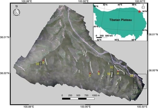
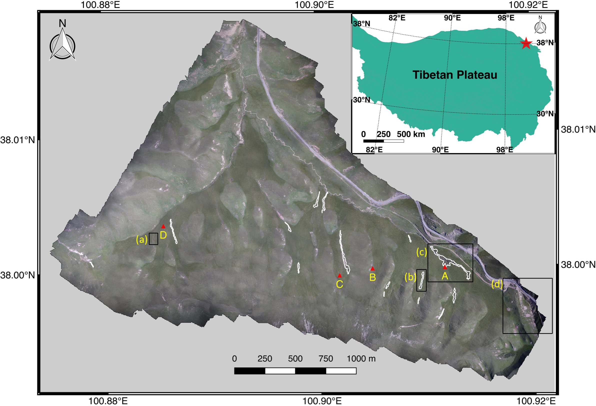
2. Study Area
3. Methods
3.1. Collection of UAV Images and Creation of Digital Orthophoto Map (DOM)
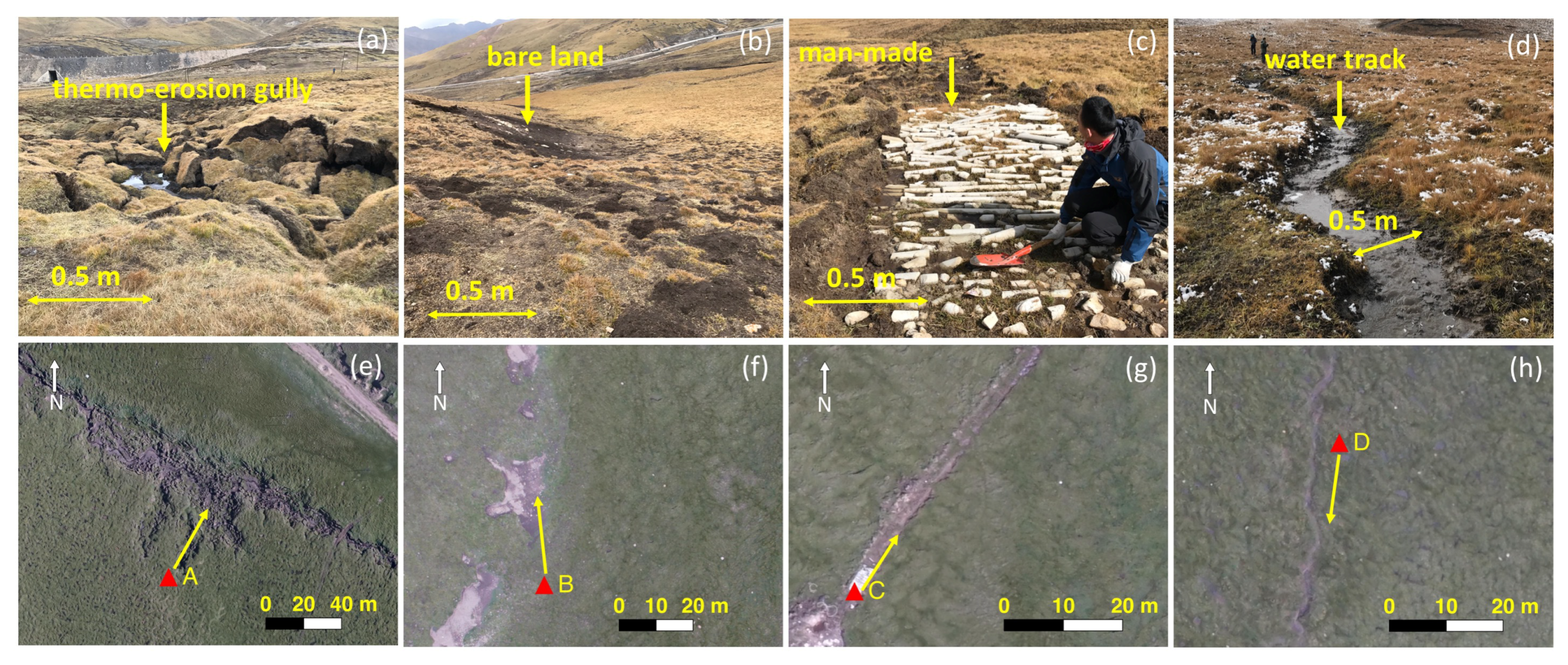
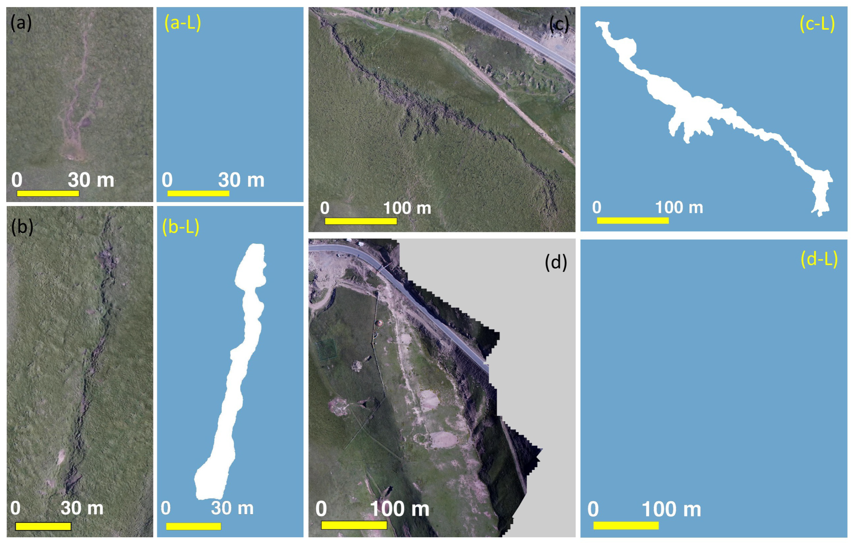
3.2. Collection of Ground Truth Polygons
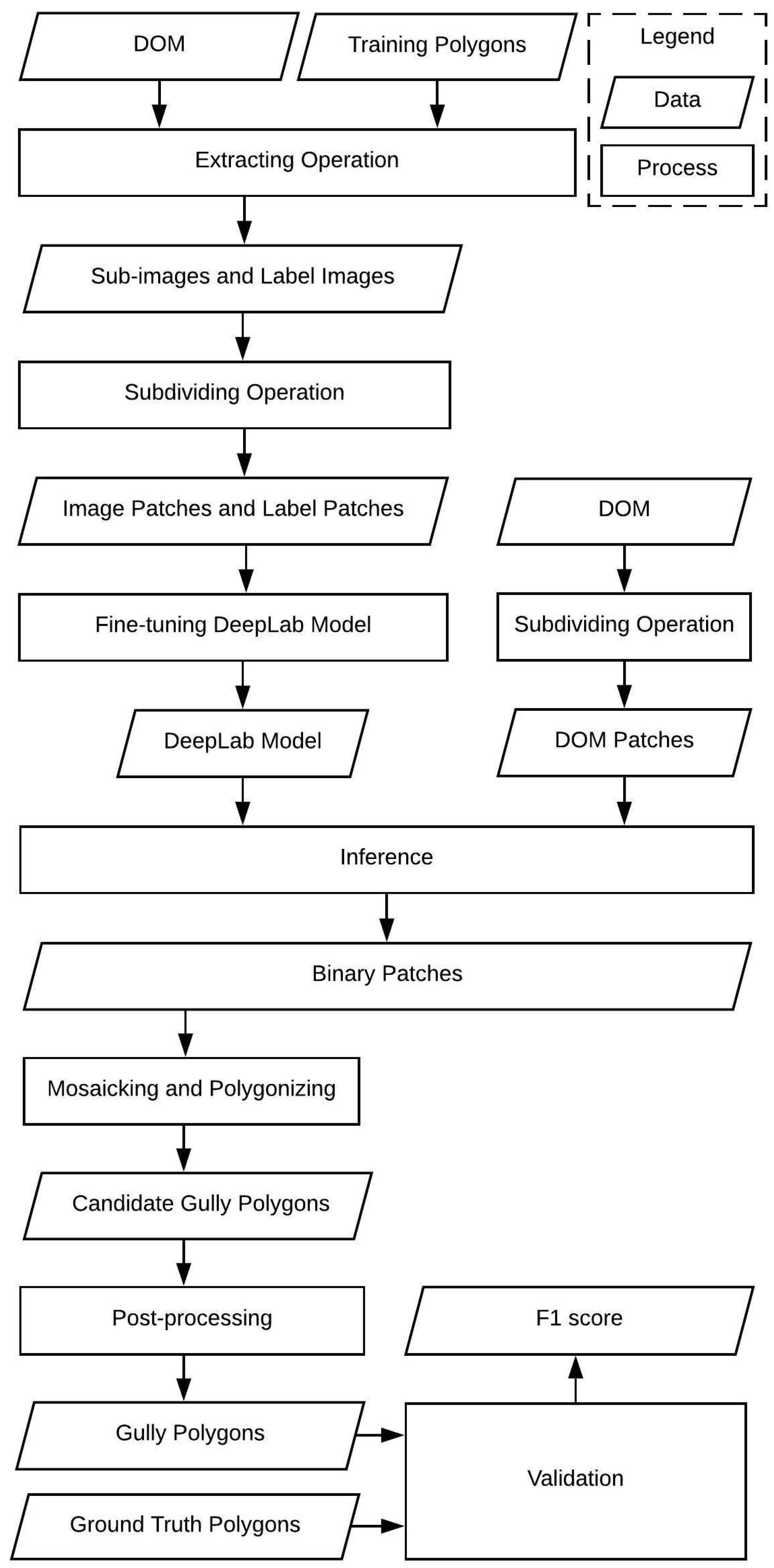
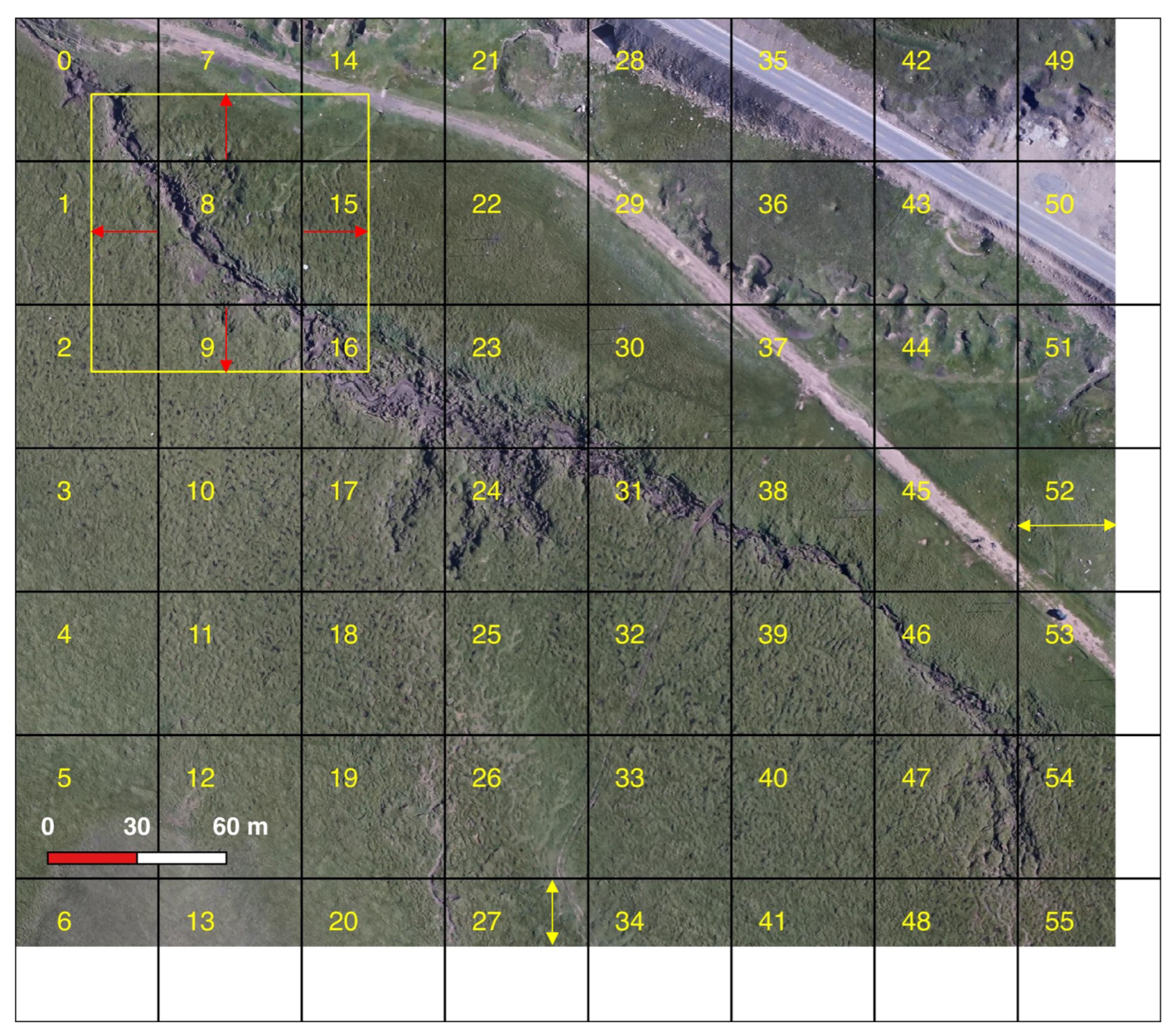
3.3. Preparation of Training Data
3.4. Mapping of Thermo-Erosion Gullies Using DeepLab
3.5. Post-Processing
3.6. Validation
4. Results
5. Discussion
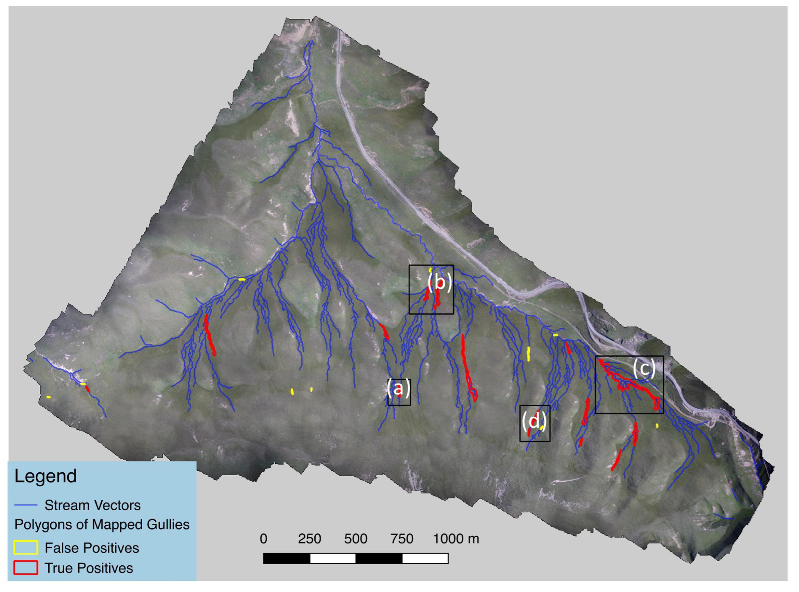
5.1. Spatial Distribution of the Thermo-Erosion Gullies
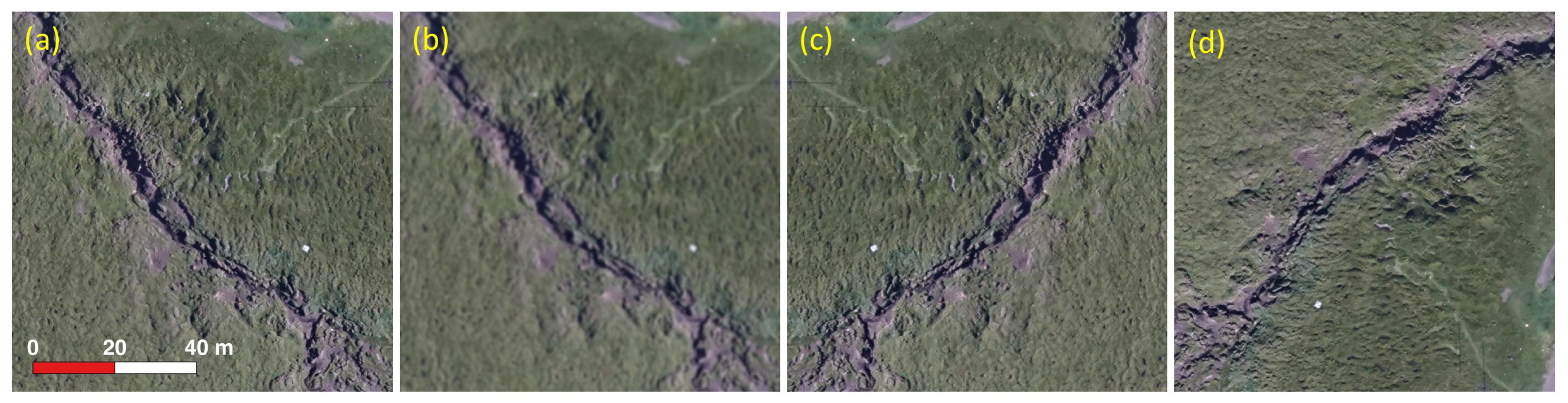
5.2. Delineation Accuracies of the True Positives
5.3. Possible Causes of False Positives
5.4. Mapping of Thermo-Erosion Gullies on the DEM
5.5. Advantages and Limitations of Deep Learning for Mapping Thermokarst Landforms
5.6. Prospects and Future Work for Mapping Thermokarst Landforms in a Large Area
6. Conclusions
Supplementary Materials
Author Contributions
Funding
Acknowledgments
Conflicts of Interest
References
- Zhang, T.; Barry, R.G.; Knowles, K.; Heginbottom, J.A.; Brown, J. Statistics and characteristics of permafrost and ground-ice distribution in the Northern Hemisphere 1. Polar Geogr. 1999, 23, 132–154. [Google Scholar] [CrossRef]
- Marchenko, S.S.; Gorbunov, A.P.; Romanovsky, V.E. Permafrost warming in the Tien Shan mountains, central Asia. Glob. Planet. Chang. 2007, 56, 311–327. [Google Scholar] [CrossRef]
- Osterkamp, T.E. Characteristics of the recent warming of permafrost in Alaska. J. Geophys. Res. Earth Surf. 2007, 112. [Google Scholar] [CrossRef] [Green Version]
- Romanovsky, V.E.; Smith, S.L.; Christiansen, H.H. Permafrost thermal state in the polar Northern Hemisphere during the international polar year 2007–2009: A synthesis. Permafr. Periglac. Process. 2010, 21, 106–116. [Google Scholar] [CrossRef]
- Romanovsky, V.E.; Drozdov, D.S.; Oberman, N.G.; Malkova, G.V.; Kholodov, A.L.; Marchenko, S.S.; Moskalenko, N.G.; Sergeev, D.O.; Ukraintseva, N.G.; Abramov, A.A. Thermal state of permafrost in Russia. Permafr. Periglac. Process. 2010, 21, 136–155. [Google Scholar] [CrossRef] [Green Version]
- Wu, Q.; Zhang, T. Recent permafrost warming on the Qinghai-Tibetan Plateau. J. Geophys. Res. Atmos. 2008, 113. [Google Scholar] [CrossRef] [Green Version]
- Zhao, L.; Wu, Q.; Marchenko, S.S.; Sharkhuu, N. Thermal state of permafrost and active layer in Central Asia during the International Polar Year. Permafr. Periglac. Process. 2010, 21, 198–207. [Google Scholar] [CrossRef]
- Åkerman, H.J.; Johansson, M. Thawing permafrost and thicker active layers in sub-arctic Sweden. Permafr. Periglac. Process. 2008, 19, 279–292. [Google Scholar] [CrossRef]
- Czudek, T.; Demek, J. Thermokarst in Siberia and its influence on the development of lowland relief. Quat. Res. 1970, 1, 103–120. [Google Scholar] [CrossRef]
- Jorgenson, M.T.; Osterkamp, T.E. Response of boreal ecosystems to varying modes of permafrost degradation. Can. J. For. Res. 2005, 35, 2100–2111. [Google Scholar] [CrossRef]
- Jorgenson, M.T. Thermokarst terrains. Treatise Geomorphol. 2013, 8, 313–324. [Google Scholar]
- Shur, Y.L.; Jorgenson, M.T. Patterns of permafrost formation and degradation in relation to climate and ecosystems. Permafr. Periglac. Process. 2007, 18, 7–19. [Google Scholar] [CrossRef]
- Grosse, G.; Harden, J.; Turetsky, M.; McGuire, A.D.; Camill, P.; Tarnocai, C.; Frolking, S.; Schuur, E.A.; Jorgenson, T.; Marchenko, S. Vulnerability of high-latitude soil organic carbon in North America to disturbance. J. Geophys. Res. Biogeosci. 2011, 116. [Google Scholar] [CrossRef] [Green Version]
- Olefeldt, D.; Goswami, S.; Grosse, G.; Hayes, D.; Hugelius, G.; Kuhry, P.; McGuire, A.D.; Romanovsky, V.E.; Sannel, A.B.K.; Schuur, E. Circumpolar distribution and carbon storage of thermokarst landscapes. Nat. Commun. 2016, 7, 13043. [Google Scholar] [CrossRef] [PubMed] [Green Version]
- Schuur, E.; McGuire, A.D.; Schdel, C.; Grosse, G.; Harden, J.W.; Hayes, D.J.; Hugelius, G.; Koven, C.D.; Kuhry, P.; Lawrence, D.M. Climate change and the permafrost carbon feedback. Nature 2015, 520, 171–179. [Google Scholar] [CrossRef] [PubMed]
- Tarnocai, C.; Canadell, J.G.; Schuur, E.; Kuhry, P.; Mazhitova, G.; Zimov, S. Soil organic carbon pools in the northern circumpolar permafrost region. Glob. Biogeochem. Cycles 2009, 23. [Google Scholar] [CrossRef] [Green Version]
- Jorgenson, M.T.; Yoshikawa, K.; Kanevskiy, M.; Shur, Y.; Romanovsky, V.; Marchenko, S.; Grosse, G.; Brown, J.; Jones, B. Permafrost characteristics of Alaska. In Proceedings of the Ninth International Conference on Permafrost, Fairbanks, AK, USA, 20 June–3 July 2008; Volume 3, pp. 121–122. [Google Scholar]
- Fortier, D.; Allard, M.; Shur, Y. Observation of Rapid Drainage System Development by Thermal Erosion of Ice Wedges on Bylot Island, Canadian Arctic Archipelago. Permafr. Periglac. Process. 2007, 18, 229–243. [Google Scholar] [CrossRef]
- Luo, J.; Niu, F.; Lin, Z.; Liu, M.; Yin, G. Thermokarst lake changes between 1969 and 2010 in the Beilu River Basin, Qinghai–Tibet Plateau, China. Sci. Bull. 2015, 60, 556–564. [Google Scholar] [CrossRef]
- Niu, F.; Lin, Z.; Lu, J.; Luo, J.; Wang, H. Assessment of terrain susceptibility to thermokarst lake development along the Qinghai–Tibet engineering corridor, China. Environ. Earth Sci. 2015, 73, 5631–5642. [Google Scholar] [CrossRef]
- Ramage, J.L.; Irrgang, A.M.; Herzschuh, U.; Morgenstern, A.; Couture, N.; Lantuit, H. Terrain controls on the occurrence of coastal retrogressive thaw slumps along the Yukon Coast, Canada. J. Geophys. Res. Earth Surf. 2017, 122, 1619–1634. [Google Scholar] [CrossRef]
- Nitze, I.; Grosse, G. Detection of landscape dynamics in the Arctic Lena Delta with temporally dense Landsat time-series stacks. Remote Sens. Environ. 2016, 181, 27–41. [Google Scholar] [CrossRef]
- Nitze, I.; Grosse, G.; Jones, B.M.; Arp, C.D.; Ulrich, M.; Fedorov, A.; Veremeeva, A. Landsat-based trend analysis of lake dynamics across northern permafrost regions. Remote Sens. 2017, 9, 640. [Google Scholar] [CrossRef]
- Lacelle, D.; Brooker, A.; Fraser, R.H.; Kokelj, S.V. Distribution and growth of thaw slumps in the Richardson Mountains–Peel Plateau region, northwestern Canada. Geomorphology 2015, 235, 40–51. [Google Scholar] [CrossRef]
- Godin, E.; Fortier, D. Geomorphology of thermo-erosion gullies–case study from Bylot Island, Nunavut, Canada. In Proceedings of the 6th Canadian Permafrost Conference and 63rd Canadian Geotechnical Conference, Calgary, AB, Canada, 12–16 September 2010; pp. 1540–1547. [Google Scholar]
- Godin, E.; Fortier, D. Fine Scale Spatio-Temporal Monitoring of Multiple Thermo-Erosion Gullies Development on Bylot Island, Eastern Canadian Archipelago. In Proceedings of the Tenth International Conference on Permafrost (TICOP), Salekhard, Russia, 25–29 June 2012; Volume 1, pp. 1–7. [Google Scholar]
- Belshe, E.F.; Schuur, E.; Grosse, G. Quantification of upland thermokarst features with high resolution remote sensing. Environ. Res. Lett. 2013, 8, 035016. [Google Scholar] [CrossRef] [Green Version]
- Rudy, A.C.; Lamoureux, S.F.; Treitz, P.; Collingwood, A. Identifying permafrost slope disturbance using multi-temporal optical satellite images and change detection techniques. Cold Reg. Sci. Technol. 2013, 88, 37–49. [Google Scholar] [CrossRef]
- LeCun, Y.; Bottou, L.; Bengio, Y.; Haffner, P. Gradient-based learning applied to document recognition. Proc. IEEE 1998, 86, 2278–2324. [Google Scholar] [CrossRef] [Green Version]
- Krizhevsky, A.; Sutskever, I.; Hinton, G.E. Imagenet classification with deep convolutional neural networks. In Proceedings of the Advances in Neural Information Processing Systems, Lake Tahoe, NY, USA, 3–8 December 2012; pp. 1097–1105. [Google Scholar]
- LeCun, Y.; Bengio, Y.; Hinton, G. Deep learning. Nature 2015, 521, 436–444. [Google Scholar] [CrossRef]
- Silver, D.; Schrittwieser, J.; Simonyan, K.; Antonoglou, I.; Huang, A.; Guez, A.; Hubert, T.; Baker, L.; Lai, M.; Bolton, A. Mastering the game of Go without human knowledge. Nature 2017, 550, 354–359. [Google Scholar] [CrossRef]
- Guo, W.; Yang, W.; Zhang, H.; Hua, G. Geospatial Object Detection in High Resolution Satellite Images Based on Multi-Scale Convolutional Neural Network. Remote Sens. 2018, 10, 131. [Google Scholar] [CrossRef]
- Huang, B.; Zhao, B.; Song, Y. Urban land-use mapping using a deep convolutional neural network with high spatial resolution multispectral remote sensing imagery. Remote Sens. Environ. 2018, 214, 73–86. [Google Scholar] [CrossRef]
- Jean, N.; Burke, M.; Xie, M.; Davis, W.M.; Lobell, D.B.; Ermon, S. Combining satellite imagery and machine learning to predict poverty. Science 2016, 353, 790–794. [Google Scholar] [CrossRef] [PubMed]
- Zhu, X.X.; Tuia, D.; Mou, L.; Xia, G.S.; Zhang, L.; Xu, F.; Fraundorfer, F. Deep Learning in Remote Sensing: A Comprehensive Review and List of Resources. IEEE Geosci. Remote Sens. Mag. 2017, 5, 8–36. [Google Scholar] [CrossRef] [Green Version]
- Mu, C.; Zhang, T.; Cao, B.; Wan, X.; Peng, X.; Cheng, G. Study of the organic carbon storage in the active layer of the permafrost over the Eboling Mountain in the upper reaches of the Heihe River in the Eastern Qilian Mountains. J. Glaciol. Geocryol. 2013, 35, 1–9. [Google Scholar]
- Mu, C.; Zhang, T.; Wu, Q.; Cao, B.; Zhang, X.; Peng, X.; Wan, X.; Zheng, L.; Wang, Q.; Cheng, G. Carbon and nitrogen properties of permafrost over the Eboling Mountain in the upper reach of Heihe River basin, Northwestern China. Arct. Antarct. Alpine Res. 2015, 47, 203–211. [Google Scholar] [CrossRef]
- Mu, C.; Abbott, B.W.; Wu, X.D.; Zhao, Q.; Wang, H.J.; Su, H.; Wang, S.F.; Gao, T.G.; Guo, H.; Peng, X.Q. Thaw Depth Determines Dissolved Organic Carbon Concentration and Biodegradability on the Northern Qinghai-Tibetan Plateau. Geophys. Res. Lett. 2017, 44, 9389–9399. [Google Scholar] [CrossRef]
- Wang, Q.F.; Zhang, T.J.; Wu, J.C.; Peng, X.Q.; Zhong, X.Y.; Mu, C.C.; Wang, K.; Wu, Q.B.; Cheng, G.D. Investigation on permafrost distribution over the upper reaches of the Heihe River in the Qilian Mountains. J. Glaciol. Geocryol. 2013, 35, 19–25. [Google Scholar]
- Cao, B.; Gruber, S.; Zhang, T.; Li, L.; Peng, X.; Wang, K.; Zheng, L.; Shao, W.; Guo, H. Spatial variability of active layer thickness detected by ground-penetrating radar in the Qilian Mountains, Western China. J. Geophys. Res. Earth Surf. 2017, 122, 574–591. [Google Scholar] [CrossRef]
- Cao, B.; Zhang, T.; Peng, X.; Mu, C.; Wang, Q.; Zheng, L.; Wang, K.; Zhong, X. Thermal Characteristics and Recent Changes of Permafrost in the Upper Reaches of the Heihe River Basin, Western China. J. Geophys. Res. Atmos. 2018, 123, 7935–7949. [Google Scholar] [CrossRef]
- Mu, C.; Zhang, T.; Zhang, X.; Li, L.; Guo, H.; Zhao, Q.; Cao, L.; Wu, Q.; Cheng, G. Carbon loss and chemical changes from permafrost collapse in the northern Tibetan Plateau. J. Geophys. Res. Biogeosci. 2016, 121, 1781–1791. [Google Scholar] [CrossRef]
- Everingham, M.; Eslami, S.A.; Gool, L.V.; Williams, C.K.; Winn, J.; Zisserman, A. The pascal visual object classes challenge: A retrospective. Int. J. Comput. Vis. 2015, 111, 98–136. [Google Scholar] [CrossRef]
- Chen, L.C.; Papandreou, G.; Kokkinos, I.; Murphy, K.; Yuille, A.L. Deeplab: Semantic image segmentation with deep convolutional nets, atrous convolution, and fully connected crfs. arXiv, 2016; arXiv:1606.00915. [Google Scholar] [CrossRef] [PubMed]
- Goodfellow, I.; Bengio, Y.; Courville, A.; Bengio, Y. Deep Learning; MIT Press: Cambridge, UK, 2016; Volume 1. [Google Scholar]
- Castelvecchi, D. Can we open the black box of AI? Nat. News 2016, 538, 20. [Google Scholar] [CrossRef] [PubMed]
- Zeiler, M.D.; Fergus, R. Visualizing and understanding convolutional networks. In Proceedings of the European conference on computer vision, Zurich, Switzerland, 6–12 September 2014; Springer: Cham, Switzerland, 2014; pp. 818–833. [Google Scholar]
- Council, N.R. Opportunities to Use Remote Sensing in Understanding Permafrost and Related Ecological Characteristics: Report of a Workshop; National Academies Press: Washington, DC, USA, 2014. [Google Scholar]


| Group | # | TP | FP | FN | Precision | Recall | F1 Score |
|---|---|---|---|---|---|---|---|
| 1 | 1 | 16 | 17 | 0 | 0.48 | 1.00 | 0.65 |
| 2 | 2 | 12 | 15 | 4 | 0.44 | 0.75 | 0.56 |
| 3 | 13 | 13 | 3 | 0.50 | 0.81 | 0.62 | |
| 4 | 14 | 12 | 2 | 0.54 | 0.88 | 0.67 | |
| 5 | 15 | 18 | 1 | 0.45 | 0.94 | 0.61 | |
| 6 | 13 | 22 | 3 | 0.37 | 0.81 | 0.51 | |
| 7 | 15 | 17 | 1 | 0.47 | 0.94 | 0.63 | |
| 8 | 15 | 15 | 1 | 0.50 | 0.94 | 0.65 | |
| 9 | 12 | 22 | 4 | 0.35 | 0.75 | 0.48 | |
| 10 | 15 | 20 | 1 | 0.43 | 0.94 | 0.59 | |
| 11 | 14 | 15 | 2 | 0.48 | 0.88 | 0.62 | |
| 3 | 12 | 13 | 24 | 3 | 0.35 | 0.81 | 0.49 |
| 13 | 13 | 21 | 3 | 0.38 | 0.81 | 0.52 | |
| 14 | 13 | 22 | 3 | 0.37 | 0.81 | 0.51 | |
| 15 | 14 | 22 | 2 | 0.39 | 0.88 | 0.54 | |
| 16 | 15 | 7 | 1 | 0.68 | 0.94 | 0.79 | |
| 17 | 13 | 16 | 3 | 0.45 | 0.81 | 0.58 | |
| 18 | 15 | 21 | 1 | 0.42 | 0.94 | 0.58 | |
| 19 | 12 | 8 | 4 | 0.60 | 0.75 | 0.67 | |
| 20 | 13 | 13 | 3 | 0.50 | 0.81 | 0.62 | |
| 21 | 15 | 13 | 1 | 0.54 | 0.94 | 0.68 |
© 2018 by the authors. Licensee MDPI, Basel, Switzerland. This article is an open access article distributed under the terms and conditions of the Creative Commons Attribution (CC BY) license (http://creativecommons.org/licenses/by/4.0/).
Share and Cite
Huang, L.; Liu, L.; Jiang, L.; Zhang, T. Automatic Mapping of Thermokarst Landforms from Remote Sensing Images Using Deep Learning: A Case Study in the Northeastern Tibetan Plateau. Remote Sens. 2018, 10, 2067. https://0-doi-org.brum.beds.ac.uk/10.3390/rs10122067
Huang L, Liu L, Jiang L, Zhang T. Automatic Mapping of Thermokarst Landforms from Remote Sensing Images Using Deep Learning: A Case Study in the Northeastern Tibetan Plateau. Remote Sensing. 2018; 10(12):2067. https://0-doi-org.brum.beds.ac.uk/10.3390/rs10122067
Chicago/Turabian StyleHuang, Lingcao, Lin Liu, Liming Jiang, and Tingjun Zhang. 2018. "Automatic Mapping of Thermokarst Landforms from Remote Sensing Images Using Deep Learning: A Case Study in the Northeastern Tibetan Plateau" Remote Sensing 10, no. 12: 2067. https://0-doi-org.brum.beds.ac.uk/10.3390/rs10122067