Retrieval of Chlorophyll a from Sentinel-2 MSI Data for the European Union Water Framework Directive Reporting Purposes


Tartu Observatory, University of Tartu, Observatooriumi 1, Tõravere, Nõo parish, 61602 Tartu County, Estonia
*
Author to whom correspondence should be addressed.
Remote Sens. 2019, 11(1), 64; https://0-doi-org.brum.beds.ac.uk/10.3390/rs11010064
Submission received: 12 November 2018
/
Revised: 14 December 2018
/
Accepted: 19 December 2018
/
Published: 31 December 2018
(This article belongs to the Special Issue Understanding the Complexity of Coastal and Inland Waters using Remote Sensing)
Abstract
:The European Parliament and The Council of the European Union have established the Water Framework Directive (2000/60/EC) for all European Union member states to achieve, at least, “good” ecological status of all water bodies larger than 50 hectares in Europe. The MultiSpectral Instrument onboard European Space Agency satellite Sentinel-2 has suitable 10, 20, 60 m spatial resolution to monitor most of the Estonian lakes as required by the Water Framework Directive. The study aims to analyze the suitability of Sentinel-2 MultiSpectral Instrument data to monitor water quality in inland waters. This consists of testing various atmospheric correction processors to remove the influence of atmosphere and comparing and developing chlorophyll a algorithms to estimate the ecological status of water in Estonian lakes. This study shows that the Sentinel-2 MultiSpectral Instrument is suitable for estimating chlorophyll a in water bodies and tracking the spatial and temporal dynamics in the lakes. However, atmospheric corrections are sensitive to surrounding land and often fail in narrow and small lakes. Due to that, deriving satellite-based chlorophyll a is not possible in every case, but initial results show the Sentinel-2 MultiSpectral Instrument could still provide complementary information to in situ data to support Water Framework Directive monitoring requirements.
1. Introduction
Water Framework Directive (2000/60/EC) (WFD) obligates all European Union (EU) member states to implement water management and estimate ecological status in water bodies, through monitoring and classification [1]. The WFD aims to achieve, at least, “good” ecological status of inland waters by 2027, by using a program of measures or maintain the “good” status if it already exists [2]. The classification of ecological status is divided into five categories: “very good” to “very bad”, where category “good” indicates very light bias due to human activity from reference conditions [3,4].
Consistent monitoring in water bodies is essential for fulfilling EU WFD, but traditional in situ monitoring (e.g., water sample collection and later analysis in the laboratory) is a rather time and money consuming method for estimating the quality of water on a regular basis. Since the late 1970s, due to successful ocean color satellite missions, the use of remote sensing technologies has increased [5,6,7], providing possibilities for observing water bodies regularly, locally and globally [8]. The advantages of remote sensing over traditional monitoring methods are temporal and spatial coverage and the possibility to estimate water quality in non-accessible water bodies [6,9,10]. Furthermore, the possibility to compose time series from historical data allows evaluating the changes in water quality over time [11]. However, passive satellite remote sensing is dependent upon weather, air mass changes, and sunlight conditions, which directly affect the quality and quantity of useful data.
Chlorophyll a (chl a) is the main pigment in phytoplankton, which is known as one of the key parameters of the WFD which indicates the trophic status of water. Through photosynthesis, the phytoplankton converts CO2 and H2O into O2 and is responsible for primary production in the water column [6,12]. In addition, chl a is the main indicator of phytoplankton biomass [13,14,15] and can be used to determine the water clarity [9]. Phytoplankton blooms are natural processes in the water environment, which show the normal functioning of a water ecosystem [16]. However, toxic cyanobacteria blooms or the excessive blooms caused by human impact cause environmental problems affecting inland waters directly through the reduction of water quality and indirectly restricting the use of drinking water, fishing, and swimming [17].
Satellite remote sensing has been used as a valuable tool for supporting the implementation of the WFD, by deriving phytoplankton and cyanobacterial pigments such as chl a and phycocyanin (PC), total suspended matter (TSM), colored dissolved organic matter (CDOM), and the spectral attenuation coefficient (Kd) [18]. Gohin et al. [19] have compared in situ data for 74 coastal water bodies with Sea-viewing Wide Field Instrument Sensor (SeaWiFS) images from the period of 1998 to 2004 to estimate annual cycles of the fortnight chl a concentration for implementing WFD requirements by estimating the ecological status of water by chl a. However, results showed notable differences between in situ data and satellite data, which could have been caused by influence from the coastline, resolution or approximation of used methods. For large lakes, Medium Resolution Imaging Spectrometer (MERIS) images have been successfully used for estimating the water quality parameters required by the WFD over optically very different lakes, e.g., in perialpine lakes [20] and in oligotrophic to hyper eutrophic Nordic lakes [21]. Results showed the possibility to estimate the trophic status of different water bodies and trends of chl a seasonal dynamics. Philipson et al. [22] have pointed out, based on the study of Swedish lakes, the limitation of insufficient spatial resolution (300 m) for monitoring smaller lakes required by the WFD. Ocean Color and Land Imager (OLCI) onboard Sentinel-3 (S3), as a continuation for MERIS, has benefits for monitoring large surface water bodies because of similarity to the MERIS sensor and the ability to use previously developed algorithms [23]. The MultiSpectral Instrument (MSI) onboard Sentinel-2 (S2) with high resolution (up to 10 m) has shown suitability for detecting cyanobacterial blooms and retrieval of chl a concentrations in subalpine lakes [24]. However, further development for atmospheric correction (AC) algorithms and the need for the larger validation data over optically complex waters is necessary [25]. Therefore, the EU’s Copernicus Program provides full and free access for quality-controlled data, which is an important source of information for environmental monitoring, and consistent technological improvement [26].
Different aspects have to be considered while deriving water quality parameters from remotely sensed data. According to Morel and Prieur [27], Case 1 waters are mostly dominated by phytoplankton, whereas Case 2 waters with different concentrations of optically active substances (OAS) (chl a, CDOM, TSM) are more complex when deriving water quality parameters. This is due to high and independent absorption and scattering by all OASs [15,28,29]. In addition, as 90% of the signal that reaches the sensor is affected by the absorption and scattering by different particles in the atmosphere (water vapour, ozone, oxygen, carbon dioxide) and aerosols, atmospheric correction (AC) is an essential procedure. Optical sensors measure reflected light from the atmosphere and the surface of the water body at visible (VIS) and near-infrared (NIR) wavelengths. AC processors remove the scattered signal of atmosphere and retrieve the signal from the water’s surface, which is called water-leaving reflectance (ρw) [6,30]. For Case 1 waters, AC algorithms assume that the water-leaving radiance (L) is zero in the NIR part of the spectrum. This assumption is not valid in turbid Case 2 waters because of the scattering by particles that increase the ρw in the NIR part. It causes over-correction in the visible part of the ρw spectrum [31,32]. In small narrow lakes or in the vicinity of the coast, the adjacency effect also influences the reflected light field because pixels are affected by the signal originating from the surrounding land [33]. Pixels from the coastline are brighter than water pixels, and the multiple scattering precludes accurate derivation of water quality parameters [34].
As chl a has absorption peaks in VIS part of the spectrum, it is possible to estimate chl a in remote sensing applications through model-based or empirical approaches. A model-based approach is using bio-optical models to simulate ρw or the top-of-atmosphere (TOA) radiance spectrum with specified water constituents. A more widely empirical approach is used, which is based on band ratios and, therefore, might have a smaller sensitivity, but is easier to develop and apply [6,32].
For Case 1 oceanic waters, the Blue–Green Two-Band Ratio Model (Equation (1)) algorithms work most successfully, because of the phytoplankton domination [13]. The model uses blue–green wavelengths (440–550 nanometers (nm)) because the first absorption peak of chl a is around 440 nm ( and minimal absorption is around 550 nm [27]:
For Case 2 waters, algorithms at blue–green wavelengths fail because of absorption and scattering due to CDOM and TSM [35]. Due to the second chl a absorption peak near 675 nm, the Two-Band NIR–Red Ratio Model (Equation (2)) [36] is widely used, where is located in the range of maximum chl a absorption between 660 and 690 nm and characterizes the range of wavelengths between 700 and 720 nm (), or wavelengths beyond 710 nm ( [10,37].
For more turbid and productive waters the Three-Band NIR–Red Ratio Model (Equation (3)) algorithm has been developed [38], because of a wide range of OAS in the water. The three-Band NIR–Red Ratio Model algorithm uses the same wavelengths as the Two-Band NIR–Red Ratio Model algorithm, where is maximally sensitive to the absorption peak of chl a, is minimally sensitive to the absorption of chl a and is minimally affected by the absorption of chl a [39].
For highly turbid waters Le [40] has done further development for the Three-Band NIR–Red Model and has added into the equation. In the Four-Band NIR–Red Model (Equation (4)) algorithm the fourth band should minimize the impact of absorption and backscattering of TSM in and is located at NIR wavelengths:
Additionally, various so-called line height algorithms have been developed. For detecting surface blooms and near-surface vegetation in coastal and ocean waters, the Maximum Chlorophyll Index (MCI) (Equation (5)) has been used for MERIS sensor, which is based on the height of the peak at 709 nm and is used with chl a over 10 mg/m3 [41]:
In the MCI algorithm, L represents TOA radiance at the specific wavelengths, and the index 0.389 represents the ratio of wavelengths (709 − 681)/(753 − 681). According to Gower [41], the MCI algorithm can be used effectively with ρw values as well, instead of radiances.
The Fluorescence Line Height (FLH) (Equation (6)) algorithm is the most suitable for waters where chl a concentration is 1–20 mg/m3 and it uses the chl a fluorescence peak maximum near 685 nm, that is located between the linear baseline of two adjacent bands [42]:
In the FLH algorithm, L681 is the water-leaving radiance at the fluorescence maximum peak wavelength of MERIS band and the index 0.364 represents the ratio of wavelengths (681 − 665)/(709 − 665).
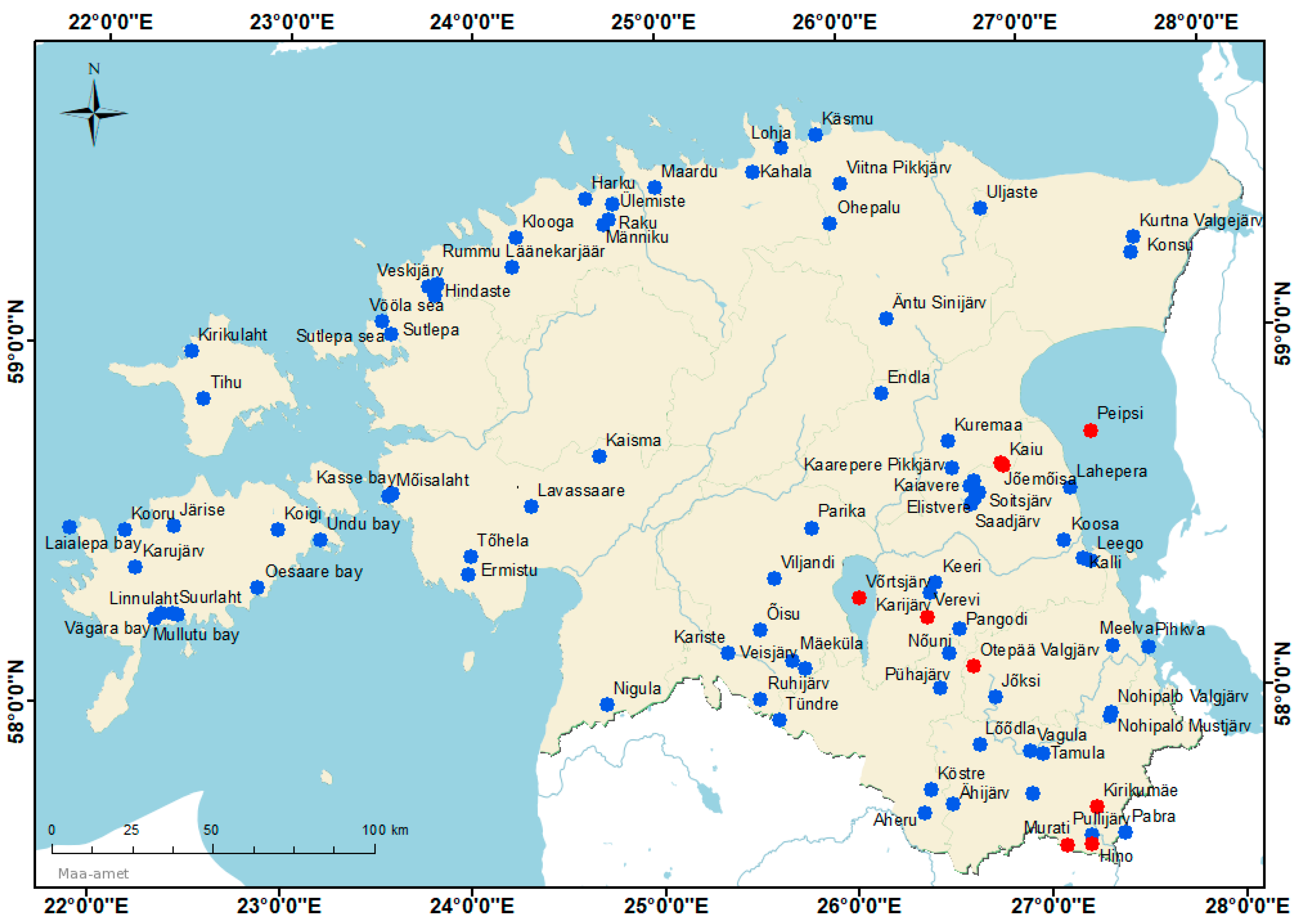
Estonian inland waters are classified as Case 2 waters because of the high amount of different OAS. According to the EU WFD regulations, 89 lakes should be monitored regularly in Estonia (Figure 1), which are divided into eight different groups by the type of water body (Table 1). Estonian small lakes belong to Type 1 to Type 5, the two biggest lakes Peipsi and Võrtsjärv both form their own groups, and coastal lakes belong to Type 8. To determine the ecological status of the water body by using in situ measurements, water samples of phytoplankton and physico–chemical background from inland waters are collected monthly from May to September, except in Peipsi and Võrtsjärv, where samples are gathered from monthly April to October and from July to August, respectively [4,43].
For estimating the ecological status of water, each indicator (biological, physico–chemical, and hydromorphological) have been associated with certain thresholds to assign an ecological status of the water. Therefore, the ecological status of a lake is the combined result of each quality indicator and type-specific conditions that need to be considered. Type-specific thresholds according to the Estonian regulation of Water Act [4] for chl a are shown in Table 2. At least seven quality parameters should be considered, and all the parameters are equally important to estimate the ecological status of water [4].
Due to the small water surface area of the Estonian inland waters, high spatial resolution of the sensor is required. The spatial resolution of the MSI gives an advantage over ocean color satellites with the possibility to also monitor smaller water bodies. A similar sensor to the MSI is the Operational Land Imager (OLI) onboard NASA’s satellite Landsat-8 (launched 2013), which, in addition to land data, provides data from aquatic systems. The spatial resolution of OLI is 30 m, but temporal resolution is 16 days, which is not sufficient for regular monitoring [45].
The S2 mission was originally designed for monitoring land cover changes and is composed of two identical satellites—S2A was launched in 2015 and S2B in 2017. The S2 mission includes satellites S2C and S2D as well, which are planned to be sent into orbit in the next decade. The MSI sensor measures in 13 spectral bands from 443 to 2190 nm with spatial resolution 10, 20, 60 m and with a 12-bit radiometric resolution [46]. The MSI is a similar sensor to OLI, but with advantages over OLI due to a higher revisitation of S2 and more spectral bands in both the visible and NIR wavelengths [47]. Compared to OLCI, the signal-to-noise ratio (SNR) is lower in S2, and the position and width of the bands are different. The OLCI band for deriving chl a is located in the middle of the second chl a absorption peak (the centre of the band is 674 nm) and is an easily detectable absorption in the water by chl a (Figure 2). The chl a absorption band for MSI is wider (width 38 nm) than for the band in OLCI sensor (width 7.5 nm) and might have a lower sensitivity to measure the absorption peak at 675 nm compared to OLCI.
The purpose of this study is to test the suitability of the S2 MSI for monitoring small lakes with a wide range of OAS. The three specific objectives are: (1) to compare different AC processors and validate the results against in situ measurements to find the most suitable; (2) adjust previously developed chl a algorithms to MSI bands and develop algorithms for optically different water types, and (3) derive the ecological status of water based on chl a as required by WFD.
2. Materials and Methods
2.1. In Situ Data
Three sets of data were used to (1) test the accuracy of S2 MSI radiometric products; (2) develop the empirical chl a algorithms for S2 MSI, and (3) derive a chl a time series over selected lakes.
First, 13 match-up points with in situ measured radiometric data covering the period 2015–2017 were analyzed to compare and identify the most accurate AC processor. These match-ups represent a variety of Case 2 inland waters, where OAS vary in a wide range (detailed description for each individual match-up is provided in Table 3 under Results and Discussion section). Radiometric measurements were performed with above-water RAMSES TriOS radiometers, which measure upwelling radiance Lu(λ), downwelling radiance Ld(λ) and downwelling irradiance Ed(λ). Field measurement protocol and the derivation of ρw is based on the published protocols [48,49].
The ρw (Equation (7)) is calculated as:
where ρsky is the air–water interface reflection coefficient, which depends on wind speed W(m/s) [48].
Second, to compare, develop and adapt empirical chl a algorithms to S2 MSI bands, in situ data collected during the FP7 GLaSS (Global Lakes Sentinel Services (313256)) project, was used (hereafter GLaSS dataset). This dataset consists of simultaneous radiometric measurements (processed with MSI Spectral Response Function (SRF)), Inherent Optical Properties (IOPs), chl a, and TSM data measured globally over optically different lakes and representing 412 data points from Estonia, Finland, The Netherlands, and Italy. More information about the dataset can be found in Reference [50]. As there are only a few match-ups with S2 MSI, in situ measured the GLaSS dataset was used to develop the empirical chl a algorithms for different water types.
Third, to derive the seasonal dynamics of chl a in different types of lakes for the ecological status class estimation, chl a data (chl a measured from the water samples) from the Estonian National Monitoring database was used from the period 2015–2017. For this dataset, water samples were collected from the surface layer, chl a samples were filtered to Whatman GF/F ø 25 mm and pigment extraction was done with 5 mL 96% ethanol. Chl a was measured spectrophotometrically with Hitachi U-3010 (430–750 nm), and the concentrations of chl a were derived according to Reference [51].
2.2. S2 MSI Data
S2 MSI Level-1C (L1C) (processing baseline 02.02, 02.04 or 02.05) images were downloaded from Copernicus Open Access Hub (https://scihub.copernicus.eu/) for the period 2015–2017. Match-ups were selected by allowing ±3 days difference between S2 MSI overpass and simultaneous in situ measurements. S2 MSI SRF (v3.0) was applied on in situ ρw. Downloaded images were processed by SNAP (v5) developed by Brockmann Consult, Array Systems Computing and Communication and Systémes (C-S) which is a free open toolbox for processing data from the Sentinel missions. As spatial resolution varies with different bands, 60 m resampling was performed with Resampling (v2.0) tool to obtain all bands to test various chl a algorithms and give the same base for each AC processor. For identification of pixel types, IdePix (v2.2) was used on L1C images for using only cloud-free pixels. Images were processed with AC processors ACOLITE (v20180925.0), C2RCC (v0.15), POLYMER (v1.1), Sen2Cor (v2.1.2). Investigated S2 MSI bands are B1 (443 nm)-B7 (783 nm), as the main bands for developing chl a algorithms for Case 1 and Case 2 waters.
2.2.1. ACOLITE
The ACOLITE processor is developed for coastal and inland waters and applicable for processing high-resolution Landsat 8 OLI and S2 MSI images to give results over extremely turbid, narrow, and small water bodies. The processor uses the Dark Spectrum Fitting (DSF) approach [52] and outputs ρw at specific sensor wavelengths (different algorithms of IOPs, chl a, and TSM are optional outputs). For the study, only water pixels with no flags were used [53,54].
2.2.2. C2RCC
The C2RCC (Case 2 Regional CoastColour processor) is developed for optically complex Case 2 waters, which use a large database of simulated ρw and TOA radiances. It is based on neural network technology and has been trained in extreme ranges of scattering and absorption properties. The C2RCC outputs results of ρw, IOPs, chl a, and TSM and provides the possibility to add additional background information such as salinity, elevation, ozone, temperature, and air pressure. For this study, the salinity was set to 0.0001 which is different from the default setting. For accurate results, weather and atmosphere parameters, the European Centre for Medium-Range Weather Forecasts (EMCWF) source was used and pixels named VALID_PE (the operators valid pixel expression has resolved to true) and RHOW_OOR (one of the inputs to the IOP retrieval neural net is out of training range) were used for analyzing ρw [55].
2.2.3. POLYMER
POLYMER (POLYnomial based algorithm applied to MERIS) was originally developed for MERIS data to remove the influence of sun glint and retrieve ocean color parameters and spectrum of ρw, but has been extended to other sensors, such as S2 MSI. POLYMER uses a spectral matching method, which is based on polynomial atmospheric and bio-optical water reflectance model and outputs results of ρw, chl a, TSM, IOPs, backscattering coefficient of non-covarying particles, quality flags, and reflectance of the sun glint. Valid pixels were marked as 0 as water pixels with no flags [56,57].
2.2.4. Sen2Cor
Sen2Cor is an AC processor for vegetation applications and for scene classification, which is designed for S2 MSI data to generate L2 products. Sen2Cor relies on a large database of look-up tables and atmospheric radiative transfer model and is able to classify scenes into 12 classes (clouds, cloud shadows, vegetation, snow, water, cirrus, etc.). It outputs bottom-of-atmosphere (BOA) reflectance images, with aerosol optical thickness, water vapour, scene classification and quality indicators, such as cloud and snow probability. For this study, only water pixels were used [58].
2.2.5. Statistical Analysis
For statistical analysis of ρw data from each AC processor was used for analyzing the difference between satellite-derived and in situ measured ρw. The mean of 3 × 3 pixel area was used, as it improves the SNR and also increases the probability of having retrieved the value from S2 processed data. Each statistic was calculated for specific MSI bands. The following statistics were applied: the coefficient of determination (R2) (Equation (8)), the average absolute percentage difference (ψ) (Equation (9)), the root–mean–square difference (Δ) (Equation (10)), the bias (δ) (Equation (11)), slope (S) and intercept (I). The S near the zero and the I near the one indicates that the S2 MSI observations fit well with in situ measurements. In the equations xi is representing i-th in situ measurement, yi is the i-th S2 MSI derived value, and N is the number of match-ups [59].
3. Results and Discussion
3.1. Validation of Water-Leaving Reflectance
Four AC processors were applied and compared to derive ρw from S2 MSI data. Altogether 13 match-ups from nine different water bodies (Table 3) were analyzed.
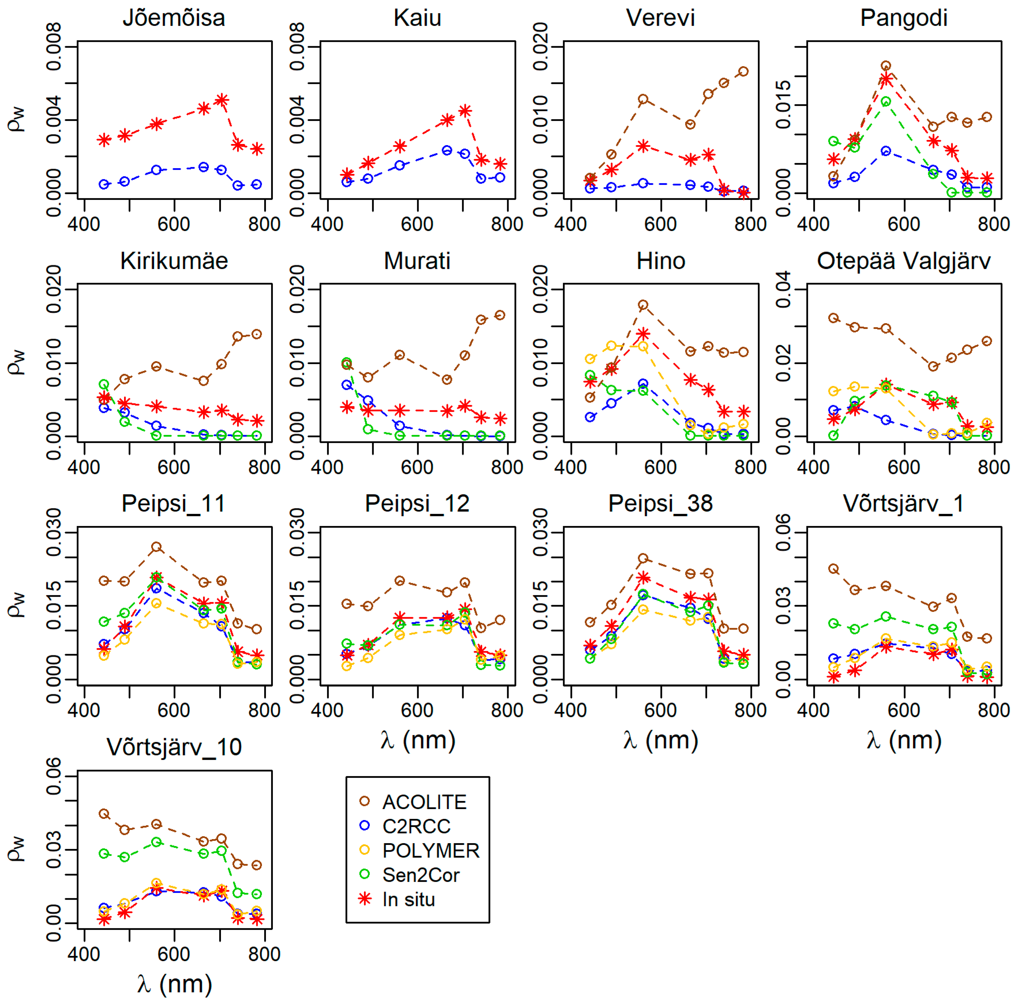
Figure 3 shows the comparison of in situ measured ρw compared to derived ρw from various AC procedures after processor-based flagging. Least retrievals are over highly absorbing small inland lakes (Jõemõisa, Kaiu). Results are better for points further away from the shore waters (e.g., Peipsi_11). Missing ρw specific AC processor spectrum means no results from the AC processor.
In the next paragraph, the results from Figure 3 are explained and linked with the lake’s specification based on the S2 MSI overpass.
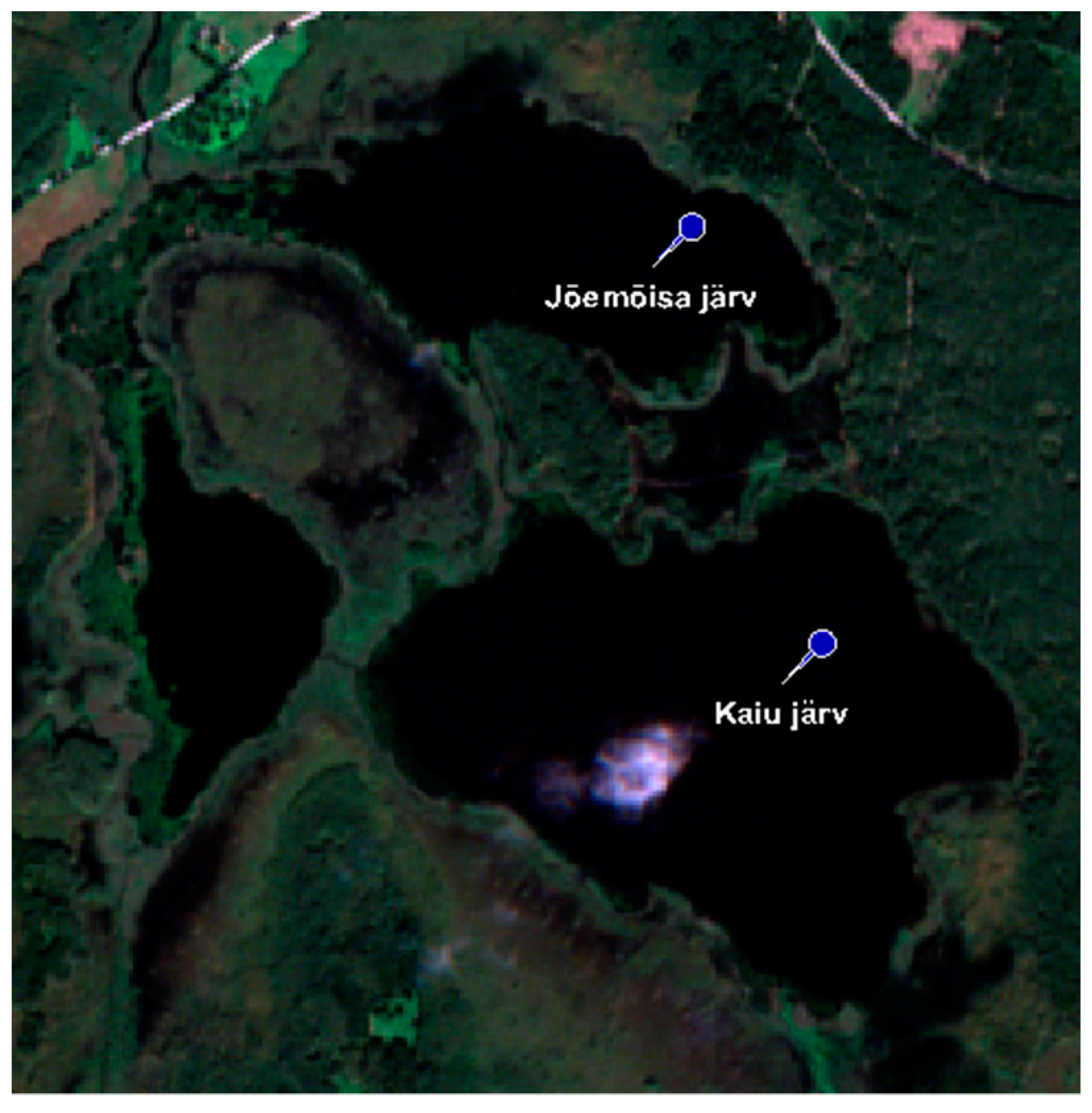
3.1.1. Jõemõisa, Kaiu, Verevi and Pangodi
The S2 MSI images over four small lakes Jõemõisa (Figure A1), Kaiu (Figure A1), Verevi (Figure A2) and Pangodi (Figure A3) originate from 28th of August 2016, and the fieldwork was performed on 25th of August 2016. Both Jõemõisa and Kaiu are classified as Type 2 (non-stratified, color dark/light) waters according to the WFD (Table 1). These two lakes used to be one big lake centuries ago, but because of decreasing water level, they have become separate lakes. Both lakes are eutrophic with high chl a (>21 mg/m3) and very high acdom (442) (>10 m−1) (Table 3), due to the location in the bog area, which results in yellow–brown water color with a low transparency (0.8 m) [60,61]. In situ ρw spectrum is relatively low with a distinctive peak in 705 nm due to strong absorption of CDOM and high chl a. From all the AC processors, only C2RCC provided results for these small lakes, because other AC processors did not derive any ρw values from these conditions. The shape of the C2RCC derived ρw is similar to in situ measured ρw, but it is underestimated in both lakes and the peak due to high chl a absorption is absent.
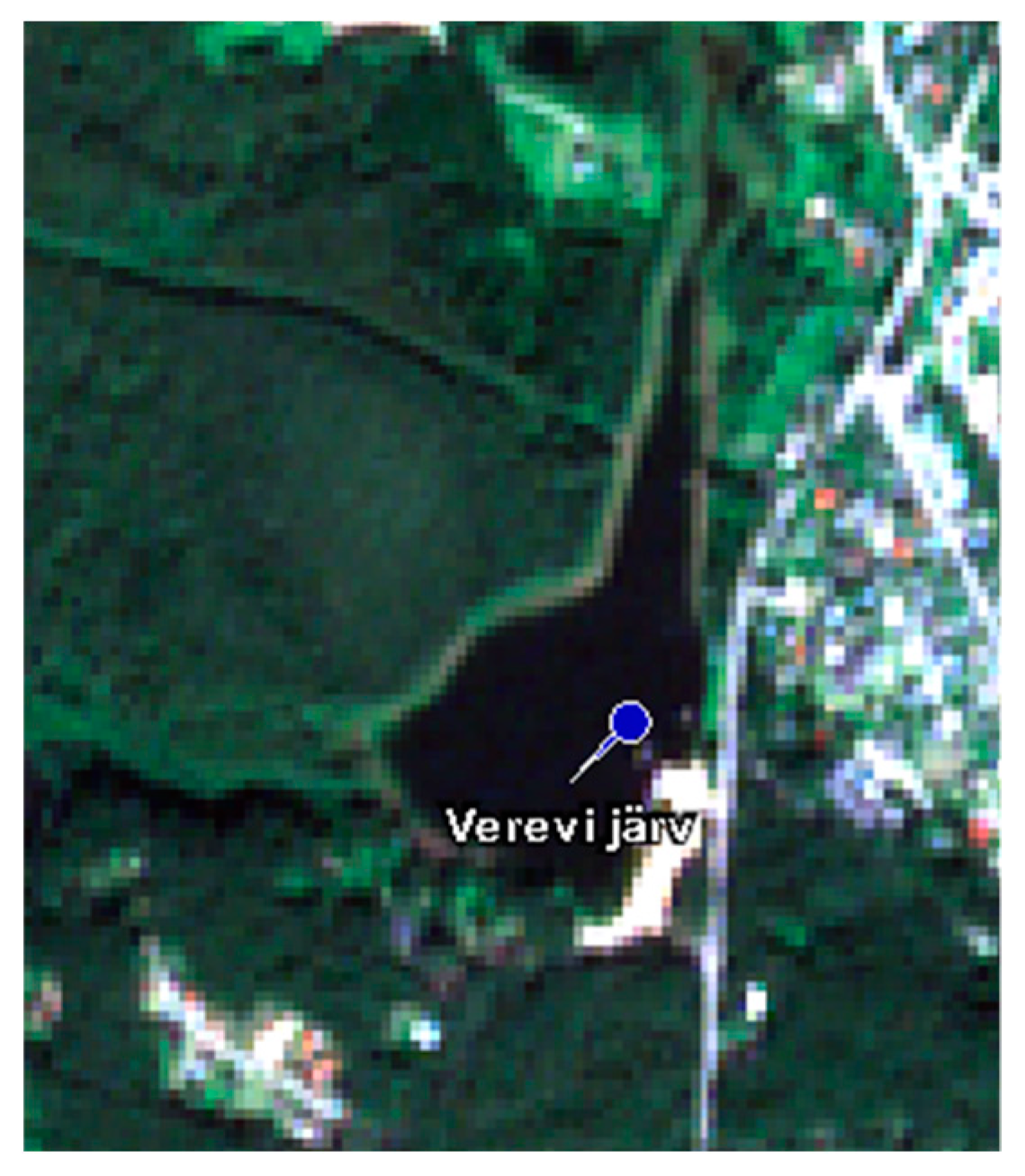
Verevi belongs to Type 3 (stratified, color dark/light) according to the WFD (Table 1). It is a eutrophic lake (chl a 31 mg/m3) with a mostly swampy coastal area, yellow water color, and moderate transparency (1.4 m) (Table 3) [60,61]. C2RCC strongly underestimates in situ measured ρw and does not show the chl a absorption peak at 675 nm (Figure 3). ACOLITE overestimated in situ measured ρw, but shows a similar in situ ρw spectrum chl a absorption peak. NIR bands are really strongly overestimated by ACOLITE, which could be caused by the adjacency effect. Problems with other AC processors could similarly be caused by the adjacency effect, which influences pixels near the coastline. In addition, high CDOM absorption could be the second reason, because, for pixels with a low backscattered light level, the processors are not able to derive ρw.
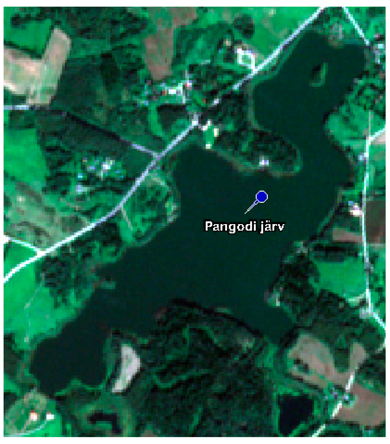
Pangodi (WFD Type 3) is located in between agricultural and forestry areas in the south-east of Estonia, where spring waters are very important sources for nutrient-rich inflow water. Pangodi is a eutrophic lake with moderate chl a (15.2 mg/m3) and relatively low TSM (4.2 mg/m3), and acdom (442) (1.3 m−1) (Table 3). The color of water is yellow–green or green–yellow with low to moderate transparency (1.7 m) [60,61]. Compared to previous lakes, the in situ measured ρw is higher in Pangodi (Figure 3), because of a lower amount of chl a and CDOM. The lower absorption by OAS and the larger water surface area could be the reason that C2RCC, Sen2Cor, and ACOLITE gave similar results as well. The shape of the ρw spectrums of all three AC processors are similar to in situ measured ρw spectrum, but it is underestimated by C2RCC and Sen2Cor and the chl a absorption peak at 675 nm is not derived. ACOLITE estimated the in situ measured ρw very accurately in blue and green wavelengths, but strongly overestimate at NIR wavelengths, similarly to Verevi spectrum. POLYMER did not derive any ρw values from Pangodi.
3.1.2. Kirikumäe, Murati and Hino
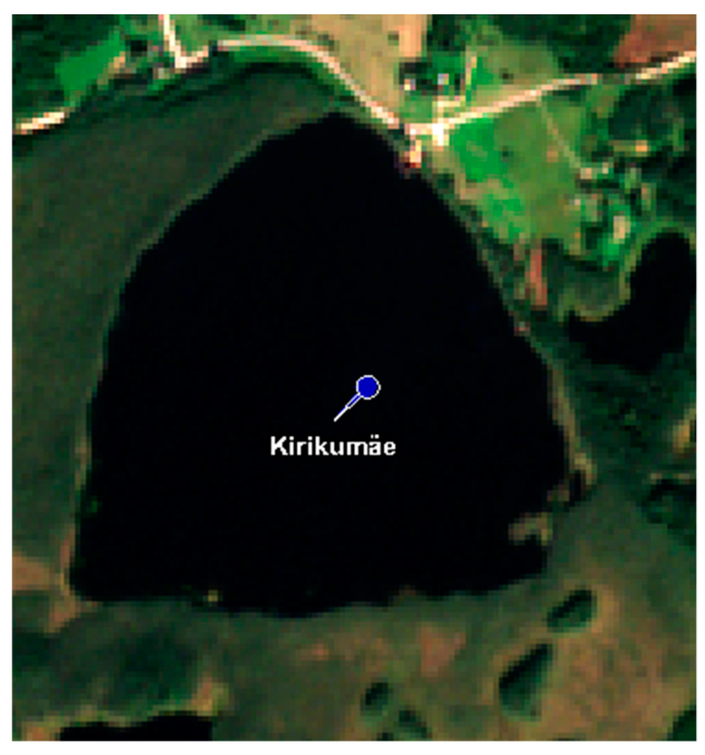
There was a same day match-up for the 30th of August 2017 for Kirikumäe (Figure A4), Murati (Figure A5), and Hino (Figure A6) lakes. These lakes are classified as Type 5 (non-stratified, water color light), Type 3 (stratified, water color dark/light), and Type 2 (non-stratified, water color dark/light) (Table 1), respectively, according to WFD. Kirikumäe is surrounded by a low and swampy areas, which makes it a rare non-stratified eutrophic semi-humus lake, where concentrations of OAS are high (Table 3). The color of the water is yellow to brown–yellow with a low to moderate transparency. Murati is a narrow yellow colored lake, surrounded by agricultural clay soil and sand soil forestry areas. The lake is eutrophic, (chl a > 20 mg/m3) with acdom (442) over 10 m−1 (Table 3), which makes the transparency of the water low [60,61]. Due to the high CDOM absorption, in situ measured ρw is low, which agrees with a low ρw values by C2RCC and Sen2Cor (Figure 3). Although both AC processors derive the ρw with similar shape to in situ data, they slightly overestimate blue part and underestimate green–red part of the in situ measured ρw spectrum and do not derive the chl a absorption peak. ACOLITE overestimates the in situ measured ρw spectrum, except at wavelength 443 and the shape of the ρw is not similar to in situ measured spectrum. NIR bands are strongly overestimated, which has been seen as a problem previously. It can be observed that POLYMER is not able to derive ρw for high chl a and CDOM dominated waters with a small surface area.
Hino has a large surface area and is located between forest areas. The amount of OAS is relatively low (Table 3), except for high TSM (10.7 mg/m3). However, the water of Hino is described as transparent and water color light to yellow–green [60,61]. As TSM is high, the in situ measured ρw spectrum is higher than in previous lakes. The larger surface area and low OAS gave opportunity to derive results besides ACOLITE, C2RCC, and Sen2Cor, from POLYMER, which estimates the ρw at 560 nm similar to the in situ measured ρw (Figure 3) although the blue part is overestimated and red part underestimated. The most similar shape to the in situ measured ρw spectrum are C2RCC and ACOLITE, but C2RCC strongly underestimates in situ ρw similar to Sen2Cor and ACOLITE overestimates, except the blue bands.
3.1.3. Otepää Valgjärv
There was a same day match-up for the 28th of August 2017 for Otepää Valgjärv (Figure A7). It is classified as Type 2 (non-stratified, color dark/light) based on the WFD (Table 1). This green–yellow colored lake is surrounded by forest areas on one side and agricultural areas on the other. It is a eutrophic lake, where chl a is above 25 mg/m3, and TSM is also over 25 mg/m3 (Table 3), which makes the lake’s transparency low [60,61]. The in situ measured ρw shows a strong absorption peak at 675 nm (Figure 3), which is not detected by any of the AC processors, except ACOLITE, but the rest of the ρw spectrum is strongly overestimated. The most similar shape of ρw is Sen2Cor, which estimates the ρw well at 560 nm similar to POLYMER. Although, Sen2Cor is not able to detect chl a absorption at 675 nm, it does not underestimate in situ measured ρw as strongly as C2RCC and POLYMER.
3.1.4. Peipsi
There was a same day match-up for Estonia’s biggest lake Peipsi (Figure A8) from the 14th of September 2016, which belongs to Type 7 (non-stratified, water color light) (Table 1) according to the WFD. The concentrations of chl a (24–35 mg/m3) and TSM (10–16 mg/m3) are high (Table 3). The color of water is yellow–green or green–yellow, and the transparency is moderate (0.6–0.9 m) in the open part of the lake [60,61]. In situ points are located in different parts of the lake: Point Peipsi_11 is located in the middle of the lake, point Peipsi_12 in adjacent to land, and Peipsi_38 is in the mouth of river inflow. AC processors worked well, and the derived values and shapes of the ρw are comparable with in situ data for all points (Figure 3), except for ACOLITE where the ρw values at bands 443 nm, 490 nm, 740 nm, and 783 nm were too high. C2RCC provided no chl a absorption peak. Other AC processors derived a chl a absorption peak at 675 nm. In the river mouth (Peipsi_38) POLYMER was not able to derive ρw in the conditions.
3.1.5. Võrtsjärv
There was also a same day match-up for the 20th of May 2016 for Estonia’s second largest lake Võrtsjärv (Figure A9), which belongs to Type 6 (non-stratified, water color light) according to the WFD (Table 1). Lake Võrtsjärv is a shallow eutrophic lake with high chl a and TSM (Table 3), which causes low water transparency. The color of the water is yellow–green or green–yellow and is caused by a high amount of plankton and resuspension from sediment [60,61]. Point Võrtsjärv_1 is located in the middle of the lake, and point Võrtsjärv_10 is near the coast. While each processor derives the shape of the ρw spectrums similar to in situ data, ACOLITE and Sen2Cor strongly overestimate blue part of the ρw spectrum. As these match-up points were in the vicinity of clouds, ACOLITE and Sen2Cor could be more sensitive to cloud pixels, and this results in a higher ρw. A high TSM (10.8 mg/m3) cause higher ρw at red/NIR wavelengths, which is shown by the results of all AC processors. The chl a absorption peak near 675 nm is derived by all processors except C2RCC.
3.1.6. Comparison of AC processors
Comparison of AC processors over optically different water types revealed that the adjacency effect could cause problems with estimating correct and accurate ρw spectrum in small lakes. Additionally to the adjacency effect, AC processors fail in CDOM dominated waters more frequently, because of high absorption of light in these conditions, which cause lower reflectances. It means that AC processors are not able to retrieve ρw from these kinds of lakes. This has been reported by Grendaité et al. [25] on eutrophic lakes in Lithuania and Kutser et al. [62] in CDOM-dominated waters in Estonia and Sweden. However, C2RCC is capable of deriving ρw in most cases and especially in problematic CDOM dominated waters, where other AC processors failed. C2RCC is able to work in cases of different water types. Sen2Cor and ACOLITE are similarly able to work in CDOM dominated waters, although they do not derive ρw more often than C2RCC. ACOLITE typically overestimates, similar to Sen2Cor’s, the blue part of the ρw spectrum. Caballero et al. [63] have studied Spanish coastal areas, applying ACOLITE and POLYMER on medium to highly turbid waters and found that ACOLITE similarly overestimated the blue part of the spectrum and the same has been noticed by Dörnhöfer et al. [64] on oligotrophic lakes. Additionally, ACOLITE often overestimates NIR wavelengths, which could be caused by the adjacency effect. Caballero et al. [63] observed similar results as shown in this study for POLYMER which gave accurate results to in situ measurements in TSM dominated waters, such as coastal areas. Results of comparison of all AC processors are summarized in the Table 4.
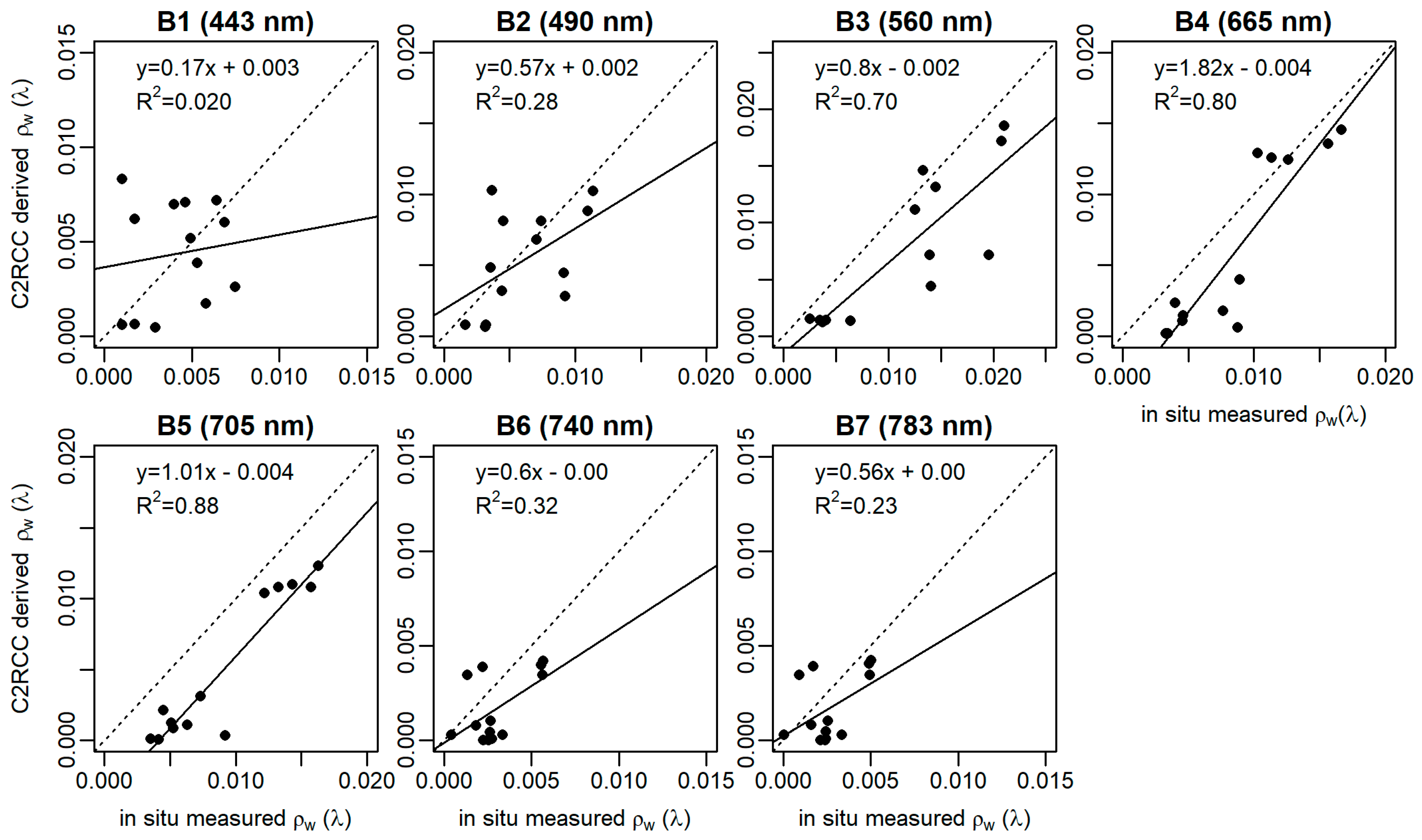
The number of pixels for comparison among AC processors was the highest for C2RCC (N = 13), which gives the opportunity to obtain information from small lakes. The least data were retrieved with POLYMER (N = 7) because it did not retrieve ρw in small lakes. The coefficient of determination shows the highest correlation in all AC processors at the wavelengths 560, 665, and 705 nm, which are the main wavelengths for developing chl a algorithms for optically complex Case 2 waters. C2RCC shows the highest correlation (R2 > 0.7) at these wavelengths, whereas the correlation is smaller (R2 < 0.7) for other AC processors. Zero I for C2RCC indicates that derived ρw fit well with the in situ measured ρw. ACOLITE gives higher I values (I ≥ 0.1) and other AC lower I values (I ≤ 0.0). S near to one indicates a good fit between derived in situ measured ρw. At the main wavelengths of developing chl a algorithms, the S was close to one for the C2RCC processor (S = 0.8–1.18).
Based on the average absolute percentage difference values, POLYMER gives the most accurate results compared to the in situ measured ρw at the main chl a developing wavelengths (ψ < 40.6). According to the root–mean–square difference, C2RCC and POLYMER show the most accurate results, which means that C2RCC and POLYMER derived ρw is the most comparable with in situ measured ρw, C2RCC was Δ = 0.01 only at 560 nm. Otherwise it was 0. As bias indicates over- or underestimation, then AC processors rather underestimate the in situ measured ρw spectrum.
Based on the derived statistics, C2RCC and POLYMER showed the highest accuracy. As the purpose of the study is to estimate water quality in small lakes, the high number of derived water pixels is an essential value, which is highest in the case of C2RCC. The reason for the highest number of derived results in case of C2RCC is the processor-based flagging. It did not flag out as many pixels as ACOLITE, POLYMER, and Sen2Cor in optically complex waters. Based on the coefficient of determination and root–mean–square difference, the C2RCC was selected as a processor to derive the ρw as an input for chl a algorithms. Figure 4 shows the correlation between derived ρw of C2RCC and in situ measured ρw at given wavelengths. Values of derived ρw of C2RCC are rather underestimated compared with in situ measured ρw values. Table 4 supports the underestimation evidence because the bias is negative from 490 nm to 740 nm.
3.2. Comparing and Developing chl a Algorithms for S2 MSI
Based on the literature overview, 28 empirical algorithms were selected that could be adapted to S2 MSI bands (Table 5). These algorithms were tested on GLaSS dataset, where oligotrophic to hyper eutrophic lakes were represented.
To analyze the applicability of various empirical approaches on different lakes, algorithms (Table 5) were applied either on L1C S2 MSI data or on in situ measured ρw data (GLaSS dataset) to derive the conversion factors for estimating chl a. On L1C data, various MCI-based approaches were tested (Table 6). This analysis is based on a limited number of data (Table 3, N = 12) with relatively high scatter in the data (R2 ~ 0.25) As there are only a few match-ups between S2 MSI, and in situ data, the GLaSS dataset was used to test the algorithms (Table 5) on different water types and derive the conversion factors suitable for S2 L2 data for estimating chl a (Table 6) For every water type (or lake), the three best empirical approaches were chosen based on the highest R2 values (Table 6).
The highest correlation between tested empirical approaches and corresponding chl a were retrieved in Võrtsjärv and Vesijärvi, which gave R2 > 0.92 and R2 > 0.94, respectively. Two-Band NIR–Red Model algorithms work better in low CDOM waters (acdom (442) < 4.1 m−1). The band ratio model based on R705/R665 works for eutrophic (e.g., Vesijärv (R2 = 0.97)) to oligotrophic (e.g., Garda (R2 = 0.2)) waters. As Three-Band NIR–Red Model-based algorithms are working for turbid waters, good correlation is shown for the band ratio algorithm (R665−1 − R705−1) × R740 for Võrtsjärv (R2 = 0.92). A high correlation is shown for the same band ratio algorithm using band R783 instead of R740 in Võrtsjärv (R2 = 0.93). Four-Band NIR–Red Model algorithms show good results in high TSM concentration waters like Peipsi (R2 = 0.4) and Võrtsjärv (R2 = 0.92). In Maggiore, where concentrations of OAS are low, the Blue–Green Two-Band Ratio Model is working (e.g., R490/R443 (R2 = 0.31)). However, for optically complex oligotrophic lakes (e.g., Maggiore and Garda) the proposed empirical algorithms are not optimal, and the approaches based on bio-optical modelling derive more accurate results [24]. The MCI derived algorithm (index 0.53 and 0.339, depending on S2 band, respectively, R740 or R783) shows good correlation in Finnish boreal lakes (R2 > 0.6) and the Betuwe area (R2 = 0.76), which has relatively different water types based on the chl a (Betuwe, chl a median = 23.5 mg/m3 and Finnish boreal lakes, chl a median = 3.2 mg/m3) and TSM (Betuwe, TSM max = 28.2 mg/m3 and Finnish boreal lakes, TSM max = 2.1 mg/m3). However, applying the MCI algorithm on L1C data of Estonian lakes (chl a = 15.2–34.8 mg/m3, acdom (442) = 1.3–14 m−1) correlation was low (R2 = 0.25–0.26).
3.2.1. Spatial Analysis of C2RCC Derived ρw Product over Mesotrophic and Eutrophic Lakes
Applying C2RCC on various S2 MSI data over eutrophic lakes revealed that in the case of smaller lakes, especially with a sophisticated shoreline, the C2RCC often produced invalid ρw—highest value at the blue band and constantly decreasing towards longer wavelengths (Figure 5b, red line). This was not in agreement with in situ measured values (Figure 5b, grey line). An example of C2RCC ρw product in two eutrophic lakes, a narrow lake Raigastvere (Figure 5a) and larger Saadjärv (Figure 5c), show that the invalid spectrum (red area) is often derived near the coastal area. Raigastvere’s surface area is 11 ha (chl a 13.8 mg/m3, TSM 5.7 mg/m3, acdom (442) 3.2 m−1, Sechhi 1 m, average depth 3.2 m) and the lake is 510 m wide, while Saadjärv is 708 ha large (chl a 3.9 mg/m3, TSM 2 mg/m3, acdom (442) 0.9 m−1, Sechhi 4 m, average depth 8 m) and 1.8 km wide and both lakes are classified as eutrophic lakes [60]. Due to low transparency in these lakes, the invalid spectrum is not produced by bottom reflection but could be due to the adjacency effect, where vegetation is influencing water pixels. On the other hand, Martins et al. [72] have pointed out the adjacency problem while applying ACOLITE and Sen2Cor AC processors on complex Amazon floodplain lakes, where forest adjacency effect increased ρw in longer wavelengths. A similar tendency was noted by Dörnhöfer et al. [64] on oligotrophic lakes. The majority of the pixels are invalid at the end of the June (29 June2016) when there was a high peak of phytoplankton growth in the surface water. C2RCC quality flags were not sensitive to these invalid pixels. Therefore, for further study, condition band 3 (560 nm) < band 1 (443 nm) were applied to C2RCC images to flag out invalid pixels. The condition was often true in small very sophisticated mesotrophic and eutrophic lakes.
3.2.2. Ecological Status of Water in Lakes Based on chl a
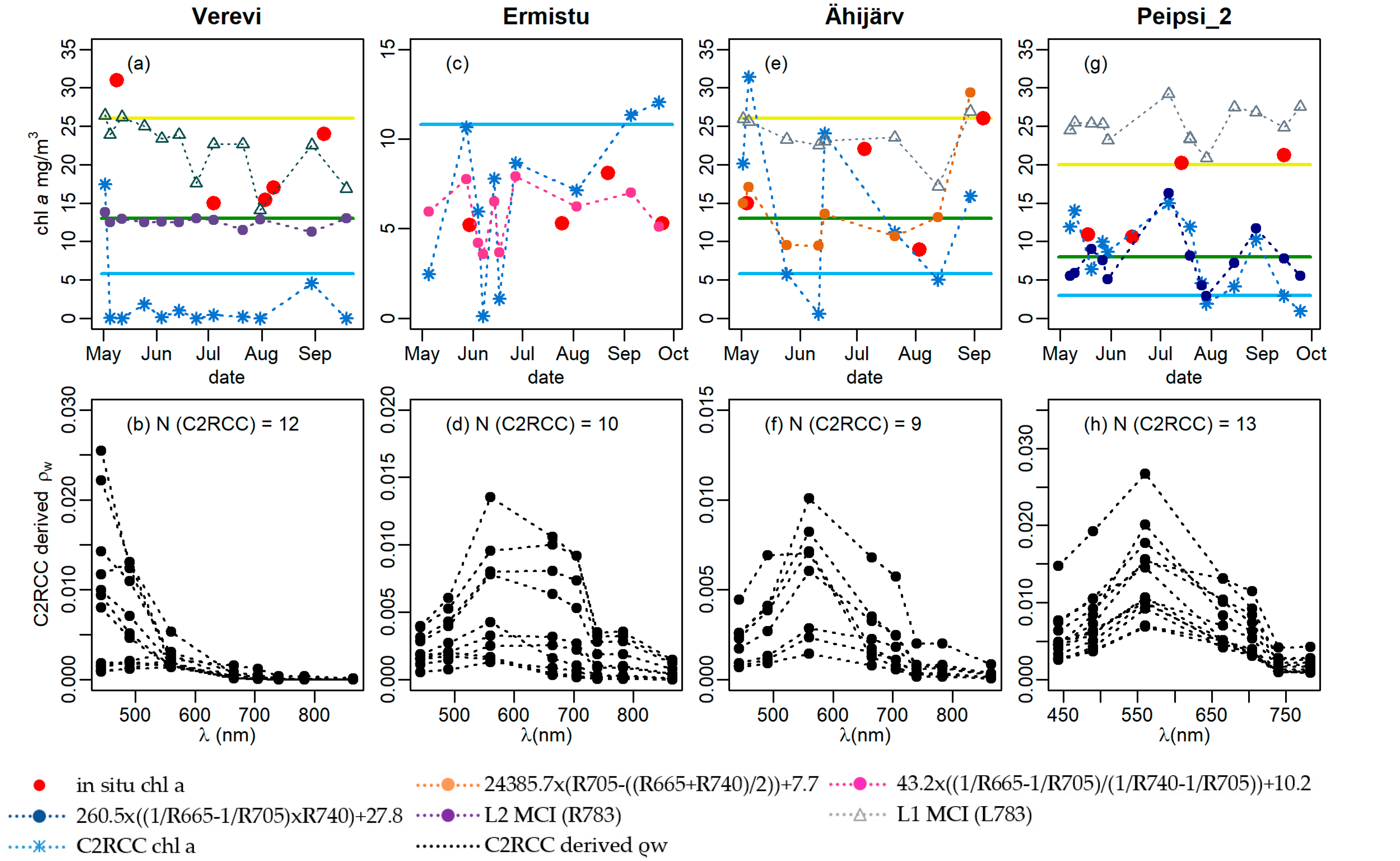
For estimating the ecological status of a water body based on chl a, the specific thresholds have to be considered for each lake type according to WFD (Table 2). Figure 6 represents the seasonal dynamics of chl a and the corresponding ecological status class, focusing on different types of water according to WFD using empirical algorithms from Table 6. Additionally, the chl a value as output from C2RCC standard algorithm is shown on the Figure 6.
As Verevi is a small lake, invalid ρw spectrums are shown in Figure 6b as described previously in Figure 5b. Applying chl a algorithms on Verevi, the concentration of chl a remains constant (Figure 6a), because the Case 2 ρw spectrums are not typical. However, the MCI algorithm was applied to L1C data, which derives accurate results compared to in situ data and shows seasonal dynamics. Lakes with a larger water surface area show better results using C2RCC ρw. Ermistu belongs to type 2 (non-stratified, water color dark/light), with chl a concentration between 10.8–28 mg/m3 and assigned “good” status class. Four-Band NIR–Red Model chl a = 43.2 × (R665−1 − R705−1)/(R740−1 − R705−1) + 10.2 approach worked best and showed a similar trend with in situ measured chl a. The standard C2RCC algorithm estimates chl a similar to empirical algorithms, but the range of minimum and maximum values are higher and makes it less stable for estimating chl a (Figure 6c). As the water surface is large (ha = 450 ha), the ρw of C2RCC was estimated well, because the adjacency effect did not influence the water pixels of the lake. Both in situ measured and empirical approach derived chl a values are low (chl a < 10 mg/m3) and there is no strong chl a absorption peak at 675 nm in the C2RCC derived ρw spectrums (Figure 6d), which is reflected in the stable seasonal dynamics. The ecological water status in Ermistu was estimated “very good” both by in situ measurements (average in situ chl a 6.0 mg/m3, N = 4) and by satellite-derived chl a (average 5.7 mg/m3, N = 10).
Ähijärv belongs to Type 3 (stratified, water color dark/light), therefore, chl a between 5.8–13 mg/m3 assigns the lake into “good” ecological status by class. Algorithm chl a = 24385.4 × (R705 − ((R665 + R740)/2)) + 7.7 gives the most accurate results for this large lake. The same band ratio has been used by Toming et al. [69] on lakes with chl a in range 3–72 mg/m3 retrieving R2 = 0.8. An MCI based approach gave similar concentrations to in situ measurements. However lower chl a values were overestimated. Futhermore, in other investigated Type 3 lakes, MCI based algorithm for ρw, estimates chl a in the same order as in situ measured values. The standard CR2CC algorithm gave very low or very high concentrations, which has been noted previously, but the dynamics remain similar to in situ measurements. ρw of Ähijärv showed slight chl a absorption (Figure 6f), but not as strong as it should be with chl a over 20 mg/m3. The ecological water status in Ähijärv was estimated as “moderate” by in situ measurements (average in situ chl a 18.0 mg/m3, N = 4) as well as satellite-derived chl a (average empirical algorithm 14.7 and 16.4 mg/m3, N = 9) and by L1C MCI (23.6 mg/m3, N = 9).
Peipsi 2 belongs to Type 6 (described previously). The chl a between 3–8 mg/m3 assigns the lake into “good” ecological status. Three-Band NIR–Red Model algorithm chl a = 260.1 × ((R665−1 − R705−1) × R740) + 27.9, with different coefficients compared to Type 2 lakes, gave similar dynamics for chl a compared to in situ measurements, although similar to C2RCC with an underestimation of values. The MCI algorithm applied to L1C data overestimates the chl a, because chl a concentration is lower than 15 mg/m3 at the beginning of summer (Figure 6g). However, it follows similar dynamics as in situ chl a and with higher concentrations. Since Peipsi is a larger lake, water pixels were not affected as much as for small lakes by the coastline, which shown by the number of suitable C2RCC pixels (N = 13). The ecological water status in Peipsi_2 was estimated as “moderate” by in situ measurements (average in situ chl a 16.8 mg/m3, N = 5), “good” and “moderate” by satellite-derived chl a (average 7.4 and 16.7 mg/m3, N = 13) and “bad” by L1C MCI (25 mg/m3, N = 13).
It was possible to estimate the ecological status of water by chl a in some cases. Bresciani et al. [24] have investigated subalpine lakes with S2 MSI and Landsat OLI, which showed a good advantage for spatial scale analyses over in situ measurements. In situ monitoring for chl a includes point measurements from the lakes, but remote sensing is capable of estimating chl a values over the lake. High revisitation with the two satellites helps to detect intense phytoplankton blooms and estimate the ecological status of water considering phytoplankton events in the final classification. The possibility of estimating chl a depended on the capability of C2RCC to derive accurate ρw in small lakes and in the vicinity of land. In Type 2, algorithm (R665−1 − R705−1)/(R740−1 − R705−1) worked well, giving similar results as in situ measurements. Three-Band NIR–Red Model algorithm R705 − ((R665 + R740)/2), also worked in Peipsi and smaller lakes. However, the standard C2RCC algorithm typically estimates chl a reasonably well, when chl a < 10 mg/m3. The MCI based approach L2 MCI (R783) applied on ρw, worked in Ähijärv and Peipsi_2. The L1C MCI approach typically overestimated in situ measured chl a, but showed similar dynamics and concentrations when chl a > 15 mg/m3. The MCI algorithm applied on L1C data is the best solution for avoiding failures which come from AC or in the case of intense phytoplankton blooms. The same tendency has been shown by Toming et al. [69], Grendaite et al. [25], and Alikas et al. [73], when band ratio algorithms applied on L1C data gave higher accuracy in deriving chl a compared to L2 data. However, more available data is needed to investigate relationship between MCI and chl a. The accuracy in the final chl a product could also be increased by using bands with higher spatial resolution (10 m, 20 m) which could decrease error propagation due to the adjacency effect.
4. Conclusions
The EU WFD obligates member states to monitor lakes larger than 50 ha and derive their ecological status. The goal is to achieve, at least, “good” ecological status and take measures to improve the status, if needed. S2 MSI has suitable spatial resolution from 10 m, which could support the development of new applications over lakes for fulfilling WFD monitoring requirements. With both satellites, S2A and S2B, the temporal resolution of 2 to 3 days provides the possibility to include and analyze more data for testing and for developing new applications for S2 MSI satellites. Even more, it has the advantage of providing time series and dynamics of chl a in lakes.
S2 MSI is mainly designed for vegetation applications, therefore, it is important to compare different AC processors for finding the most suitable for water applications. As the AC procedure is an essential tool for developing chl a algorithms, four different AC processors: ACOLITE, C2RCC, POLYMER, and Sen2Cor were tested in this study. Based on the 13 match-up points, C2RCC was chosen due to the high correlation with in situ measurements at bands useable for deriving chl a.
As chl a is one of the main parameters for estimating the ecological status of water based on WFD, the second part of the study included testing and developing chl a algorithms adjusted to S2 MSI bands. Further investigation showed that C2RCC is not able to give accurate results in small, narrow lakes, where the adjacency effect affects the pixels near the coastline. Therefore, it is important to develop corrections for the adjacency effect, which could help avoid invalid mixed pixels in analyses.
In some cases, where the adjacency effect was smaller, especially in larger lakes (over 90 ha) and where the shape of the lake is round, it was possible to estimate chl a in water surface using empirical algorithms. The standard C2RCC chl a algorithm constantly estimates the value of chl a either higher or lower, compared to in situ data, but with similar seasonal dynamics. In case of high chl a (up to 150 mg/m3), good agreement with in situ data was derived with Three-Band NIR–Red Model (R665−1 − R705−1) × R740 and R705 − ((R665 + R740)/2) algorithm. In the lakes with high TSM (up to 19 mg/m3), Four-Band NIR–Red model algorithm (R665−1 − R705−1)/(R740−1 − R705−1) worked best, removing the TSM influence, and as previously mentioned, the Three-Band NIR–Red Model algorithm and MCI algorithm applied on L1C data estimated chl a similar to in situ measurements in case of chl a > 15 mg/m3. As not influenced by ACs, the MCI algorithm is the most suitable on S2 L1C data, however, further investigation is needed.
Furthermore, the C2RCC processor was not very sensitive in estimating chl a absorption at band 665 nm, which could be due to the adjacency effect in small lakes. It means that more validation data from optically complex waters are essential for improving AC processors. S2 MSI has potential for deriving water quality parameters from small lakes for fulfilling EU WFD monitoring and reporting requirements. However, improvements of ACs algorithms are essential for producing higher-level water quality products. This would allow to use S2 MSI advantages over in situ measurements and support the regular monitoring over small lakes.
Author Contributions
A.A. and K.A. are responsible for conceptualization and methodology. A.A. did the data analyzing, writing the first draft and visualization. Both A.A. and K.A. collected some of the in situ data and contributed to the final version of the manuscript.
Funding
This research was funded by European Union’s Horizon 2020 research and innovation program grant number 730066 and by the Estonian Research Council grant (PSG10).
Acknowledgments
We are grateful to four anonymous reviewers for their feedback and suggestions that helped to improve the manuscript. We would like to thank you people from Centre for Limnology providing in situ data and water remote sensing workgroup (Martin Ligi, Ilmar Ansko, Kersti Kangro, Kristi Uudeberg, Mirjam Randla, Getter Põru) from Tartu Observatory performing fieldworks (collecting radiometric data and analyzing water samples). We are very grateful to FP 7 project GLaSS (313256) colleagues Claudia Giardino, Mariano Bresciani (Consiglio Nazionale delle Ricerche), Sampsa Koponen, Kari Kalio (Suomen Ymparistokeskus), Yunlin Zhang (Nanjing Institute of Geography and Limnology, Chinese Academy of Sciences), Annelies Hommersom (Water Insight) for the contribution to bio-optical dataset used to test the empirical algorithms over various optical water types.
Conflicts of Interest
The authors declare no conflict of interest.
Appendix A
Figure A1.
S2 MSI image of Jõemõisa and Kaiu from 28th of August 2016.

Figure A2.
S2 MSI image of Verevi from 28th of August 2016.

Figure A3.
S2 MSI image of Pangodi from 28th of August 2016.

Figure A4.
S2 MSI image of Kirikumäe from 30th of August 2017.

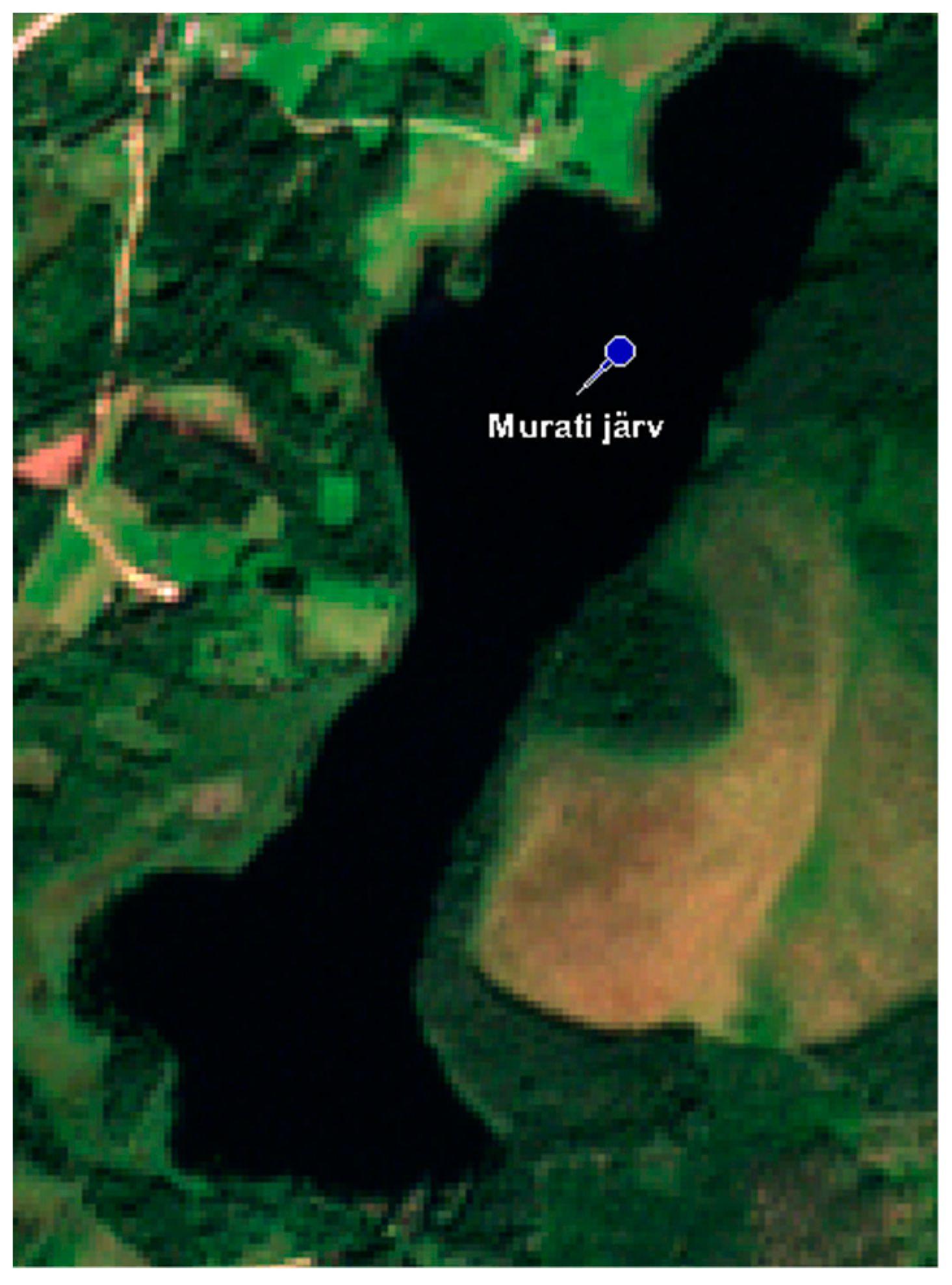
Figure A5.
S2 MSI image of Murati from 30th of August 2017.

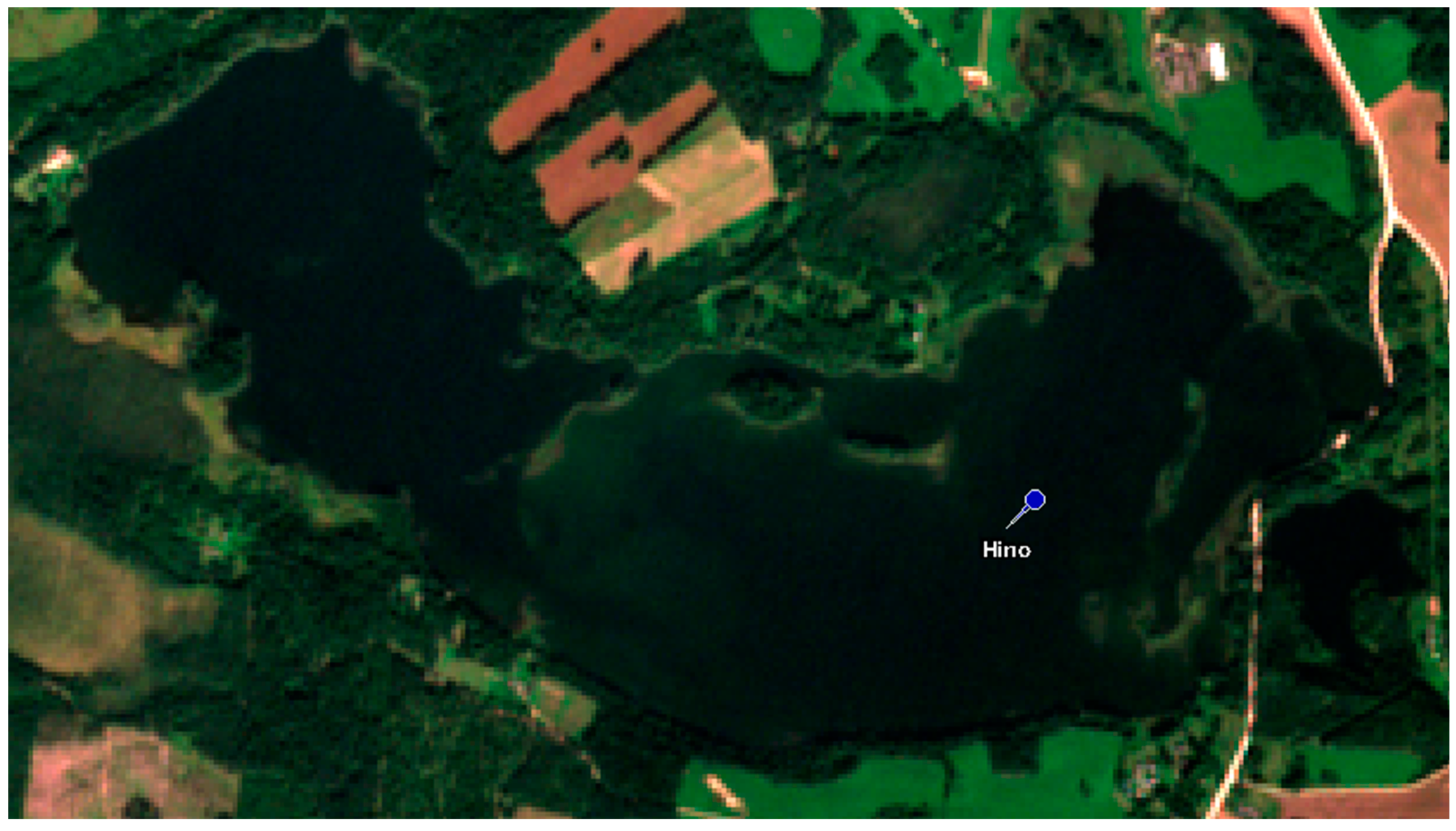
Figure A6.
S2 MSI image of Hino from 30th of August 2017.

Figure A7.
S2 MSI image of Otepää Valgjärv from 28th of August 2017.

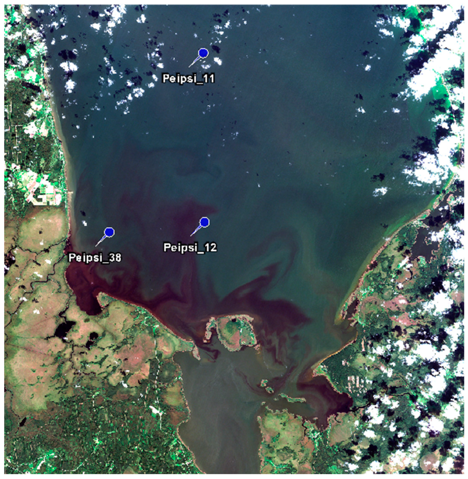
Figure A8.
S2 MSI image of Peipsi from 14th of September 2016.

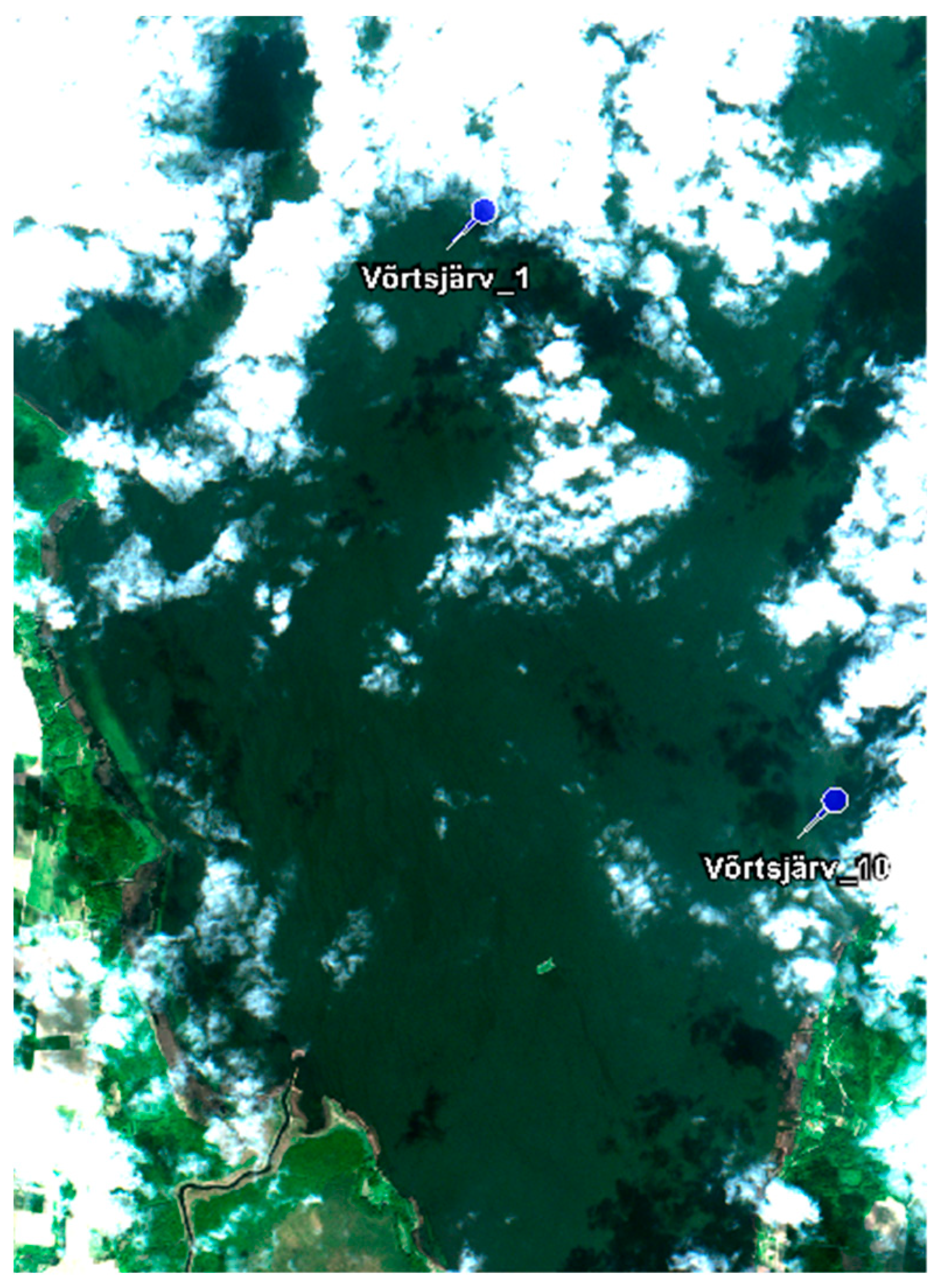
Figure A9.
S2 MSI image of Võrtsjärv from 20th of May 2016.

References
- The European Parliament, the Council of the European Union. WFD Directive 2000/60/EC of the European Parliament and of the Council of 23 October 2000 establishing a framework for Community action in the field of water policy. Off. J. Eur. Parliam. 2000, 327, 1–73. [Google Scholar] [CrossRef]
- EU Water Directors. Common Implementation Strategy for the Water Framework Directive and the Floods Directive, WFD Reporting Guidance 2016; EU: Brussels, Belgium, 2016. [Google Scholar]
- Ferreira, J.G.; Vale, C.; Soares, C.V.; Salas, F.; Stacey, P.E.; Bricker, S.B.; Silva, M.C.; Marques, J.C. Monitoring of coastal and transitional waters under the E.U. water framework directive. Environ. Monit. Assess. 2007, 135, 195–216. [Google Scholar] [CrossRef] [PubMed]
- Ministry of Environment Pinnaveekogumite Moodustamise Kord ja Nende Pinnaveekogumite Nimestik, Mille Seisundiklass Tuleb Määrata, Pinnaveekogumite Seisundiklassid ja Seisundiklassidele Vastavad Kvaliteedinäitajate Väärtused Ning Seisundiklasside Määramise kord-RT I, 25.11.2010. Available online: https://www.riigiteataja.ee/akt/125112010015 (accessed on 3 September 2018).
- Chen, Q.; Zhang, Y.; Hallikainen, M. Water quality monitoring using remote sensing in support of the EU water framework directive (WFD): A case study in the Gulf of Finland. Environ. Monit. Assess. 2007, 124, 157–166. [Google Scholar] [CrossRef] [PubMed]
- Matthews, M.W. A current review of empirical procedures of remote sensing in Inland and near-coastal transitional waters. Int. J. Remote Sens. 2011, 32, 6855–6899. [Google Scholar] [CrossRef]
- Salem, S.I.; Strand, M.H.; Higa, H.; Kim, H.; Kazuhiro, K.; Oki, K.; Oki, T. Evaluation of meris chlorophyll-a retrieval processors in a complex turbid lake kasumigaura over a 10-year mission. Remote Sens. 2017, 9, 1022. [Google Scholar] [CrossRef]
- Chen, Q.; Zhang, Y.; Ekroos, A.; Hallikainen, M. The role of remote sensing technology in the EU water framework directive (WFD). Environ. Sci. Polic. 2004, 7, 267–276. [Google Scholar] [CrossRef]
- Salem, S.I.; Higa, H.; Kim, H.; Kobayashi, H.; Oki, K.; Oki, T. Assessment of chlorophyll-a algorithms considering different trophic statuses and optimal bands. Sensors (Switzerland) 2017, 17, 1746. [Google Scholar] [CrossRef] [PubMed]
- Lins, R.C.; Martinez, J.M.; Marques, D.D.; Cirilo, J.A.; Fragoso, C.R. Assessment of chlorophyll-a remote sensing algorithms in a productive tropical estuarine-lagoon system. Remote Sens. 2017, 9, 516. [Google Scholar] [CrossRef]
- Werdell, P.J.; McKinna, L.I.W.; Boss, E.; Ackleson, S.G.; Craig, S.E.; Gregg, W.W.; Lee, Z.; Maritorena, S.; Roesler, C.S.; Rousseaux, C.S.; et al. An overview of approaches and challenges for retrieving marine inherent optical properties from ocean color remote sensing. Prog. Oceanogr. 2018, 160, 186–212. [Google Scholar] [CrossRef]
- Duan, H.; Zhang, Y.; Zhang, B.; Song, K.; Wang, Z. Assessment of chlorophyll-a concentration and trophic state for lake chagan using landsat TM and field spectral data. Environ. Monit. Assess. 2007, 129, 295–308. [Google Scholar] [CrossRef]
- Moses, W.J.; Gitelson, A.A.; Berdnikov, S.; Povazhnyy, V. Estimation of chlorophyll-a concentration in case II waters using MODIS and MERIS data—Successes and challenges. Environ. Res. Lett. 2009, 4. [Google Scholar] [CrossRef]
- Wozniak, M.; Bradtke, K.M.; Krezel, A. Comparison of satellite chlorophyll a algorithms for the Baltic Sea. J. Appl. Remote Sens. 2014, 8. [Google Scholar] [CrossRef]
- Zhang, Y.; Ma, R.; Duan, H.; Loiselle, S.; Xu, J. A spectral decomposition algorithm for estimating chlorophyll-a concentrations in Lake Taihu, China. Remote Sens. 2014, 6, 5090–5106. [Google Scholar] [CrossRef]
- Carstensen, J.; Klais, R.; Cloern, J.E. Phytoplankton blooms in estuarine and coastal waters: Seasonal patterns and key species. Estuar. Coast. Shelf Sci. 2015, 162, 98–109. [Google Scholar] [CrossRef] [Green Version]
- Zhang, F.; Li, J.; Shen, Q.; Zhang, B.; Wu, C.; Wu, Y.; Wang, G.; Wang, S.; Lu, Z. Algorithms and schemes for chlorophyll a estimation by remote sensing and optical classification for turbid lake Taihu, China. IEEE J. Sel. Top. Appl. Earth Obs. Remote Sens. 2015, 8, 350–364. [Google Scholar] [CrossRef]
- Giardino, C.; Bresciani, M.; Stroppiana, D.; Oggioni, A.; Morabito, G. Optical remote sensing of lakes: An overview on Lake Maggiore. J. Limnol. 2014, 73, 201–214. [Google Scholar] [CrossRef]
- Gohin, F.; Saulquin, B.; Oger-Jeanneret, H.; Lozac’h, L.; Lampert, L.; Lefebvre, A.; Riou, P.; Bruchon, F. Towards a better assessment of the ecological status of coastal waters using satellite-derived chlorophyll-a concentrations. Remote Sens. Environ. 2008, 112, 3329–3340. [Google Scholar] [CrossRef]
- Bresciani, M.; Stroppiana, D.; Odermatt, D.; Morabito, G.; Giardino, C. Assessing remotely sensed chlorophyll-a for the implementation of the Water Framework Directive in European perialpine lakes. Sci. Total Environ. 2011, 409, 3083–3091. [Google Scholar] [CrossRef] [Green Version]
- Alikas, K.; Kangro, K.; Randoja, R.; Philipson, P.; Asuküll, E.; Pisek, J.; Reinart, A. Satellite-based products for monitoring optically complex inland waters in support of EU Water Framework Directive. Int. J. Remote Sens. 2015, 36, 4446–4468. [Google Scholar] [CrossRef]
- Philipson, P.; Eriksso, K.; Stelzer, K. MERIS data for monitoring of small and medium sized humic Swedish lakes. In Proceedings of the Measuring and Modeling of Multi-Scale Interactions in the Marine Environment—IEEE/OES Baltic International Symposium 2014, BALTIC 2014, Tallinn, Estonia, 27–29 May 2014. [Google Scholar]
- Attila, J.; Kauppila, P.; Kallio, K.Y.; Alasalmi, H.; Keto, V.; Bruun, E.; Koponen, S. Applicability of Earth Observation chlorophyll-a data in assessment of water status via MERIS—With implications for the use of OLCI sensors. Remote Sens. Environ. 2018, 212, 273–287. [Google Scholar] [CrossRef]
- Bresciani, M.; Cazzaniga, I.; Austoni, M.; Sforzi, T.; Buzzi, F.; Morabito, G.; Giardino, C. Mapping phytoplankton blooms in deep subalpine lakes from Sentinel-2A and Landsat-8. Hydrobiologia 2018, 824, 197–214. [Google Scholar] [CrossRef] [Green Version]
- Grendaitė, D.; Stonevičius, E. Chlorophyll-a concentration retrieval in eutrophic lakes in Lithuania from Sentinel-2 data. Geol. Geogr. 2018, 4, 15–28. [Google Scholar] [CrossRef]
- Klein, T.; Nilsson, M.; Persson, A.; Håkansson, B. From Open Data to Open Analyses—New Opportunities for Environmental Applications? Environments 2017, 4, 32. [Google Scholar] [CrossRef]
- Morel, A.; Prieur, L. Analysis of variations in ocean color. Limnol. Oceanogr. 1977, 22, 709–722. [Google Scholar] [CrossRef]
- Odermatt, D.; Gitelson, A.; Brando, V.E.; Schaepman, M. Review of constituent retrieval in optically deep and complex waters from satellite imagery. Remote Sens. Environ. 2012, 118, 116–126. [Google Scholar] [CrossRef] [Green Version]
- Hieronymi, M.; Krasemann, H.; Müller, D.; Brockmann, C.; Ruescas, A.; Stelzer, K.; Nechad, B.; Ruddick, K.; Simis, S.; Tilstone, G.; et al. Ocean colour remote sensing of extreme case-2 waters. In Proceedings of the conference held Living Planet Symposium, Prague, Czech Republic, 9–13 May 2016. [Google Scholar]
- Shanmugam, P. CAAS: An atmospheric correction algorithm for the remote sensing of complex waters. Ann. Geophys. 2012, 30, 203–220. [Google Scholar] [CrossRef]
- Moore, G.F.; Aiken, J.; Lavender, S.J. The atmospheric correction of water colour and the quantitative retrieval of suspended particulate matter in Case II waters: Application to MERIS. Int. J. Remote Sens. 1999, 20, 1713–1733. [Google Scholar] [CrossRef]
- IOCCG. Remote Sensing of Ocean Colour in Coastal, and Other Optically-Complex, Waters; Sathyendranath, S., Ed.; Reports of the International Ocean-Colour Coordinating Group, No. 3; IOCCG: Dartmouth, MA, Canada, 2000. [Google Scholar]
- Candiani, G.; Giardino, C.; Brando, V.E. Adjacency effects and bio-optical model regionalisation: Meris data to assess lake water quality in the subalpine ecoregion. In Proceedings of the Envisat Symposium, Montreux, Switzerland, 23–27 April 2007. [Google Scholar]
- Sterckx, S.; Knaeps, E.; Ruddick, K. Detection and correction of adjacency effects in hyperspectral airborne data of coastal and inland waters: The use of the near infrared similarity spectrum. Int. J. Remote Sens. 2011, 32, 6479–6505. [Google Scholar] [CrossRef]
- Fell, F.; Fischer, E.; Schaale, M.; Schroder, T. Retrieval of chlorophyll concentration from MERIS measurements in the spectral range of the sun-induced chlorophyll fluorescence. Proc. SPIE 2003, 4892, 116–123. [Google Scholar] [CrossRef]
- Gitelson, A.A. The peak near 700 nm on radiance spectra of algae and water: Relationships of its magnitude and position with chlorophyll. Int. J. Remote Sens. 1992, 13, 3367–3373. [Google Scholar] [CrossRef]
- Matthews, M.W.; Bernard, S.; Winter, K. Remote sensing of cyanobacteria-dominant algal blooms and water quality parameters in Zeekoevlei, a small hypertrophic lake, using MERIS. Remote Sens. Environ. 2010, 114, 2070–2087. [Google Scholar] [CrossRef]
- Gitelson, A.A.; Gritz, Y.; Merzlyak, M.N. Relationships between leaf chlorophyll content and spectral reflectance and algorithms for non-destructive chlorophyll assessment in higher plant leaves. J. Plant Physiol. 2003. [Google Scholar] [CrossRef] [PubMed]
- Zimba, P.V.; Gitelson, A. Remote estimation of chlorophyll concentration in hyper-eutrophic aquatic systems: Model tuning and accuracy optimization. Aquaculture 2006, 256, 272–286. [Google Scholar] [CrossRef]
- Le, C.; Li, Y.; Zha, Y.; Sun, D.; Huang, C.; Lu, H. A four-band semi-analytical model for estimating chlorophyll a in highly turbid lakes: The case of Taihu Lake, China. Remote Sens. Environ. 2009, 113, 1175–1182. [Google Scholar] [CrossRef]
- Gower, J.; King, S.; Borstad, G.; Brown, L. Detection of intense plankton blooms using the 709 nm band of the MERIS imaging spectrometer. Int. J. Remote Sens. 2005, 26, 2005–2012. [Google Scholar] [CrossRef]
- Gower, J.F.R.; Doerffer, R.; Borstad, G.A. Interpretation of the 685nm peak in water-leaving radiance spectra in terms of fluorescence, absorption and scattering, and its observation by MERIS. Int. J. Remote Sens. 1999, 20, 1771–1786. [Google Scholar] [CrossRef]
- Riiklik Keskkonnaseire programm, pinnavee seire allprogramm; Keskkonnaagentuur: Tallinn, Estonia, 2018.
- Maa-amet Web Map Server. Available online: https://geoportaal.maaamet.ee/eng/ (accessed on 13 September 2018).
- Mandanici, E.; Bitelli, G. Preliminary comparison of sentinel-2 and landsat 8 imagery for a combined use. Remote Sens. 2016, 8, 1014. [Google Scholar] [CrossRef]
- European Space Agency Sentinel-2 Web Page. Available online: https://sentinel.esa.int/web/sentinel/missions/sentinel-2 (accessed on 6 December 2018).
- Pahlevan, N.; Sarkar, S.; Franz, B.A.; Balasubramanian, S.V.; He, J. Sentinel-2 MultiSpectral Instrument (MSI) data processing for aquatic science applications: Demonstrations and validations. Remote Sens. Environ. 2017, 201, 47–56. [Google Scholar] [CrossRef]
- Ruddick, K.G.; De Cauwer, V.; Park, Y.J.; Moore, G. Seaborne measurements of near infrared water-leaving reflectance: The similarity spectrum for turbid waters. Limnol. Oceanogr. 2006, 51, 1167–1179. [Google Scholar] [CrossRef] [Green Version]
- Tilstone, G.H.; Moore, G.F.; Doerffer, R.; Røttgers, R.; Ruddick, K.G.; Pasterkamp, R.; Jørgensen, P.V. Regional Validation of MERIS Chlorophyll products in North Sea REVAMP Protocols Regional Validation of MERIS Chlorophyll products. In Proceedings of the Working meeting on MERIS and AATSR Calibration and Geophysical Validation (ENVISAT MAVT-2003), Frascati, Italy, 20–24 October 2003; pp. 1–77. [Google Scholar]
- GLaSS Deliverable 3.4, 2014. Global Lakes Sentinel Services, D3.4: Adapted Water Quality Algorithms. TO, WI, SYKE, EOMAP, VU/VUmc, BC, CNR. Available online: www.glass-project.eu/downloads (accessed on 12 December 2018).
- Jeffrey, S.W.; Humphrey, G.F. New spectrophotometric equations for determining chlorophylls a, b, c1 and c2 in higher plants, algae and natural phytoplankton. Biochem. Und Physiol. Pflanz. 1975, 167, 191–194. [Google Scholar] [CrossRef]
- Vanhellemont, Q.; Ruddick, K. Atmospheric correction of metre-scale optical satellite data for inland and coastal water applications. Remote Sens. Environ. 2018, 216, 586–597. [Google Scholar] [CrossRef]
- Vanhellemont, Q.; Ruddick, K. Acolite for Sentinel-2: Aquatic applications of MSI imagery. In Proceedings of the Conference Held Living Planet Symposium, Prague, Czech Republic, 9–13 May 2016. [Google Scholar]
- RBINS. Acolite Python User Manual; RBINS: Brussels, Belgium, 2018. [Google Scholar]
- Brockmann, C.; Doerffer, R.; Marco, P.; Stelzer, K.; Embacher, S.; Ruescas, A. Evolution Of The C2RCC Neural Network For Sentinel 2 and 3 For The Retrieval of Ocean. In Proceedings of the conference held Living Planet Symposium, Prague, Czech Republic, 9–13 May 2016. [Google Scholar]
- Plymouth Marine Laboratory Ocean Colour Climate Change Initiative (OC-CCI); Phase One: Copenhagen, Denmark, 2012.
- Steinmetz, F.; Deschamps, P.-Y.; Ramon, D. Atmospheric correction in presence of sun glint: Application to MERIS. Opt. Express 2011, 19, 9783. [Google Scholar] [CrossRef] [PubMed]
- Uwe, M.-W.; Jerome, L.; Rudolf, R.; Ferran, G.; Marc, N. Sentinel-2 Level 2a Prototype Processor: Architecture, Algorithms and First Results. In Proceedings of the conference held on ESA Living Planet Symposium, Edinburgh, UK, 9–13 September 2013; pp. 3–10. [Google Scholar]
- Qin, P.; Simis, S.G.H.; Tilstone, G.H. Radiometric validation of atmospheric correction for MERIS in the Baltic Sea based on continuous observations from ships and AERONET-OC. Remote Sens. Environ. 2017, 200, 263–280. [Google Scholar] [CrossRef] [Green Version]
- Keskkonnaagentuur EELIS (Eesti Looduse Infosüsteem—Keskonnaregister). Available online: http://loodus.keskkonnainfo.ee/eelis/ (accessed on 6 June 2018).
- Mäemets, A. Eesti NSV Järved ja Nende Kaitse; Valgus: Tallinn, Estonia, 1977. [Google Scholar]
- Kutser, T.; Paavel, B.; Verpoorter, C.; Ligi, M.; Soomets, T.; Toming, K.; Casal, G. Remote sensing of black lakes and using 810 nm reflectance peak for retrieving water quality parameters of optically complex waters. Remote Sens. 2016, 8, 497. [Google Scholar] [CrossRef]
- Caballero, I.; Steinmetz, F.; Navarro, G. Evaluation of the first year of operational Sentinel-2A data for retrieval of suspended solids in medium to high-turbiditywaters. Remote Sens. 2018, 10, 982. [Google Scholar] [CrossRef]
- Dörnhöfer, K.; Göritz, A.; Gege, P.; Pflug, B.; Oppelt, N. Water constituents andwater depth retrieval from Sentinel-2A-A first evaluation in an oligotrophic lake. Remote Sens. 2016, 8, 941. [Google Scholar] [CrossRef]
- Chavula, G.; Brezonik, P.; Thenkabail, P.; Johnson, T.; Bauer, M. Estimating chlorophyll concentration in Lake Malawi from MODIS satellite imagery. Phys. Chem. Earth 2009, 34, 755–760. [Google Scholar] [CrossRef]
- Gitelson, A.A.; Gurlin, D.; Moses, W.J.; Barrow, T. A bio-optical algorithm for the remote estimation of the chlorophyll-a concentration in case 2 waters. Environ. Res. Lett. 2009, 4. [Google Scholar] [CrossRef]
- O’Reilly, J.E.; Maritorena, S.; Mitchell, B.G.; Siegel, D.A.; Carder, K.L.; Garver, S.A.; Kahru, M.; McClain, C.R. Ocean color chlorophyll algorighms for SeaWiFS. J. Geophys. Res. 1998, 103, 24937–24953. [Google Scholar] [CrossRef]
- Kahru, M.; Mitchell, B.G. Spectral reflectance and absorption of a massive red tide off southern California. J. Geophys. Res. Ocean. 1998, 103, 21601–21609. [Google Scholar] [CrossRef] [Green Version]
- Toming, K.; Kutser, T.; Laas, A.; Sepp, M.; Paavel, B.; Nõges, T. First experiences in mapping lakewater quality parameters with sentinel-2 MSI imagery. Remote Sens. 2016, 8, 640. [Google Scholar] [CrossRef]
- Koponen, S.; Attila, J.; Pulliainen, J.; Kallio, K.; Pyhälahti, T.; Lindfors, A.; Rasmus, K.; Hallikainen, M. A case study of airborne and satellite remote sensing of a spring bloom event in the Gulf of Finland. Cont. Shelf Res. 2007, 27, 228–244. [Google Scholar] [CrossRef]
- Zhang, D.; Lavender, S.; Muller, J.P.; Walton, D.; Karlson, B.; Kronsell, J. Determination of phytoplankton abundances (Chlorophyll-a) in the optically complex inland water—The Baltic Sea. Sci. Total Environ. 2017, 601–602, 1060–1074. [Google Scholar] [CrossRef] [PubMed]
- Martins, V.S.; Barbosa, C.C.; de Carvalho, L.A.; Jorge, D.S.; Lobo, F.D.; Novo, E.M. Assessment of atmospheric correction methods for sentinel-2 MSI images applied to Amazon floodplain lakes. Remote Sens. 2017, 9, 322. [Google Scholar] [CrossRef]
- Alikas, K.; Kangro, K.; Reinart, A. Detecting cyanobacterial blooms in large North European lakes using the maximum chlorophyll index. Oceanologia 2010, 52, 237–257. [Google Scholar] [CrossRef]
Figure 1.
Eighty-nine lakes in Estonia (≥50 ha), which should be monitored regularly according to the European Union Water Framework Directive (EU WFD) [4,44]. Red points represent lakes, which were used for atmospheric correction (AC) processors validation in the study. Background map courtesy of Maa-amet.

Figure 2.
Comparison of MultiSpectral Instrument (MSI) (solid lines) and Ocean Color and Land Imager (OLCI) (dotted lines) bands at specific wavelengths considering Spectral Response Function over visible and near-infrared (NIR) part of the spectrum. Bands at second chl a absorption peak are highlighted by bold grey lines. Grey thin solid lines show the variation of in situ measured ϱw spectrums.

Figure 3.
Quality flagged water-leaving reflectance (ρw) of each AC processor compared with in situ measured ρw at each S2 MSI band in the studied lakes. Used S2 MSI bands for validation are B1 (443 nm), B2 (490 nm), B3 (560 nm), B4 (665), B5 (705 nm), B6 (740 nm), B7 (783 nm).
Figure 3.
Quality flagged water-leaving reflectance (ρw) of each AC processor compared with in situ measured ρw at each S2 MSI band in the studied lakes. Used S2 MSI bands for validation are B1 (443 nm), B2 (490 nm), B3 (560 nm), B4 (665), B5 (705 nm), B6 (740 nm), B7 (783 nm).

Figure 4.
Comparison of all 13 points of Case 2 Regional CoastColour (C2RCC) derived ρw (λ) versus in situ measured ρw (λ) at S2 MSI wavelengths. Dotted line represents 1:1 line and constant line is the trendline.
Figure 4.
Comparison of all 13 points of Case 2 Regional CoastColour (C2RCC) derived ρw (λ) versus in situ measured ρw (λ) at S2 MSI wavelengths. Dotted line represents 1:1 line and constant line is the trendline.

Figure 5.
Time series of Raigastvere (a) and Saadjärv (c), where red areas (and the red spectra) show the condition band 3 < band 1 and black areas (and the black spectra) represent water pixels (b), grey triangles represent Raigastvere in situ spectrum and grey stars, Saadjärv in situ measured spectrum.

Figure 6.
Estimation of Chlorophyll a (chl a) seasonal dynamics in Verevi (2017) (Type 3) (a), Ermistu (2017) (Type 2) (c), Ähijärv (2017) (Type 3) (e), and Peipsi_2 (2016) (Type 6) (g) and C2RCC derived ρw on each lake (b,d,f,h). Color bars represent the thresholds of ecological classes as shown in Table 2.


Table 1.
Classification of Estonian lake types for applying the European Union Water Framework Directive (EU WFD) based ecological status class estimation. Water color “dark” means absorption at 400 nm is ≥4 m−1 and water color “light” means absorption at 400 nm is <4 m−1. High Amount of Chloride means content of chloride in water >25 mg/L, and low amount means <25 mg/L. Hard water pH means alkalinity >240 HCO3− mg/L, moderate means 80–240 HCO3− mg/L and soft means <80 HCO3− mg/L [4].
| Type of Lake | Water Surface Area | Stratification | Water Color | Amount of Chloride | pH | Number of Lakes |
|---|---|---|---|---|---|---|
| 1 | <10 km2 | Non-stratified | Dark/light | Low | Hard | 1 |
| 2 | <10 km2 | Non-stratified | Dark/light | Low | Moderate | 33 |
| 3 | <10 km2 | Stratified | Dark/light | Low | Moderate | 21 |
| 4 | <10 km2 | Non-stratified | Dark | Low | Soft | 10 |
| 5 | <10 km2 | Non-stratified | Light | Low | Soft | 8 |
| 6 (Võrtsjärv) | 100–300 km2 | Non-stratified | Light | Low | Moderate | 1 |
| 7 (Peipsi and Lämmijärv) | >1000 km2 | Non-stratified | Light | Low | Moderate | 2 |
| 8 | Coastal lakes | Non-stratified/stratified | Dark/light | High | Hard/Moderate/Soft | 13 |
Table 2.
Thresholds for chlorophyll a (chl a) (mg/m3) estimating the ecological status of water for different lake types. Each ecological status class is represented by defined colors [1]. Thresholds are defined according to the Estonian regulation of Water Act [4].
| Type of Lake | Very Good | Good | Moderate | Bad | Very Bad |
|---|---|---|---|---|---|
| 1 | <1 | 1–2 | >2–3 | >3–5 | >5 |
| 2 | <10.8 | 10.8–28 | >28–52 | >52–215 | >215 |
| 3 | <5.8 | >5.8–13 | >13–26 | >26–104 | >104 |
| 4 | <10 | 10–20 | >20–30 | >30 | >30 |
| 5 | <5.4 | 5.4–13 | >13–26 | >26–103 | >103 |
| 6 | ≤24 | >24–38 | >38–45 | >45–51 | >51 |
| 7 | ≤3 (Peipsi), ≤6 (Lämmi-järv) | >3–8 (Peipsi), >6–13 (Lämmi-järv) | >8–20 (Peipsi), >13–37 (Lämmi-järv) | >20–38 (Peipsi), >37–75 (Lämmi-järv) | >38 (Peipsi), >75 (Lämmi-järv) |
| 8 | <5 | 5–15 | >15–25 | >25 | > 25 |
Table 3.
Description of analyzed Estonian lakes, which were used for validating AC processors. Concentrations of optically active substances (OAS) in each lake were measured in the laboratory from the water samples collected during the radiometric measurements, and the processing baseline of S2 MultiSpectral Instrument (MSI) images is added in the last column.
| Surface Area (km2) | Avg. Depth (Deepest) (m) | Length (km) | Width (km) | chl a (mg/m3) | TSM (mg/m3) | acdom (442) (m−1) | Secchi Depth (m) | Base-line | |
|---|---|---|---|---|---|---|---|---|---|
| Jõemõisa | 0.7 | 2.6 (3.2) | 1.8 | 0.7 | 27.3 | 4.3 | 10.1 | 0.8 | 2.05 |
| Kaiu | 1.3 | 2.6 (3) | 1.7 | 1.3 | 21.2 | 5.0 | 14.0 | 0.8 | |
| Verevi | 0.1 | 3.6 (11) | 0.95 | 0.3 | 31.0 | 5.3 | 3.4 | 1.4 | |
| Pangodi | 0.9 | 3.9 (11.1) | 2.1 | 0.7 | 15.2 | 4.2 | 1.3 | 1.7 | |
| Hino | 2.1 | 3.1 (10.4) | 2.9 | 1.2 | 5.3 | 10.7 | 0.7 | - | |
| Kirikumäe | 0.6 | 2.8 (3.5) | 1.0 | 0.95 | 20.7 | 6.0 | 7.7 | 1.2 | |
| Murati | 0.7 | 3.6 (4.3) | 1.8 | 0.7 | 23.8 | 3.7 | 13.3 | 1.0 | |
| Otepää Valgjärv | 0.7 | 3.2 (5.5) | 1.4 | 0.8 | 27.1 | 25.5 | 1.7 | 1.3 | 2.04 |
| Peipsi_11 | 3543.1 | 8 (17.5) | 143.0 | 48.0 | 25.5 | 10.5 | 1.6 | 0.9 | |
| Peipsi_12 | 34.3 | 12.0 | 4.8 | 0.7 | |||||
| Peipsi_38 | 24.8 | 12.5 | 1.9 | 0.8 | |||||
| Võrts-järv_1 | 270.0 | 2.8 (6) | 38.4 | 14.4 | 34.7 | 10.8 | 2.5 | 0.7 | 2.02 |
| Võrts-järv_10 | 34.8 | 10.8 | 2.4 | 0.7 |
Table 4.
Comparison of atmospheric correction (AC) processors (ACOLITE, C2RCC, Sen2Cor, POLYMER) at S2 MSI bands based on the calculated statistics: coefficient of determination (R2), the average absolute percentage difference (ψ), the root–mean–square difference (Δ), bias (δ), slope (S) and intercept (I) N indicates the number of derived ρw.
| 443 | 490 | 560 | 665 | 705 | 740 | 783 | N | ||
|---|---|---|---|---|---|---|---|---|---|
| R2 | ACOLITE | 0.32 | 0.01 | 0.34 | 0.43 | 0.48 | 0.29 | 0.32 | 11 |
| C2RCC | 0.02 | 0.27 | 0.70 | 0.80 | 0.88 | 0.32 | 0.23 | 13 | |
| POLYMER | 0.07 | 0.00 | 0.12 | 0.47 | 0.67 | 0.04 | 0.06 | 7 | |
| Sen2Cor | 0.57 | 0.02 | 0.40 | 0.39 | 0.61 | 0.00 | 0.00 | 10 | |
| ψ | ACOLITE | 740.6 | 221.6 | 97.7 | 93.5 | 112.3 | 739.2 | 740.6 | 11 |
| C2RCC | 113.8 | 53.2 | 42.6 | 51.2 | 58.0 | 72.9 | 117.0 | 13 | |
| POLYMER | 122.5 | 60.6 | 20.5 | 40.6 | 40.0 | 72.2 | 110.9 | 7 | |
| Sen2Cor | 419.0 | 118.8 | 50.1 | 60.6 | 51.4 | 105.8 | 121.2 | 10 | |
| Δ | ACOLITE | 0.02 | 0.02 | 0.01 | 0.01 | 0.01 | 0.01 | 0.02 | 11 |
| C2RCC | 0.00 | 0.00 | 0.01 | 0.00 | 0.00 | 0.00 | 0.00 | 13 | |
| POLYMER | 0.00 | 0.00 | 0.00 | 0.00 | 0.00 | 0.00 | 0.00 | 7 | |
| Sen2Cor | 0.01 | 0.01 | 0.01 | 0.01 | 0.01 | 0.00 | 0.00 | 10 | |
| δ | ACOLITE | 7.25 | 2.21 | 0.98 | 0.93 | 1.12 | 7.39 | 7.25 | 11 |
| C2RCC | 0.58 | −0.07 | −0.41 | −0.46 | −0.58 | −0.37 | 0.19 | 13 | |
| POLYMER | 0.92 | 0.32 | −0.10 | −0.31 | −0.32 | 0.00 | 0.83 | 7 | |
| Sen2Cor | 3.92 | 0.81 | −0.06 | −0.06 | −0.11 | 0.03 | 0.20 | 10 | |
| S | ACOLITE | −4.16 | −0.46 | 0.97 | 1.25 | 1.25 | −1.49 | −1.77 | 11 |
| C2RCC | 0.17 | 0.57 | 0.80 | 1.18 | 1.01 | 0.60 | 0.56 | 13 | |
| POLYMER | 0.37 | 0.05 | 0.27 | 1.10 | 1.42 | 0.14 | −0.18 | 7 | |
| Sen2Cor | −3.06 | −0.42 | 1.11 | 1.33 | 1.71 | 0.05 | −0.16 | 10 | |
| I | ACOLITE | 0.04 | 0.02 | 0.01 | 0.01 | 0.01 | 0.02 | 0.02 | 11 |
| C2RCC | 0.00 | 0.00 | 0.00 | 0.00 | 0.00 | 0.00 | 0.00 | 13 | |
| POLYMER | 0.00 | 0.01 | 0.01 | 0.00 | −0.01 | 0.00 | 0.00 | 7 | |
| Sen2Cor | 0.03 | 0.01 | 0.00 | 0.00 | −0.01 | 0.00 | 0.00 | 10 |
Table 5.
The form of the investigated algorithms with references, which were adjusted to S2 MSI wavelengths for this study.
Table 5.
The form of the investigated algorithms with references, which were adjusted to S2 MSI wavelengths for this study.
| Investigated Empirical Algorithms | Reference | Investigated Empirical Algorithms | Reference |
|---|---|---|---|
| R443/R560 | [65] | R665−1 × R705 | [13] |
| R490/R443 | [9] | R665−1 − R705−1 | [66] |
| R490/R560 | [67] | (R665−1 − R705−1) × R740 | [15,66] |
| log(R443/R560) | (R665−1 − R705−1) × R783 | ||
| log(R490/R560) | (R665−1 − R705−1)/(R740−1 − R705−1) | [15] | |
| ln(R490/R560) | [68] | R705 − ((R665 + R740)/2) | [69] |
| ln(R443/R560) | R705/R665 | [13,66] | |
| (R490 − R665)/(R560 − R665) | [14] | R740 × ((R665−1) − R705−1)) | [39] |
| (R490 − R443)/(R490 + R443) | [9] | R705/(R560 + R665) | [70] |
| (R443−1 − R490−1) × R560 | (R705−1 − R665−1)/(R705−1 + R665−1) | [15] | |
| (R740/R705) − (R740/R665) | [39] | R740/R665 | [66] |
| R665/R560 | [37] | SPP | [71] |
| R665−1 × R783 | [13] | MCI | [41] |
| R665−1 × R740 | FLH | [42] |
Table 6.
Based on the Level-1C (L1C) (MCI based approaches) or Global Lakes Sentinel Services (313256) (GLaSS dataset), three algorithms for every water body were selected based on the highest R2. Minimum, maximum, and average concentrations are shown in every lake. The equation for deriving chl a is shown in the last column. Estonian lakes are representing lakes from Table 3, where chl a is over 10 mg/m3 and empirical chl a algorithm means the empirical algorithm with conversion factors.
| chl a (mg/m3) | TSM (mg/m3) | acdom (442) (m−1) | Secchi Depth (m) | N | R2 | Algorithm | Empirical chl a Algorithm | |
|---|---|---|---|---|---|---|---|---|
| Input S2 MSI L1C data | ||||||||
| Estonian lakes | 15.2−34.8 (26.7) | 3.7–25.5 (9.2) | 1.3–14 (5.2) | 0.7–1.7 (1.0) | 12 | 0.26 | MCI (R783) | y = 1116.3x + 25.8 |
| 0.25 | MCI (R740) | y = 871.4x + 25.2 | ||||||
| 0.25 | SNAP S2 MCI processor | y = 870.8x + 25.3 | ||||||
| Input R from GLaSS dataset | ||||||||
| Peipsi | 2.7–14.3 (7.5) | 1.9–11.7 (6.3) | 1.7–4.1 (2.3) | 0.8–2.65 (1.4) | 23 | 0.44 | R665−1 − R705−1 | y = 0.1x + 9.8 |
| 0.40 | (R665−1 − R705−1) × 740 | y = 65.0x + 10.2 | ||||||
| 0.40 | (R665−1 − R705−1)/(R740−1 − R705−1) | Figure = 43.2x + 10.2 | ||||||
| Võrts-järv | 24.6–45.3 (35.8) | 10.0–18.7 (15.7) | 2.2–4.2 (2.6) | 0.45–0.7 (0.6) | 11 | 0.93 | (R665−1 − R705−1) × R783 | y = 286.1x + 27.7 |
| 0.92 | (R705−1 − R665−1)/(R705−1 + R665−1) | y = −165.0x + 27.9 | ||||||
| 0.92 | (R665−1 − R705−1) × R740 | y = 260.5x + 27.8 | ||||||
| Betuwe | 12.1–150.2 (23.5) | 1.4–28.2 (4.6) | N/A (N/A) | N/A (N/A) | 16 | 0.83 | MCI (R783) | y = 27639.6x + 13.7 |
| 0.77 | R705 − ((R665 + R740)/2) | y = 24385.4x + 7.7 | ||||||
| 0.76 | MCI (R740) | y = 23733.3x + 6.7 | ||||||
| Finnish boreal lakes | 1.6–8.2 (3.2) | 0.7–2.1 (1.9) | 0.8–10.3 (1.4) | 1.3–5.0 (3.5) | 9 | 0.87 | MCI (R783) | y = 20821.5x + 1.7 |
| 0.64 | R705 − ((R665 + R740)/2) | y = 12065.5x + 1.4 | ||||||
| 0.60 | MCI (R740) | y = 10424.5x + 1.5 | ||||||
| Vesijärvi | 1.7–11.0 (4.6) | 1.2–3.4 (2.5) | 0.5–0.9 (0.8) | 2.4–4.6 (2.9) | 7 | 0.97 | R705/R665 | y = 29.4x − 15.8 |
| 0.95 | (R705−1 − R665−1)/(R705−1 + R665−1) | y = −43.8x + 12.6 | ||||||
| 0.94 | (R490 − R665)/(R560 − R665) | y = −23.8x + 11.1 | ||||||
| Garda | 0.2–9.2 (1.3) | 0.2–14.7 (1.4) | 0.0–1.2 (0.1) | 0.8–8.5 (4.5) | 46 | 0.25 | (R490 − R665)/(R560 − R665) | y = −2.7x + 3.9 |
| 0.21 | (R705−1 − R665−1)/(R705−1 + R665−1) | y = −4.1x + 2.5 | ||||||
| 0.20 | R705/R665 | y = 2.2x + 0.1 | ||||||
| Mag-giore | 0.2–3.8 (1.6) | 0.1–2.8 (0.6) | 0.1–0.6 (0.2) | 4.9–10.5 (8.5) | 57 | 0.31 | R490/R443 | y = 6.5x − 7.7 |
| 0.30 | ln(R443/R490) | y = −9.3x − 1.7 | ||||||
| 0.30 | (R490 − R443)/(R490 + R443) | y = 19.1x − 1.8 | ||||||
© 2018 by the authors. Licensee MDPI, Basel, Switzerland. This article is an open access article distributed under the terms and conditions of the Creative Commons Attribution (CC BY) license (http://creativecommons.org/licenses/by/4.0/).
Share and Cite
MDPI and ACS Style
Ansper, A.; Alikas, K. Retrieval of Chlorophyll a from Sentinel-2 MSI Data for the European Union Water Framework Directive Reporting Purposes. Remote Sens. 2019, 11, 64. https://0-doi-org.brum.beds.ac.uk/10.3390/rs11010064
AMA Style
Ansper A, Alikas K. Retrieval of Chlorophyll a from Sentinel-2 MSI Data for the European Union Water Framework Directive Reporting Purposes. Remote Sensing. 2019; 11(1):64. https://0-doi-org.brum.beds.ac.uk/10.3390/rs11010064
Chicago/Turabian StyleAnsper, Ave, and Krista Alikas. 2019. "Retrieval of Chlorophyll a from Sentinel-2 MSI Data for the European Union Water Framework Directive Reporting Purposes" Remote Sensing 11, no. 1: 64. https://0-doi-org.brum.beds.ac.uk/10.3390/rs11010064
Note that from the first issue of 2016, this journal uses article numbers instead of page numbers. See further details here.