Joint Learning of the Center Points and Deep Metrics for Land-Use Classification in Remote Sensing


1
National Key Laboratory of Science and Technology on ATR, National University of Defense Technology (NUDT), Changsha 410073, China
2
Beijing Institute of Tracking and Telecommunications Technology, Beijing 100094, China
*
Author to whom correspondence should be addressed.
Remote Sens. 2019, 11(1), 76; https://0-doi-org.brum.beds.ac.uk/10.3390/rs11010076
Submission received: 12 December 2018
/
Revised: 28 December 2018
/
Accepted: 30 December 2018
/
Published: 3 January 2019
Abstract
:Deep learning methods, especially convolutional neural networks (CNNs), have shown remarkable ability for remote sensing scene classification. However, the traditional training process of standard CNNs only takes the point-wise penalization of the training samples into consideration, which usually makes the learned CNNs sub-optimal especially for remote sensing scenes with large intra-class variance and low inter-class variance. To address this problem, deep metric learning, which incorporates the metric learning into the deep model, is used to maximize the inter-class variance and minimize the intra-class variance for better representation. This work introduces structured metric learning for remote sensing scene representation, a special deep metric learning which can take full advantage of the training batch. However, the deep metrics only consider the pairwise correlation between the training samples, and ignores the classwise correlation from the class view. To take the classwise penalization into consideration, this work defines the center points of the learned features of each class in the training process to represent the class. Through increasing the variance between different center points and decreasing the variance between the learned features from each class and the corresponding center point, the representational ability can be further improved. Therefore, this work develops a novel center-based structured metric learning to take advantage of both the deep metrics and the center points. Finally, joint supervision of the cross-entropy loss and the center-based structured metric learning is developed for the land-use classification in remote sensing. It can joint learn the center points and the deep metrics to take advantage of the point-wise, the pairwise, and the classwise correlation. Experiments are conducted over three real-world remote sensing scene datasets, namely UC Merced Land-Use dataset, Brazilian Coffee Scene dataset, and Google dataset. The classification performance can achieve 97.30%, 91.24%, and 92.04% with the proposed method over the three datasets which are better than other state-of-the-art methods under the same experimental setups. The results demonstrate that the proposed method can improve the representational ability for the remote sensing scenes.
1. Introduction
Recently, remote sensing images, which usually consist of abundant spatial and structural patterns [1,2], have been widely used in many computer vision tasks, such as object detection [3,4], semantic annotation [5,6], land-use/cover classification [7], in many real-world applications, such as urban planning, crop and forest management, and climate modelling [8]. Among these tasks, land-use/cover classification in remote sensing is an important one since it characterizes the land covers and reflects the human and social activities in a given territory [9]. However, scenes obtained by remote sensing usually have complex spatial arrangements, e.g., scenes may have different scales and orientations. This would lead to the so-called “semantic gap”, namely the divergence between the low-level features and the high-level semantic concepts [10]. Moreover, remote sensing images usually have high intra-class variance and low inter-class variance, leading to the difficulty in discriminating these scenes. In particular, some scenes from different classes may be separated only by the density of objects, such as the sparse residential and the dense residential scene, and different distributions of simple objects may even lead to different semantic concepts of scene, such as the residential and the commercial scene.
To overcome these problems, usual methods design hand-crafted features to encode the spectral, textural, and geometrical properties and extract specific characteristics of the scenes, such as the corners [11], salient points [12], wavelet-based rotational invariant roughness features [13], and textures [14]. However, since the remote sensing scenes usually contain complex structures, these hand-crafted features, such as SIFT [15], LBP [16], invariant feature matching [17], cannot acquire adaptive features from the scenes and thus these features usually cannot fit for the requirements of remote sensing scene representation. Therefore, many machine learning-based methods, which attempt to learn features adaptively, have been developed for remote sensing scenes. Generally, the “shallow” machine learning methods, which have one or two layers, such as SVM [18], auto-encoder, have been applied in the literature of remote sensing scenes and achieve better performance than the hand-crafted feature-based methods. However, both the hand-crafted feature-based methods and the “shallow” machine learning methods usually capture the low-level features from the scenes and cannot adapt to the high-level semantic and abstract features which is essential for remote sensing scene representation.
Nowadays, deep learning methods have shown remarkable ability to extract discriminative features in many computer vision tasks, such as face recognition [19], object detection [20], as well as in the literature of scene classification [7]. It can further provide efficient representation and recognition of the scenes. Many deep models, such as deep belief networks (DBNs) [18], convolutional neural networks (CNNs) [21,22,23], have been applied in the literature of remote sensing images. Among these deep models, CNNs have shown impressive performance since it can extract both the local and global features and better represent the remote sensing scenes. Since remote sensing scenes from different classes usually present similar characteristics, deep metric learning [24,25], which can maximize the inter-class variance while minimizing the intra-class variance, is usually incorporated to general CNNs to further improve the representational ability for the scenes. To make full use of the training samples in each training batch, a special structured metric learning [26] is introduced for the remote sensing scenes in this paper. Moreover, the structured metric learning needs no complex sample mining and recombination in the pre-training process and is easy to implement. However, deep metric learning only considers the pairwise correlation between different samples, which would limit the representational ability for remote sensing scenes.
To make use of the correlations between different classes, this work introduces the center point of each class to represent the class. In [27], the center loss is first proposed for face recognition and obtain better performance than general CNNs. However, the center loss only considers the intra-class variance, and could not fit for the complex features in remote sensing scenes. This work develops a novel center-based structured metric learning (C-SML) for remote sensing scene classification which takes advantage of both the deep metrics and the center points to make use of both the pairwise and the classwise information. Moreover, the C-SML adds a diversity-promoting term to repulse different center points from each other. Through minimizing the distances between the center point and samples in each class and repulsing different center points from each other, the intra-class variance and inter-class variance could be further optimized.
Considering the merits of the training process with the point-wise, the pairwise, and the classwise information, this work develops a novel jointly supervised learning of the SoftMax loss and the proposed C-SML for point-to-point learning of the deep model. The SoftMax loss, which focuses on the penalization between the predicted and the true label of each sample, tries to make use of the point-wise information. The C-SML tries to take advantage of the pairwise information between the training samples and the classwise information between different classes. The developed joint learning method takes advantage of all this information and could obtain better classification performance for remote sensing scenes. To summarize, the contributions of this paper are in three aspects:
- This work introduces the center point of the learned features of each class to represent the class in the training process of the deep model. By decreasing the variance between the samples of each class and the corresponding center point and repulsing different center points from each other, the inter-class variance of the learned features for the scenes would be further increased and the intra-class variance would be further decreased.
- This work proposes a novel center-based structured metric learning (C-SML) to take advantage of both the deep metrics and the center points. The deep metrics penalize the pairwise correlation of the training samples. While the center points are used to penalize the classwise information between different classes. In addition, with the developed C-SML, the center points can be used to update the CNN model to obtain discriminative features and the obtained features are used to update the center points simultaneously.
- Joint supervised learning of the SoftMax loss and the proposed C-SML has been developed for remote sensing scene classification to take advantage of the point-wise, the pairwise and the classwise information. With the proposed joint learning method, the CNN model for extracting features and the center points can be learned simultaneously.
The remainder of this paper is arranged as follows. Section 2 develops the proposed joint supervised learning of the SoftMax loss and the C-SML method for remote sensing scene classification and gives the implementation of the proposed method. Experiments are conducted over three real-world remote sensing scene datasets to validate the effectiveness of the proposed method in Section 3. Finally, the proposed method is concluded and discussed in Section 4.
2. Proposed Method
Remote sensing scenes usually contain complex spatial arrangements and have large intra-class variance and low inter-class variance. Generally, deep methods have presented impressive results for many computer vision tasks. However, for the remote sensing scenes, traditional learning process with SoftMax loss usually cannot discriminate the scenes with the great similarity. To overcome this problem, this work develops a supervised joint learning of the SoftMax loss and the center-based structured metric learning to maximize the inter-class variance and minimize the intra-class variance within the remote sensing scenes. In the following section, we will first introduce the architectures of the CNNs, and then the special structured metric learning for remote sensing scenes is introduced, and then the center-based structured metric learning and the supervised joint learning is proposed, and finally the implementation of the proposed method for remote sensing scenes is introduced.
For convenience, let denote the set of samples of the remote sensing scenes, where N is the number of training samples, represents the scene image and is the label of . is the set of class label and is the number of the class labels of the scenes.
2.1. CNNs
Deep models, especially the CNNs, have shown remarkable ability for remote sensing scene classification since the CNNs can extract both the local and global information and better represent the objects than other low-level representations from the hand-crafted features or “shallow” machine learning methods [9,21,23,28,29]. Traditional CNNs are consisted of layers of various types, such as the convolutional layer, the pooling layer, the normalization layer, the fully connected layer, and the loss layer.
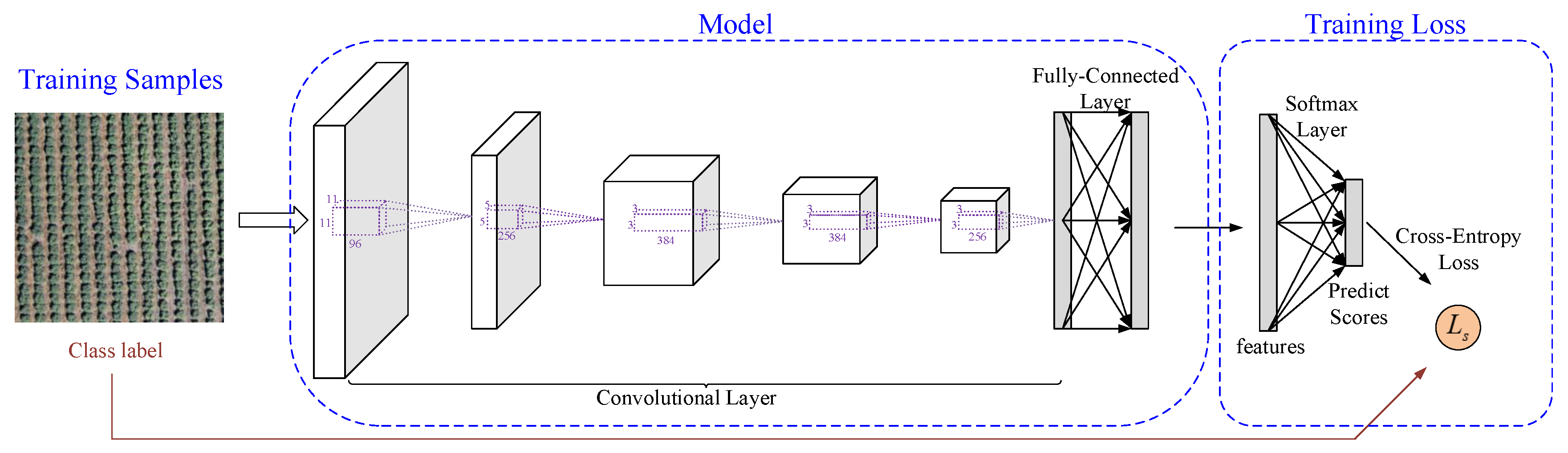
Generally, the CNNs can be seen as the parallel of layers where the features obtained by the former layer is performed as the input of the current layer. Figure 1 shows the architecture of the general CNNs that is used to obtain the representation of the remote sensing scenes. Let denote the features obtained in the layer, then the features obtained from the layer can be formulated as
where is the weights of the convolutional kernel and is the biases of the convolutional layer. is the non-linear activation function.
According to the requirements of different tasks, many CNN models, such as AlexNet [30], GoogLeNet [31], have been developed. Among these models, the AlexNet has obtained good performance in various computer vision tasks. It consists of five convolutional layers and two pooling layers. Each convolutional layer is followed by a ReLU layer as the activation function. Since this work mainly focuses on the training process of the deep model, this work will choose the AlexNet as the CNN model to generate feature representations from the remote sensing scenes.
Generally, the training batches which try to train the deep model simultaneously and accurately estimate the training model are used for the training process. The training batch denotes a batch of samples that are randomly selected from the whole training samples, which can train the model simultaneously and the average loss is used as the training loss. Denote B as the training batch and as the feature extracted from by the CNN. Given as the samples in the batch. Traditionally, the SoftMax loss which combines the SoftMax layer and the cross-entropy loss is used for the training of the CNNs. As Figure 1 shows, the SoftMax layer is used to transform the obtained features into the probability over each class. The cross-entropy loss, which is the penalization between the true and the predicted label, is usually used for the training of the CNNs. It can be formulated as
where denotes the weights of the SoftMax layer and is the bias term. denotes the number of elements in the set.
It can be noted from Equation (2) that the SoftMax loss tries to calculate the penalization point-to-point without considering the correlation between the training samples. This would limit the performance of the learned model especially for the remote sensing scenes with large intra-class variance and low inter-class variance, and the learned models are usually sub-optimal which cannot be fit for the requirement of the remote sensing scene tasks.
2.2. Structured Metric Learning
To further improve the representational ability of the learned deep model, the deep metric learning can be incorporated in the learning process to maximize the inter-class variance while minimizing the intra-class variance. This would be important especially for the remote sensing scenes since the scenes usually have similar characteristics between different classes.
To implement the deep metric learning, the key process is to calculate the difference between different samples. This work chooses the Mahalanobis distance as the metric to measure the distance between the obtained features from different samples. The distance can be calculated as
where represents the extracted feature from by the CNN. It should be noted that M is a symmetric semi-positive matrix and it can be decomposed as . Therefore, Equation (3) can be reformulated as
It can be noted from Equation (4) that H can be looked as a linear mapping on the learned features. Therefore, it acts like the fully connected layer of the deep model and can be implemented point-to-point in the training process of CNNs.
To make use of the pairwise correlation without constructing the positive and the negative pairs in the pre-training process, this work introduces the structured metric learning to maximize the inter-class variance and minimize the intra-class variance for the remote sensing scene classification [26]. Given , define as the set of samples with different labels from ,
where , represents the label of and , respectively. B is the training batch as former subsection shows. Then, the penalization from the negative pairs in the training batch (negative pair means pair of training samples with different class label) can be formulated as
where is a positive value. In the loss , the negative pairs of the sample , which is the nearest sample with different class labels from the sample in the batch B, and are penalized.
Define S as the set of positive pairs of the samples in training batch B (positive pair represents the pair of training samples with the same class label),
The penalization of the positive pairs in the batch B can be formulated as
Then, the loss for structured metric learning [26] penalizes the negative and positive pairs in each training batch, and it can be formulated as
The loss is used to train the CNN and encourage the learned features to be discriminative. The tries to maximize the difference between the learned features from samples in different classes and the tries to minimize the difference between the learned features from samples in the same class.
2.3. Center-Based Structured Metric Learning (C-SML) for Remote Sensing Scene Representation
Even though the structured metric learning optimizes the pairwise correlation between different training samples, the correlation between different classes has been ignored. To calculate the correlation between different classes, center points of different classes are introduced to represent each class. This work further measures the correlation between different classes via these center points.
To further decrease the intra-class variance, just as [27], we try to decrease the distances between the samples of each class and the corresponding center point. As Figure 2 shows, this just looks like a circle centered by the center point which tries to push all the samples of the class to the center point. Denote as the penalization term, and it can be formulated as [27]
where is the center point of class .
Moreover, all the center points are enforced to repulse from each other to further increase the inter-class variance. Since samples of each class is centered on the center point, encouraging different center point to repulse from each other just means the samples from different classes are enforced to be away from each other. Denote as the diversity-promoting term which encourages different center point repulse from each other. Then, the penalization can be formulated as
where is a positive value, represents the set of class labels and is the number of the labels.
Then, the penalization for the center points can be calculated as
This work tries to take advantage of the merits of both the structured metric learning and the center points. Therefore, the proposed center-based structured metric learning (C-SML) can be formulated as
where and are the tradeoff parameters, and calculate the penalization of the pairwise correlation and the classwise correlation of the training samples, respectively.
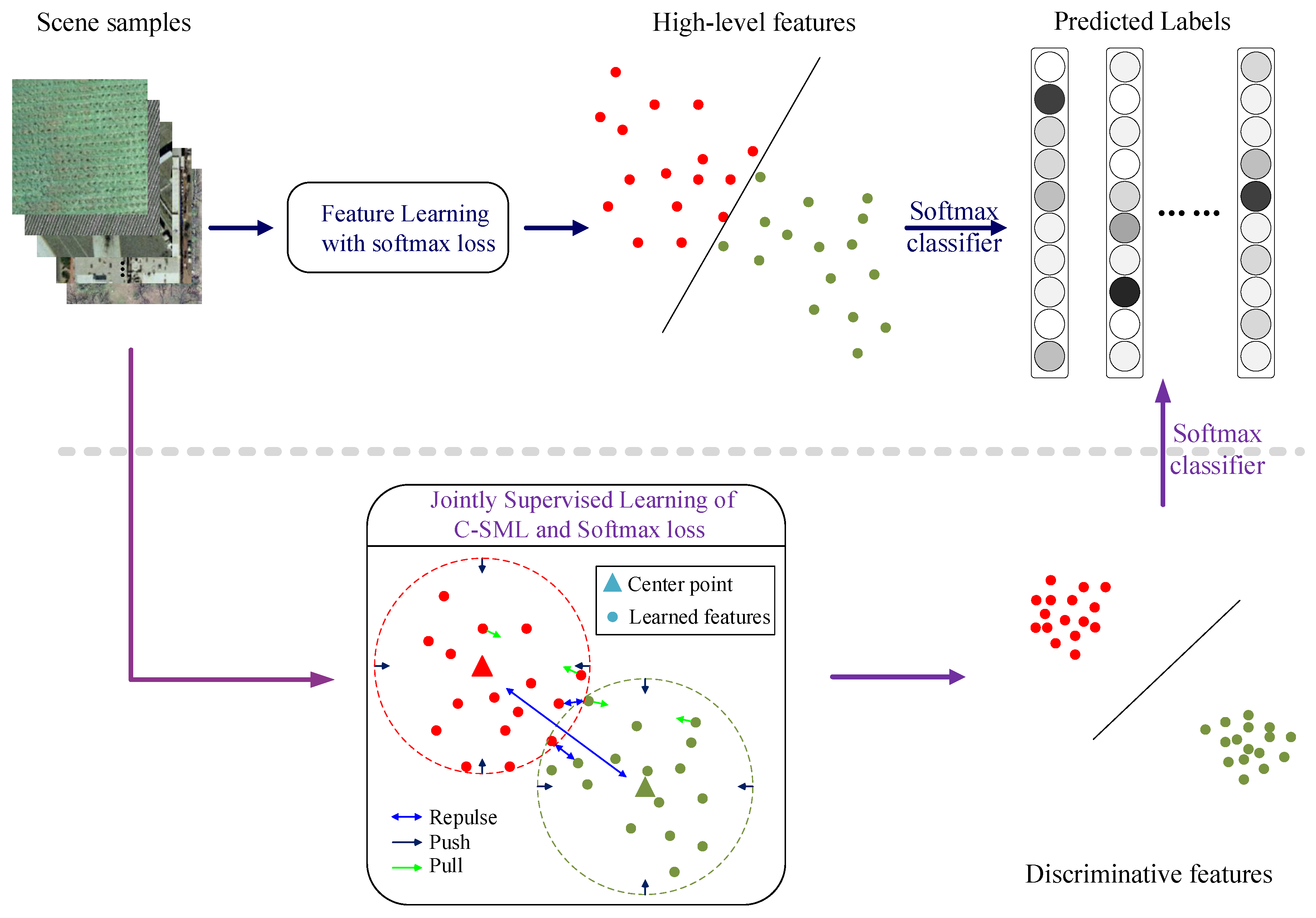
The effects of the proposed methods can be seen in Figure 2. From Figure 2, we can find that since the deep model can extract both the local and the global features from the samples, high-level features can be obtained from the samples and the performance can be significantly improved when compared with other “shallow” methods. Moreover, as Figure 2 shows, the proposed method pushes the samples of each class to the center point of the class and repulses different center point from each other. In addition, it pulls the samples of each class to each other and repulses different samples from each other to take advantage of the pairwise correlation. Therefore, the learned features would be more discriminative, and the classification performance would be further improved.
2.4. Implementation of the Proposed Method
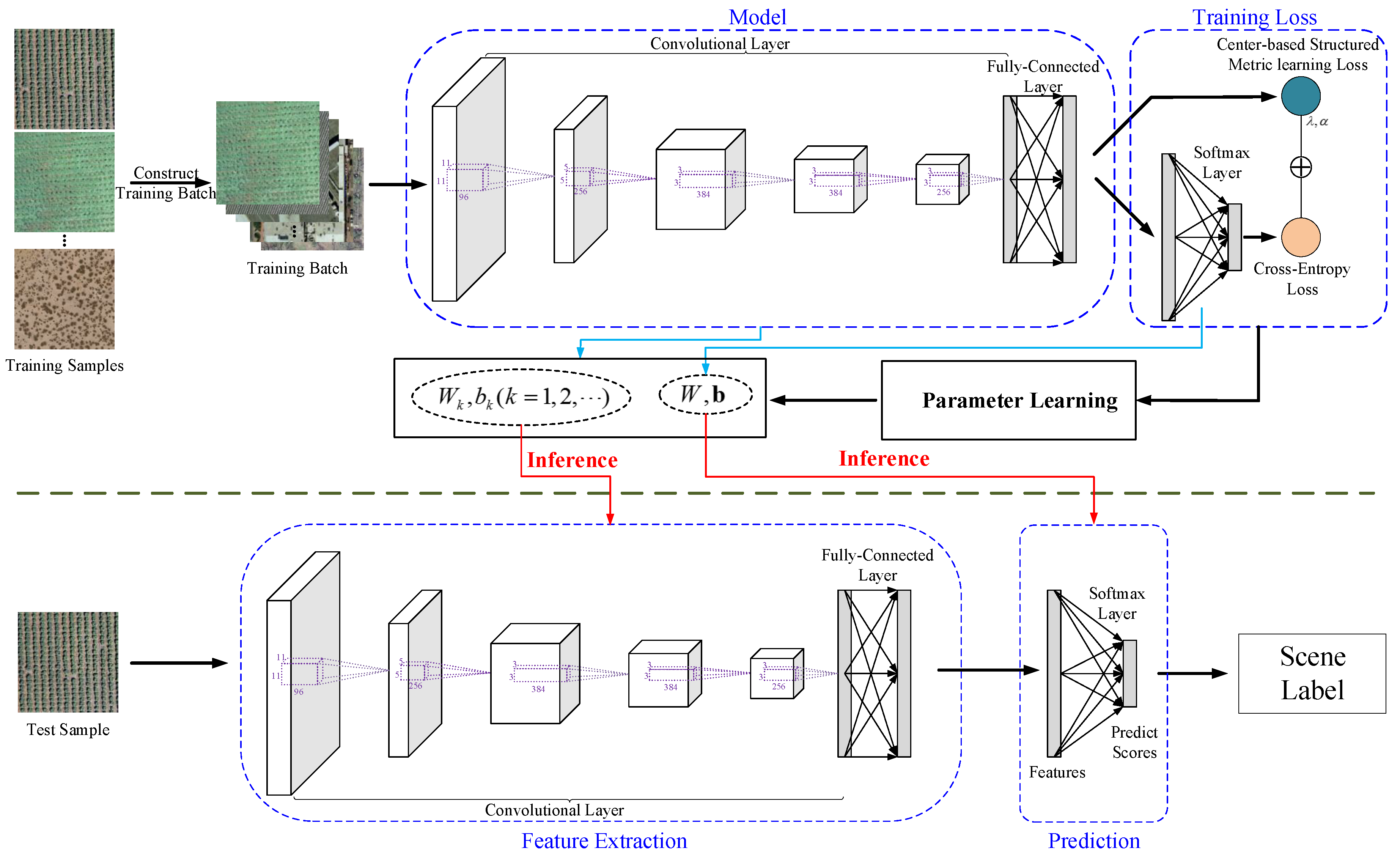
In this work, we want to train the SoftMax classifier and the CNNs simultaneously and use the point-wise information of each sample in the training process. Therefore, as Figure 3 shows, this work jointly learns the SoftMax loss and the center-based structured metric learning for the remote sensing scenes. The center-based structured metric learning loss tries to learn the parameters in the CNN model to encourage obtained features to be more discriminative. The SoftMax loss learns the CNN model with the parameters in the CNN model and the SoftMax layer. The joint loss can be formulated as
where calculates the cross-entropy loss which represents the point-wise penalization of each sample, calculates the penalization of pairwise correlation of training samples and measures the classwise correlation between different classes via the center points. and denote the positive values which act as the tradeoff parameters.
Generally, the CNNs supervised by the proposed method are trainable and can be optimized by the Stochastic Gradient Descent (SGD). Based on the characteristics of back propagation of deep models [32], the main problem is the partial of the proposed loss L w.r.t training samples in training batch B and the center point of each class. The partial of regarding can be implemented as Caffe and the partial of can be calculated as [26].
In addition, the partial of regarding can be calculated as
The partial of regarding can be calculated as
where represents the indicative function.
The partial of regarding can be calculated as
Therefore, the loss L w.r.t can be formulated as
The loss L w.r.t can be formulated as
The learning details of the proposed joint supervision are summarized in Algorithm 1. As Algorithm 1, in the training process, the parameters of the layer in the CNN model, which is used to extract features from the scenes, are updated with the center points (step 10 in Algorithm 1). Then, the center points are updated with the learned features from the CNN model (step 11 in Algorithm 1). Therefore, the center points and the deep metrics make the learned features from the CNN model be more discriminative, and the learned features from the CNN model encourage the center point to be close to the center of each class. As Figure 3 shows, the learned parameters of CNN model and the SoftMax layer are used to extract features from the scene and then the learned model is used to predict the class label of the scene.
| Algorithm 1 Implementation of the proposed method for remote sensing scene representation |
| Input: , as the parameter of the convolutional layer, W as the parameters and is the bias term in SoftMax layer, hyperparameter , learning rate , center points . |
| Output: , W, |
| 1: Initialize in convolution layer where is initialized from Gaussian distribution with standard deviation of 0.01 and is set to 0. |
| 2: Initialize the center points that each center point is filled with 0. |
| 3: while not converge do |
| 4: . |
| 5: Construct the training batch . |
| 6: Compute the supervised joint loss by . |
| 7: Compute the deviation regarding each in by . |
| 8: Compute the deviation w.r.t by . |
| 9: Update the parameters W by . |
| 10: Update the parameters of layer by . |
| 11: Update the center points by . |
| 12: end while |
| 13: return , W, |
3. Experimental Results
3.1. Experimental Datasets and Experimental Setup
To further validate the effectiveness of the proposed method, we conduct experiments on three real-world remote sensing image datasets with different properties. One of the datasets, which is called Brazilian Coffee Scene dataset [28], has multispectral high-resolution scenes. The other two, namely UC Merced Land-Use dataset [15], and Google dataset [5,33,34], are multi-class land-use datasets that contain high-resolution scenes in the visible spectrum.
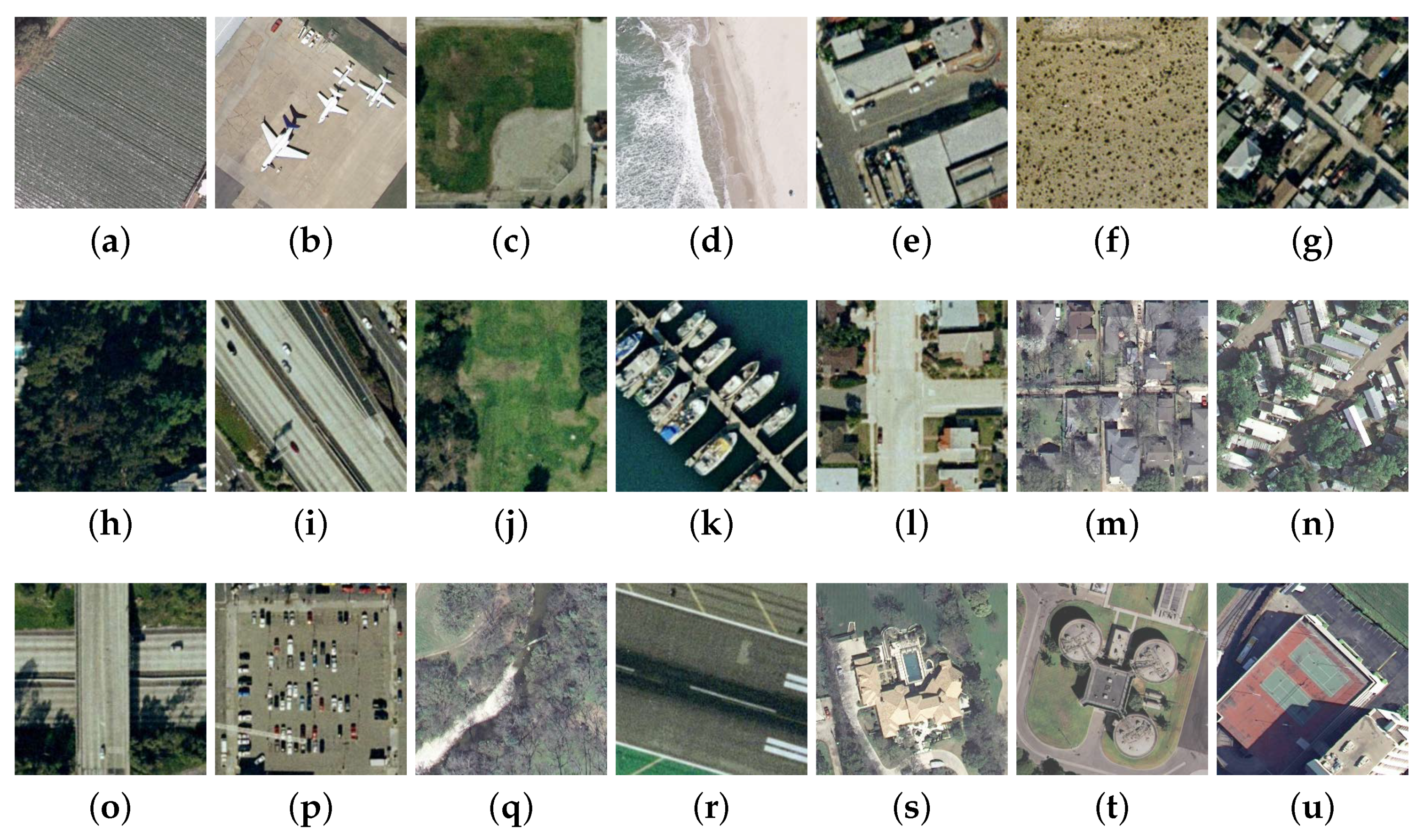
The UC Merced Land-Use Dataset was manually extracted from aerial orthoimagery with a resolution of one foot per pixel. The dataset has 2100 aerial scene images with pixels divided into 21 challenging scene classes (see Figure 4 for details). It contains some highly overlapping categories, such as the sparse residential and the dense residential, the forest and the mobile home park, which make it difficult to discriminate different scenes.
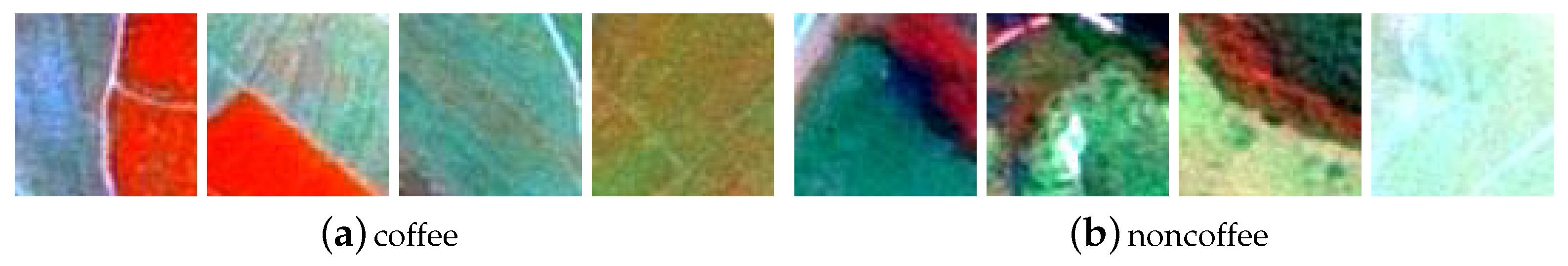
The Brazilian coffee scenes were taken by the SPOT sensor in the green, red, and near-infrared bands. The dataset contains 2876 scenes with pixels which can be divided into 2 classes, namely coffee and noncoffee(see Figure 5 for details). The differences in the resolution, and spectral in the scenes make it more complicated than those in the UC Merced and Google data sets.
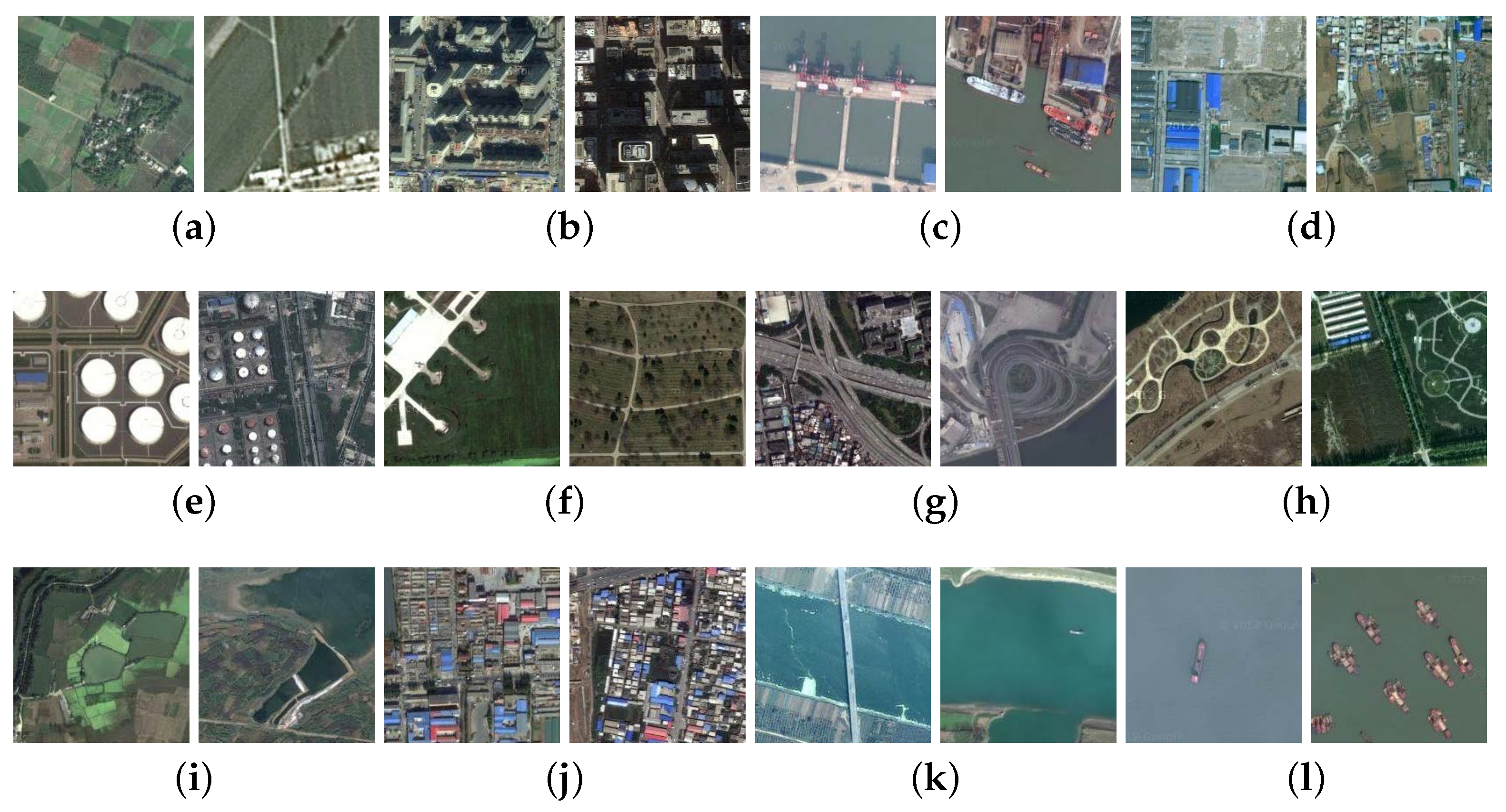
The Google Dataset was collected from Google Earth by SIRI-WHU and mainly covers the urban areas in China. Each scene image has with a 2-m spatial resolution. The dataset contains 2400 scenes which are divided into 12 classes, including agriculture, commercial, harbor, idle land, industrial meadow, overpass, park, pond residential, river, and water (see Figure 6 for details). Compared with UC Merced, the dataset represents the performance of the method over dataset with relatively low resolution.
In the experiments, all the datasets have been equally divided into five folds where four of the folds are used for training and the remainder is used for testing. Therefore, all the experimental results are obtained by the five-fold cross-validation. For UC Merced Land-Use dataset and Google dataset, 70%, 10%, 20% of labeled samples are used for training, validation, and testing, respectively. For Brazilian Coffee dataset, 90% of the training samples are used for training and the remainder for validation.
All the deep models are implemented on Caffe [35] which is a popular deep learning framework. SoftMax classifier is chosen as the classifier to classify different scenes. In addition, as Section 2.1 introduces, AlexNet is chosen as the deep model to learn the features from the scenes for all the three datasets. Since the three datasets used in this work have different dimensions, we use the crop technology and change the parameter in the first convolutional layer for different datasets. For UC Merced Land-Use dataset, the setup is similar to original AlexNet. For Brazilian Coffee Scene dataset, the crop size of the scenes is set to 63, and the kernel size and the stride in the first convolutional layer are set to 9 and 1, separately. While for Google dataset, the crop size of the scenes is set to 173, and the kernel size and the stride in the first convolutional layer are set to 11 and 3, respectively. Through the adjustment, the outputs from the first convolutional layer of the three datasets are the same and we can use the pre-trained model from ImageNet for transferring learning. Very common machine with a 3.4 GHz Intel (R) Core i7 and a GeForce GT 1080 8 GB GPU is chosen to test the performance of the proposed method.
3.2. Classification Performance with Different and
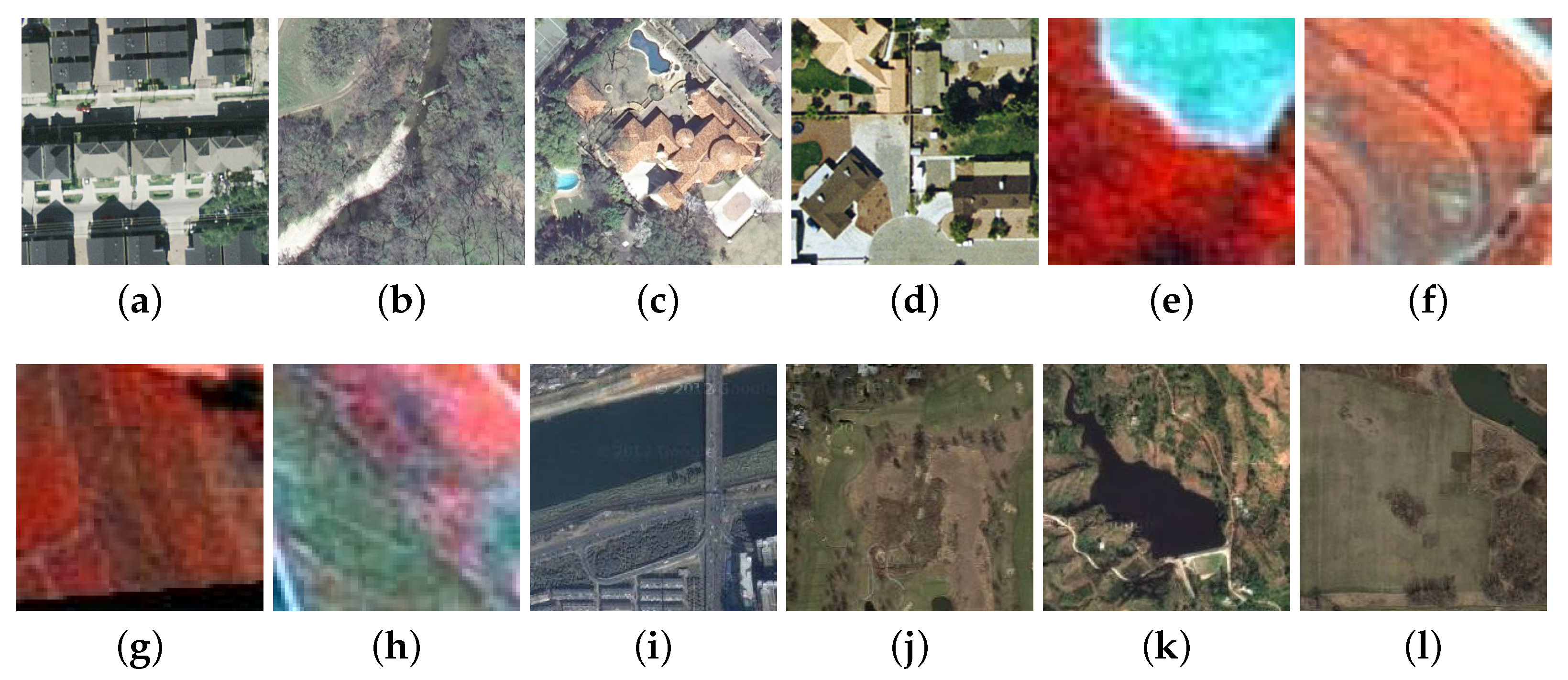
The proposed joint learning of C-SML and SoftMax loss take advantage of the point-wise, pairwise and the classwise information to increase the inter-class variance and decrease the intra-class variance, and thus it can significantly improve the representational ability for the remote sensing scenes. The classification results of the methods are listed in Table 1. It should be noted that the center-SoftMax means the joint learning of the center points and the SoftMax loss. The SML-SoftMax means the joint learning of the structured metric learning and the SoftMax loss. Figure 7 presents examples of samples which are wrongly classified by other methods but correctly classified by the proposed method. We can find that even the overlapping samples, such as the medium residential and dense residential in Figure 7d, and the meadow and the agriculture in Figure 7l can be discriminated by the proposed method. Therefore, from the table and the figure, it can be noted that the proposed method can significantly improve the representational ability for the remote sensing scenes.
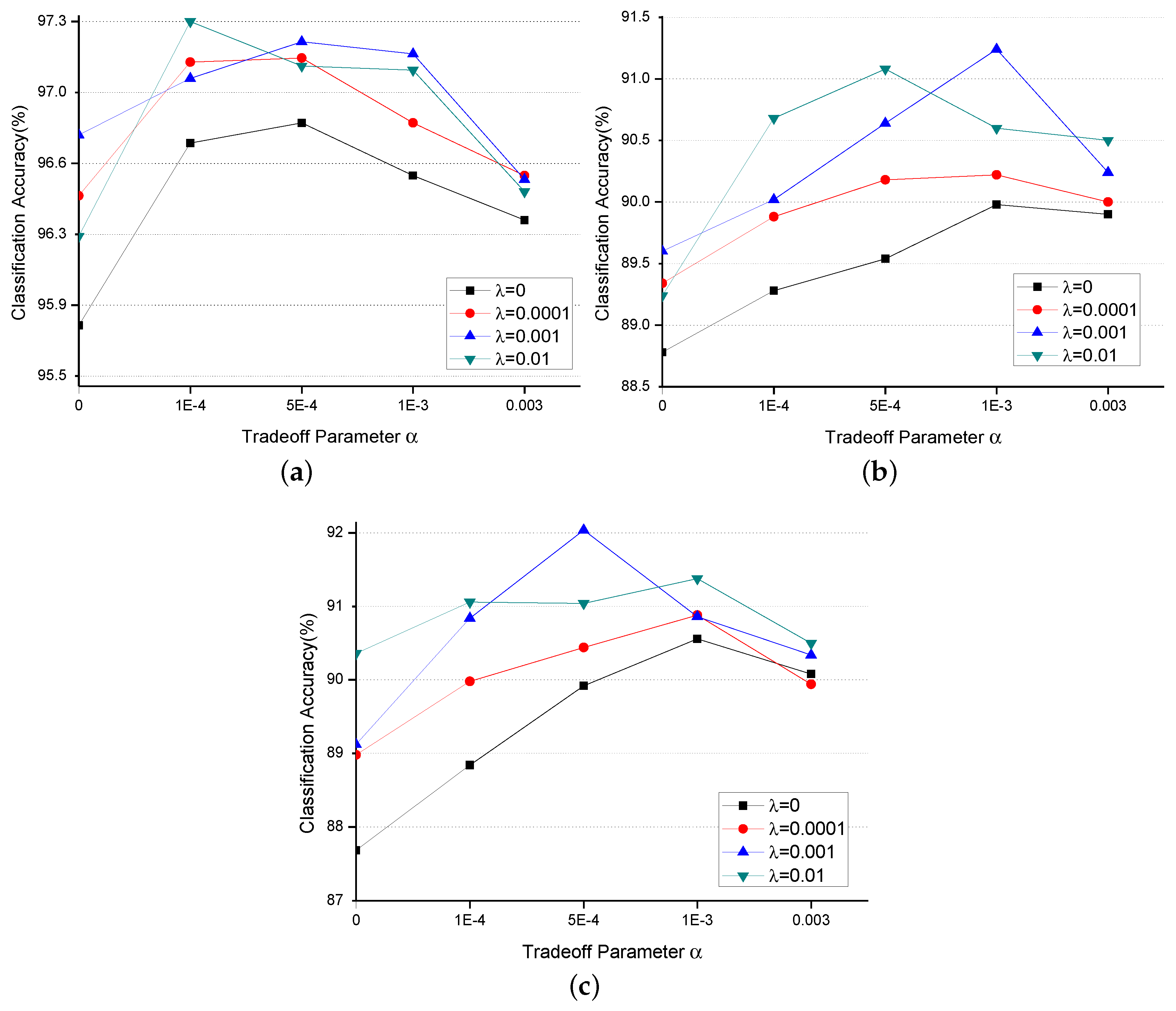
However, it should be noted that the performance of the proposed joint learning method is affected by the hyperparameter and . The classification results over the three datasets with different and is shown in Figure 8. In the experiments, the parameter is set to 0, 0.0001, 0.001, 0.01 and the is set to 0, 0.0001, 0.0005, 0.001, 0.003, respectively. We can find from Figure 8a,b that the proposed method achieves when and and when and on UC Merced Land-Use dataset and Brazilian Coffee Scene coffee dataset which ranks the best, respectively. In addition, from Figure 8c, it can be noted that the proposed method ranks the best when and for the Google dataset.
When we fixed the hyperparameter , the results in Figure 8 would show the effects of the classwise correlation between different classes on the classification performance for remote sensing scenes. From the trend of performance with different hyperparameter, we can find that the classification performance over the three datasets increases with the increase of the hyperparameter . In particular, the classification performance is significantly improved when compared with that when . This means the classwise correlation from the center points has positive effects in the performance of remote sensing scene representation. However, we should also note that when is extensively large, the performance decreases. In particular, when the value of is larger than 0.003, the learned model would not converge. That is because that when is too large, the learning process pays too much attention on the learning of center points while ignores the optimization of the model. In addition, it should be noted that when , the classification results show the performance of joint learning of center points and the SoftMax loss. For UC Merced Land-Use dataset, the performance ranks the best () when . The classification results can rank and when over the Brazilian Coffee Scene dataset and the Google dataset.
When we fixed the hyperparameter , the results in Figure 8 show the effects of the pairwise correlation between different samples on the classification performance for remote sensing scenes. Inspect the classification accuracy in Figure 8 and it can obtain the following conclusions.
- The joint learning of pairwise correlation and the point-wise information shows positive effects on the representational ability of the learned model for remote sensing scenes. It can be noted that in Figure 8a,b the lines of classification accuracies when is above the line when . Moreover, in Figure 8c, the classification performance is better with pairwise correlation except when . The use of pairwise correlation for the training process increases the inter-class variance and decreases the intra-class variance of the remote sensing scenes and thus encourages the learned model to better represent the scenes.
- The larger of the hyperparameter value is, the higher the classification accuracy is. Larger value means the more pairwise correlation is used in the training process. This would avoid some bad local optimum in the training process and thus increase the representational ability of the learned model.
It is worthwhile to note that in the experiments, we choose five-fold cross-validation to obtain the results. The classification performance over different folds has great changes. For example, over Google dataset, the average accuracies over center-SoftMax and proposed method are and , respectively. The classification accuracies over the five folds by the center-SoftMax are 89.4%, 90.3%, 91.5%, 91.7%, 89.9% while the accuracies by the proposed method can be 90.7%, 92.9%, 93.1%, 92.5%, 91%, respectively. We can find that the proposed method obtains a better performance over all the five folds.
In conclusion, both the and have significant effects on the classification performance of remote sensing scenes. It is important to choose a proper one in the experiments. In real-world application, cross-validation could be used to choose a proper value for the hyperparameter with different computer vision tasks.
3.3. Comparisons of Different Methods
To comprehensively evaluate the proposed method, three classes of baselines have been chosen for the comparisons over the three datasets. First, the joint learning method of the center points and the SoftMax loss is compared with the traditional deep models learned with SoftMax loss to show the performance of the using of classwise correlation for the remote sensing scenes. Second, we compare the results of the joint learning method of the structured metrics and the SoftMax loss with those of the traditional deep models learned with SoftMax loss to show the effects of pairwise correlation between the training samples in the performance of remote sensing scene classification. Then, the results of the joint learning of the proposed C-SML and the SoftMax loss is compared with those obtained with pairwise and point-wise correlation. Finally, we compare the results of the proposed joint learning method with those obtained with classwise and point-wise correlation. To further compare the classification performance, we list the confusion matrix of different methods in Figure 9, Figure 10 and Figure 11.
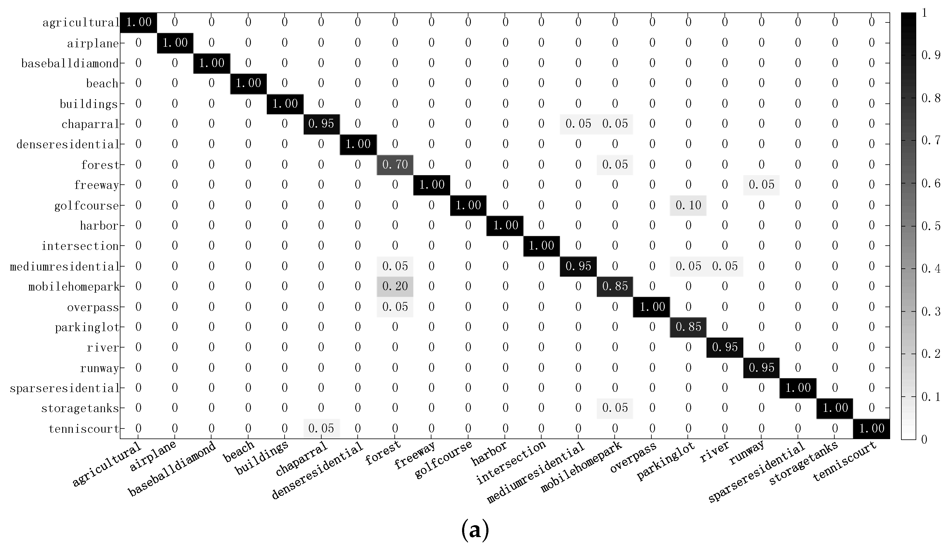
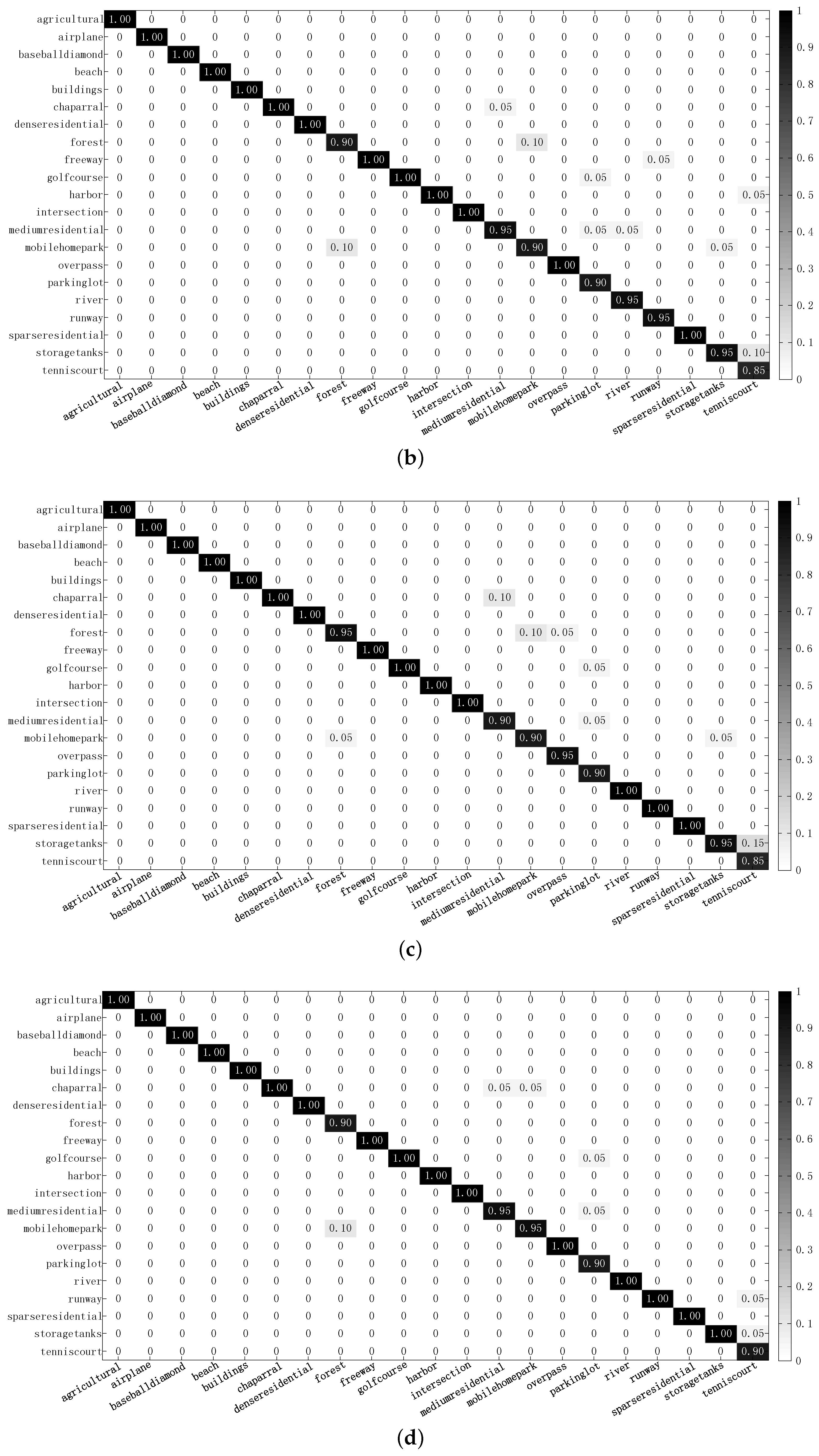
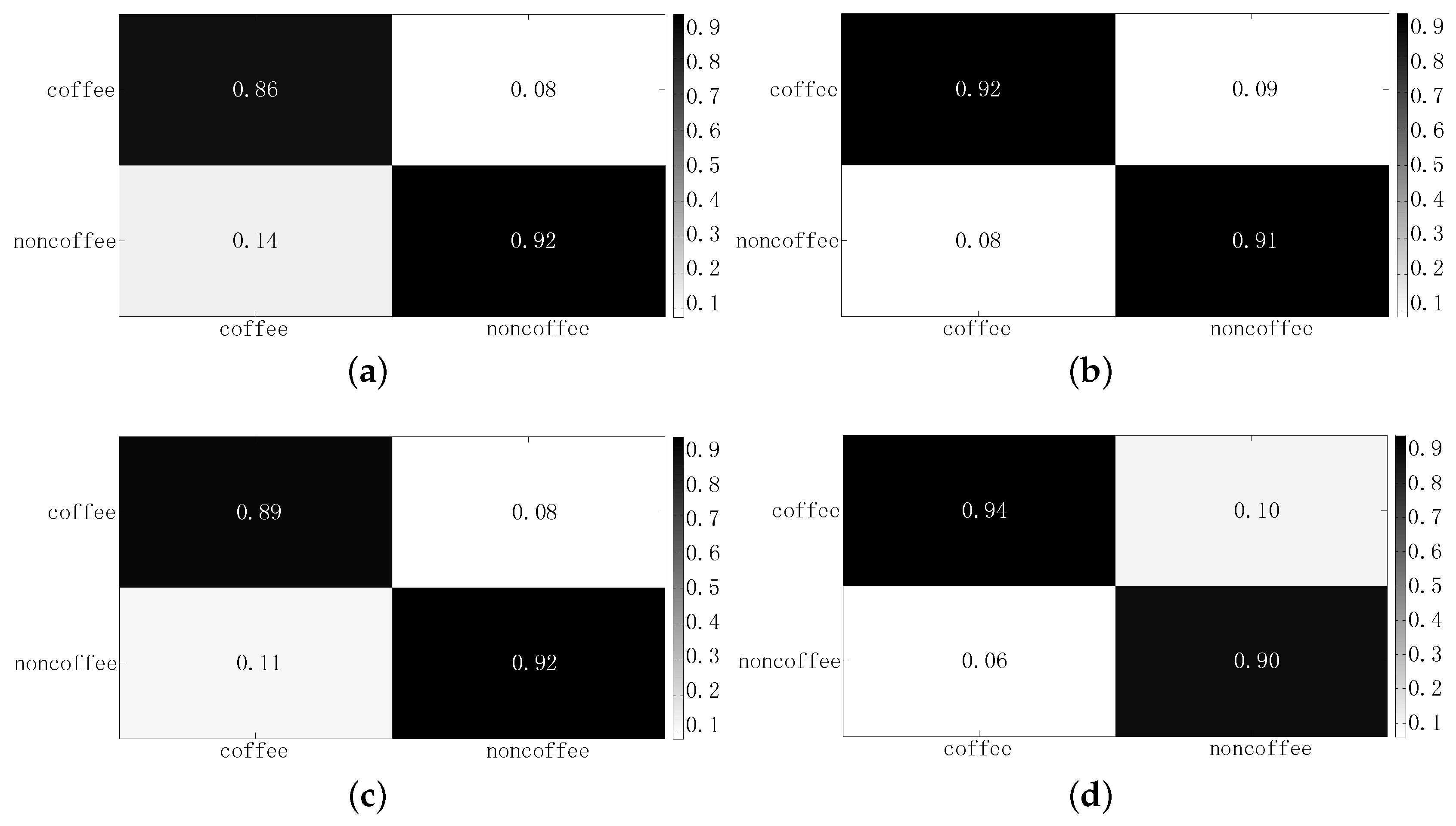
First, the results from the joint learning of the center points and the SoftMax loss are compared with that obtained from the learning with SoftMax loss. As introduction shows, Since the remote sensing scenes usually have complex arrangements and limited training samples, the learned model usually tends to be local optimal which limits the representational ability for the scenes [9,36]. Through incorporating the classwise into the training process, the learned model could better represent the scenes. Compare the a and b in Figure 9, Figure 10 and Figure 11, and we can find that the structured metric learning can make the model converge to the global optimum or a better local optimum, which could improve the representational ability for remote sensing scenes. For example, Over UC Merced Land-Use dataset, the classification errors of forest/mobilehomepark, and parkinglot/golfcourse decrease by 50% and the classification errors of forest/overpass, chaparral/tenniscourt, mobilehomepark/storagetanks, forest/mediumresidential, and mobilehomepark/chaparral decrease by 100%. For Brazilian Coffee Scene dataset, the classification error of coffee/noncoffee decreases by 42.9%. For Google dataset, the classification errors of some classes with low inter-class variance, such as idle land/agriculture, commercial/park, harbor/park, overpass/park, industrial/overpass, river/pond, harbor/pond, idle land/meadow, decrease by 100%. These improvements make the significant improvement of the whole classification performance. From Table 1, we can find that the average accuracy of the joint learning method ranks 96.80%, 89.98% and 90.56% which are higher than 95.80%, 88.78% and 87.68% over UC Merced Land-Use, Brazilian Coffee Scene dataset, and Google dataset, respectively.
Then, Table 1 also demonstrates that the joint learning of the structured metric learning and the SoftMax loss obtains better results than the traditional CaffeNet trained with SoftMax loss. From Table 1, we can find that the average accuracy of the joint learning method ranks 96.74%, 89.60% and 90.36% which are higher than 95.80%, 88.78% and 87.68% over UC Merced Land-Use, Brazilian Coffee Scene dataset, and Google dataset, respectively. Different from the center points, the structured metrics encourage the learned model to a better one through increasing the pairwise distances from different classes and minimizing the pairwise distances within each class. Compare a and c in Figure 9 and Figure 10, we can also find the joint learning method provides better representation for the remote sensing scenes.
Finally, compare the joint learning of SML-SoftMax with the proposed method, we can find that the proposed method obtains significant improvement on both the datasets. Moreover, compare the joint learning of center-SoftMax with the proposed method, we can also find that the proposed method obtains significant improvement on both the datasets. From Figure 9b–d, Figure 10b–d and Figure 11b–d, we can find that the proposed method, which makes use of the classwise, pairwise and the point-wise correlation of the training samples in the training process, can improve the representational ability of the learned model with the SML-SoftMax and the center-SoftMax. For UC Merced Land-Use dataset, we can find the classification errors of some overlapping classes, such as storagetanks/mobilehomepark, mobilehomepark/forest, decrease by 100% with the proposed method when compared with other two. In addition, the classification error of tenniscourt/storagetanks decreases by 50% and 66.7% when compared with the Center-SoftMax and the SML-SoftMax, respectively. For Brazilian Coffee Scene dataset, the classification error of coffee/noncoffee decreases by 25% and 45.5% with the Center-SoftMax and the SML-SoftMax separately. In addition, for Google dataset, the classification errors of some similar classes, such as the river/harbor, overpass/commercial, harbor/overpass, pond/park, residential/overpass, decrease by 100%. The classification errors of meadow/agriculture, water/harbor, and commercial/residential decrease by 70%, 40%, 40%, respectively. Some other classification errors, such as the overpass/idle and, harbor/river, pond/river, have also significantly decreased by the proposed method. Overall, the proposed method which take advantage of the classwise, pairwise, and the point-wise correlation, can significantly improve the classification performance for remote sensing scenes.
To be concluded, by introducing a center point in the metric learning, the inter-class variance is increased, and the intra-class variance is decreased. The features obtained from the proposed method can be more discriminative and easily separated.
3.4. Comparisons with the Most Recent Methods
To further validate the effectiveness of the proposed method, the performance of the proposed method is compared with the performance of the state-of-the-art methods. The comparisons of the UC Merced Land-Use dataset, the Brazilian Coffee Scene dataset, and the Google dataset can be seen in Table 2, Table 3 and Table 4, respectively. In these tables, we use the experimental results of other recent methods from the paper with the same experimental setups directly.
The table lists the SIFT [9] and DMTM [5] as the baseline of the “shallow” methods. From the comparisons, we can find that when compared with the “shallow” methods, the proposed method outperforms these methods on both the datasets. Over UC Merced Land-Use dataset, the proposed method obtains 97.30% which is higher than 78.81%, 72.05%, 91.38%, 91.63% and 92.92% which are obtained by SIFT [9], BOVW [34], FK-O [34], FK-S [34] and DMTM [5], respectively. Over Brazilian Coffee Scene dataset, the proposed method obtains 91.24% which is better than that obtained by SIFT [9] (82.83%). For Google dataset, the proposed method can obtain 92.04% which outperforms the SIFT [5], DMTM [5], BOVW [34], FK-O [34], FK-S [34], respectively. Since the SIFT, DMTM, BOVW, FK-O and FK-S are typical “shallow” methods, the comparisons demonstrate that the proposed method which is the deep representation is better than these “shallow” methods.
From Table 2, Table 3 and Table 4, we can also find that when compared with other deep methods, the proposed method can also obtain comparable or even better performance. For UC Merced Land-Use dataset, the proposed method can obtain 97.30% which is better than that obtained by CaffeNet (95.48%) [7] and D-DSML-CaffeNet (96.76%) [9] which is based on CaffeNet. It can be also noted that the proposed method outperforms other deep models, such as GoogLeNet [7] which obtains 97.10%, VGG-VD16-1st-FC+Aug [23] which obtains 96.88%, SPP-net+MKL [29] which obtains 96.38%, and MCNN [21] which obtains 96.66%. For Brazilian Coffee Scene dataset, the proposed method also obtains 91.24% outperforms 88.46% which is obtained by LQPCANet [37], 85.36% by VGG16 [22], 89.79% by ConvNet [38], 90.94% by CaffeNet [7] and 91.13% by D-DSML-CaffeNet [9]. For Google dataset, the proposed method obtains 92.04% which is better than 82.81% by TF-CNN [39], 89.88% by RDSG-CNN [39], 87.68% by Fine-tuned CaffeNet. Therefore, when compared with other deep methods, the proposed method shows better performance.
The experimental results over three real-world remote sensing scene datasets demonstrate that the proposed method which considers the merits of the point-wise, pairwise and the classwise information, can improve the representational ability for the remote sensing scenes and obtain better classification performance when compared with the most recent methods.
4. Conclusions and Discussions
In this paper, a novel jointly supervised learning of the C-SML and the SoftMax loss is developed for remote sensing scene classification to learn the CNN model and the classifier simultaneously. First, the center points, which are used to represent the center of the learned features, have been introduced to the training process deep model for remote sensing scene representation. Experimental results have shown that the center points can improve the representational ability of the model and the learned features can be more discriminative. Then, this work develops the center-based structured metric learning which take both the pairwise and the classwise of the training samples into consideration. Through decreasing the intra-class variance and maximizing the inter-class variance with the proposed C-SML, the representational ability of the model for remote sensing scenes can be further improved. Experimental results have shown that the deep model learned with the C-SML can better fit for the remote sensing scenes. In particular, some scenes with great similarity can be discriminated. Finally, the joint learning of the C-SML and the SoftMax loss is developed to train the model point-to-point. The developed joint learning method is easy to implement. Moreover, the joint learning can take advantage of the point-wise information from the SoftMax loss, and the pairwise and classwise information from the C-SML, which can further improve classification performance for remote sensing scenes. The experimental results have shown that the proposed method can obtain comparable or even better results than other state-of-the-art methods over the three datasets.
This work only demonstrates the powerful ability of the joint learning of the center points and deep metrics over the UC Merced Land-Use, Brazilian Coffee Scene and Google dataset. In future work, we intend to apply the proposed method in other types of images such as hyperspectral image. Since remote sensing scenes usually cannot provided enough training samples, the use of the center points to formulate pseudo classes for unsupervised deep learning for remote sensing scene representation is another interesting future work. In addition, we would like to evaluate the performance of the proposed method on other CNN models, such as GoogLeNet and ResNet.
Author Contributions
All the authors made significant contributions to the work. Z.G. and P.Z. developed the methods, conducted experiments and finally analyzed the results. W.H. and Y.H. provided advices for the preparation and revision of the paper.
Funding
This research was funded in part by the Natural Science Foundation of China under Grant 61671456 and 61271439, in part by the Foundation for the Author of National Excellent Doctoral Dissertation of China (FANEDD) under Grant 201243, and in part by the Program for New Century Excellent Talents in University under Grant NECT-13-0164.
Acknowledgments
In this section you can acknowledge any support given which is not covered by the author contribution or funding sections. This may include administrative and technical support, or donations in kind (e.g., materials used for experiments).
Conflicts of Interest
The authors declare no conflict of interest.
References
- Cheriyadat, A.M. Unsupervised feature learning for aerial scene classification. IEEE Trans. Geosci. Remote Sens. 2014, 52, 439–451. [Google Scholar] [CrossRef]
- Zhang, F.; Du, B.; Zhang, L. Saliency-guided unsupervised feature learning for scene classification. IEEE Trans. Geosci. Remote Sens. 2015, 53, 2175–2184. [Google Scholar] [CrossRef]
- Ren, S.; He, K.; Sun, J. Faster R-CNN: Towards real-time object detection with region proposal networks. IEEE Trans. Pat. Anal. Mach. Intell. 2017, 6, 1137–1149. [Google Scholar] [CrossRef] [PubMed]
- Lin, T.Y.; Dollar, P.; Girshick, R.B.; He, K.; Hariharan, B.; Belongie, S.J. Feature Pyramid Networks for Object Detection. In Proceedings of the IEEE Conference on Computer Vision and Pattern Recognition, Honolulu, HI, USA, 21–26 July 2017; pp. 2117–2125. [Google Scholar]
- Zhao, B.; Zhong, Y.; Xia, G.; Zhang, L. Dirichlet-Derived Multiple Topic Scene Classification Model for High Spatial Resolution Remote Sensing Imagery. IEEE Trans. Geosci. Remote Sens. 2016, 54, 2108–2123. [Google Scholar] [CrossRef]
- Huang, B.; Zhao, B.; Song, Y. Urban land-use mapping using a deep convolutional neural network with high spatial resolution multispectral remote sensing imagery. Remote Sens. Environ. 2018, 214, 73–86. [Google Scholar] [CrossRef]
- Castelluccio, M.; Poggi, G.; Sansone, C.; Verdoliva, L. Land use classification in remote sensing images by convolutional neural networks. arXiv, 2015; arXiv:1508.00092. [Google Scholar]
- Taylor, J.R.; Lovell, S.T. Mapping public and private spaces of urban agriculture in chicago through the analysis of high-resolution aerial images in google earth. Landsc. Urban Plan. 2012, 108, 57–70. [Google Scholar] [CrossRef]
- Gong, Z.Q.; Zhong, P.; Yu, Y.; Hu, W.D. Diversity-Promoting Deep Structural Metric Learning for Remote Sensing Scene Classification. IEEE Trans. Geosci. Remote Sens. 2018, 56, 371–390. [Google Scholar] [CrossRef]
- Zhong, Y.; Zhu, Q.; Zhang, L. Scene Classification Based on the Multifeature Fusion Probabilistic Topic Model for High Spatial Resolution Remote Sensing Imagery. IEEE Trans. Geosci. Remote Sens. 2015, 53, 6207–6222. [Google Scholar] [CrossRef]
- Kahaki, S.M.M.; Nordin, M.J.; Ashtari, A.H. Contour-based corner detection and classification by using mean projection transform. Sensors 2014, 14, 4126–4143. [Google Scholar] [CrossRef]
- Chen, S.; Tian, Y. Pyramid of spatial relatons for scene-level land use classification. IEEE Trans. Geosci. Remote Sens. 2015, 53, 1947–1957. [Google Scholar] [CrossRef]
- Charalampidis, D.; Kasparis, T. Wavelet-based rotational invariant roughness features for texture classification and segmentation. IEEE Trans. Image Process. 2002, 11, 825–837. [Google Scholar] [CrossRef] [PubMed] [Green Version]
- Chen, C.; Zhang, B.; Su, H.; Li, W.; Wang, L. Land use scene classification using multi-scale completed local binary patterns. Signal Image Video Process. 2016, 10, 745–752. [Google Scholar] [CrossRef]
- Yang, Y.; Newsam, S. Bag-of-visual-words and spatial extensions for land-use classification. In Proceedings of the 18th SIGSPATIAL International Conference on Advances in Geographic Information Systems, San Jose, CA, USA, 2–5 November 2010; pp. 270–279. [Google Scholar]
- Ren, J.; Jiang, X.; Yuan, J. Learning LBP structure by maximizing the conditional mutual information. Pattern Recognit. 2015, 48, 3180–3190. [Google Scholar] [CrossRef]
- Kahaki, S.M.M.; Nordin, M.J.; Ashtari, A.H.; Zahra, S.J. Invariant feature matching for image registration application based on new dissimilarity of spatial features. PLoS ONE 2016, 11, e0149710. [Google Scholar]
- Zhong, P.; Gong, Z.Q.; Li, S.; Schönlieb, C.B. Learning to diversify deep belief networks for hyperspectral image classification. IEEE Trans. Geosci. Remote Sens. 2017, 55, 3516–3530. [Google Scholar] [CrossRef]
- Liu, W.; Wen, Y.; Yu, Z.; Li, M.; Raj, B.; Song, L. Sphereface: Deep hypersphere embedding for face recognition. In Proceedings of the IEEE Conference on Computer Vision and Pattern Recognit, Honolulu, HI, USA, 21–26 July 2017; pp. 212–220. [Google Scholar]
- Liu, W.; Anguelov, D.; Erhan, D.; Szegedy, C.; Reed, S.; Fu, C.Y.; Berg, A.C. SSD: Single shot multibox detector. In Proceedings of the European Conference on Computer Vision, Amsterdam, The Netherlands, 8–16 October 2016; pp. 21–37. [Google Scholar]
- Liu, Y.; Zhong, Y.; Qin, Q. Scene Classification Based on Multiscale Convolutional Neural Network. IEEE Trans. Geosci. Remote Sens. 2018, 56, 7109–7121. [Google Scholar] [CrossRef]
- Nogueira, K.; Penatti, O.A.; dos Santos, J.A. Towards better exploiting convolutional neural networks for remote sensing scene classification. Pattern Recognit. 2017, 61, 539–556. [Google Scholar] [CrossRef] [Green Version]
- Hu, F.; Xia, G.S.; Hu, J.; Zhang, L. Transferring deep convolutional neural networks for the scene classification of high-resolution remote sensing imagery. Remote Sens. 2015, 7, 14680–14707. [Google Scholar] [CrossRef]
- Wang, J.; Zhou, F.; Wen, S.; Liu, X.; Lin, Y. Deep Metric Learning with Angular Loss. In Proceedings of the 2017 IEEE International Conference on Computer Vision (ICCV), Venice, Italy, 22–29 October 2017; pp. 2612–2620. [Google Scholar]
- Sohn, K. Improved deep metric learning with multi-class N-pair loss objective. In Proceedings of the Advances in Neural Informaiton Processing Systems, Barcelona, Spain, 5–10 December 2016; pp. 1857–1865. [Google Scholar]
- Oh Song, H.; Xiang, Y.; Jegelka, S.; Savarese, S. Deep metric learning via lifted structured feature embedding. In Proceedings of the IEEE Conference on Computer Vision and Pattern Recognition, Las Vegas, NV, USA, 27–30 June 2016; pp. 4004–4012. [Google Scholar]
- Wen, Y.; Zhang, K.; Li, Z.; Qiao, Y. A discriminative feature learning approach for deep face recognition. In Proceedings of theEuropean Conference on Computer Vision, Amsterdam, The Netherlands, 8–16 October 2016; pp. 499–515. [Google Scholar]
- Penatti, O.A.B.; Nogueira, K.; dos Santos, J.A. Do deep features generalize from everyday objects to remote sensing and aerial scenes domains? In Proceedings of the IEEE Conference on Computer Vision and Pattern Recognition Workshops, Boston, MA, USA, 7–12 June 2015; pp. 44–51. [Google Scholar]
- Liu, Q.; Hang, R.; Song, H.; Li, Z. Learning multi-scale deep features for high-resolution satellite image classification. IEEE Trans. Geosci. Remote Sens. 2018, 56, 117–126. [Google Scholar] [CrossRef]
- Krizhevsky, A.; Sutskever, I.; Hinton, G.E. Imagenet classification with deep convolutional neural networks. In Proceedings of the Advances in Neural Information Processing Systems, Lake Tahoe, NV, USA, 3–6 December 2012; pp. 1097–1105. [Google Scholar]
- Szegedy, C.; Liu, W.; Jia, Y.; Sermanet, P.; Reed, S.; Anguelov, D.; Erhan, D.; Vanhoucke, V.; Rabinovich, A. Going deeper with convolutions. In Proceedings of the IEEE Conference on Computer Vision and Pattern Recognition, Boston, MA, USA, 7–12 June 2015; pp. 1–9. [Google Scholar]
- Haykin, S.S. Nerual Networks and Learning Machines; Pearson: Upper Saddle River, NJ, USA, 2009. [Google Scholar]
- Zhu, Q.; Zhong, Y.; Zhao, B.; Xia, G.S.; Zhang, L. Bag-of-visual-words scene classifier with local and global features for high spatial resolution remote sensing imagery. IEEE Geosci. Remote Sens. Lett. 2016, 13, 747–751. [Google Scholar] [CrossRef]
- Zhao, B.; Zhong, Y.; Zhang, L.; Huang, B. The Fisher Kernel Coding Framework for High Spatial Resolution Scene Classification. Remote Sens. 2016, 8, 157. [Google Scholar] [CrossRef]
- Jia, Y.; Shelhamer, E.; Donahue, J.; Karayev, S.; Long, J.; Girshick, R.; Guadarrama, S.; Darrell, T. Caffe: Convolutional architecture for fast feature embedding. In Proceedings of the ACM International Conference on Multimedia, Orlando, FL, USA, 3–7 November 2014; pp. 675–678. [Google Scholar]
- Gong, Z.Q.; Zhong, P.; Hu, W.D. Diversity in Machine Learning. arXiv, 2018; arXiv:1807.01477. [Google Scholar]
- Wang, J.; Luo, C.; Huang, H.; Zhao, H.; Wang, S. Transferring pre-trained deep CNNs for remote scene classification with general features learned from linear PCA Network. Remote Sens. 2017, 9, 225. [Google Scholar] [CrossRef]
- Nogueira, K.; Miranda, W.O.; Dos Santos, J.A. Improving spatial feature representation from aerial scenes by using convolutional networks. In Proceedings of the 2015 28th SIBGRAPI Conference on Graphics, Patterns and Images (SIBGRAPI), Salvador, Bahia, Brazil, 26–29 August 2015; pp. 289–296. [Google Scholar]
- Zhong, Y.; Fei, F.; Zhang, L. Large patch convolutional neural networks for the scene classification of high spatial resolution imagery. J. Appl. Remote Sens. 2016, 10, 025006. [Google Scholar] [CrossRef]
Figure 1.
Flowchart of general CNNs with SoftMax loss for remote sensing scene classification. The SoftMax loss contains the SoftMax layer and the cross-entropy loss.
Figure 1.
Flowchart of general CNNs with SoftMax loss for remote sensing scene classification. The SoftMax loss contains the SoftMax layer and the cross-entropy loss.

Figure 2.
Effects of the learned features with the proposed jointly supervised learning of C-SML and SoftMax loss for the remote sensing scenes. The model trained with traditional deep learning can extract high-level and abstract features from the scenes. While through maximizing the inter-class variance and minimizing the intra-class variance with the structured metrics and the center points, the learned model can provide more discriminative features from the scenes.

Figure 3.
Flowchart of the proposed method for remote sensing scene classification. The jointly supervised learning takes advantage of both the proposed loss and the cross-entropy loss to improve the representational ability of the learned model.
Figure 3.
Flowchart of the proposed method for remote sensing scene classification. The jointly supervised learning takes advantage of both the proposed loss and the cross-entropy loss to improve the representational ability of the learned model.

Figure 4.
Samples of different classes from UC Merced Land-Use dataset [15]. (a) agricultural; (b) airplane; (c) baseball diamond; (d) beach; (e) buildings; (f) chaparral; (g) dense residential; (h) forest; (i) freeway; (j) golf course; (k) harbor; (l) intersection; (m) medium density residential; (n) mobile home park; (o) overpass; (p) parking lot; (q) river; (r) runway; (s) sparse residential; (t) storage tanks; (u) tennis court.

Figure 5.
Samples of different classes from Brazilian Coffee Scene dataset [28].
Figure 5.
Samples of different classes from Brazilian Coffee Scene dataset [28].

Figure 6.
Samples of different classes from Google dataset [5,33,34]. (a) agriculture; (b) commercial; (c) harbor; (d) idle land; (e) industrial; (f) meadow; (g) overpass; (h) park; (i) pond; (j) residential; (k) river; (l) water.

Figure 7.
Classification errors with other methods but correctly classified by the proposed method over the three datasets. UC Merced Land-Use dataset: (a) denseresidential classified as (→) mediumresidential; (b) river → forest; (c) sparseresidential → mediumresidential; (d) mediumresidential → denseresidential. Brazilian Coffee Scene dataset: (e) noncoffee → coffee; (f) noncoffee → coffee; (g) coffee → noncoffee; (h) coffee → noncoffee. Google dataset: (i) river → pond; (j) meadow → agriculture; (k) pond → river; (l) meadow → agriculture. (a–c,e–g,i–k) show samples which is wrongly classified by CNN with SoftMax, the center-SoftMax, the SML-SoftMax, respectively. (d,h,l) show samples which is wrongly classified by all the three methods.

Figure 8.
Classification performance of the proposed jointly supervised learning method with different tradeoff parameter and over different datasets. (a) UC Merced Land-Use dataset; (b) Brazilian Coffee Scene dataset; (c) Google dataset.
Figure 8.
Classification performance of the proposed jointly supervised learning method with different tradeoff parameter and over different datasets. (a) UC Merced Land-Use dataset; (b) Brazilian Coffee Scene dataset; (c) Google dataset.

Figure 9.
Confusion matrix by different methods over the UC Merced Land-Use dataset. (a) SoftMax; (b) center-SoftMax; (c) SML-SoftMax; (d) Proposed Method.
Figure 9.
Confusion matrix by different methods over the UC Merced Land-Use dataset. (a) SoftMax; (b) center-SoftMax; (c) SML-SoftMax; (d) Proposed Method.


Figure 10.
Confusion matrix by different methods over the Brazilian Coffee Scene dataset. (a) SoftMax; (b) center-SoftMax; (c) SML-SoftMax; (d) Proposed Method.
Figure 10.
Confusion matrix by different methods over the Brazilian Coffee Scene dataset. (a) SoftMax; (b) center-SoftMax; (c) SML-SoftMax; (d) Proposed Method.

Figure 11.
Confusion matrix by different methods over the Google dataset. (a) SoftMax; (b) center-SoftMax; (c) SML-SoftMax; (d) Proposed Method.
Figure 11.
Confusion matrix by different methods over the Google dataset. (a) SoftMax; (b) center-SoftMax; (c) SML-SoftMax; (d) Proposed Method.


Table 1.
Classification Accuracy (%) (Mean ± SD) obtained by different methods over UC Merced Land-Use dataset (UCM), Brazilian Coffee Scene dataset (Brazilian), and Google dataset. In the table, the , and are set to 0, 0 with SoftMax, 0, 0.001 with center-SoftMax, 0.001, 0 with SML-SoftMax, and 0.001, 0.001 with Proposed Method, respectively. The proposed method with the best results chooses the and which can get best performance.
| Method | UCM | Brazilian | |
|---|---|---|---|
| SoftMax | |||
| Center-SoftMax | |||
| SML-SoftMax | |||
| Proposed Method | |||
| Proposed Method (best) |
Table 2.
Classification Accuracy (Mean ± SD) and cost time with the Most Recent Methods over the UC Merced Land-Use Dataset. The cost time by other methods came from the literature where the method was proposed.
Table 2.
Classification Accuracy (Mean ± SD) and cost time with the Most Recent Methods over the UC Merced Land-Use Dataset. The cost time by other methods came from the literature where the method was proposed.
| Methods | Cost Time (s) | Accuracy (%) |
|---|---|---|
| SIFT [9] | 930 | 78.81 |
| DMTM [5] | - | |
| SPP-net+MKL [29] | - | 96.38 |
| VGG-VD16-1st-FC+Aug [23] | - | |
| BOVW [34] | 11,544 | |
| FK-O [34] | 8840 | |
| FK-S [34] | 9247 | |
| D-DSML-CaffeNet [9] | - | |
| MCNN [21] | - | |
| CaffeNet [7] | 1686 | 95.48 |
| Proposed Method | 2220 |
Table 3.
Classification Accuracy (Mean ± SD) and cost time with the Most Recent Methods over the Brazilian Coffee Scene Dataset.
Table 3.
Classification Accuracy (Mean ± SD) and cost time with the Most Recent Methods over the Brazilian Coffee Scene Dataset.
| Methods | Cost Time (s) | Accuracy (%) |
|---|---|---|
| SIFT [9] | 167 | 82.83 |
| LQPCANet [37] | - | 88.46 |
| VGG16 [22] | - | |
| D-DSML-CaffeNet [9] | - | |
| ConvNet [38] | 233 | |
| CaffeNet [7] | 1658 | |
| Proposed Method | 2878 |
Table 4.
Classification Accuracy (Mean ± SD) and cost time with the Most Recent Methods over the Google Dataset.
© 2019 by the authors. Licensee MDPI, Basel, Switzerland. This article is an open access article distributed under the terms and conditions of the Creative Commons Attribution (CC BY) license (http://creativecommons.org/licenses/by/4.0/).
Share and Cite
MDPI and ACS Style
Gong, Z.; Zhong, P.; Hu, W.; Hua, Y. Joint Learning of the Center Points and Deep Metrics for Land-Use Classification in Remote Sensing. Remote Sens. 2019, 11, 76. https://0-doi-org.brum.beds.ac.uk/10.3390/rs11010076
AMA Style
Gong Z, Zhong P, Hu W, Hua Y. Joint Learning of the Center Points and Deep Metrics for Land-Use Classification in Remote Sensing. Remote Sensing. 2019; 11(1):76. https://0-doi-org.brum.beds.ac.uk/10.3390/rs11010076
Chicago/Turabian StyleGong, Zhiqiang, Ping Zhong, Weidong Hu, and Yuming Hua. 2019. "Joint Learning of the Center Points and Deep Metrics for Land-Use Classification in Remote Sensing" Remote Sensing 11, no. 1: 76. https://0-doi-org.brum.beds.ac.uk/10.3390/rs11010076
Note that from the first issue of 2016, this journal uses article numbers instead of page numbers. See further details here.