Road Information Extraction from High-Resolution Remote Sensing Images Based on Road Reconstruction

Coherent Light and Atomic and Molecular Spectroscopy Laboratory, College of Physics, Jilin University, Changchun 130012, China
*
Author to whom correspondence should be addressed.
Remote Sens. 2019, 11(1), 79; https://0-doi-org.brum.beds.ac.uk/10.3390/rs11010079
Submission received: 24 October 2018
/
Revised: 13 December 2018
/
Accepted: 29 December 2018
/
Published: 4 January 2019
(This article belongs to the Special Issue Remote Sensing-Based Urban Planning Indicators)
Abstract
:Traditional road extraction algorithms, which focus on improving the accuracy of road surfaces, cannot overcome the interference of shelter caused by vegetation, buildings, and shadows. In this paper, we extract the roads via road centerline extraction, road width extraction, broken centerline connection, and road reconstruction. We use a multiscale segmentation algorithm to segment the images, and feature extraction to get the initial road. The fast marching method (FMM) algorithm is employed to obtain the boundary distance field and the source distance field, and the branch backing-tracking method is used to acquire the initial centerline. Road width of each initial centerline is calculated by combining the boundary distance fields, before a tensor field is applied for connecting the broken centerline to gain the final centerline. The final centerline is matched with its road width when the final road is reconstructed. Three experimental results show that the proposed method improves the accuracy of the centerline and solves the problem of broken centerline, and that the method reconstructing the roads is excellent for maintain their integrity.
1. Introduction
As the main body of modern transportation system, roads mean geographical, political, and economic significance, which are also the main recorded and identified object in GIS and maps. The technology of road extraction using images appeared in the middle of the 20th century, due to the need for intelligent transportation [1]. With the rapid development of remote sensing in the recent 10 years, high-resolution remote sensing images provide the possibility of using remote sensing images for road extraction. Common available satellite sensors include the QuickBird, WorldView2, WorldView3, and IKONS launched by the United States; the SPOT by France; and the GF-2 by China.
Scholars put forward many algorithms and models, according to the different characteristics of image sources, image segmentation, rule sets of road extraction, and purposes of usage. The methods can be divided into four categories: (1) Road extraction method based on region segmentation; (2) Road extraction method based on template matching; (3) Road extraction method based on edge; and (4) Road extraction method based on multifeature fusion.
(1) Road extraction method based on region segmentation: this method uses threshold segmentation to obtain the road area as per the gray statistical feature of road image [2,3,4,5,6]. (2) Road extraction method based on template matching: this method mainly segments and trims roads by local prior knowledge, and obtains road surfaces by the similarity between computer image and road template. The template matching method is more effective but semi-automatic, as its given template needs to be realized [7,8,9,10]. (3) Road extraction method based on edge: this methods treats the essential features of roads as a set of parallel lines, based on which a lot of road extraction methods are proposed [11]. (4) Road extraction method based on multifeature fusion: this method manifests that the road not only has spectral and texture characteristics, but also topological and contextual relations, and that the comprehensive use of road surface spectrum features, edge gradient features, and edge shape features allows better road extraction, and directs the development trend of road extraction algorithm [12,13,14].
In addition to direct road extraction, according to different extraction purposes, scholars presented the algorithm of road centerline extraction, using the road centerline to express the characteristics of road network. Zelang Miaoet et al., who were devoted to the research of road centerline extraction, proposed a geodesic method and the method combining Gaussian mixture model (GMM) with subspace constraint mean shift (SCMS) to extract the road centerline [15,16]. Ruyi Liu et al. and Lipeng Gao et al. used the tensor voting algorithm to extract the road centerline to ensure the centerline integrity [17]. Robert Van Uiterta et al. employed the fast marching method combined with the branch back-tracking method to obtain subpixel precise centerlines [18]. A novel road centerline extraction method was proposed in [19] by integrating multiscale spectral structural features, support vector machines (SVMs), and morphological thinning algorithm. Guangliang Cheng et al. [20] used multiscale segmentation to extract roads, and the tensor voting algorithm to obtain centerlines.
The first step of road information extraction is often to segment the image. Traditional image segmentation algorithms, including the classical Otsu threshold segmentation [21] algorithm, FCM clustering algorithm [22], K-means algorithm [23], and watershed algorithm [24], can only segment grayscale images. However, high-resolution remote sensing images provide high spatial resolution and multiple bands with abundant spectral information, so the multiscale segmentation algorithm is used to segment the images [25]. On the basis of studying the extraction method of road centerline, this paper selects the subvoxel precise skeleton extraction algorithm proposed by Robert Van Uiterta et al. to extract the road centerline, and the method is improved by the FMM algorithm, which extracts the centerline of organs efficiently and accurately. Level set methods evolve an isosurface in the direction of the surface normal, which was first proposed by Osher, Sethian [26] to determine the evolution of curves and surfaces through the level sets evolution of functions. The fast marching method (FMM) proposed by Sethian [27,28] is a fast level set algorithm, which can be understood as the solution of eikonal equation. There are faults for extracted centerlines, given the influence of algorithm accuracy and shadow occlusion, thus, this paper selects the tensor voting algorithm to connect the broken centerlines. The tensor voting, as a technique widely used in computer vision field, embodies outstanding performance in detecting geometrical features [17,20,29,30], which is a process of delivering each pixel’s geometrical feature to its neighborhood. Thereby, the exchange of information at both ends of a fault centerline is enabled, so that the broken centerlines can be connected. The tensor voting algorithm has been widely accepted in road feature extraction methods, and has been demonstrated to be a good approach to repair broken roads, and extract road centerlines and intersection characteristics.
At present, although the previous research on road extraction based on high resolution remote sensing images has made great progress, the integrity of the extracted road is difficult to guarantee due to the influence of other landcovers. This paper aims to propose a road extraction method, which can overcome the problem of incomplete or fractured road due to shadow occlusion of buildings and buildings. The innovative work of this paper is as follows: (1) The statistical region merge (SRM) segmentation algorithm is used to guarantee the integrity of the image by choosing the proper segmentation scale [31]. (2) Proposed a road width extraction method to reconstruct the road by using the road width and centerline. (3) Fast marching method algorithm (FMM) [18] is adopted and improved to obtain initial centerline and the final centerline, respectively. (4) Tensor voting is used to connect the broken centerline [17,32].
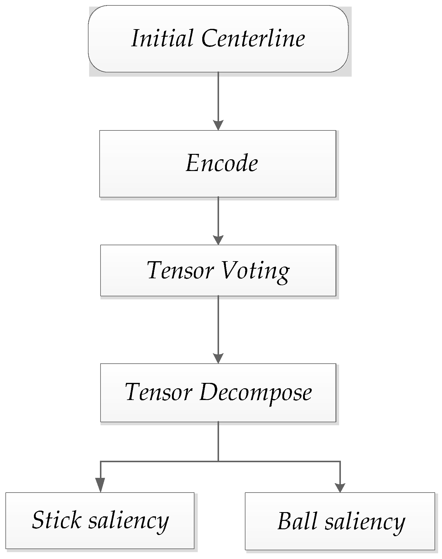
2. Methodology
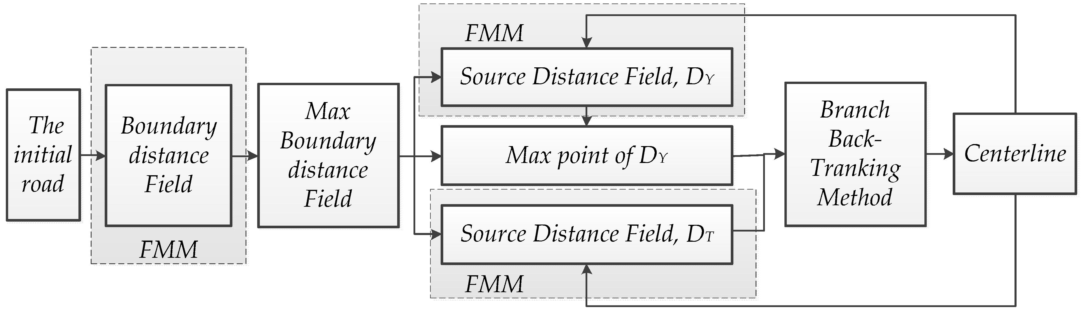
The proposed algorithms include (1) The preprocessing of the experimental data; (2) The initial road obtained by using multiscale segmentation and feature extraction; (3) The FMM used to obtain the boundary distance field and the source distance field, and the branch backing-tracking method used to get the initial centerline; (4) The road width of each centerline obtained by utilizing the boundary distance field and the initial road; (5) The tensor field used to connect the broken centerlines to get the final centerline; (6) The final centerline matched with its path width, and the final road reconstructed. The flowchart of this algorithm is shown in Figure 1.
2.1. Multiscale Segmentation and Feature Extraction
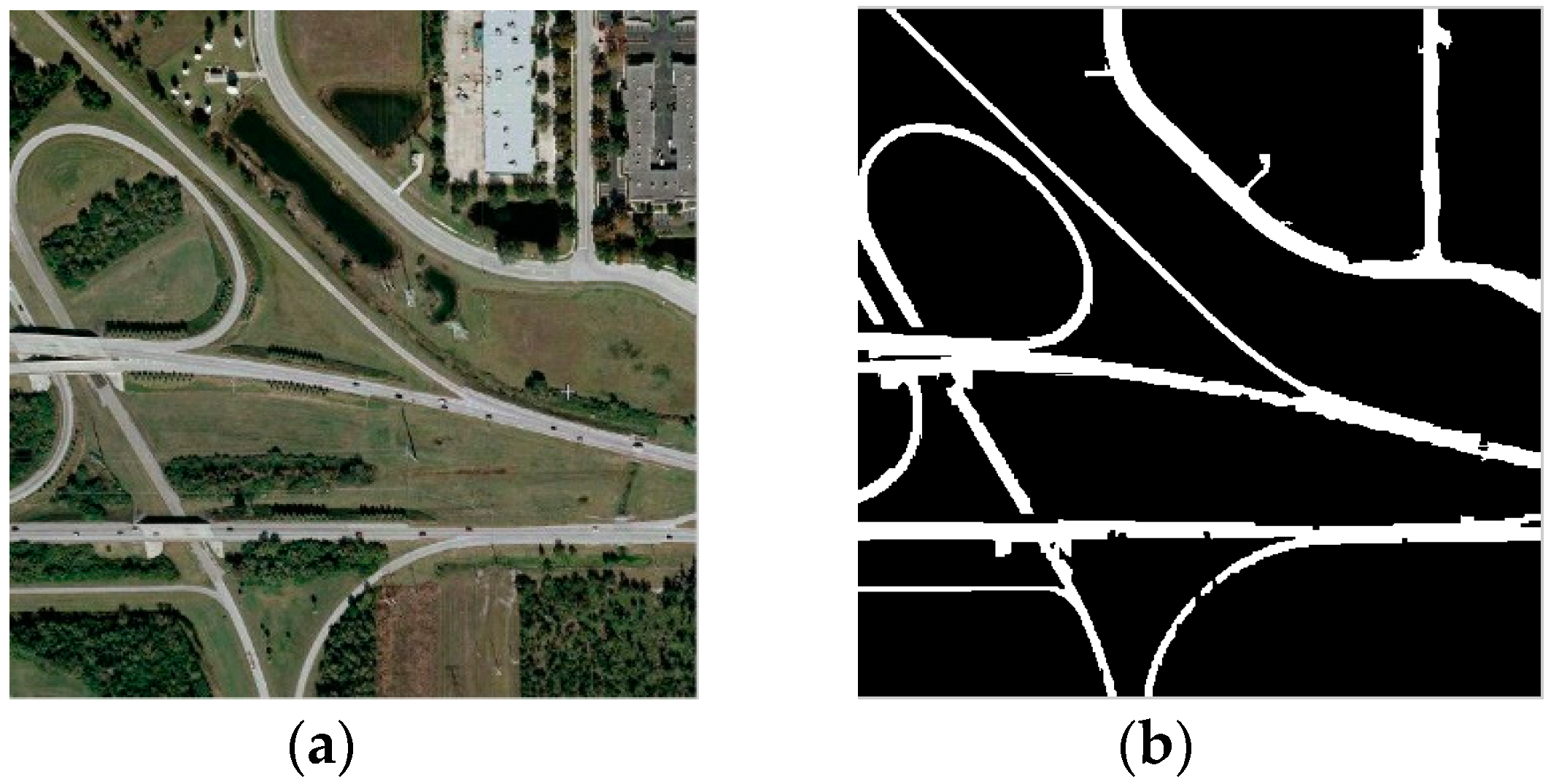
Though the high-resolution remote sensing image has rich band information, previous algorithms often made use of the image gray when using the high-resolution remote sensing image, which results in the rich spectral information not being fully exploited. This paper uses statistical region merging (SRM) [31] multiscale segmentation algorithm to segment the image, which not only fully utilizes the spectral features of high-resolution remote sensing images, but also guarantees the integrity of the image by choosing the proper segmentation scale. After the multiscale segmentation, according to the statistical analysis of road characteristics, we know that the road is generally continuous, and the surface radiation characteristics are consistent, and have a big length and width ratio value. On the basis of multiscale segmentation, a binary image is obtained by setting a specific threshold range on the multiscale segmentation result. The road area and aspect ratio feature are used to remove the non-road interference. Considering that the road is a continuous area and the road generally occupies a large proportion of the overall image, we can set the area parameters to eliminate the small area of non-road interference. In addition, according to the shape characteristics of the road, the road is generally slender, then we set the length–width ratio of the road greater than 1.5 to remove the large non-road area interference. The result of initial road extraction is shown in Figure 2.
2.2. The Extraction of Centerline
Skeleton extraction refers to the topological structure of a two-dimensional or three-dimensional object with a one-dimensional connected centerline, and the centerline of the road can be extracted by extracting the skeleton of the road [27]. On the basis of the acquired initial road from Section 2.1, this paper uses FMM to obtain the boundary distance field and the source distance field, and uses the minimum cost path algorithm to obtain the initialization centerline, as shown in Figure 3.
2.2.1. Obtaining Distance Field Using FMM Algorithm
Fast marching method (FMM) was introduced by Sethian [33,34] for a special case of front evolution. In this paper, the FMM algorithm is used to obtain the boundary distance field and the source distance field. Considering an interface (that is, the boundary of road or the maximum value point of the boundary in this paper), can be a point, a curve or a surface. Consider the case of a front moving with speed F(x), where F is always either positive or negative. Then, let be the time at which crosses the point x. In the one-dimensional case, where distance = speed time, the equation of motion can be expressed as
In multiple dimensions, the equation of evolution is:
where represents the speed when passes by the point x, represents the time gradient of crossing the point x, and indicates that the initial arrival time of is 0.
The process of solving the FMM algorithm is the process of obtaining . According to Equation (2), the only changing parameter is the speed function F(x). In this way, we can get a different T(x) by setting different speed functions. The initial position of the evolution curve and the speed of the evolution curve are the initial conditions of the curve evolution. We can understand the construction process of the distance field as follows: Γ evolves from the initial position in accordance with speed function F(x), continually, through all the pixels in the image. The cumulative time map of reached from all pixels is the desired distance field.
a. Calculating the boundary distance field D1
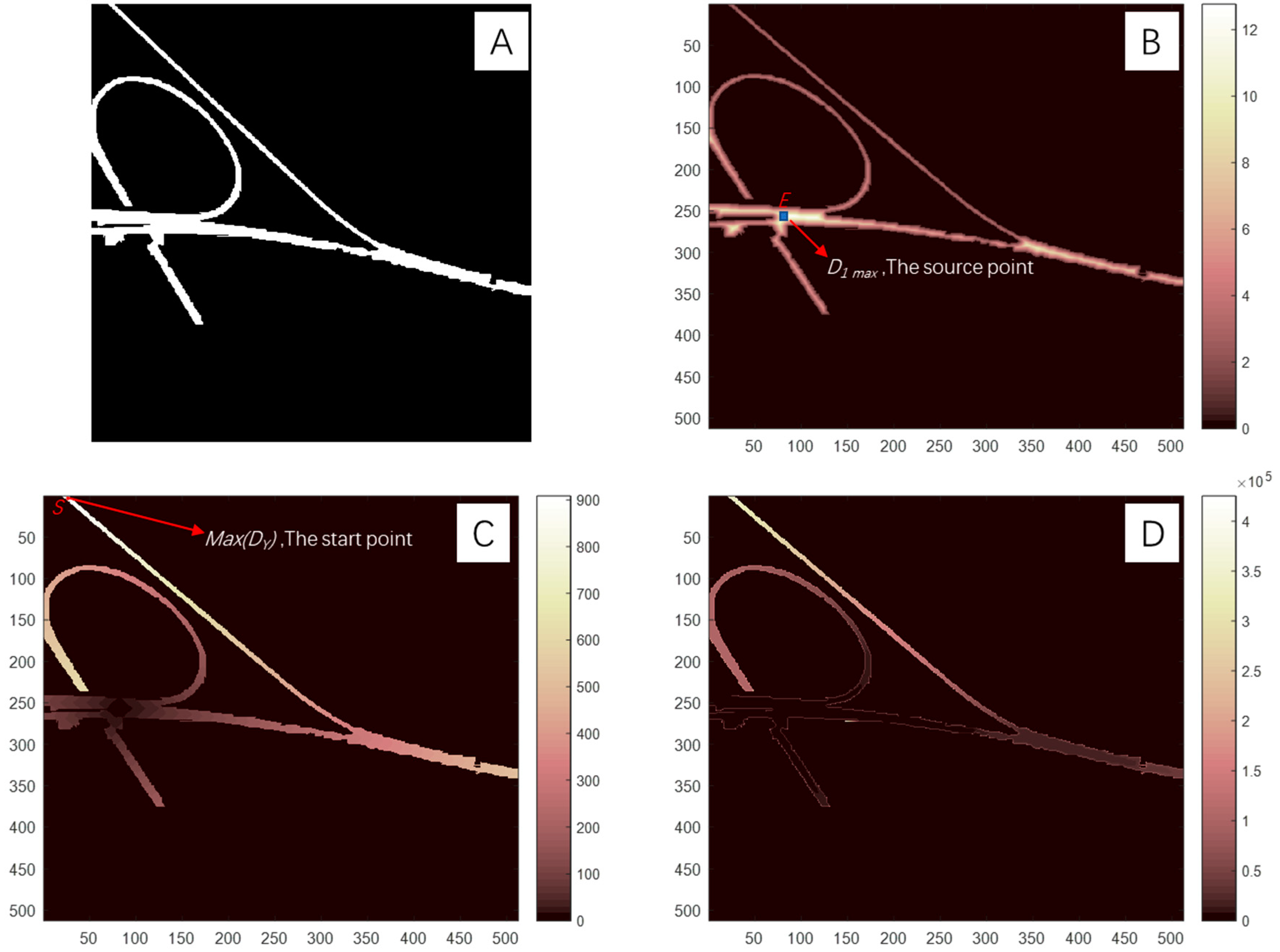
The boundary distance field D1 of the road describes the relative spatial distances between the pixels and the boundary. The outermost pixels of the road are used as the road boundaries and the pixels between boundaries are used as the road, because the road boundary occupies a pixel width, the width of the road is smaller than the actual value. As shown in Figure 4b, with q = 3 structural elements to dilate the road boundary (Figure 4c), the pixels occupied by the newly acquired boundary is only used as a road boundary and not as part of the road. The corresponding value at the road boundary in the boundary distance field D1 should be 0. When , is the Euclidean distance from the boundary to the current position, so a uniform speed function is defined as
where x is the spatial position of the pixel in the image, and is the speed at which the FMM evolves at that pixel. Substitute into Equation (2) to solve T(x) to obtain the boundary distance field D1.
b. Calculating the source distance field DY and DT for initial road
The source distance field records the spatial position relation from each pixel to the source point. On the basis of the boundary distance field D1, the maximum position of the boundary distance field E1 with the value is obtained, and the source distance fields DY and DT are obtained by using this point as the source point. The source point is the starting point of the source distance field calculation, which is the position of the zero-level set. The speed function of DY is defined the same as , so the DY records the Euclidean distance from each point to the source point. The speed function of DT is :
where is boundary distance field, and Dmax is the maximum value of the boundary distance field. According to the definition of boundary distance field, the nearer to the centerline, the larger is. Hence, has a greater value while near the centerline, that is, the nearer to the centerline, the faster the curve evolves and the smaller is. Figure 5 is a schematic diagram of the boundary distance field and source distance field, and we assume that Figure 5a is the initial road obtained by image segmentation. For the road boundary from Figure 5a, the evolution is performed at , and the boundary distance field can be obtained by masking the area outside the road, as shown in Figure 5b. For the maximum distance point E of the boundary distance field, the evolution is performed at , and the area outside the road is masked to obtain the source distance field DY, as shown in Figure 5c. The source point E evolves with speed function , and the area outside the road is masked to obtain the source distance field DY, as shown in Figure 5d.
2.2.2. Centerline Extraction Based on Branch Backing-Tracking Method
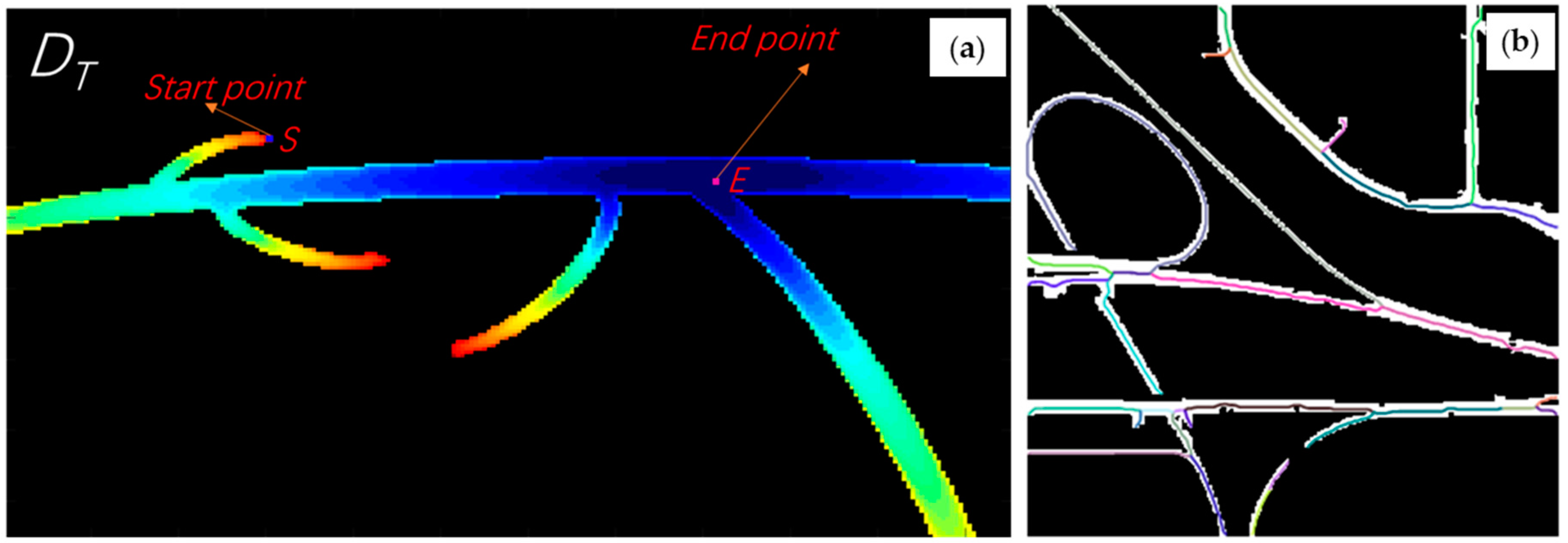
The maximum point S of the source distance field DY is selected as the starting point, and the maximum value point E of the boundary distance field is chosen as the end point, and the QSE is defined as all paths from the starting point S to end point E. Then, a branch backing-tracking method [18,25] is used for back-tracking the minimum cost path from the starting point S to the end point E on the source distance field DT, which is the centerline, as shown in Figure 6.
From the given start point S to the end point E, a minimum cost path Q(t) can be found: [0,∞]→Rn, where the cumulative cost function is the function of the pixel position x, and the minimum cumulative cost is defined as
where L is the cumulative distance (arrival time) from the starting point S along Q to the end point E; is the set of all possible paths from the starting point S to x; , as a cost function, is defined as ; and has a lower cost nearer the centerline and a higher cost away from the centerline, from which we can find the centerline of the road by finding the minimum value.
The extraction of centerline is the solution of the ordinary differential Equation (6).
where Q(t) is the centerline, and E is the farthest point. From the starting point S to the end point E, the minimum-cost back-tracking path is the centerline. For the current location Qx, the next location point Qx+1 is
where Qx+1 is the next point; is the local gradient of the current position; and w is the step. The smaller w is, the higher the accuracy of the centerline, here, 0.01 is often chosen as the step.
Then, the source distance field DY and DT are obtained by using the centerline Q(t) as the source.
After the acquisition of the new source distance field, the starting point S and end point E are selected as the same way above, then, the branch backing-tracking method is used to obtain the centerline and looped until all the centerline is found. In this way, the initialization centerline C1 is obtained, and the centerline is shown as in Figure 6b.
2.3. Road Width Extraction
As one of the key parameters of road extraction, road width is often neglected in previous studies. Due to the influence caused by vegetation, building shadows near roads, and other disturbances, the completeness of roads will be missing. In addition, for the effect of the surface features whose materials are similar to the road, the extracted roads will be wider than the actual roads. Assuming that the missing part of the road and the added part of the road are stochastic, this paper uses the coordinates of the centerline and the Euclidean distance from the centerline to the road boundary, to calculate the width of the road for each point in the centerline. We know that the width of a road is consistent, so we calculate the average width of each road branch as the road width Dr.
From the previous section, the initial centerline C1 has been obtained in Section 2.2.2. As shown in Figure 7, the road is extracted from an image of 400 × 400 pixels, where Figure 7a is the boundary distance field, and the closer to the centerline position, the larger of the value of the boundary distance field is, and the maximum value acquired at the centerline position; Figure 7b is the contour line of Figure 7a. For any point on the centerline of the road, suppose the value of boundary distance field xw is the distance from this point to road boundary, then the road width is Dr = 2 xw. The definition of road width is shown in Figure 7c.
2.4. Obtaining the Tensor Field
Although all the centerlines in the initial road have been detected, there are still many broken places in the centerlines. From the original image, we can know this part of the fault is caused by shadow and the cover of vegetation. The phenomenon of shadow, vehicle, vegetation, and other occlusions in the road is ubiquitous, and it is impossible to compensate by the optimized segmentation algorithm, so the tensor field is introduced for the link of the broken centerline.
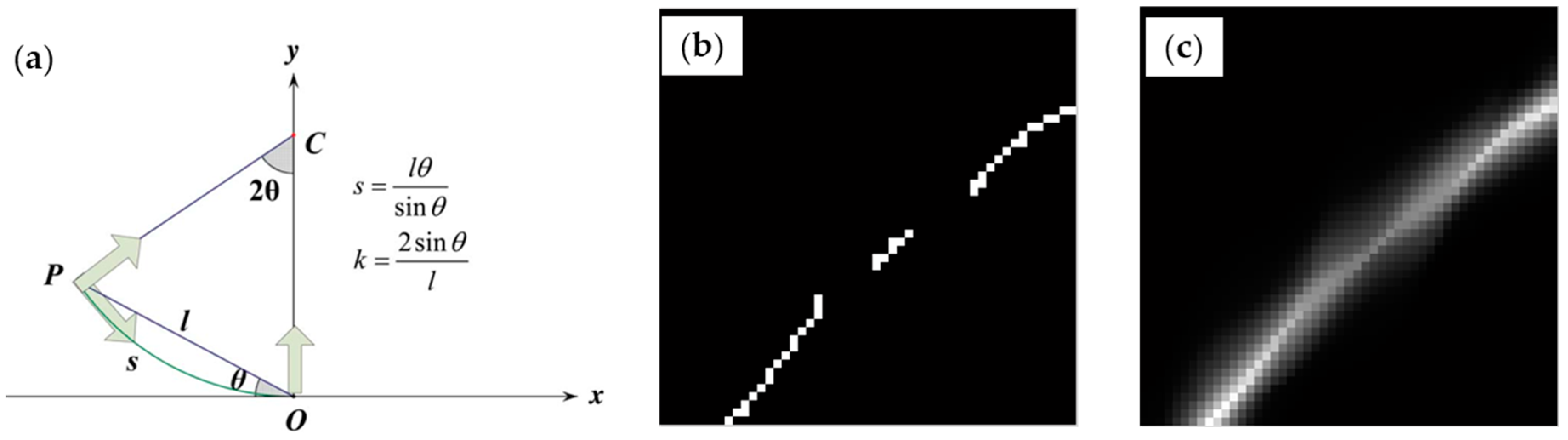
Tensor voting [35] is an algorithm that represents the saliency structure of an image, a method of reasoning its implied geometry from a large amount of unreliable information by passing (voting) tensor (differential geometric information) between adjacent points. In the algorithm, the neighborhood information is gathered together by the way of voting, and the orientation information is estimated by the calculation rules of the vector field. The flowchart for tensor voting is shown in Figure 8.
- (1)
- In the tensor encoding phase, the location information of the initialization centerline C1 is encoded as the initialization tensor T. For the initial centerline of the input (binary image): if the input pixel is a single pixel point, then the eigenvalues are l1 = l2 = 1, ; if the input pixel is a point on the curve and the normal vector of the point is , its eigenvalues are l1 = 1, l2 = 0, . According to the definition of matrix theory, any one second-order semidefinite tensor can be decomposed into two eigenvalues and two eigenvectors. The tensor T can be decomposed as follows:where e1 and e2 are eigenvectors, l1 and l2 are eigenvalues, , is the stick tensor, (l1 − l2) is the saliency of stick tensor; is the ball tensor; and l2 is the saliency of ball tensor.
- (2)
- Tensor voting is carried out on the initial tensor after encoding, and tensors communicate their information with each other in a neighborhood. A tensor vote is first made on the initialization tensor obtained from 1).The tensor field is expressed by the attenuation function DF. As shown in Figure 9a, we assume that O and P are two points in T, where O is the voting point and P is the receiving point, then, the voting intensity DF of P received from O point is as shown in Equation (9).where s is the osculating circle arc length of the voting center point to the voting point; k is the curvature of the osculating circle; is the size of the voting window; and c is a constant. The value of the voting window is determined by the size of the centerline fracture, and, if the fracture is large, then takes a relatively large value; here, it takes a value of 18.25. Where c is the constant associated with σ, the equation is .
- (3)
- Each point in the encoded initial centerline C1 votes to the point neighborhood within its tensor field, and accepts other points to vote for itself, getting a new tensor field TS.
- (4)
- After the voting, each point on the centerline has a new tensor field, and Equation (10) is used to decompose the tensor field TS. After decomposition, we can get the stick tensor saliency map and the ball tensor saliency map . Here, a stick tensor saliency map is used as boundary distance field in the centerline extraction process, and the new boundary distance field is called D3. In consideration of the fact that D3 is decaying without boundary, here, we set the value of the positions in D3 less than 0.3 to 0, and the value of about 0.3 indicates that the tensor field of the point is very small and negligible. The effect of tensor voting is shown in Figure 9c.
2.5. Final Centerline Extraction and Road Reconstruction
From Section 2.2, we know that the boundary distance field is a Euclidean distance field, which is used as the input of the initial centerline extraction. However, the distance field is faulty because of the segmentation algorithm and the condition of the road itself. The D3 obtained in Section 2.3 is similar to the boundary distance field D1, that is, the pixels closer the centerline have higher values. Thus, the boundary distance field D3, acquired in the Section 2.4, is used to extract the final centerline, and the speed function is redefined as
where D3 is the boundary distance field, and is the maximum value of D3.
After that, we look for the maximum point E2 for D3, and redo the processes in Section 2.2.1(b) and Section 2.2.2. With the source distance field DY and DT updating constantly and centerline merging continuously, we get the final centerline C2, which is connected in the broken.
As shown in Figure 10b,c, the distances from different branches of the initial centerline C1 to C2 are calculated, and the road of the branch centerline with the minimum distance is selected as the road width of C2. For all the final connected centerlines in the road network, according to the final centerline, the C2 position matches the initial centerline C1 position and the corresponding road width Dr. Here, the broken road width the in C1 obtained from the surrounding road width. Through widening final centerline C2 to the corresponding road width Dr, the complete road W is obtained, and the complete road information extraction is realized.
3. Results
3.1. Experiment
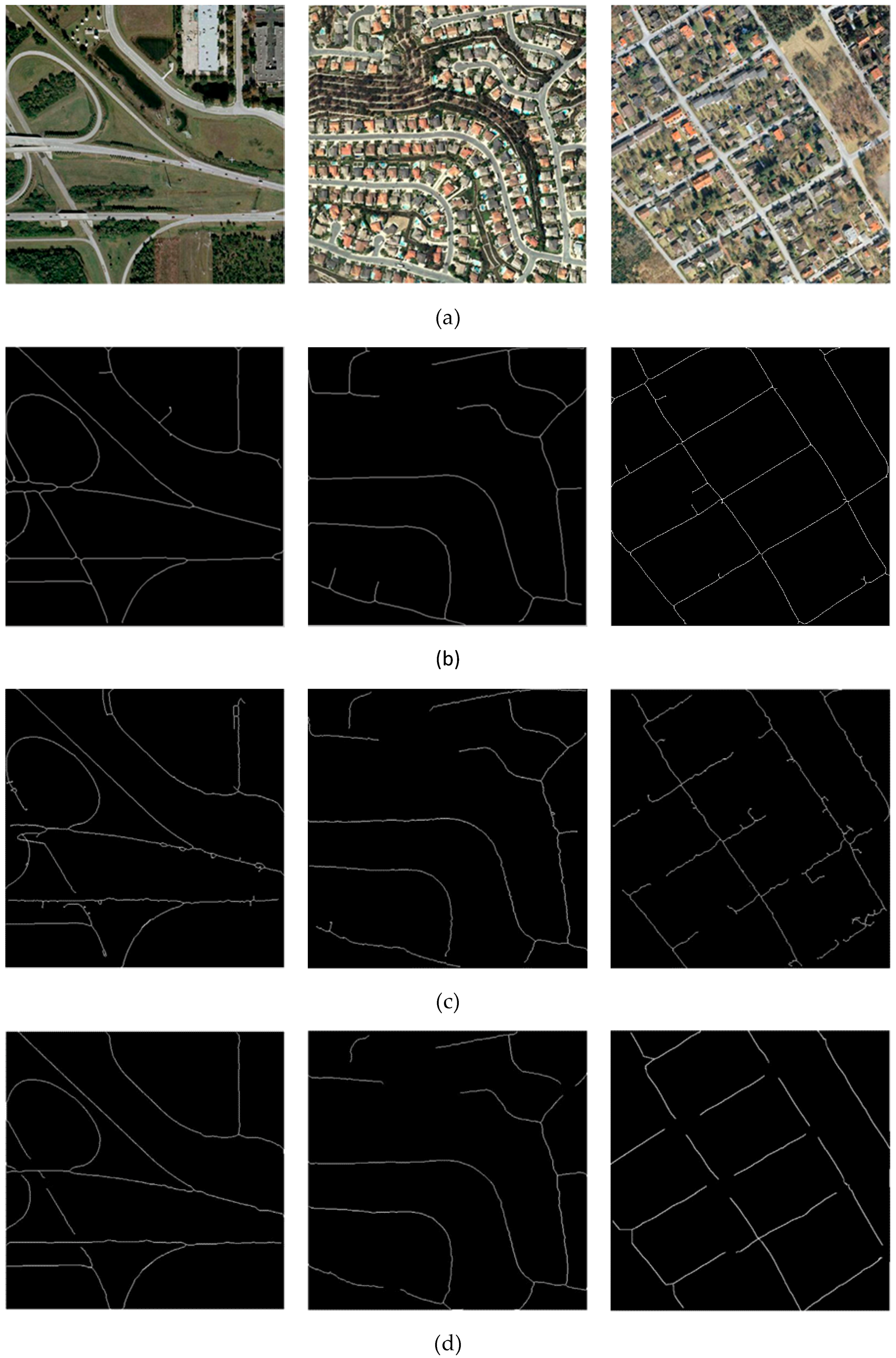
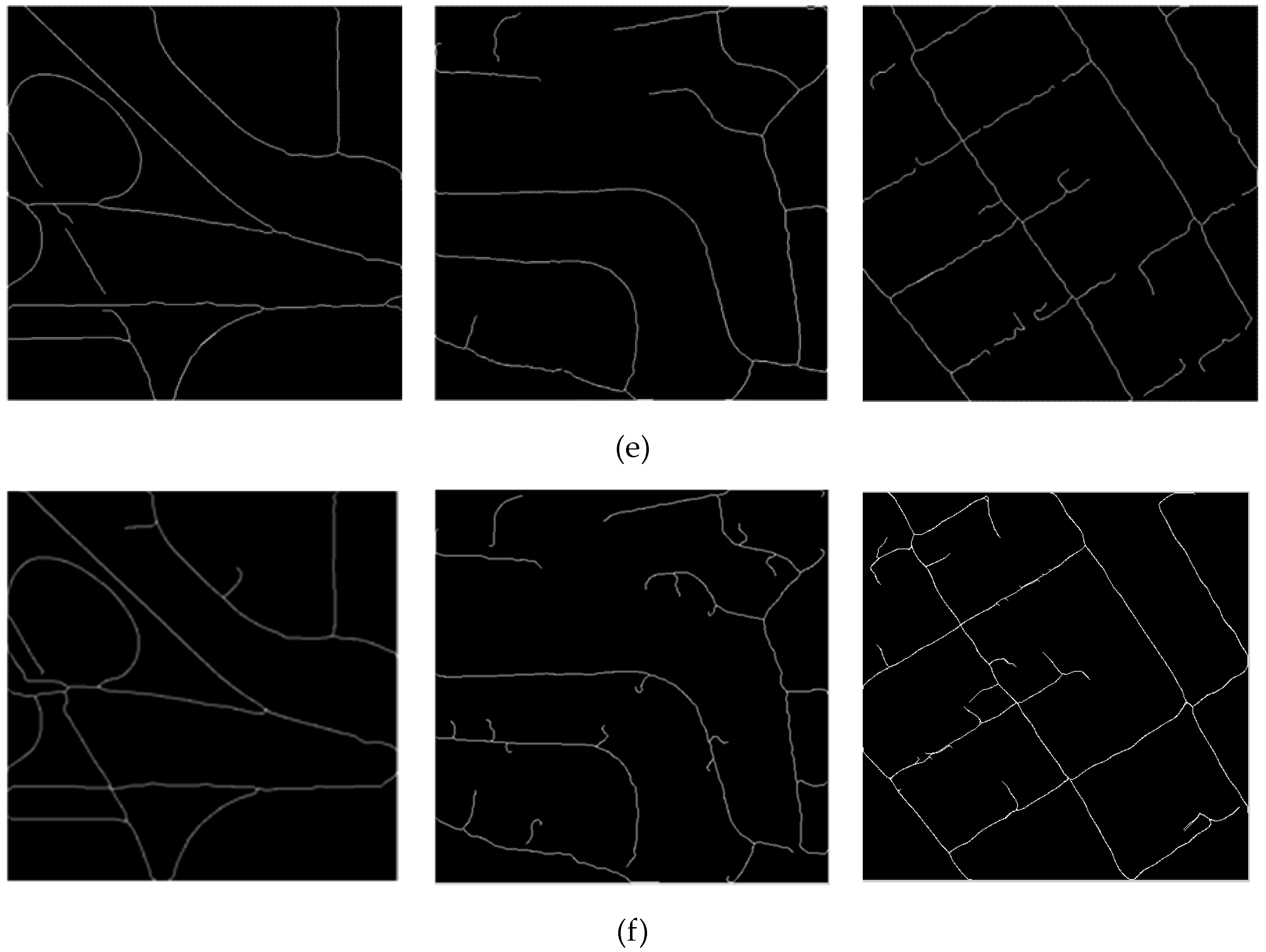
Three sets of data from difference part of urban are selected in order to demonstrate the validity of the proposed algorithm, which are all from the website http://www.cse.iitm.ac.in/~vplab/satellite.html. In order to make the proposed method better used in urban regional scale road extraction, this paper selects urban images under different circumstances to extract the road. The data are QuickBird images fused by panchromatic and multispectral images, whose sizes are all 512 × 512 pixels with a resolution of 0.61 m. The experimental results are shown in Figure 11, Figure 12 and Figure 13, where (a) is the picture fused by panchromatic and multispectral images; (b) is the initial road, which is extracted by SRM multiscale segmentation and feature extraction; (c) is the initial centerline, in which the broken centerlines are marked with red rectangles; (d) is the tensor field obtained by the initial centerline; (e) is the complete centerline after the connection, with an unconnected broken centerline marked with red rectangle; and (f) is the extracted road, which is reconstructed by the final centerline and road width.
3.1.1. Experiment on Image 1
For image 1, the road is in the field, and the road widths are from various different sources. Several sites of the roads are affected by the overpass shadows, and some are obscured by vegetation. The roads and centerlines in Figure 11b,c are broken by the shadows and vegetation. By the utilization of tensor voting, the broken centerlines are well connected. As shown in Figure 11e, the breakage in the red rectangle is too large to be connected.
3.1.2. Experiment on Image 2
For the image 2, the road is in a residential area. The materials on the main road and several examples of landcover before the buildings are the same, which causes great confusion for road extraction. In addition, there are other road materials at the junctions, which easily leads to road breakage. As shown in Figure 12b, many non-road features have been misjudged as roads, due to the disturbance of the landcover with the same materials as the road. As shown in Figure 12c–e, the broken centerlines are all connected, which greatly improves the integrity of the road extraction.
3.1.3. Experiment on Image 3
For image 3, the road is located between a residential area’s wastelands. On the way to the house, there are similar small paths which are characterized as the same as the road. This experiment treats these paths as roads. Many parts of the road are disturbed by the shading of vegetation and buildings, as shown in Figure 13a, which results in 12 breakages, nine of which are connected by tensor voting.
3.2. Analysis of Centerline Extraction Results
The manual drawing method is used to obtain reference road and reference centerline in order to evaluate the quality of the road extraction algorithm. The reference data are shown in Figure 14.
For the centerline, the centerline appraisal method proposed by Wiedemmann et al. [36] is used to evaluate the centerline result. The equations are as follows:
where Com, Cor, and Q represent completeness, correct, and quality, respectively. TP is the number of pixels both in the centerline and the reference centerline; FP is the number of pixels in the centerline but not in the reference centerline; and FN is the number of pixels in the reference centerline but not in the centerline. The number of TP, FP, and FN obtained from our method are exhibited in Table 1.
Based on the experimental results of the four methods in Table 2, we can know the Com, Cor, and Q of our algorithm for road centerline extraction are all higher than those of the previous three algorithms. According to the data statistics in Table 1, FP is always greater than FN because the tensor voting can solve, well, the faults of the centerline, and greatly improve the precision of centerline extraction. However, the tensor voting algorithm also extends the centerline at the end of road, allowing the centerline to be greater than its actual value at the end, which also results in the completeness always being less than the accuracy.
3.3. Analysis of Road Width Extraction Results
Ten samples are randomly selected for road width statistics on the reference road, as shown in Figure 15, so as to verify the accuracy of the extracted road width. With the purpose of ensuring the representativeness of the selected road width samples, the road width of three positions are measured separately, and the average value of the three positions is utilized as the reference road width. Then, the reference road widths are compared with the road widths, as shown in Figure 11f, and the width data statistics are displayed in Table 3, where the mean absolute error of the road width is 4.324%, and the average accuracy of the road width is 95.676%. The effective extraction of road width demonstrates that the proposed algorithm can extract complete road information well.
4. Discussion
4.1. Significance of Road Extraction Based on Remote Sensing Image
The proposed research focuses on the accurate extraction of road centerline and road width. As a main feature in urban construction, roads, with their rational planning and construction, are of great significance to urban development. The traditional method of road information collection is mainly carried out by manual means, where the road information is updated slowly and consumes enormous human physical and financial resources. Nowadays, the rapid development of satellites and the birth of satellite remote sensing images, with a resolution better than 1 m, provide the possibility to use remote sensing images for road extraction, and the remote sensing images for road extraction has the advantages of timely information, wide range, and low cost, compared with traditional methods of road information collection.
For example, the City Prosperity Index (CPI) is an important data for sustainable development analysis [37,38,39]. Here, roads are an important indicator for the CPI, especially in the following aspects [40]:
- Economic Density: Economic density is the city product [41] divided by the city’s area, its definition is as follows: , Where city square kilometer includes: residential and non-residential buildings, major roads, railways, and sport facilities. Here, the proposed road extraction method can be used to calculate the area of the road within square kilometers effectively.
- Population Density [42]. High-density neighborhoods tend to decrease the costs of public services. So, a reasonable urban planning of high population density is the key to determine urban sustainable development, which includes: police and emergency response, school transport, roads, water and sewage, etc.
- Street Intersection Density. It means number of street intersections per one square kilometer of urban area. In order to calculate this index, we need to: Obtain the street network map of the urban area; Verify the topology: each street segment must be properly connected to other segments; Obtain the start and end point of each segment; Collect events from start and end points; Exclude points with less than 3 events; Count the remaining points and divide by the urban area in km2. For the above information, the method of getting road network is the key technique. Using the proposed road extraction, can efficiently obtain the urban road network information and road details, to provide data support for the street intersection density.
- Street Density. Number of kilometers of urban streets per square kilometer of land which is defined as: . The proposed algorithm can obtain the high precision road centerline, we can obtain the city street length through computing centerline length. In this way, the street density can be obtained effectively.
- Land Allocated to Streets. Land allocated to streets means total area of urban surface allocated to streets. It was defined as: . Here, we propose a road extraction algorithm that can directly carry out Road area statistics and get total surface of urban streets.
Remote sensing image road extraction method is not only an important measure for UN-Habitat to measure the sustainable development of urban, it also plays a very important role in people’s daily life. Construction of smart cities makes the efficient road extraction method an urgent need. According to the wide range of remote sensing images, we can use the high-resolution remote sensing images to:
- Update the GPS system information timely. Road is one of the most important information of GPS, the use of road extraction from high-resolution remote sensing image can update GPS information timely.
- Conduct traffic situation assessment. According to the distribution of road and vehicle to figure out the congestion of road, not only to provide owners with the best travel program but also greatly improve the efficiency of traffic management.
- Prepare statistics for urban road distribution and land consumption rates, so as to facilitate urban planning. Road and building are the two most important components of urban. Recently, the global population is growing rapidly, taking up more and more resources on the earth, and remote sensing image road extraction can be used in statistics for the distribution of urban roads, and contribute to the rational planning and sustainable development of cities.
- Evaluate the urban population density and urban economic growth based on road development. The intensity of road network is positively correlated with the degree of urban population and economic development. The use of road statistics can establish population density and economic development models, used to assess the comprehensive strength of urban development.
- Implement urban change monitoring. Remote sensing images keep the historical data of the city well, analyze the road information obtained from remote sensing images at different times, and can analyze the changing trends of urban development effectively.
4.2. Comparison of the Methods for Centerline Extraction
Previous studies [2,3,4,5,6] have shown that the high-resolution remote sensing imagery for road extraction still has many problems. Unlike the remote sensing imagery with rich spectral information, traditional image segmentation algorithms tend to only consider the information of single bands, which are difficult for guaranteeing the accuracy of image segmentation. In addition, due to the vegetation shading, building shadows, and other effects, it is easy to cause centerline fractures and incomplete road surfaces. In view of these problems, this study does its work from three aspects: using the multiscale segmentation algorithm to enhance the accuracy of image segmentation; employing the tensor voting algorithm to connect broken centerlines; and combining road width and centerline to reconstruct roads.
In Figure 10c–e, Figure 11c–e, and Figure 12c–e, the tensor vote algorithm was applied for connecting broken centerlines. However, for large centerline fractures, such as the red rectangles in Figure 10e and Figure 12e, the algorithm was still unable to connect the broken centerlines. This study used Com, Cor, and Q to evaluate the extracted centerline. The Experiment 1 showed high values of Com, Cor, and Q, whereas Experiment 2 had mistaken some non-road areas as roads, resulting in Com less than Cor, but all three indicators were above 90%. The background of the Experiment 3 data was more complex, because, during the initial road extraction, there was an unextracted road, due to the disturbance of the vegetation shading, which resulted in lower Com and Q.
In the previous study of road extraction algorithms [10,17,29], many scholars had studied the extraction of road centerline. In order to fully verify the superiority of this algorithm, the centerline algorithm was compared with Ruyi Liu’s algorithm [17], Chaudhuri’s [10] algorithm, and Shi’s [29] algorithm. In Chaudhuri’s method, Chaudhuri segmented the enhanced image and obtained the road by the artificial template with small noise removed. Finally, the road centerline was obtained through morphological thinning. In Shi’s method, Shi obtained the initial road based on the spectral-spatial classification result, and fused the road groups and homogeneous property to improve road-group accuracy. Then, the local linear kernel smoothing regression algorithm was used to obtain the centerline of road after a morphological processing. In Ruyi Liu’s method, initial road regions were obtained by combining the shear transform algorithm with directional segmentation. Then, the road map based on Mahalanobis distance and thresholding was fused with the initial road regions to improve accuracy. Finally, the road centerline was extracted by the skeleton algorithm proposed by Uitert and Bitter.
The comparison results are shown in Figure 16, where (a) is the experimental data; (b) is the reference centerline extracted manually; (c) is the centerline extracted by the Chaudhuri’s method; (d) is the centerline by the Shi’s method; (e) is the centerline by the Ruyi Liu’s method; and (f) is the centerline by the proposed algorithm.
Compared with the other three algorithms, this method used the tensor voting algorithm to connect the broken centerline, as shown in Figure 15, which greatly improves the completeness of the centerline. The results of the evaluation are exhibited in Table 4 where the completeness, correctness, and quality of the proposed algorithm are much better than those of the previous three algorithms.
4.3. Assessment of Road Width Extraction
Based on the accurate extraction of the centerline, the paper studied the road width extraction and received a good result. In this study, the distance from each point on the centerline to the edge of the road was calculated to find the road width. The road width was replaced by the average of each section of road width according to the continuity of the road. For the road width extraction, ten samples were selected randomly in Section 3.3, and the calculated road width and the road width on the reference road were compared and analyzed. As shown in Table 3, the average accuracy of road width extraction was as high as 95.676%, which indicates that the method of using centerline and road width for reconstruction is appropriate.
In general, the proposed method improves the accuracy of the centerline extraction, and the method can extract the road width accurately. Using the centerline and road width to reconstruct roads can solve, well, the problem of incomplete road extraction caused by shading.
5. Conclusions
A new method of road extraction is presented in this paper, where the multiscale segmentation algorithm makes full use of the spectral information in high-resolution remote sensing images. Using the tensor voting algorithm to connect fault centerlines greatly improves the integrity of centerline. The method of reconstructing roads with road width and centerline information solves the problem that the road integrity is affected by vegetation and shadows.
To verify the effectiveness of the proposed algorithm, three QuickBird images were tested. Parameters of completeness, correctness, and quality were used to evaluate the centerline extraction results. In addition, we compared the centerline extraction results with the other three centerline extraction algorithms. The comparison results show that the introduction of the tensor voting algorithm solves the problem of broken centerline effectively. For road width, ten samples were selected on the road, with the comparison between the extracted road width and the road width on the reference data. The analysis results demonstrate that the average extraction accuracy of the road width is 95.68%.
In future work, we will enhance the segmentation algorithm to improve segmentation accuracy, study shadow removal algorithms to reduce road extraction interference, and improve the algorithms of broken centerline connection. Characteristics of roads on multispectral and hyperspectral images will also be attached with great importance, by using spectral features to improve road extraction accuracy.
Author Contributions
Conceptualization of the experiments: T.Z., H.F. and C.S.; Data curation: T.Z.; Methodology: T.Z., and H.F.; Funding acquisition: C.S.; Data analysis: T.Z.; Writing—original draft preparation: T.Z.; Writing—review and editing: H.F. and C.S.; Supervision: H.F. and C.S.
Funding
This research received no external funding.
Acknowledgments
The authors would like to thank the editors end reviewers for their suggestions and revisions. The authors are also highly grateful for the help from the excellent translator (Yun Nie).
Conflicts of Interest
The authors declare no conflict of interest.
References
- Wang, W.; Yang, N.; Zhang, Y.; Wang, F.; Cao, T.; Eklund, P. A review of road extraction from remote sensing images. J. Traffic Transp. Eng. Engl. Ed. 2016, 3, 271–282. [Google Scholar] [CrossRef] [Green Version]
- Steger, C.; Glock, C.; Eckstein, W.; Mayer, H.; Rading, B. Model-based road extraction from images. In Automatic Extraction of Man-Made Objects from Aerial and Space Images; Springer: Berlin/Heidelberg, Germany, 1995; pp. 275–284. [Google Scholar]
- Koutaki, G.; Uchimura, K. Automatic road extraction based on cross detection in suburb. In Proceedings of the Computational Imaging II, Anaheim, CA, USA, 9–10 April 2017; pp. 337–345. [Google Scholar]
- Zhang, C.; Baltsavias, E.P.; Gruen, A. Knowledge-Based Image Analysis for 3D Road Reconstruction; ETH Zurich Institute of Geodesy and Photogrammetry: ETH Hönggerberg, Switzerland, 2001; pp. 3–14. [Google Scholar] [CrossRef]
- Zhang, C.; Murai, S.; Baltsavias, E.P. Road network detection by mathematical morphology. In Proceedings of the ISPRS Workshop 3D Geospatial Data Production: Meeting Application Requirements, Paris, France, 7–9 April 1999. [Google Scholar]
- Baumgartner, A.; Steger, C.T.; Mayer, H.; Eckstein, W. Semantic objects and context for finding roads. In Proceedings of the Integrating Photogrammetric Techniques with Scene Analysis and Machine Vision III, Orlando, FL, USA, 21–23 April 1997; pp. 98–110. [Google Scholar]
- Vosselman, G.; De Knecht, J. Road tracing by profile matching and Kaiman filtering. In Automatic Extraction of Man-Made Objects from Aerial and Space Images; Springer: Berlin/Heidelberg, Germany, 1995; pp. 265–274. [Google Scholar]
- Changqing, Z.; Yun, Y.; Fang, Z.; Qisheng, W. Total rectangle matching approach to road extraction from high resolution remote sensing images. J. Huazhong Univ. Sci. Technol. Nat. Sci. Ed. 2008, 36, 74–77. [Google Scholar] [CrossRef]
- Park, S.-R.; Kim, T. Semi-automatic road extraction algorithm from IKONOS images using template matching. In Proceedings of the 22nd Asian Conference on Remote Sensing, Singapore, 5–9 November 2001; p. 9. [Google Scholar]
- Chaudhuri, D.; Kushwaha, N.; Samal, A. Semi-automated road detection from high resolution satellite images by directional morphological enhancement and segmentation techniques. IEEE J. Sel. Top. Appl. Eearth Obs. Remote Sen. 2012, 5, 1538–1544. [Google Scholar] [CrossRef]
- Nevatia, R.; Babu, K.R. Linear feature extraction and description. Comput. Graph. Image Process. 1980, 13, 257–269. [Google Scholar] [CrossRef]
- Fua, P.; Leclerc, Y.G. Model driven edge detection. Mach. Vis. Appl. 1990, 3, 45–56. [Google Scholar] [CrossRef] [Green Version]
- Neuenschwander, W.M.; Fua, P.; Iverson, L.; Székely, G.; Kübler, O. Ziplock snakes. Int. J. Comput. Vis. 1997, 25, 191–201. [Google Scholar] [CrossRef]
- Marikhu, R.; Dailey, M.N.; Makhanov, S.; Honda, K. A family of quadratic snakes for road extraction. In Proceedings of the Asian Conference on Computer Vision, Tokyo, Japan, 18–22 November 2007; pp. 85–94. [Google Scholar]
- Miao, Z.; Wang, B.; Shi, W.; Zhang, H. A semi-automatic method for road centerline extraction from VHR images. IEEE Geosci. Remote Sens. Lett. 2014, 11, 1856–1860. [Google Scholar] [CrossRef]
- Miao, Z.; Wang, B.; Shi, W.; Wu, H.; Wan, Y. Use of GMM and SCMS for accurate road centerline extraction from the classified image. J. Sens. 2015, 2015, 1–13. [Google Scholar] [CrossRef]
- Liu, R.; Miao, Q.; Huang, B.; Song, J.; Debayle, J. Improved road centerlines extraction in high-resolution remote sensing images using shear transform, directional morphological filtering and enhanced broken lines connection. J. Vis. Commun. Image Represent. 2016, 40, 300–311. [Google Scholar] [CrossRef]
- Van Uitert, R.; Bitter, I. Subvoxel precise skeletons of volumetric data based on fast marching methods. Med. Phys. 2007, 34, 627–638. [Google Scholar] [CrossRef]
- Huang, X.; Zhang, L. Road centreline extraction from high-resolution imagery based on multiscale structural features and support vector machines. Int. J. Remote Sens. 2009, 30, 1977–1987. [Google Scholar] [CrossRef]
- Cheng, G.; Zhu, F.; Xiang, S.; Wang, Y.; Pan, C. Accurate urban road centerline extraction from VHR imagery via multiscale segmentation and tensor voting. Neurocomputing 2016, 205, 407–420. [Google Scholar] [CrossRef] [Green Version]
- Otsu, N. A threshold selection method from gray-level histograms. IEEE Trans. Syst. Cybern. 1979, 9, 62–66. [Google Scholar] [CrossRef]
- Bezdek, J.C.; Ehrlich, R.; Full, W. FCM: The fuzzy c-means clustering algorithm. Comput. Geosci. 1984, 10, 191–203. [Google Scholar] [CrossRef]
- Wagstaff, K.; Cardie, C.; Rogers, S.; Schrödl, S. Constrained k-means clustering with background knowledge. In Proceedings of the ICML, Williamstown, MA, USA, 28 June–1 July 2001; pp. 577–584. [Google Scholar]
- Bieniek, A.; Moga, A. An efficient watershed algorithm based on connected components. Pattern Eecognit. 2000, 33, 907–916. [Google Scholar] [CrossRef]
- Gao, L.; Shi, W.; Miao, Z.; Lv, Z. Method based on edge constraint and fast marching for road centerline extraction from very high-resolution remote sensing images. Remote Sens. 2018, 10, 900. [Google Scholar] [CrossRef]
- Osher, S.; Sethian, J.A. Fronts propagating with curvature-dependent speed: algorithms based on Hamilton-Jacobi formulations. J. Comput. Phys. 1988, 79, 12–49. [Google Scholar] [CrossRef]
- Sethian, J.A. A fast marching level set method for monotonically advancing fronts. Proc. Natl. Acad. Sci. USA 1996, 93, 1591–1595. [Google Scholar] [CrossRef] [PubMed]
- Malladi, R.; Sethian, J.A. An O (N log N) algorithm for shape modeling. Proc. Natl. Acad. Sci. USA 1996, 93, 9389–9392. [Google Scholar] [CrossRef] [PubMed]
- Zhang, Y.; Zhang, J.; Li, T.; Sun, K. Road extraction and intersection detection based on tensor voting. In Proceedings of the 2016 IEEE International Geoscience and Remote Sensing Symposium (IGARSS), Beijing, China, 10–15 July 2016; pp. 1587–1590. [Google Scholar]
- Shi, W.; Miao, Z.; Debayle, J. An integrated method for urban main-road centerline extraction from optical remotely sensed imagery. IEEE Trans. Geosci. Remote Sens. 2014, 52, 3359–3372. [Google Scholar] [CrossRef]
- Nock, R.; Nielsen, F. Statistical region merging. IEEE Trans. Pattern Anal. Mach. Intell. 2004, 26, 1452–1458. [Google Scholar] [CrossRef] [PubMed] [Green Version]
- Wu, T.-P.; Yeung, S.-K.; Jia, J.; Tang, C.-K.; Medioni, G. A Closed-Form Solution to Tensor Voting: Theory and Applications. IEEE Trans. Pattern Anal. Mach. Intell. 2012, 38, 1482–1495. [Google Scholar]
- Sethian, J.A. Fast marching methods. Siam Rev. 1999, 41, 199–235. [Google Scholar] [CrossRef]
- Hassouna, M.S.; Farag, A.A. Multistencils fast marching methods: A highly accurate solution to the eikonal equation on cartesian domains. IEEE Trans. Pattern Anal. Mach. Intell. 2007, 29, 1563–1574. [Google Scholar] [CrossRef] [PubMed]
- Christodoulidis, A.; Hurtut, T.; Tahar, H.B.; Cheriet, F. A multi-scale tensor voting approach for small retinal vessel segmentation in high resolution fundus images. Comput. Med. Imaging Graph. 2016, 52, 28–43. [Google Scholar] [CrossRef] [PubMed]
- Wiedemann, C.; Heipke, C.; Mayer, H.; Jamet, O. Empirical evaluation of automatically extracted road axes. In Empirical Evaluation Techniques in Computer Vision; Wiley-IEEE Computer Society Press: Washington, DC, USA, 1998; pp. 172–187. [Google Scholar]
- Marans, R.W. Quality of urban life & environmental sustainability studies: Future linkage opportunities. Habitat Int. 2015, 45, 47–52. [Google Scholar]
- Yigitcanlar, T.; Dur, F.; Dizdaroglu, D. Towards prosperous sustainable cities: A multiscalar urban sustainability assessment approach. Habitat Int. 2015, 45, 36–46. [Google Scholar] [CrossRef] [Green Version]
- Arbab, P. City Prosperity Initiative Index: Using AHP Method to Recalculate the Weights of Dimensions and Sub-Dimensions in Reference to Tehran Metropolis. Eur. J. Sustain. Dev. 2017, 6, 289–301. [Google Scholar] [CrossRef]
- MEASUREMENT OF CITY PROSPERITY: Methodology and Metadata. Available online: http://cpi.unhabitat.org/sites/default/files/resources/CPI%20METADATA.2016.pdf (accessed on 13 December 2018).
- Ciccone, A.; Hall, R.E. Productivity and the density of economic activity. Natl. Bureau Econ. Res. 1993, 86, 54–70. [Google Scholar] [CrossRef]
- Habitat, U. A New Strategy of Sustainable Neighbourhood Planning: Five Principles. United Nations Human Settlements Programme: Nairobi, Kenya, 2014. Available online: https://unhabitat.org/a-new-strategy-of-sustainable-neighbourhood-planning-five-principles/ (accessed on 13 December 2018).
Figure 1.
Flowchart of the proposed road information extraction based on road reconstruction.

Figure 2.
The extraction of initial road. (a) Original image; (b) Initial road after multiscale segmentation and feature extraction.
Figure 2.
The extraction of initial road. (a) Original image; (b) Initial road after multiscale segmentation and feature extraction.

Figure 3.
The extraction of centerline.

Figure 4.
The extraction of boundary distance field. (a) The boundary of initial road; (b) Local magnification image of the boundary, which shows a width of a pixel occupied by the boundary; (c) The values of boundary distance from (b).
Figure 4.
The extraction of boundary distance field. (a) The boundary of initial road; (b) Local magnification image of the boundary, which shows a width of a pixel occupied by the boundary; (c) The values of boundary distance from (b).

Figure 5.
(a) The initial road; (b) Boundary distance field of initial road, the point E has the maximum value of the boundary distance field with the value of and E is selected as the source point of DY and DT; (c) The source distance field DY with the speed function , the point S has the maximum value of DY and S is chosen as the start point in Section 2.2.2; (d) The source distance field DT with the speed function .

Figure 6.
Centerline extraction. (a) The schematic diagram [18] of the source distance field DT with the speed of —the darker pixels represent lower values, whereas the lighter indicates higher values; (b) The centerlines of different road branches shown in different colors.
Figure 6.
Centerline extraction. (a) The schematic diagram [18] of the source distance field DT with the speed of —the darker pixels represent lower values, whereas the lighter indicates higher values; (b) The centerlines of different road branches shown in different colors.

Figure 7.
(a) The boundary distance field of road; (b) The contour line of road; (c) The definition of road width; (d) The branch with difference road width.
Figure 7.
(a) The boundary distance field of road; (b) The contour line of road; (c) The definition of road width; (d) The branch with difference road width.

Figure 8.
Flowchart of tensor voting.

Figure 9.
Tensor voting. (a) Schematic diagram of tensor voting; (b) Broken centerline; (c) The result of tensor voting.
Figure 9.
Tensor voting. (a) Schematic diagram of tensor voting; (b) Broken centerline; (c) The result of tensor voting.

Figure 10.
Matching road width. (a) Initial centerline; (b) Initial centerline shown in the initial road, where C1a, C1b, and C1c are three different branches of initial road, and Dr1, Dr2, and Dr3 are the corresponding widths of the three branches; (c) The connected centerline, (c) The reconstructed road.

Figure 11.
Experiment 1 of QuickBird image. (a) Original image; (b) Initial road; (c) Initial centerline; (d) Tensor voting; (e) Final centerline; (f) Reconstructed road.
Figure 11.
Experiment 1 of QuickBird image. (a) Original image; (b) Initial road; (c) Initial centerline; (d) Tensor voting; (e) Final centerline; (f) Reconstructed road.


Figure 12.
Experiment 2 of QuickBird image. (a) Original image; (b) Initial road; (c) Initial centerline; (d) Tensor voting; (e) Final centerline; (f) Reconstructed road.
Figure 12.
Experiment 2 of QuickBird image. (a) Original image; (b) Initial road; (c) Initial centerline; (d) Tensor voting; (e) Final centerline; (f) Reconstructed road.

Figure 13.
Experiment 3 of QuickBird image. (a) Original image; (b) Initial road; (c) Initial centerline; (d) Tensor voting; (e) Final centerline; (f) Reconstructed road.
Figure 13.
Experiment 3 of QuickBird image. (a) Original image; (b) Initial road; (c) Initial centerline; (d) Tensor voting; (e) Final centerline; (f) Reconstructed road.

Figure 14.
Reference road and reference centerline. (a) Reference road of experiment 1; (b) Reference centerline of experiment 1; (c) Reference road of experiment 2; (d) Reference centerline of experiment 2; (e) Reference road of experiment 3; (f) Reference centerline of experiment 3.
Figure 14.
Reference road and reference centerline. (a) Reference road of experiment 1; (b) Reference centerline of experiment 1; (c) Reference road of experiment 2; (d) Reference centerline of experiment 2; (e) Reference road of experiment 3; (f) Reference centerline of experiment 3.


Figure 15.
The samples of reference road width.

Figure 16.
Comparison of four methods. (a) Experiment data; (b) Reference centerline; (c) Results of Chaudhuri’s method; (d) Results of Shi’s method; (e) Results of Ruyi’s method; and (f) Results of our method.
Figure 16.
Comparison of four methods. (a) Experiment data; (b) Reference centerline; (c) Results of Chaudhuri’s method; (d) Results of Shi’s method; (e) Results of Ruyi’s method; and (f) Results of our method.


Table 1.
Statistics of TP, FP, and FN.
| Experiment 1 | Experiment 2 | Experiment 3 | ||||||
|---|---|---|---|---|---|---|---|---|
| TP | FP | FN | TP | FP | FN | TP | FP | FN |
| 3354 | 30 | 22 | 2868 | 175 | 17 | 2975 | 290 | 154 |
Table 2.
The result of the comparison of four methods.
| Experiment 1 | Experiment 2 | Experiment 3 | |
|---|---|---|---|
| Com (%) | 99.11 | 94.2 | 91.11 |
| Cor (%) | 99.35 | 98.05 | 95.08 |
| Q (%) | 98.47 | 92.51 | 87.01 |
Table 3.
The assessment of road width extraction.
| Samples | 1 | 2 | 3 | 4 | 5 | 6 | 7 | 8 | 9 | 10 |
|---|---|---|---|---|---|---|---|---|---|---|
| The statistics of road width (pixels) | ||||||||||
| Reference 1 | 15.32 | 5.83 | 11.28 | 12.58 | 13.70 | 2.93 | 10.90 | 7.85 | 7.55 | 4.80 |
| Reference 2 | 15.65 | 4.77 | 10.53 | 11.62 | 13.77 | 3.95 | 9.61 | 8.71 | 6.67 | 5.80 |
| Reference 3 | 15.43 | 4.70 | 10.97 | 12.72 | 13.54 | 3.99 | 9.33 | 7.86 | 6.63 | 6.98 |
| Reference width | 15.47 | 5.10 | 10.93 | 12.31 | 13.67 | 3.62 | 9.94 | 8.14 | 6.95 | 5.86 |
| Extraction width | 14.81 | 5.69 | 10.86 | 11.18 | 13.69 | 4.14 | 9.98 | 8.37 | 6.85 | 5.88 |
| The accuracy of road width (%) | ||||||||||
| Absolute error | 4.46 | 10.37 | 0.65 | 10.10 | 0.15 | 12.56 | 0.40 | 2.75 | 1.46 | 0.34 |
| Absolute accuracy | 95.54 | 89.63 | 99.35 | 89.9 | 99.85 | 87.44 | 99.6 | 97.25 | 98.54 | 99.66 |
Table 4.
The result comparison of four method.
| Method | Experiment 1 | Experiment 2 | Experiment 3 | ||||||
|---|---|---|---|---|---|---|---|---|---|
| Com (%) | Cor (%) | Q (%) | Com (%) | Cor (%) | Q (%) | Com (%) | Cor (%) | Q (%) | |
| Chaudhuri | 88.7 | 70.5 | 64.6 | 91.6 | 63.0 | 66.2 | 61.7 | 62.4 | 31.0 |
| Shi | 90.4 | 72.8 | 67.6 | 88.3 | 79.8 | 72.2 | 55.4 | 68.3 | 44.1 |
| Ruyi Liu | 89.4 | 73.1 | 67.3 | 92.1 | 76.2 | 71.6 | 62.3 | 64.5 | 46.4 |
| Our method | 99.11 | 99.35 | 98.47 | 94.2 | 98.05 | 92.51 | 91.11 | 95.08 | 87.01 |
© 2019 by the authors. Licensee MDPI, Basel, Switzerland. This article is an open access article distributed under the terms and conditions of the Creative Commons Attribution (CC BY) license (http://creativecommons.org/licenses/by/4.0/).
Share and Cite
MDPI and ACS Style
Zhou, T.; Sun, C.; Fu, H. Road Information Extraction from High-Resolution Remote Sensing Images Based on Road Reconstruction. Remote Sens. 2019, 11, 79. https://0-doi-org.brum.beds.ac.uk/10.3390/rs11010079
AMA Style
Zhou T, Sun C, Fu H. Road Information Extraction from High-Resolution Remote Sensing Images Based on Road Reconstruction. Remote Sensing. 2019; 11(1):79. https://0-doi-org.brum.beds.ac.uk/10.3390/rs11010079
Chicago/Turabian StyleZhou, Tingting, Chenglin Sun, and Haoyang Fu. 2019. "Road Information Extraction from High-Resolution Remote Sensing Images Based on Road Reconstruction" Remote Sensing 11, no. 1: 79. https://0-doi-org.brum.beds.ac.uk/10.3390/rs11010079
Note that from the first issue of 2016, this journal uses article numbers instead of page numbers. See further details here.