PS-InSAR Analysis of Sentinel-1 Data for Detecting Ground Motion in Temperate Oceanic Climate Zones: A Case Study in the Republic of Ireland

Abstract

Regions of temperate oceanic climate have historically represented a challenge for the application of satellite-based multi-temporal SAR interferometry. The landscapes of such regions are commonly characterized by extensive, seasonally-variable vegetation coverage that can cause low temporal coherence and limit the detection capabilities of SAR imagery as acquired, for instance, by previous ERS-1/2 and ENVISAT missions. In this work, we exploited the enhanced resolution in space and time of the recently deployed Sentinel-1A/B SAR satellites to detect and monitor ground motions occurring in two study areas in the Republic of Ireland. The first, is a ~1800 km² area spanning the upland karst of the Clare Burren and the adjacent mantled lowland karst of east Galway. The second, is an area of 100 km² in Co. Meath spanning an active mine site. The available datasets, consisting of more than 100 images acquired in both ascending and descending orbits from April 2015 to March 2018, were processed by using the Permanent Scatterer approach. The obtained results highlight the presence of small-scale ground motions in both urban and natural environments with displacement rates along the satellite line of sight up to −17 mm/year. Localized subsidence was detected in recently built areas, along the infrastructure (both roads and railways), and over the mine site, while zones of subsidence, uplift, or both, have been recorded in a number of peatland areas. Furthermore, several measured target points indicate the presence of unstable areas along the coastline. Many of the detected movements were previously unknown. These results demonstrate the feasibility of adopting multi-temporal interferometry based on Sentinel-1 data for the detection and monitoring of mm-scale ground movements even over small areas (<100 m²) in environments influenced by temperate oceanic climate.

1. Introduction

Recent advances in interferometric synthetic aperture radar (InSAR) techniques open up the possibility of monitoring ground motions at unprecedented resolution and accuracy, even for terrains that were previously challenging for such techniques. Such advances include more frequent satellite revisit times along with increased coverage, higher resolution of imaging, and ever-increasing computational capacity at ever-decreasing cost. Additional advances include new approaches and algorithms for processing SAR imagery, especially for time-series generation (e.g., [1,2,3,4,5,6,7,8,9,10]) and noise corrections (e.g., [11]) using multi-temporal acquisitions. While historically InSAR has been applied widely and with considerable success to arid, weakly-vegetated landscapes (e.g., [12,13,14]), its application to wetter, vegetated regions of the world has generally been more limited. This is especially the case where subtle surface deformations occur at local scales, because of reduced signal-to-noise ratio and temporal and/or geometric decorrelation effects. Such problems are particularly acute in regions of temperate oceanic climate (climate zone Cfb in the Köppen classification [15]), which characterizes much of western Europe and New Zealand, as well as parts of Southern Australia, South America, and North America (Figure 1). Characteristics of such a climate include small annual range of temperatures, constant annual precipitation and high average annual cloud cover. In Ireland, for example, an average cloud cover of around 80% was observed between 1984 and 1994 [16], and an average annual rainfall of 1230 mm was measured between 1981 and 2010 [17]. Land-cover in the Republic of Ireland is mostly vegetated, and only 1.6% of the territory is classified as urban. The vegetation cover is primarily agricultural (68%), followed by peatland (15%), grassland (6%), forest (5%), and coastal wetlands (<1%) [18].

In this paper, we present a case study of the application of multi-temporal InSAR in Ireland. Our study is the first (to our knowledge) to do so in Ireland with data from the recently available Sentinel-1 satellites constellation of the European Space Agency’s Copernicus Earth Observation program. Previous attempts to apply multi-temporal InSAR to Ireland have been mainly based on using first-generation ERS-1/2 and ENVISAT satellite data and have been limited to urban areas, such as the cities of Dublin, Cork, [19,20] and Belfast [21]. With the recent development of the Sentinel-1 satellites, however, past issues stemming from low resolution in space and time may be surmountable even outside of urban areas. The aim of this study is, therefore, to test the potential of radar interferometry based on Sentinel-1 satellites for the cost-effective and extensive detection of ground instabilities in both urban and rural areas of Ireland. We begin with an overview of known types of ground motion in Ireland, followed by an introduction to the geology and landscape of two study areas upon which our study focused. We then outline the Permanent Scatterers InSAR (PS-InSAR) processing approach [1] used to generate InSAR time series of ground motion in those areas. We then present results showing that the PS-InSAR approach employed with Sentinel-1 data enables the detection of mm-scale ground motions occurring over small areas (10⁻³ to 10¹ km²) in a country with the aforementioned challenging climate-related characteristics.

2. Ground Motion in Ireland

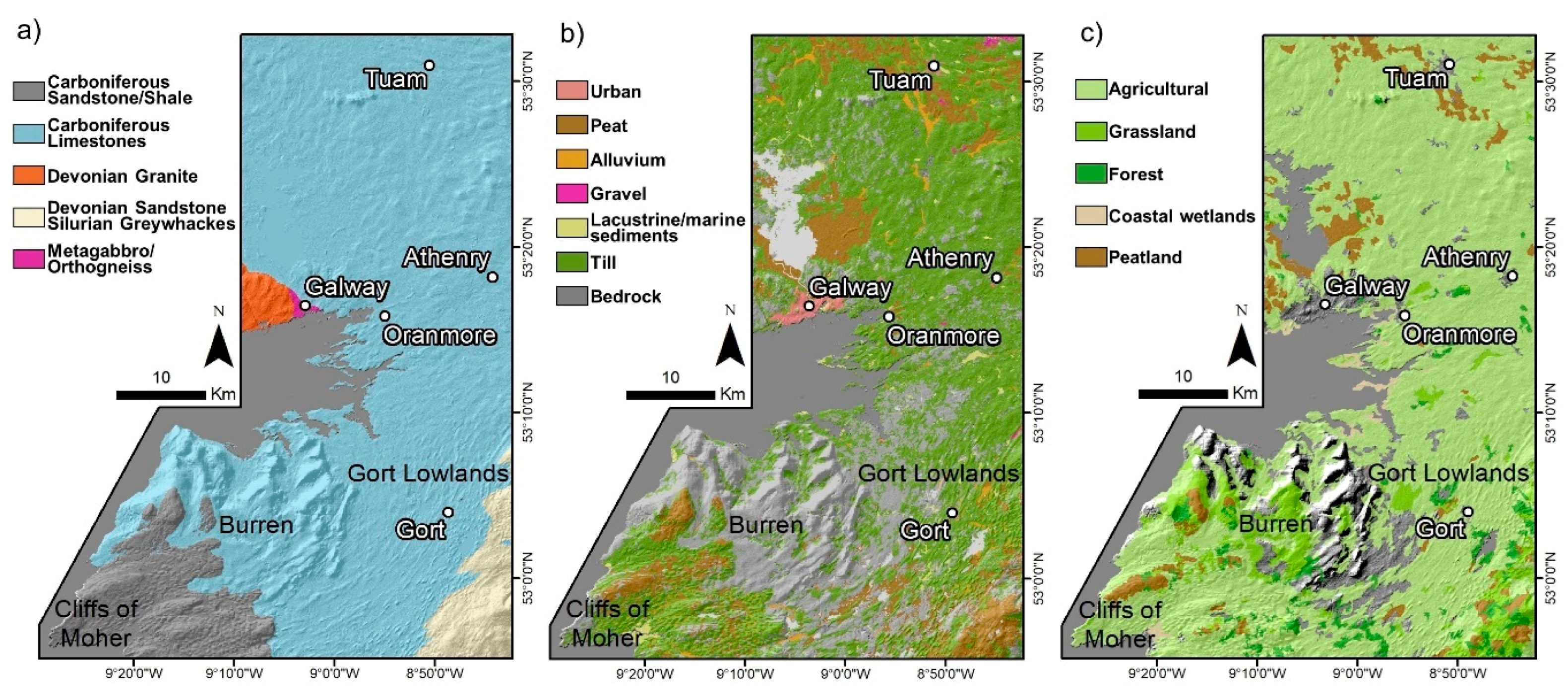
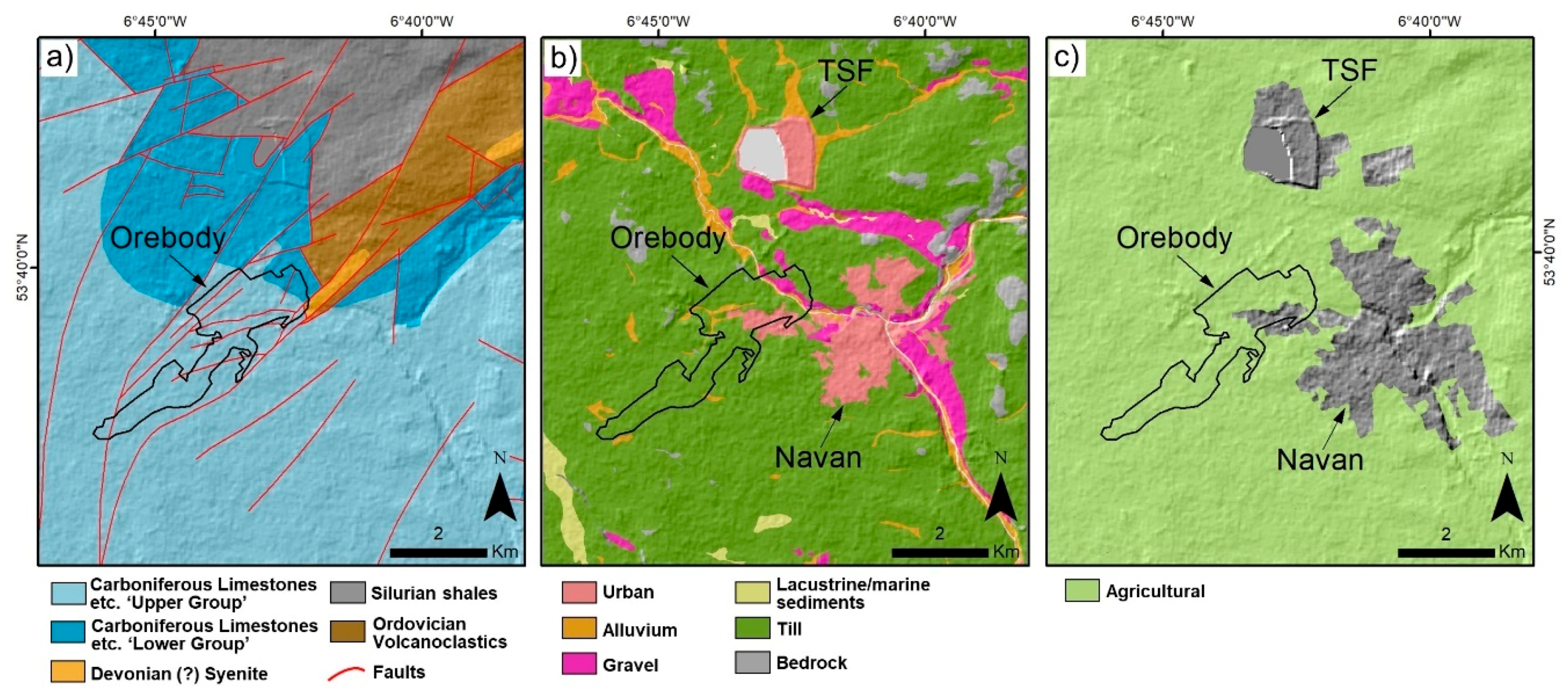
The island of Ireland is affected by numerous small-scale ground instabilities related to either land-sliding, peatlands, karstification, fluvial or coastal erosion (Figure 2) [22,23,24]. Other instabilities relate to past or current anthropogenic activities, mainly drainage, construction, and mining. Whether natural, manmade, or a combination of both, all such instabilities can have serious local consequences in terms of damage to buildings and infrastructure, interruption of services, economic losses and potential for environmental and cultural losses.

Landslides in Ireland can occur in rock, “mineral” soils, or organic soils (i.e., peat), and they are most common in upland areas and coastal areas. Landslides in rock comprise falls, topples or rotational/translational slides controlled by chemical/physical weathering or rock mass discontinuities (bedding planes, joints and faults). In the Irish context, instability of “mineral” soils, which are predominately glacial tills [25], may result from pore water pressure and/or internal erosion within steep slopes cut through these soils.

Peat-related instabilities occur as a consequence of natural processes (heavy rainfalls, alternation of dry and wet periods) or in combination with anthropic activities (e.g., turf cutting, land drainage, construction activities). In addition to being sources of landslides, peatlands in Ireland have long been causes of geotechnical hazards as a result of the low shear strength and high compressibility of peat [26]. Irish peatlands comprise three distinct landscape units: raised bogs, blanket bogs and fens [27,28]. A recently-introduced fourth category, cut-over peatland, describes peat areas harvested for industrial purposes. Raised bogs are groundwater-fed and located mainly in the Irish midlands. Their depths average 6–7 m, but may reach 14 m [29]. Vegetation is dominated by moss (Sphagnum), with minor heather, bog cotton, and others also present [30]. Blanket bogs are rainfall-fed and are mainly confined to the west coast of Ireland and to mountainous areas [31]. They form a blanket-like layer varying in depth from 1 m to 6 m [32]. Vegetation is dominated typically by bog cotton (Eriophorum), as well as black bog rush, and purple moor-grass [30]. Fen peats usually occur at the base of raised bogs and they typically grow in river floodplains or in interdrumlin flats [33]. Fen peats may potentially underlie adjacent urban development that could lead to ground instability.

Ground instability related to karst is a potentially widespread hazard in Ireland. Carboniferous limestone is the outcrop or subcrop of over 50% of the Republic of Ireland [34], and its extensive karstification is indicated by karst drainage and landforms in 80–85% of the limestone outcrop area. Typical of karst terrains are underground fissures and cavities dissolved out of the bedrock by acidic groundwater. Collapse of overlying rock and/or soil into these features can result in sinkholes. These are depressions that range in diameter from 1 m to 500 m and may form over tens of years or tens of minutes [35]. Karst terrains therefore present special hazards to the construction and long-term stability of roads, railways, and buildings (e.g., [36]).

Ireland has 3171 km of shoreline [37], much of which is cliffed coast that undergoes erosion related to both direct wave attack and the effects of swash run-up to cliff base [38,39]. Rock-dominated coasts are present mainly in the southwestern, western, and northern regions of Ireland, while the eastern and south-eastern regions are made of unconsolidated Quaternary sediments [40]. The coasts, particularly those of western regions, are exposed to the full effects of eastwards-moving cyclonic weather systems and swell wave energy from the north Atlantic (e.g., [41]). The Irish coastline, and prominent cliffs in particular, nonetheless represents an important tourist attraction. For example, the Cliffs of Moher area (Co. Clare), is one of the main natural attractions in Ireland with almost 1.5 Million visitors per year [42].

The detection and monitoring of such geological hazards with traditional ground-based methods, such as levelling, is usually expensive and time consuming. Moreover, instabilities often occur in remote places not easily accessible, leading to information gaps. Traditional remote sensing techniques used to try to fill such gaps have involved analysis of high-resolution optical images from satellite-based or airborne sensors. More recently, these have been complemented by analysis of digital terrain models derived from airborne light detection and ranging (LiDAR) [43]. Such techniques are limited in areas of temperate oceanic climate such as Ireland, however, by cloud coverage that is frequently extensive at low altitude and by attendant precipitation. In addition, these approaches have tended to be very expensive which can be a limiting factor for low budget projects and/or for large-scale studies. Satellite-based radar imaging offers a potential solution to such limitations, as radar can penetrate cloud cover and can operate during day and night under all-weather conditions. In particular, multi-temporal InSAR techniques can potentially measure mm-scale ground motions and, thus, help identify and study geological hazards, particularly in relation to infrastructure and buildings [44]. Rates of some ground motion events in Ireland, such as landslides or sinkhole collapses, could in principle exceed the ones detectable by InSAR due to local image decorrelation. Nonetheless, precursors to such very rapid motions, as well as slower ground motions linked to other causes, may still occur at detectable rates. One other great advantage of multi-temporal InSAR techniques is the ability to look back in time thanks to archive data starting from more than two decades ago that provide important data sets for understanding the process involved in ground displacements.

3. Study Areas

We focus here on two areas of interest (AOI), one in the west and one in the east of Ireland (Figure 3). AOI-1 is a ~1800 km² area spanning north County Clare and east County Galway. This area contains a wide variety of landscapes from urban to rural. The former includes the city of Galway (population ~80,000), while the latter includes grassland, forest, peatland, rock outcrop or combinations of these. AOI-2 is a ~100 km² area covering the Tara mine site in Co. Meath, 40 km northwest of Dublin. The landscape in AOI-2 also varies from urban and rural, with the former represented by the town of Navan (population ~30,000) and the land-cover of the latter characterized mainly by agricultural land.

The geology of both AOIs is dominated by Carboniferous limestones (Figure 4a and Figure 5a). In AOI-1, the underlying limestones are relatively pure, and so karst landforms are especially well developed there. AOI-1 includes the Burren and Cliffs of Moher UNESCO Global Geopark. The Burren is an area of spectacular upland karst characterized by expanses of bare limestone rock and minimal surface drainage. Much of the rest of AOI-1 is mantled lowland karst, which includes the ecologically sensitive Gort Lowlands [45]. AOI-1 also has bedrock composed of (1) Devonian granite west of Galway city, (2) Devonian mudstone, siltstone and conglomerate south east of Gort and (3) Carboniferous shale and sandstone sequences around the Cliffs of Moher. Pleistocene and Holocene superficial deposits overlying the bedrock mainly comprise glacial till, as well as lacustrine deposits, alluvial sands and gravels, and peat. The bedrock of AOI-2 (Figure 5a) is mainly composed of (1) Carboniferous muddy limestones (2) Devonian syenite intrusions (3) Silurian mudstones, siltstones and greywacke and (4) Ordovician tuffs, muds, silt, and volcanics. The Tara mine in AOI-2 is the largest operational lead-zinc mine in Europe. The mining activity follows mineralization in a ‘lower group’ of Carboniferous limestones, which occur at depths increasing from 50 m below sea level (b.s.l.) to 1900 m b.s.l. towards the southwest. Solid waste arising from metal extraction is gathered in a Tailing Storage Facility (TSF) located 2 km north of the mining area (Figure 5b).

4. Data and Methods

The data comprise SAR images acquired in C-band (5.6 cm wavelength) and vertical co-polarization (VV) by the Sentinel-1A/B twin satellites in Interferometric Wide Swath (IW) mode. Each image can cover an area of around 250 km × 200 km, with a ground resolution of ~4 m × 14 m in range (perpendicular to orbit) and azimuth (parallel to orbit) directions, respectively. Each satellite has a revisit time of 12 days, and an effective repeat cycle of six days is possible by combining both satellites. For the AOI-1, we used 124 images (track 96, descending orbit) covering the period 4 May 2015–1 March 2018. For AOI-2, we used 117 images (track 125, descending orbit) acquired from 6 May 2015 to 26 January 2018.

The interferometric processing of the SAR images was carried out with the PS-InSAR approach as implemented in the SARscape software package. The principle of the PS approach is to identify point targets represented as individual image pixels, named Permanent Scatterers (PSs), that maintain high radar signal reflectivity over time. This approach relies on a stack of multi-temporal SAR acquisitions to improve the accuracy of displacement measurements and to reduce errors related to transient atmospheric effects. For each point, a displacement time series and a mean velocity rate are calculated.

In detail, the PS interferometric processing chain adopted in this work is based on that of [1,49] and consists of the following steps:

• Image importation: the Single Look Complex (SLC) images comprising radar amplitude and phase information in vertical co-polarization (VV) are imported; the corrections related to the satellites position are made by using precise orbit files (Precise Orbit State Vectors for ENVISAT and Precise Orbit Ephemerides for Sentinel-1, both provided by the European Space Agency (ESA).
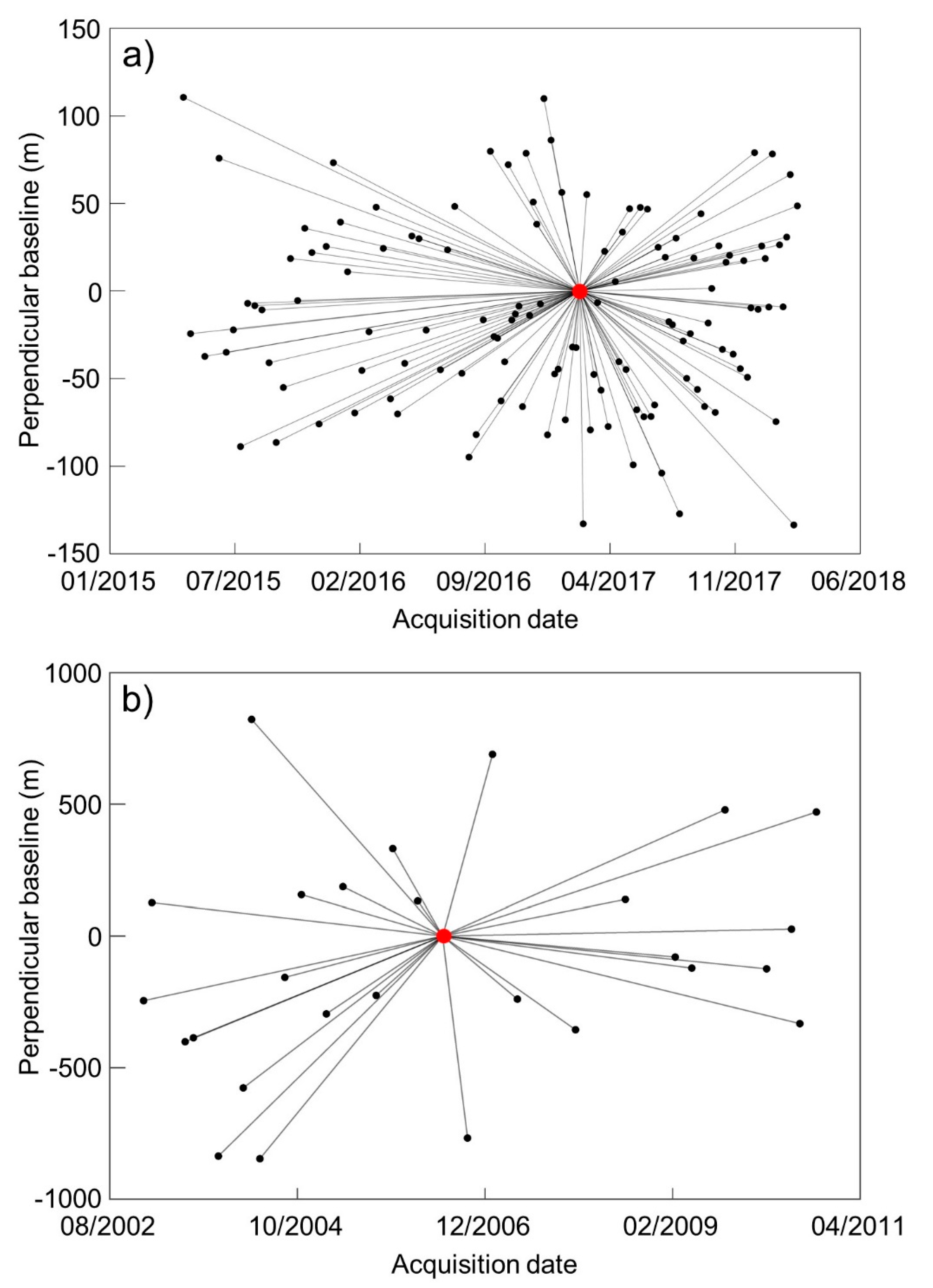
• Connection graph generation: all the images are connected to a master image (selected to minimize the spatial and temporal baselines across the dataset) (Figure 6) in order to obtain the pairs that will be analyzed in the next steps.
• Interferometric processing: the images are co-registered to the geometry of the master image; the interferograms are then generated by pixel-wise subtraction of the phase information in each image. The phase difference due to the topography is removed by using the Shuttle Radar Topographic Mission (SRTM) Digital Elevation Model (DEM) (1 arc second, ~30 m × 30 m resolution) [50]. The remaining phase difference predominantly relates to ground displacement and atmospheric effects.
• PSs identification: the point target candidates are identified by considering the Amplitude Dispersion Index (ADI), which is defined as the ratio between the standard deviation and the mean of the amplitude values of a pixel [1]. Pixels with low ADI in all acquisitions are selected as PSs.
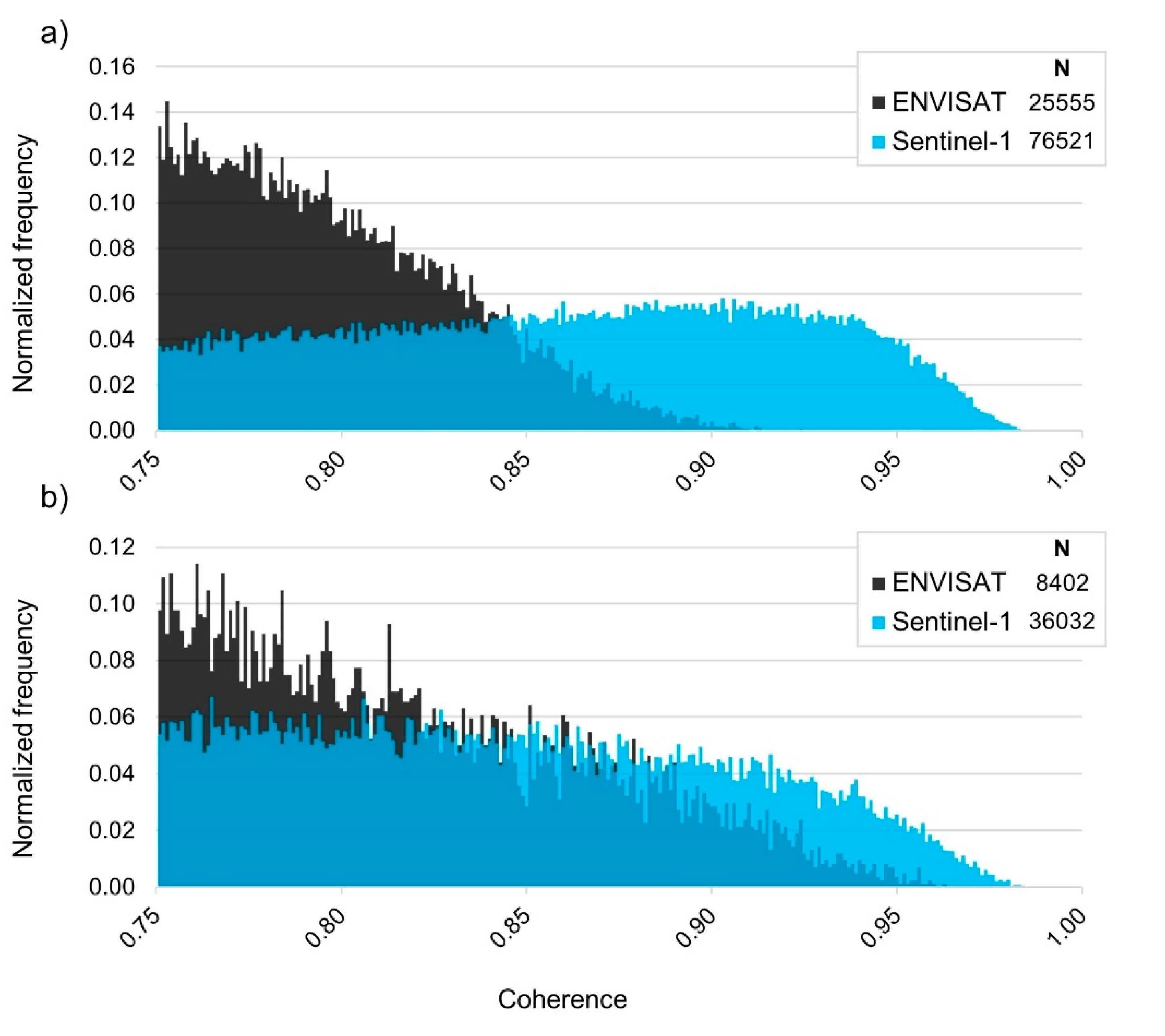
• First inversion: in this step, the phase components related to the topographic residuals and to the displacement velocity are calculated by using a linear velocity model and are then removed from the interferograms. The coherence (i.e., the measure of decorrelation due to temporal and geometric degradation [51]) and elevation of the image pixels are also calculated.
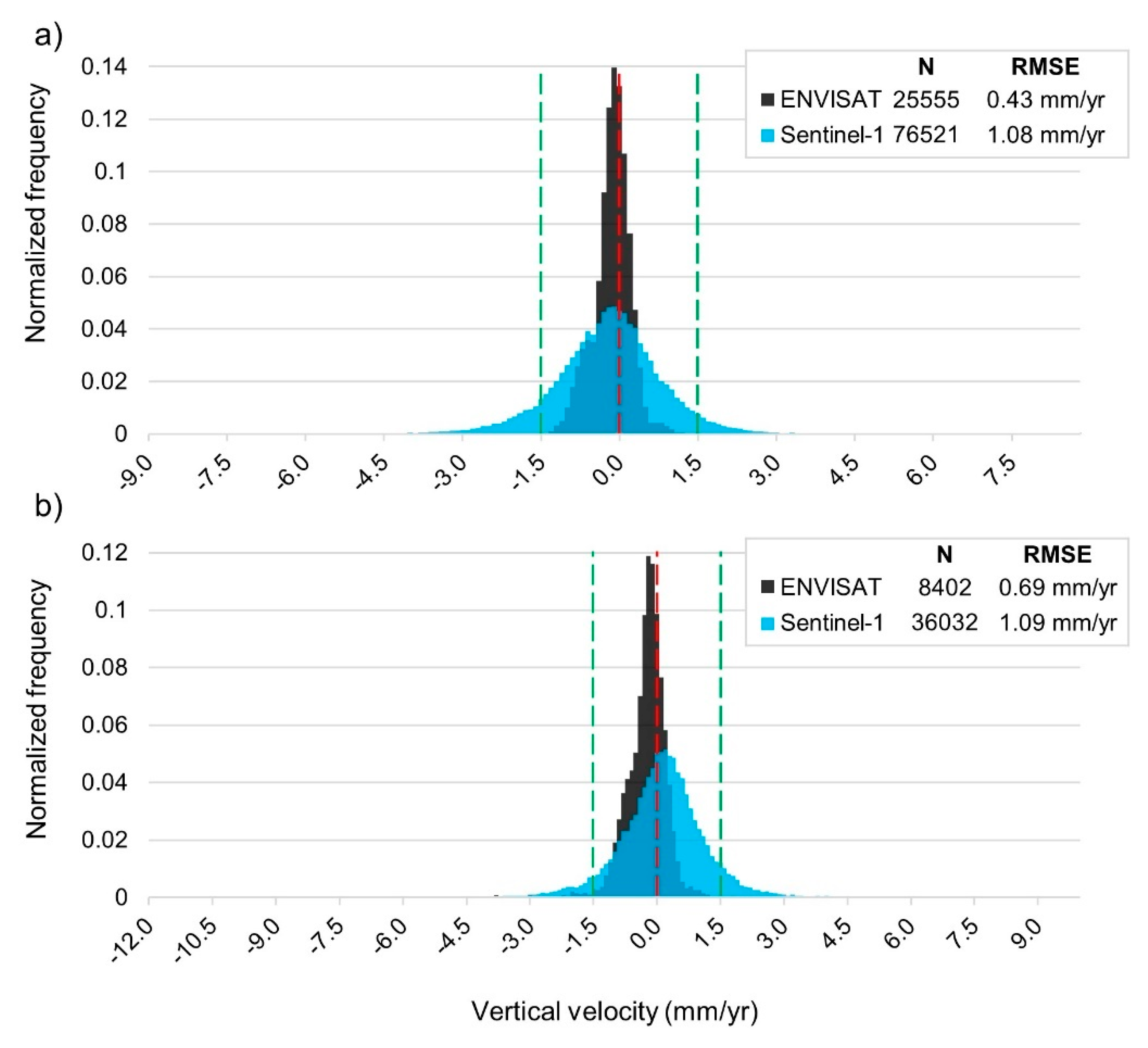
• Second inversion: the atmospheric phase components are estimated using the products of the linear model calculated in the previous step and are subtracted from the interferograms by using high-pass (365 days) and low-pass (1200 m) filters. The PSs with coherence values lower than 0.75 are discarded. Considering such parameters, the precision of the measured velocities was calculated to be in the 0.06–0.39 mm/year range. The precision is calculated with the following formula (after [52]):

  $$\sigma =\frac{\lambda }{4\pi } \sqrt{\frac{1-{\gamma }^2}{2{\gamma }^2}}$$

  in which σ is the calculated precision, λ is the signal wavelength, and γ is the average pixel coherence. Velocities shown in time-series plots below are reported to one significant digit, which thus represents a conservative estimate of the velocity precision.
• Geocoding: the final interferometric products are geocoded into the WGS 84 UTM zone 29N projected coordinate system and exported as shape or raster files for the post-processing analyses.

Given its size and the data volume, AOI-1 was divided in sub-areas of around 10 km × 10 km, each of which was processed independently. A ~10% overlap of these sub-areas was maintained to check the quality and consistency of the results. This approach facilitated a more refined InSAR processing and produced more manageable results for the post-processing analyses.

The SAR images are acquired from an inclined view geometry, with a Line of Sight (LOS) angle of ~33° (θ) from vertical in the case of Sentinel-1 and with incidence angles at the topographic surface ranging from 32° to 35°. Each displacement measurement therefore includes both vertical (up-down) and horizontal (east-west) components. To extract the up–down and east-west components, it is necessary to combine the information provided by both the ascending and descending orbits [53]. The displacement component along the north–south direction cannot be properly measured because the SAR satellites have near-polar orbits and are not sensitive to movements parallel to them. Two further sets of images acquired in ascending orbit (AOI-1: 88 images, track 74, 20 April 2015–05 March 2018; AOI-2: 121 images, track 103, 22 April 2015–24 January 2018) were therefore also processed to assess if an observed movement was dominantly horizontal or vertical.

Two stacks of descending ENVISAT images were also processed over both AOIs, 28 images (track 352) acquired from 07 February 2003–08 October 2010 for AOI-1, and 37 images (track 37) from 07 November 2002–08 July 2010 for AOI-2. Both image sets have VV polarization, LOS of ~23°, revisit time of 35 days and ground resolution of ~20 m × 4 m, respectively, in range and azimuth directions. The obtained results are used for comparison with those of Sentinel-1 in terms of number of detected points, point density and noise level. Lists of all Sentinel-1 and ENVISAT images used in this study are available in the Supplementary Materials.

Several ancillary data sets were used to contextualize and interpret the interferometric results in a geographic information system (GIS) environment. These included open access data from the Geological Survey Ireland (GSI) [54], on bedrock geology, superficial Quaternary sediments, karst features, fault traces, geotechnical boreholes and land use. CORINE 2012 land-cover data provided by the Environmental Protection Agency (EPA) [55] were used to produce the vegetation land-cover maps of both AOIs. We used infrastructure data provided by Transport Infrastructure Ireland (TII) [56] with a buffer distance of 10 m to define PSs corresponding to the motorway and railway networks in AOI-1. The buffer size was chosen to take into account uncertainties in correspondence of PSs with those linear features, while also excluding as much as possible PSs belonging to adjacent buildings and other reflectors (cf. [57]). For all localities of detected motion, 0.25 m resolution aerial imagery acquired by BlueSky International in May 2017 were used to provide visual context to the obtained PSs.

Finally, field surveys were carried out in June and July of 2018 at representative sites of InSAR-defined ground movements. The surveys consisted of visual inspection of the areas to document the nature of the surface features that provide the backscattering signal, to record any damage to buildings or infrastructure (e.g., cracks and fissures) and to check for signs of ground deformation (e.g., uneven surfaces, bulging or depressions of road pavement, etc.).

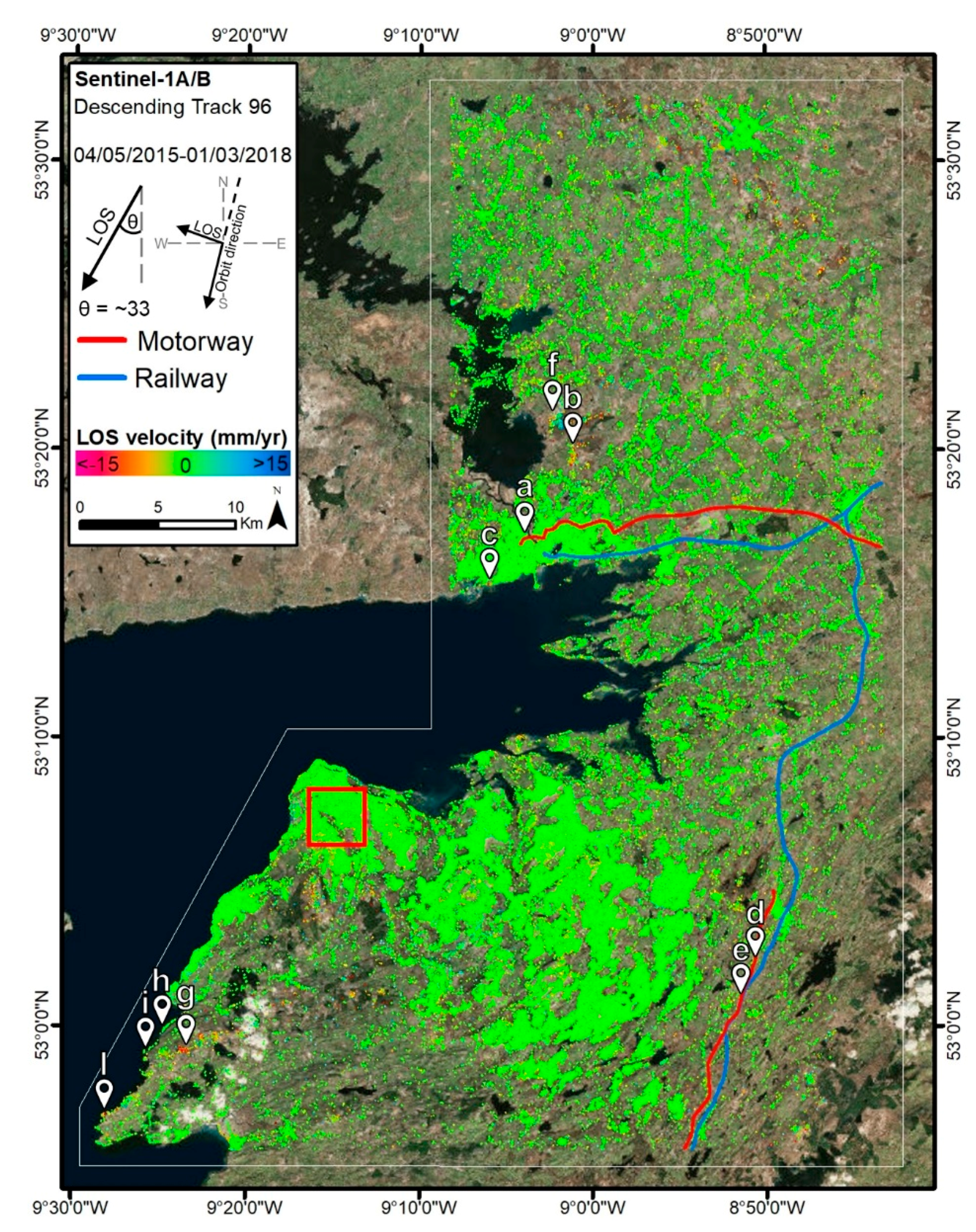
5. Results for AOI-1

Over 1.49 million PSs were defined from the processing of the Sentinel-1A/B images for AOI-1 (Figure 7). The velocities along the satellite LOS at these points are classified as follows: negative values are the points moving away from the satellite (yellow to purple) typically indicating ground subsidence; positive values are the points moving towards the satellite (cyan to blue) typically indicating ground uplift; points considered as stable have velocities in the range of ±1.5 mm/year (in green), which corresponds to the accuracy obtained by past ground validation of C-band satellites such as ERS-1/2 and ENVISAT [58].

The distribution of PSs strongly depends on the reflectivity and coherence characteristics of objects on the ground. The highest point densities are obtained in the Burren area (density of 3407 points/km²), where limestones outcrop with very limited or totally absent vegetation cover. High point densities were also obtained in Galway city (density of 2545 points/km²) and in the towns of Oranmore, Tuam, Athenry, and Gort. Although the average point density obtained over the vegetated lowlands (density of 302 points/km²) is more than ten times lower, and in many parts points are lacking entirely, the regional road network in these areas can be recognized, probably as consequence of back-scattering from buildings along these roads. The monitored territory appears to be generally stable. No large-scale areas (>10 km²) of movement have been detected.

In contrast, only 499,478 PSs are obtained from applying the same processing to the ENVISAT dataset (Figure 8)—about one third of the number obtained from the Sentinel-1 imagery. Most of the points are again located in the outcrop-dominated areas of the Burren, but the density here is 1331 points/km². Although also sparser, the PSs distribution again defines well the urban areas of Galway city, Tuam and Athenry. The rural road networks are not visible in the ENVISAT results, however, as consequence of the far lower PSs density of only 57 points/km² obtained for the lowlands.

In detail, the velocity map derived from Sentinel-1 imagery (Figure 7), however, shows several small-scale (<1 to 6 km²) areas of movement. We categorize these into instabilities affecting anthropic or natural environments. The first category generally comprises local subsidence affecting areas of recent urban development, the road/railway network and the embankments along the coastal areas. The second can be recognized as landslides or unstable slopes occurring along the coastline and as subsidence or uplift (or both) occurring in peatlands. There is no direct evidence of ground movements related to the development of karst features, even if some of the detected instabilities could be explained by active karst processes.

5.1. Anthropic Instabilities in AOI-1

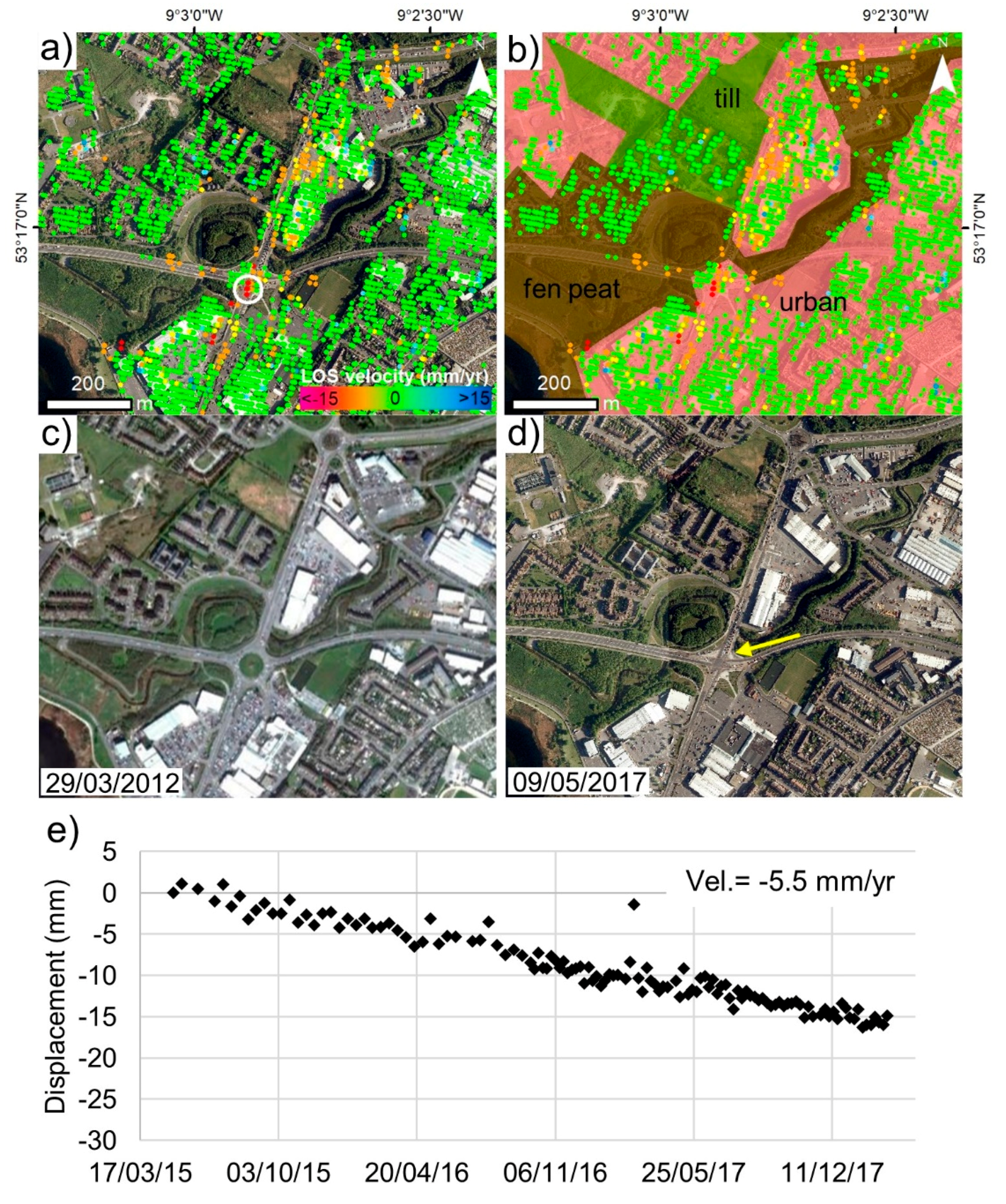
5.1.1. Urban Areas

Only ~1% (19 km²) of AOI-1 is classified as urban, for which 82,789 PSs have been measured. Galway city (15 km²) represents 79% of the urban area and yielded 66,714 PSs. Only 5677 urban PSs are unstable (outside the ±1.5 mm/year range), and most of these are located in Galway city. Here the unstable points are unevenly distributed in small clusters over the paved roads and in proximity to large buildings.

An example of the clustered distribution of unstable PSs in Galway city, marked as ‘a’ in Figure 7, is seen in an area around the intersection of the N6 and N84 roads (Figure 9a). Urban development has here taken place on areas of largely fen peat (Figure 9b). Field reconnaissance revealed that the subsidence areas north and south of the road intersection correspond mostly to car parks (parking lots) that present uneven surfaces and several patches of recently repaired asphalt. The ground surface south of the intersection shows damaged surfaces and tilted light poles. The N6 and N84 roads themselves also show a few depressed and bumpy areas corresponding to the detected subsiding PSs. The highest subsidence rate of −8.4 mm/year occurs at the N6/N84 intersection, the nature of which was changed from a roundabout to a signal-controlled junction at some time between 2012 and 2017 (Figure 9c,d).

A similar pattern is observed in a semi-urbanized area marked as locality ‘b’ in Figure 7 and located north of Galway city along the N84 (Figure 10a). Here, the local subsidence zones correspond to recent land-use changes made to an area of cut-over raised peat (Figure 10b) between 2006 and 2011 (Figure 10c,d). These land-use changes include excavations, some extensions to industrial buildings and the construction of two ‘halting sites’ for mobile homes of the Traveller community (an itinerant ethnic group of persons native to Ireland). Field reconnaissance revealed some possible structural manifestations of ground movement, such as cracked or tilted walls and very uneven asphalt road surfaces, especially in the halting sites, which are apparently subsiding at rates of up to −14.4 mm/year.

Potential ground movements in Galway city were found also at locality ‘c’ in Figure 7, along the coastline (Figure 11). The example here is a 4–5 m high embankment made of metric-scale boulders and reinforced with cement cover (Figure 11a,b). A 200 m long section of this embankment is potentially affected by subsidence up to −6.4 mm/year (Figure 11c). The movements are prevalently vertical, as confirmed by the results obtained with the ascending track. The visual inspection of the area revealed water seepage onto the tidal flat from underneath the subsiding section of the embankment. The seeping water possibly flows from a small stream and several ponds in an adjacent marsh and golf course located behind and upslope of the embankment. Fresh cracks in a few fixed boulders in the embankment were also visible during field reconnaissance.

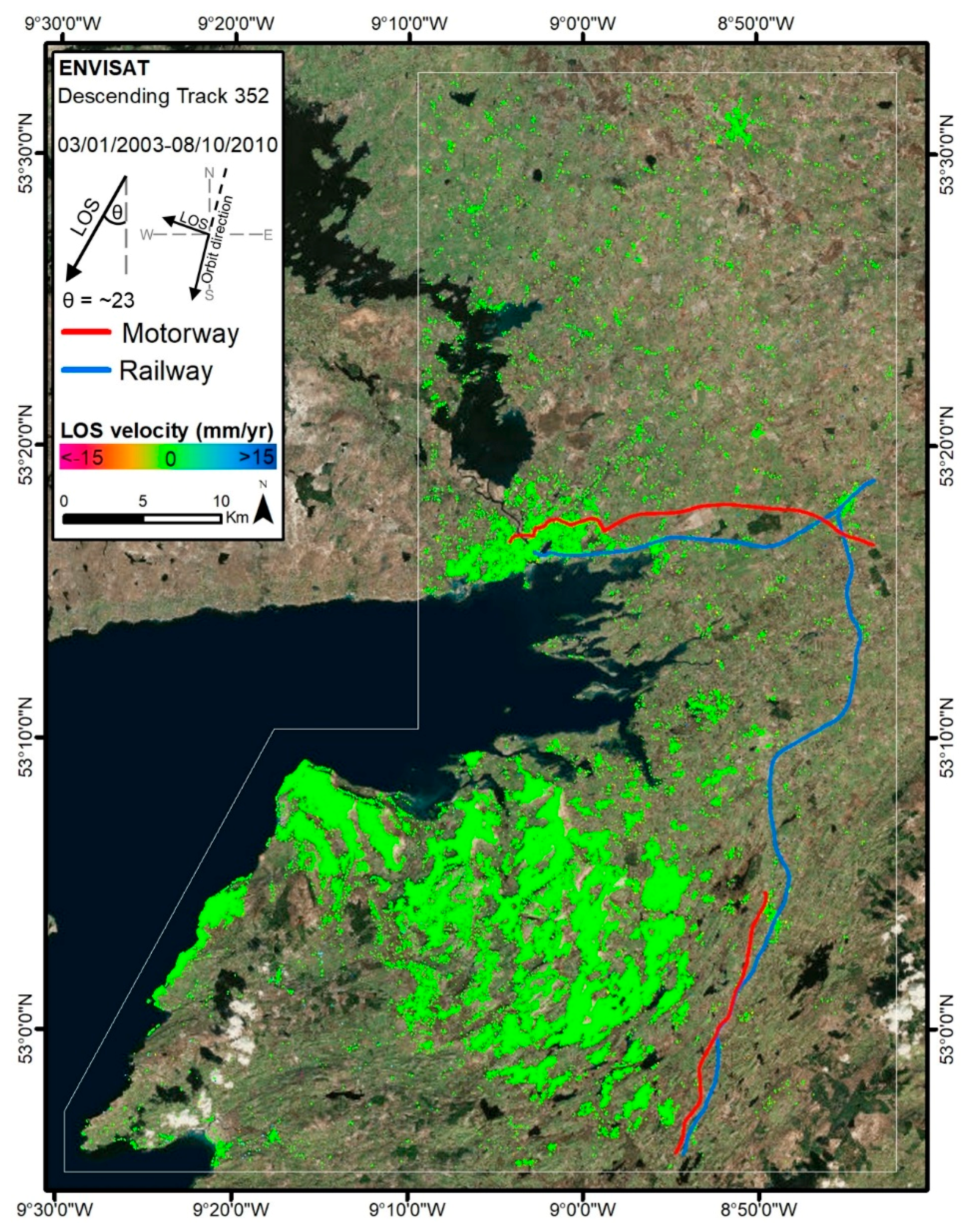
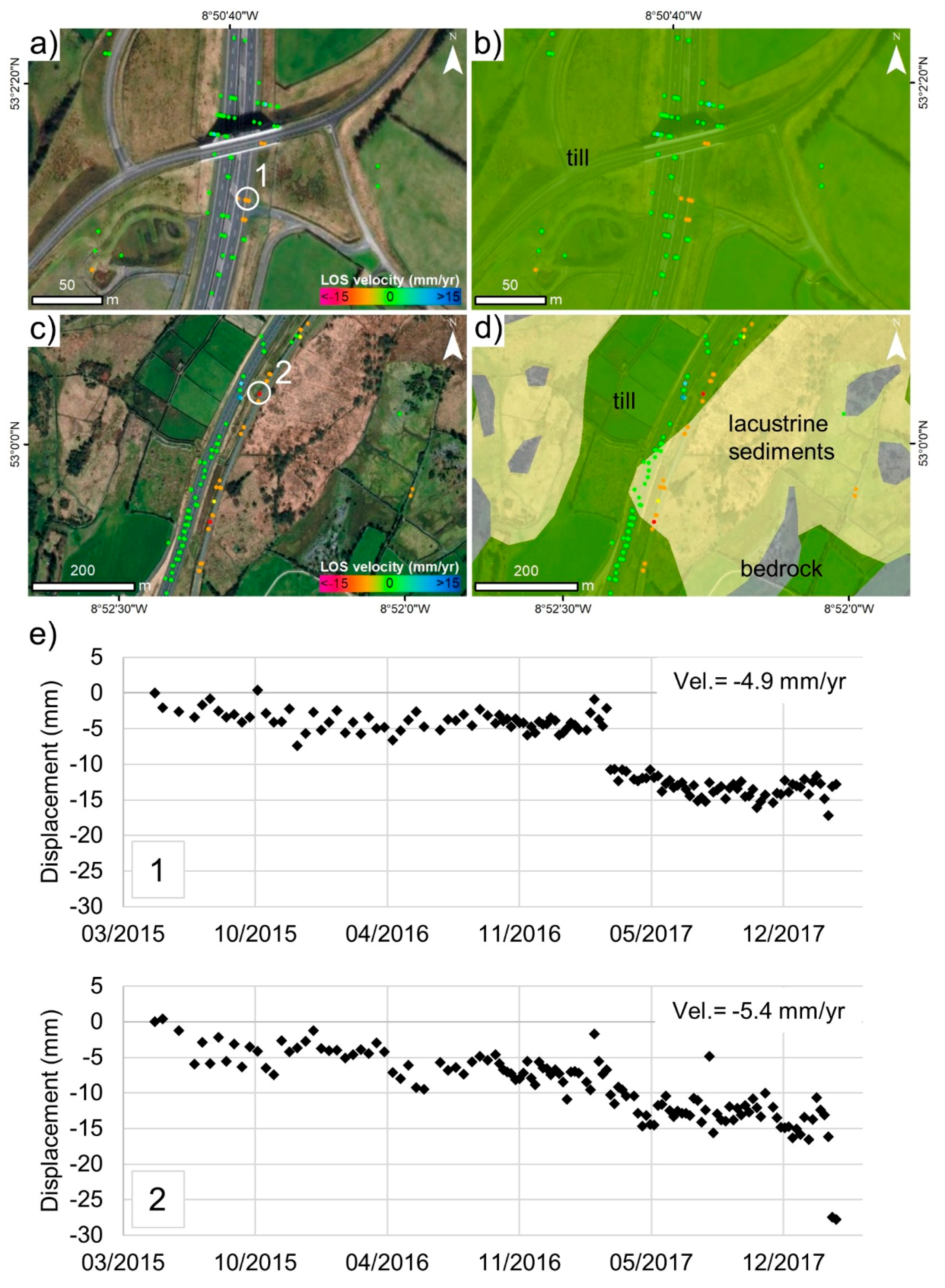
5.1.2. Motorway and Railway Infrastructure

In this study, we analyzed in detail an 18 km-long section of the M18 motorway running north-south near the town of Gort, and a 25.6 km-long section of the M6 and N6 roads running east–west from Athenry to Galway (Figure 4 and Figure 7). The M17 motorway section connecting Gort to Tuam, which opened in September 2017, was not detected by the PS-InSAR analysis due to its very recent construction. A total of 2,779 PSs were extracted over the roads with the 10 m buffer, among which only 253 were outside the ±1.5 mm/year range and hence considered unstable. Most of these points are in Galway city in the area already shown in Figure 9. Other subsiding points with velocities of up to −4.9 mm/year and marked as locality ‘d’ in Figure 7 were detected over one localized section of the M18 motorway (Figure 12a). The field reconnaissance revealed several slightly depressed, uneven and recently re-surfaced areas of the motorway in correspondence with several of the detected subsidence signals.

AOI-1 contains 72 km of the Irish national railway system. The Galway–Limerick route runs north-south for 48 km; the Dublin-Galway route runs east–west for 24 km. Using the 10 m buffer, we extracted a total of 2913 PSs along these railway sections, 701 of which are regarded as unstable. A maximum velocity of −16.4 mm/year has been detected on the Galway–Limerick line at the 38th km mark, while a maximum velocity of −8 mm/year was detected for the Dublin-Galway line at the 23.5th km mark. The respective maximum cumulative displacements produced in the 2.8 years period covered by this analysis are −46 mm and −20 mm. One example of unstable area, marked as locality ‘e’ in Figure 7, is presented in Figure 12c. The railway appears to be built on an embankment immediately over the ground at the base of a slope. The nearby motorway, which runs parallel to the railway for around 3 km, is located up slope. Boggy and marshy areas with high vegetation (reeds) are present close this location.

5.2. Natural Instabilities in AOI-1

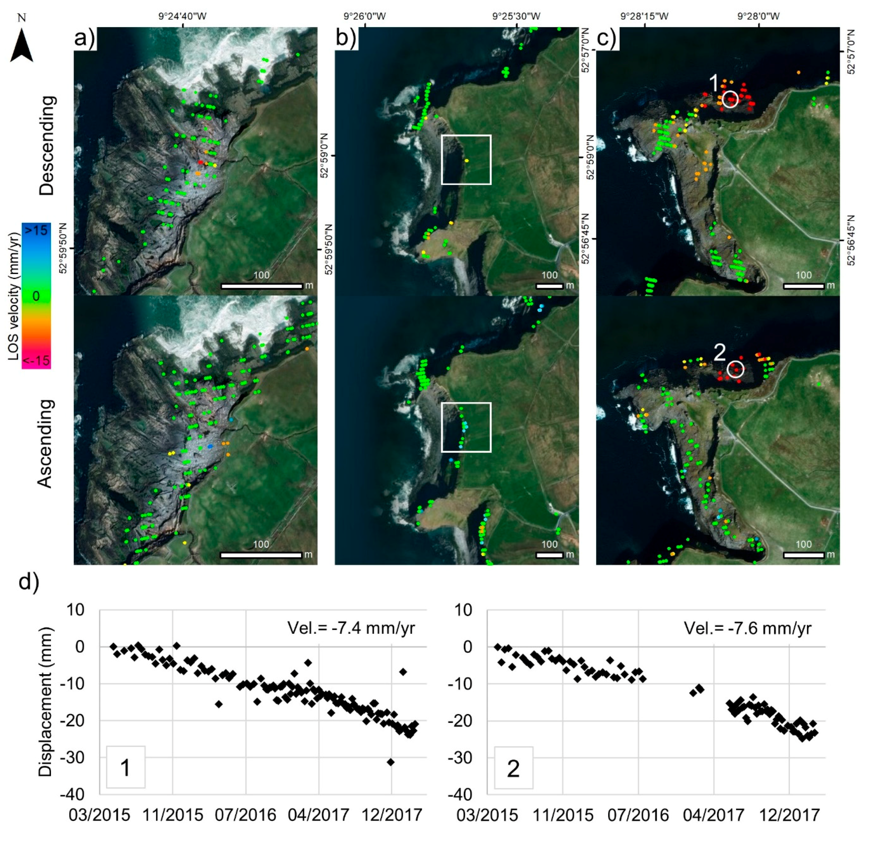
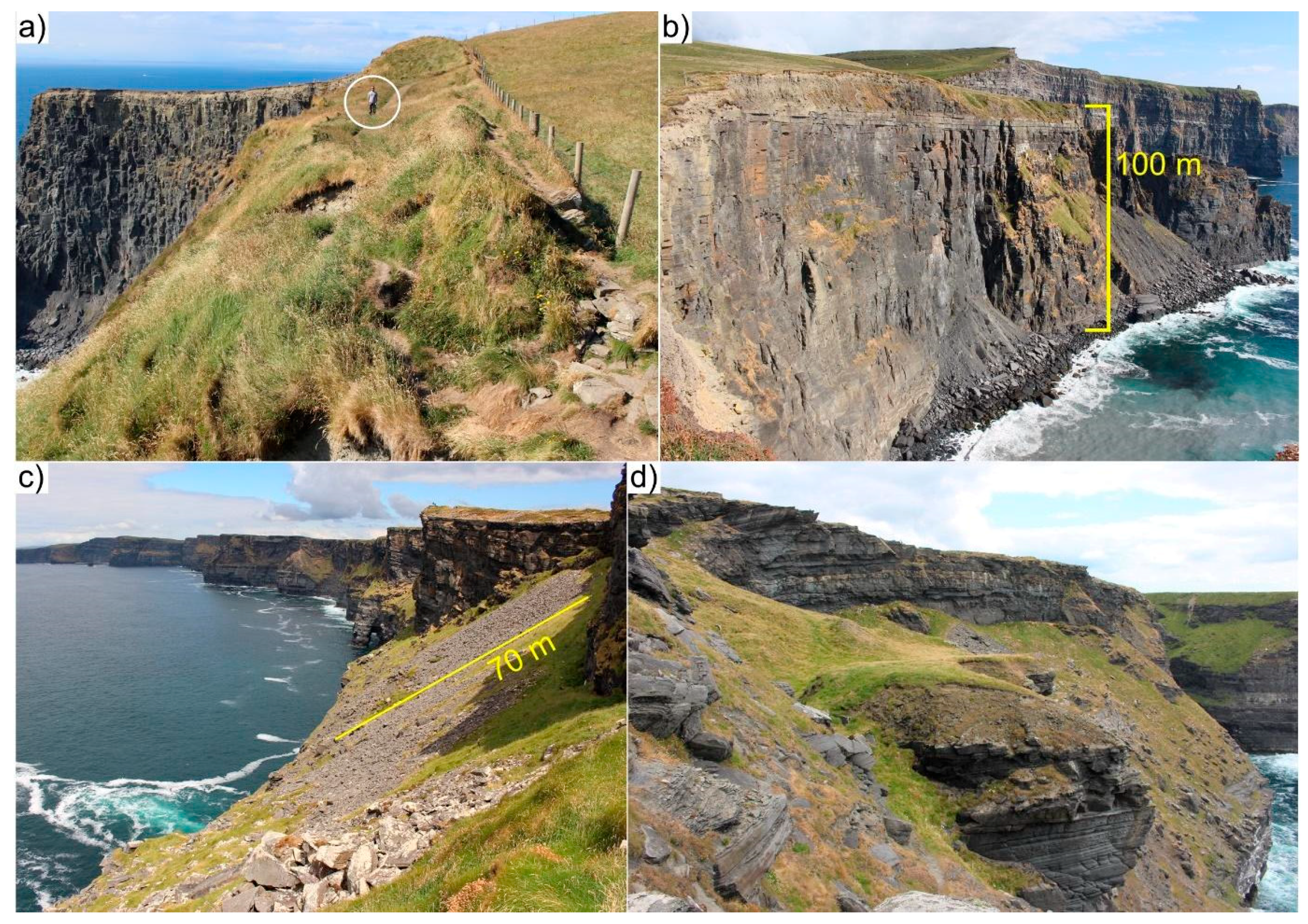
5.2.1. Landslides/Slope Instabilities

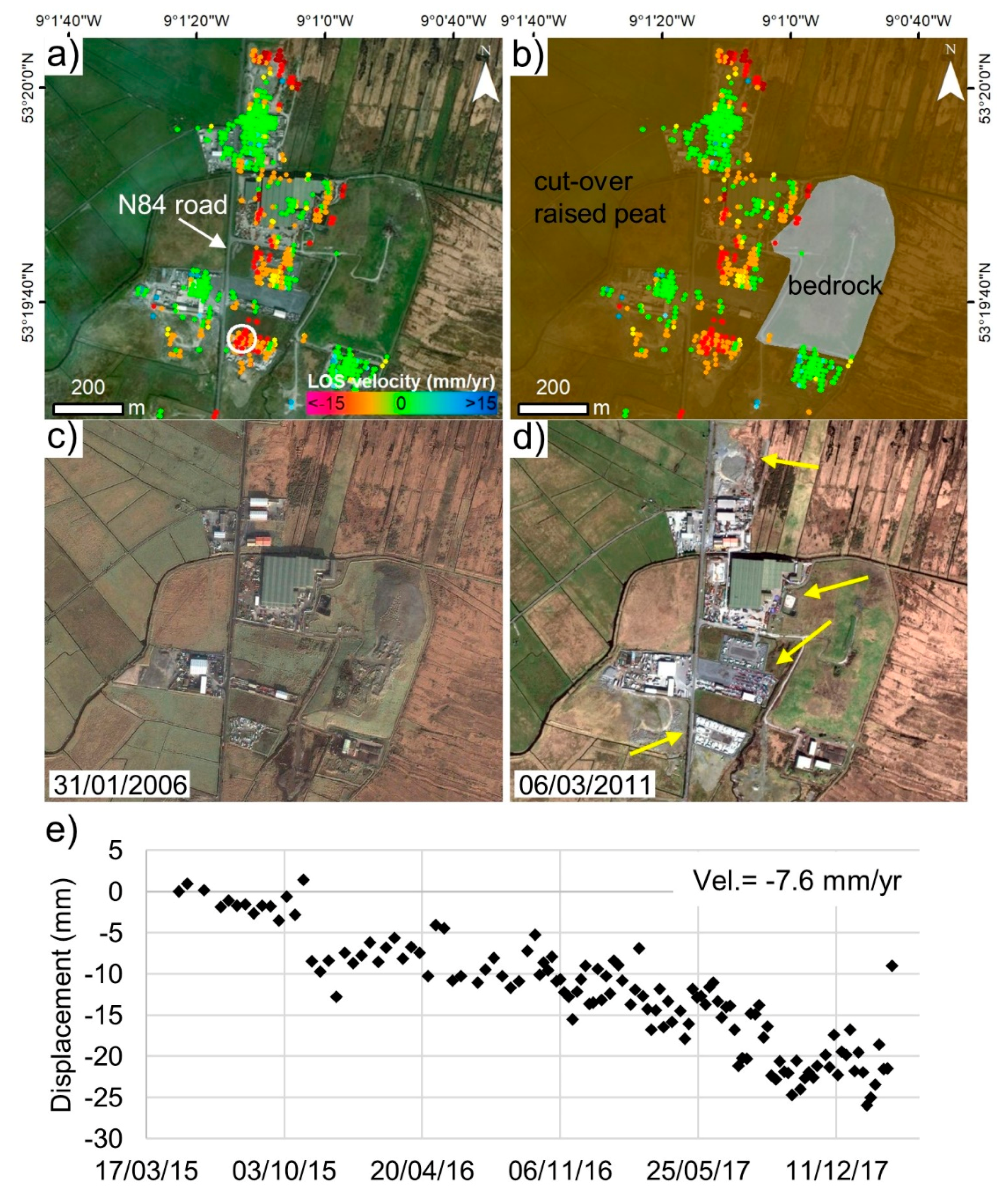
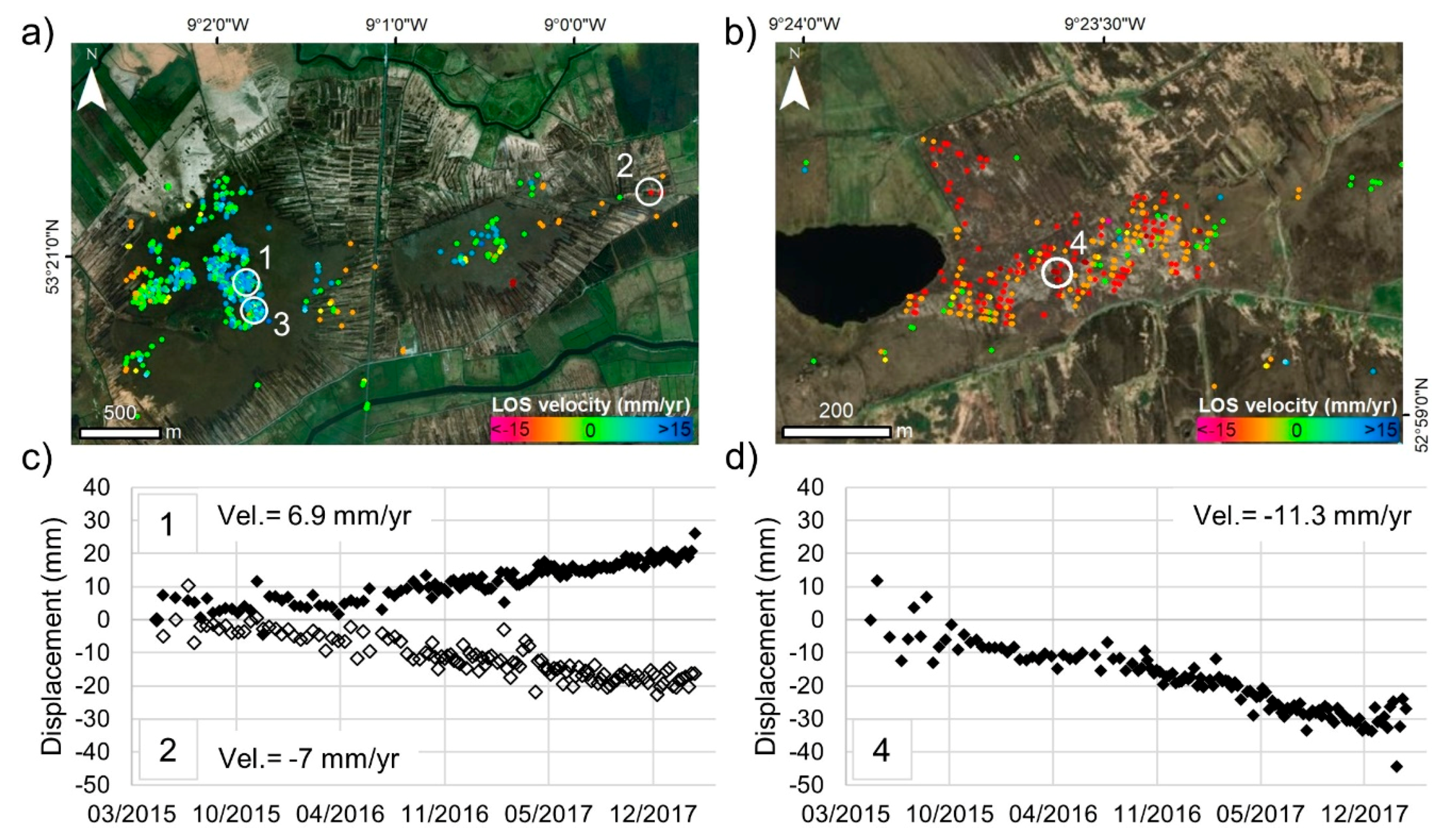
Several small-scale coastal instabilities have been detected in AOI-1 (Figure 13). All occur at or near to the Cliffs of Moher in Co. Clare, and they are marked as localities ‘h’, ’i’, and ‘l’ in Figure 7. The maximum LOS velocities measured at each locality with the descending track are −5.1 mm/year, −2.8 mm/year and −16.9 mm/year, respectively. The maximum values obtained with the ascending track are respectively 6.4 mm/year, 2.6 mm/year and −8.9 mm/year. The movements at localities ‘h’ and ‘i’ have strong horizontal components, as confirmed by the analysis of the ascending track, which presents PSs with opposite velocity signs (Figure 13a). The main area of motion in locality ‘l’, located on the north side of the Hag’s Head (Figure 13c), shows almost identical negative velocities in ascending and descending viewing geometries. The movements are mainly vertical, although, given the north-facing slope, a horizontal component of motion (not detectable by the satellites) cannot be precluded.

Field reconnaissance of localities ‘i’ and ‘l’ revealed many features compatible with ground instability (Figure 14). At locality ‘i’, which occurs at a pronounced embayment in the cliff line, the cliff top comprises a veneer of glacial till overlying the Carboniferous rocks. Old walking paths along the cliff edge are now truncated by the cliffs, and the field boundary wall is locally tilted seaward (Figure 14a). Furthermore, the cliff face is relatively fresh looking (not lichen covered) and there is a fresh (active) talus/debris fan at the cliff base (Figure 14b). At locality ‘l’, the PSs correspond mainly to talus fields on the upper flanks of the Hag’s Head promontory (Figure 14c). Immediately up slope of both talus fields are sharp scarps. The Carboniferous bedrock around Hag’s Head shows marked local rotations and several fissures or cracks are observable between bedrock blocks (Figure 14d). Field reconnaissance and imagery from the Irish Coast Guard [59] further show that the cliffs here are undercut by a pronounced wave-cut notch and several sea caves.

5.2.2. Peatlands

Surface movements in different peatlands in AOI-1 have been detected through the PS-InSAR approach. The best example, marked as locality ‘f’ in Figure 7, is a 6 km² area of cut-over raised peat located north of Galway city (Figure 15a). Some 939 PSs, of which 606 are unstable, are distributed unevenly in the peat area. The majority occur in the central, intact part of the peat ecosystem, while only a few points are located along the harvested margins. Moreover, the central part of the peatland is generally moving upward at rates of up to 8.9 mm/year (e.g., point 1), while the marginal harvested areas are subsiding by up to −11.6 mm/year (e.g., point 2). A transition between the two areas represented by stable points can also be observed.

While some points (e.g., at locations (1) and (2)) have linear long-term displacement trends, others (e.g., at location (3)) display fluctuations that correlate with precipitation amount (Figure 16). Wetter periods correspond to uplift, while periods of drought correspond to subsidence. For example, the 38-day interval from 03 April 2017 to 11 May 2017 had an average rainfall of 0.21 mm that corresponds to a total lowering of 6 mm detected in five consecutive dates, from 11 April 2017 to 11 May 2017. During field reconnaissance in July 2018, we noted that the harvested areas were dry with tall, re-growing vegetation. Moving towards the center of the bog, water content increased, and white moss (Sphagnum) started to appear. The water table was around 20–40 cm below the surface near the bog center, as seen in cracks. At the center of the intact bog, was observed a slight change in vegetation given by taller leaved plants.

Surface motions were also detected in a 1 km² area of blanket peatland in west Clare (Figure 15b), marked as locality ‘g’ in Figure 7. Out of 358 PSs, 324 are unstable. No consistent signs of uplift (only five isolated measured points) were found in this case. Instead, this peatland is dominantly subsiding at rates of up to −16 mm/year. Field reconnaissance again revealed that the areas of highest point density corresponded to unharvested areas dominated by Sphagnum mosses, where peat cover over bedrock is thin (a few tens of cm) or even absent. Formerly harvested areas are now overgrown by dense deep vegetation cover (bracken) and yielded few to no PSs.

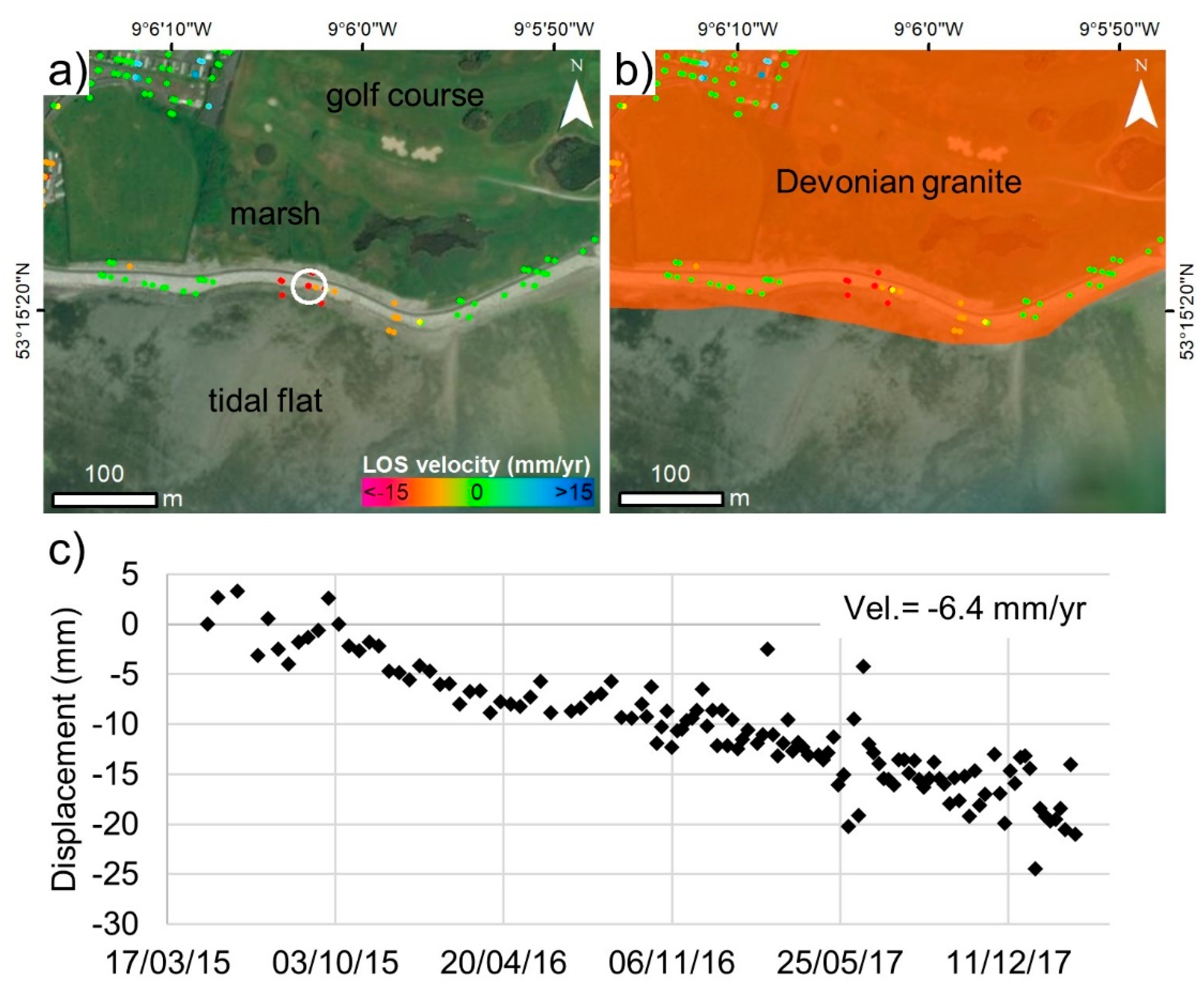
6. Results for AOI-2

A total of 56,568 PSs has been measured in AOI-2 (Figure 17a). Most of the points are distributed over the urban areas, outside of which the data density drastically decreases. Although this reduced the possibility to detect movements over the central section of the mine, it was still possible to make observations in its northern and south-western extents and in the TSF area. Most of AOI-2, including the urban area of Navan, is unaffected by significant land motion (values in the range of ±1.5 mm/year). In comparison to Sentinel-1, the processing of the 2002–2010 ENVISAT images over the same area (Figure 18) provided only 11,740 PSs, which are mainly located over the urban area. In this case, no PSs were obtained over the TSF, either because the embankment surfaces were less reflective at that time (less paved) or because of construction work on the embankment between 2001 and 2005.

Ground motions in AOI-2 were observed only in the area of mining activity and at the TSF. An area of more recent mining activities [46] under several houses, commercial buildings and part of the M3 motorway (Figure 17b) is associated spatially with InSAR-measured land settlement up to -6.8 mm/year that is linear from mid-2015 to early-2018 (Figure 19). No discernable damage to the buildings or the motorway has been observed during a brief field reconnaissance conducted in the area in July 2018. Points showing both subsidence and uplift are present in the main mining site (Figure 17c). Some of the buildings located in the north of this area appear to be affected consistently by subsidence of up to −3.7 mm/year (Figure 19). The highest velocities in AOI-2 occur over the TSF area (Figure 17d), the height of which was increased in 2015. The PS-InSAR results indicate subsidence of up to −17 mm/year (Figure 19) at the top of the TSF’s perimeter embankment, with subsidence rates decreasing to the foot of the embankment where stable points have been measured. Analysis of the ascending track images suggests that motion of the embankment is predominantly vertical and is consistent with compaction.

7. Discussion

7.1. Feasibility of Sentinel-1 PS-InSAR for Ground-Motion Detection in Ireland

Studies of using PS-InSAR and Sentinel-1 imagery for detecting ground instability in temperate oceanic climate zones (e.g., [61]) have so far been rarely documented in peer-reviewed scientific literature. This paper presents a new case study of using PS-InSAR and Sentinel-1 data in such climate zones, and the first in Ireland. Recent Sentinel-1-based InSAR studies in such zones (e.g., [62,63]) have employed an implementation [9] of the Short Baseline Subset (SBAS) methodology [2]. The SBAS technique uses a lower-resolution approach that can help in defining large-scale deformations, but it can consequently lose the capability of detecting small-scale movements. For the same data, the full-resolution approach of PS-InSAR has the main advantage of being able to detect smaller-scale movements. As highlighted by our study with Sentinel-1, this capacity can be critical where the dominant scales of motion are small (down to 100 m² or less), such as in tectonically-quiescent regions like Ireland and elsewhere.

Although previous attempts to apply multi-temporal InSAR to Ireland have been based on PS-InSAR but with ERS-1/2 and ENVISAT data [19,20,21], these studies were restricted to urban areas. Here we highlight that the coverage obtained with Sentinel-1 is many times greater in terms of PS number, density and coverage across different land-cover types than is achievable with ENVISAT (e.g., Figure 7 vs. Figure 8). With respect to Sentinel-1 the more limited results obtained with ENVISAT can be mainly related to four factors: (1) the sparser and more uneven temporal distribution of the ENVISAT images; (2) the longer revisit time (35 days); (3) the slightly lower ground resolution achievable (~20 m by 4 m in range and azimuth, respectively); and (4) the larger orbital tube (i.e., the range of the satellite’s geometrical baselines; in the order of ±1 km for ENVISAT and of ±150 m for Sentinel-1; see Supplementary Materials). The main advantage of Sentinel-1 is, indeed, given by both its higher frequency of image acquisition (reduced temporal decorrelation) and its smaller orbital tube (reduced geometric decorrelation), which result in enhanced coherence of the backscattered radar signal (i.e., radar signal changes at each ground pixel in successive images are minimized). This is shown for our study in Figure 20, where the Sentinel-1 PS coherence is distributed toward higher values, especially in the rocky landscape of the Burren. Moreover, the higher image acquisition frequency of Sentinel-1 permits the detection of short-term displacement variations that could be useful to better understand the factors and mechanisms influencing the occurrence of ground instabilities.

Without independent validation (via, e.g., precise levelling campaigns), some caution should be exercised regarding the accuracy of the values of ground motion presented here. Elsewhere, comparison of ground displacement velocities derived from PS-InSAR on ERS-1/2-ENVISAT and Sentinel-1 imagery with ground displacement velocities measured by precise levelling [58,64] indicates that differences are within 1.5 mm/year and 1.0 mm/year, respectively. An evaluation of the noise levels in two apparently stable sub-areas in AOI-1 and AOI-2 (Figure 21) shows that the Sentinel-1 data are slightly noisier than that of ENVISAT. The frequency distribution of velocities of Sentinel-1within these sub-areas spans a wider range than that of ENVISAT, and the mean squared error (RMSE) is higher, about 1.1 mm/year for Sentinel-1 and 0.4–0.7 mm/year for ENVISAT. While 99.9% of ENVISAT data lie within the ±1.5 mm/year stability threshold, 94% of Sentinel-1 data lie within ±2.0 mm/year. Although not affecting the maps presented here (Figure 7, Figure 8, Figure 17, and Figure 18) to any great degree, the latter value may therefore represent a more conservative threshold for ‘stable’ PSs based on Sentinel-1.

In addition to an appreciation of the PS noise level, confidence in the interpretation of the computed PS velocities here, and in other studies, arises from a combination of three other factors: (1) a high density and spatial consistency of points indicating movement along the LOS direction for one acquisition track, (2) a presence of a potential movement signal in both ascending and descending tracks, and (3) a land surface and/or sub-surface material conducive to motion. Assessment based on factors such as these is thus partly subjective and partly dependent on the scale of observation. In this study, we present high-confidence examples of ground motion. One of these (Figure 13b) exhibits LOS velocities within the ±2.0 mm/year range; in this case our confidence in its validity is based on the detection of similar rates of movements but with opposite signs in both ascending and descending tracks and on the observations of instability at that locality in our visual site inspections. In general for all examples of potential ground motion highlighted in AOI-1, visual site inspections and existing data on subsurface materials provided either direct evidence of past ground motions (e.g., sagged roads or collapsed cliffs) or revealed ground conditions that could be plausibly conducive to ground motion (e.g., water seepage or recent construction over peatland). Nonetheless, future work in the application of PS-InSAR in Ireland should involve ground-truth measurements on the ground motion examples presented here and/or in other areas of the island.

Future work will consist also in the use of alternative radar wavelengths to better monitor the transportation network. The main limitation of Sentinel-1 in detecting such infrastructure is given by the geometrical characteristics of the roads (width) in respect to the maximum ground resolution achievable with the SAR images. For this reason, X-band images (e.g., from TerraSAR-X or COSMO-SkyMed satellites), which have higher spatial resolution than currently-available C-band images may be useful for more detailed monitoring of ground movements affecting infrastructure (e.g., [65]). X-band data also have the advantage of being more sensitive to subtle deformations thanks to the smaller wavelength.

The current results could be improved by better estimating and subtracting the atmospheric noise from the generated displacements. The seasonal changes of the stratified atmosphere, which are correlated with time, are in fact potentially not properly estimated by the conventional high-pass filtering implemented in the standard PS-InSAR algorithm [66]. Thus, future work will also consist of using more sophisticated methods for the estimation of the atmospheric delays and the correction of the InSAR-derived time-series.

Overall, the obtained results demonstrate that Ireland, even if geologically very stable, is still characterized by a dynamic and mutable landscape where gravity-driven or water-related ground movements are common at scales of between 10⁻³–10¹ km² and represent the main geo-hazards of the country. The success here of PS-InSAR with Sentinel-1 data in detecting such ground motions makes the technique a good candidate for upscaling such surveying to an island-wide SAR monitoring, as tested recently for neighboring Great Britain [67].

7.2. InSAR-Detected Ground Motions in Ireland (AOI-1 and AOI-2)

In general, the ground motions detected in AOI-1 can be related to compaction of unconsolidated sediments, particularly peatlands, and to coastal erosion processes. Most of the detected velocities are negative in both LOS geometries, indicating that the motions are dominantly vertical (subsidence), and they range between −1.5 and −14 mm/year. One exception to this general pattern occurs in the peatland north of Galway city, where positive velocities are detected in both LOS geometries indicating uplift of between 1.5 and 8.9 mm/year. Another exception occurs on parts of the Cliffs of Moher, where the opposite sign of the detected velocities indicates a large horizontal component of movement.

A plausible, but unverified, explanation for the ground motions detected in urban areas (Galway city) and along infrastructure in rural areas is the compaction of unconsolidated sediments (peat or lacustrine deposits) due to the load produced by the recent construction of roads and buildings. [19,20] proposed this cause also for some ground motions indicated by PS-InSAR in Cork and Dublin through analysis of ERS-1/2 and ENVISAT data and comparison to historical Ordnance Survey maps. Since some sections of the motorway and the railways in AOI-1 pass over highly karstified limestone regions (e.g., the Gort lowlands), however, a relationship of detected motions to karst or epi-karst processes cannot be excluded. Sub-surface geophysical studies or drilling may be required to further test such hypotheses.

Our study also highlights the suitability of the PS-InSAR technique for monitoring both man-made coastal defense structures and natural coastal landforms in Ireland. The detected instabilities on the Cliffs of Moher are not currently registered in the national landslide database [68], but local warning signs indicate that the local community and authorities are aware of instability issues there. As in the other areas of detected ground motion, our study does not enable a definitive cause to be ascribed to the observed motions. Motions on the Hag’s Head, for instance could relate either to superficial creep of talus or to a deeper-seated subsidence related to undercutting of the cliff and cave formation by wave action. Nonetheless, these results show that PS-ISAR can provide local and national authorities in Ireland with new sets of information useful to mitigate risks associated with landslides and coastal instability.

The peatlands of AOI-1 provide the most striking example of the greater capacity of PS-InSAR based on Sentinel-1 data to detect ground motions compared to older C-Band satellites (ERS-1/2 and ENVISAT). Over these peatlands, we detected over 10,500 PSs with Sentinel-1 and only 1482 with ENVISAT. The simple explanation again lies in the greater acquisition frequency of Sentinel-1, which provides more highly coherent points. The radar back-scattering mechanism in peatland is complex, however, as it involves a combination of surface and volume scattering [69]. The areas of higher temporal coherence are found in the uncut peatland centers, where the Sphagnum moss-dominated vegetation cover, which generally remains stable over the year, provides a consistent volume backscattering while the humid soil acts as an effective surface backscatterer. The harvested margins of the peatland areas provide far fewer PSs, because backscattering there is limited by the growth of leafy or grassy vegetation and by drier soil conditions. The growth rates of Sphagnum moss in such climate conditions has been estimated to be in the order of 1 cm/year [70], rates that are compatible with the uplift up to 8.9 mm/year measured with Sentinel-1 over one of the presented raised peat example (Figure 15a). Although most of the displacements measured here show a linear trend, some of them present short-term variations that could be related to the water levels in the peat. This is visually shown by comparing the displacement time-series of one PS taken in the central part of the peat and the precipitation amount data of the nearest weather station (Figure 16). The relationship between wet/dry periods with uplift/subsidence is in this case evident. PS-InSAR is in this case able to record such small variations in the displacement trends only in the central part of the peat where the water table is closer to the surface (few cm to tens of cm), while only the general linear trends are registered moving toward the peat margins that are characterized by decreasing water table levels. Past studies have mainly used low-resolution approaches for long-term InSAR-based monitoring of peatlands [63]. Our study represents to our knowledge the first to gain consistent PS-InSAR results for surface motions in peatland, opening the possibility of a full-resolution approach to InSAR-based monitoring of such ecologically and environmentally sensitive areas.

Ground-motions in AOI-2 are found in areas spatially associated with the development of the Tara mine and the TSF. The clearest motions occur along the minor road in Figure 17b, where subsidence rates of −1.5 mm/year to −6.8 mm/year occur over a distance of about 1 km. The largest displacement rates occur toward the center of this profile. We estimate the associated differential strain to be in the order of 1.2 × 10⁻⁴ to 5 × 10⁻⁵ (i.e., 0.12 mm/m–0.05 mm/m), values that are an order of magnitude lower than those empirically associated with even slight damage to surface structures (see Figure 218 of [71]). Such small subsidence values may reflect both the depth of mining in this area (~700–900 m below ground surface [46]) and the back-filling of stopes (mined-out areas) with tailings and cement adopted to minimize ground subsidence [72]. Subsidence rates of up to −17 mm/year at the 22 m-high TSF embankment can be explained as the expected compaction and consolidation of the fine and coarse material constituting the dam by its self-weight following its 2015 vertical extension. Although requiring ground-truthing by precise-levelling data, as discussed in general above, the results obtained here for the Tara mine site demonstrate the potential of PS-InSAR for conducting monitoring activity of active or disused mining sites in Ireland.

8. Conclusions and Outlook

As shown here for a case study in Ireland, application of the PS-InSAR technique to Sentinel-1 data is a feasible basis for detecting and monitoring ground motions occurring over small scales in regions of temperate oceanic climate. Our results give an unprecedented overview of recent small-scale ground motions in Ireland, which we have detected in diverse environments representative of the Irish landscape. The detected ground motions derive from a range of local anthropogenic and/or natural factors, and most seem to involve compaction of unconsolidated materials with velocities along LOS ranging from 9 mm/year to −17 mm/year. Most of these movements were previously undocumented.

This study further illustrates that for the PS-InSAR approach, Sentinel-1 imagery provided improved results for the Irish landscape in comparison to older C-band satellites (e.g., ENVISAT). The improvement is largely in terms of point density and coverage. PS points obtained from older datasets are mainly located over large urban and bare rock areas. PS points obtained from Sentinel-1 imagery additionally delineate infrastructure (motorways and railways) and peatlands in rural areas, and so enable a more robust detection of movements affecting a wider range of surface features.

Future work should consist of an improved estimation of atmospheric delay of the SAR signal, as well as an assessment of the accuracy of detected motions in Ireland through coeval ground-based surveying. Finally, given the coverage and accessibility of Sentinel-1 data, a scaling up of ground motion detection and monitoring with the PS-InSAR approach to a country-wide level in Ireland should be explored. Large-scale national InSAR surveys could also be a future goal in other regions of temperate oceanic climate.

References

1. Ferretti, A.; Prati, C.; Rocca, F. Permanent scatterers in SAR interferometry. IEEE Trans. Geosci. Remote Sens. 2001, 39, 8–20. [Google Scholar] [CrossRef]
2. Berardino, P.; Fornaro, G.; Lanari, R.; Sansosti, E. A new algorithm for surface deformation monitoring based on small baseline differential SAR interferograms. IEEE Trans. Geosci. Remote Sens. 2002, 40, 2375–2383. [Google Scholar] [CrossRef]
3. Mora, O.; Mallorqui, J.J.; Broquetas, A. Linear and nonlinear terrain deformation maps from a reduced set of interferometric SAR images. IEEE Trans. Geosci. Remote Sens. 2003, 41, 2243–2253. [Google Scholar] [CrossRef]
4. Hooper, A.; Zebker, H.; Segall, P.; Kampes, B. A new method for measuring deformation on volcanoes and other natural terrains using InSAR persistent scatterers. Geophys. Res. Lett. 2004, 31. [Google Scholar] [CrossRef]
5. Lanari, R.; Mora, O.; Manunta, M.; Mallorqui, J.J.; Berardino, P.; Sansosti, E. A small-baseline approach for investigating deformations on full-resolution differential SAR interferograms. IEEE Trans. Geosci. Remote Sens. 2004, 42, 1377–1386. [Google Scholar] [CrossRef]
6. Hooper, A. A multi-temporal InSAR method incorporating both persistent scatterer and small baseline approaches. Geophys. Res. Lett. 2008, 35. [Google Scholar] [CrossRef]
7. Ferretti, A.; Fumagalli, A.; Novali, F.; Prati, C.; Rocca, F.; Rucci, A. A New Algorithm for Processing Interferometric Data-Stacks: SqueeSAR. IEEE Trans. Geosci. Remote Sens. 2011, 49, 3460–3470. [Google Scholar] [CrossRef]
8. Perissin, D.; Wang, T. Repeat-Pass SAR Interferometry With Partially Coherent Targets. IEEE Trans. Geosci. Remote Sens. 2012, 50, 271–280. [Google Scholar] [CrossRef]
9. Sowter, A.; Bateson, L.; Strange, P.; Ambrose, K.; Syafiudin, M.F. DInSAR estimation of land motion using intermittent coherence with application to the South Derbyshire and Leicestershire coalfields. Remote Sens. Lett. 2013, 4, 979–987. [Google Scholar] [CrossRef]
10. Devanthery, N.; Crosetto, M.; Monserrat, O.; Cuevas-Gonzalez, M.; Crippa, B. An Approach to Persistent Scatterer Interferometry. Remote Sens. 2014, 6, 6662–6679. [Google Scholar] [CrossRef]
11. Bekaert, D.P.S.; Walters, R.J.; Wright, T.J.; Hooper, A.J.; Parker, D.J. Statistical comparison of InSAR tropospheric correction techniques. Remote Sens. Environ. 2015, 170, 40–47. [Google Scholar] [CrossRef]
12. Alipour, S.; Motgah, M.; Sharifi, M.A.; Walter, T.R. InSAR time series investigation of land subsidence due to groundwater overexploitation in Tehran, Iran. In Proceedings of the Second Workshop on Use of Remote Sensing Techniques for Monitoring Volcanoes and Seismogenic Areas, Naples, Italy, 11–14 November 2008; pp. 1–5. [Google Scholar]
13. Karimzadeh, S. Characterization of land subsidence in Tabriz basin (NW Iran) using InSAR and watershed analyses. Acta Geod. Geophys. 2016, 51, 181–195. [Google Scholar] [CrossRef]
14. Lazecky, M.; Canaslan Comut, F.; Nikolaeva, E.; Bakon, M.; Papco, J.; Ruiz-Armenteros, A.M.; Qin, Y.; de Sousa, J.J.M.; Ondrejka, P. Potential of Sentinel-1A for nation-wide routine updates of active landslides maps. In Proceedings of the XXIII ISPRS Congress, Prague, Czech Republic, 12–19 July 2016. [Google Scholar]
15. Peel, M.C.; Finlayson, B.L.; McMahon, T.A. Updated world map of the Koppen-Geiger climate classification. Hydrol. Earth Syst. Sci. 2007, 11, 1633–1644. [Google Scholar] [CrossRef]
16. Palle, E.; Butler, C.J. Sunshine records from Ireland: Cloud factors and possible links to solar activity and cosmic rays. Int. J. Climatol. 2001, 21, 709–729. [Google Scholar] [CrossRef]
17. Walsh, S. A Summary of Climate Averages for Ireland, 1981–2010. Available online: https://www.met.ie/climate-ireland/SummaryClimAvgs.pdf (accessed on 8 February 2019).
18. Lydon, K.; Smith, G. CORINE Landcover 2012, Ireland, Final Report. Available online: http://www.epa.ie/pubs/data/corinedata/ (accessed on 8 February 2019).
19. Sheehy, M. PanGeo D7.1.25: Geohazard Description for Dublin. Available online: https://www.gsi.ie/en-ie/publications/Pages/PanGeo-Geohazard-Description-for-Dublin.aspx (accessed on 8 February 2019).
20. Sheehy, M. PanGeo D7.1.25: Geohazard Description for Cork. Available online: http://spatial.dcenr.gov.ie/GSI_DOWNLOAD/Geohazard-Description-cork.pdf (accessed on 8 February 2019).
21. Cigna, F.; Banks, V.J.; Donald, A.W.; Donohue, S.; Graham, C.; Hughes, D.; McKinley, J.M.; Parker, K. Mapping Ground Instability in Areas of Geotechnical Infrastructure Using Satellite InSAR and Small UAV Surveying: A Case Study in Northern Ireland. Geosciences 2017, 7. [Google Scholar] [CrossRef]
22. Drew, D.P. Hydrogeology of lowland karst in Ireland. Q. J. Eng. Geol. Hydroge. 2008, 41, 61–72. [Google Scholar] [CrossRef]
23. Hickey, C. The Use of Multiple Techniques for Conceptualisation of Lowland Karst, a Case Study from County Roscommon, Ireland. Acta Carsol. 2010, 39, 331–346. [Google Scholar] [CrossRef]
24. Long, M.; Jennings, P.; Carroll, R. Irish peat slides 2006–2010. Landslides 2011, 8, 391–401. [Google Scholar] [CrossRef]
25. Irish Landslides Working Group. Landslides in Ireland. 2006. Available online: https://www.gsi.ie/documents/Landslides_in_Ireland_2006.pdf (accessed on 9 February 2019).
26. Jennings, P.; Kane, G. Geotechnical Engineering for Wind Farms on Peatland Sites. Available online: https://0-www-icevirtuallibrary-com.brum.beds.ac.uk/doi/abs/10.1680/ecsmge.60678.vol2.072 (accessed on 8 February 2019).
27. Barry, T.A. Origins and distribution of peat-types in the bogs of Ireland. Irish For. 1969, 26, 40–52. [Google Scholar]
28. Hammond, R.F. The classification of Irish peats as surveyed by the National Survey of Ireland. In Proceedings of the 7th International Peat Congress, Dublin, Ireland, 18–23 June 1984; pp. 168–187. [Google Scholar]
29. Renou, F.; Egan, T.; Wilson, D. Tomorrow’s landscapes: Studies in the after-uses of industrial cutaway peatlands in Ireland. Suoseura—Finn. Peatl. Soc. 2006, 57, 97–107. Available online: http://www.ucd.ie/bogland/Renou_et_al_2006.pdf (accessed on 8 February 2019).
30. Renou, F.; Farrell, E.P. Reclaiming peatlands for forestry: The Irish experience. In Restoration of Boreal and Temperate Forests; Stanturf, J.A., Madsen, P., Eds.; CRC Press: Boca Raton, FL, USA, 2005; pp. 541–557. [Google Scholar]
31. Conaghan, J.; Douglas, C.; Grogan, H.; O’Sullivan, A.; Kelly, L.; Garvey, L.; Van Doorslaer, L.; Scally, L.; Dunnells, D.; Wyse Jackson, M.; et al. Distribution, Ecology and Conservation of Blanket Bog in Ireland (A Synthesis of the Reports of the Blanket Bog Surveys Carried out between 1987 and 1991 by the National Parks & Wildlife Service. Available online: https://www.npws.ie/content/publications/distribution-ecology-and-conservation-blanket-bog-ireland (accessed on 8 February 2019).
32. Creamer, R.; O’Sullivan, L. The Soils of Ireland; Springer: Yew York, NY, USA, 2018. [Google Scholar]
33. Carey, M.L.; Hammond, R.F.; McCarthy, R. Plantation Forestry on Cutaway Raised Bogs and Fen Peats in the Republic of Ireland. Available online: https://journal.societyofirishforesters.ie/index.php/forestry/article/view/9573 (accessed on 8 February 2019).
34. Drew, D.P.; Burke, A.M.; Daly, D. Assessing the extent and degree of karstification in Ireland. In Proceedings of the International Conference on Karst Fractured Aquifers-Vulnerability and Sustainability, University of Silesia, Katowice-Ustron, Poland, 10–13 June 1996; pp. 37–47. [Google Scholar]
35. Waltham, T. Sinkhole hazard case histories in karst terrains. Q. J. Eng. Geol. Hydroge. 2008, 41, 291–300. [Google Scholar] [CrossRef]
36. Rutty, P.; Jennings, P. Investigation, design & construction in karts. In Proceedings of the Engineers Ireland, Geotechnical Society of Ireland, Geotechnics on Irish Roads, 2000–2010, Portlaoise, Ireland, 11 October 2012. [Google Scholar]
37. Ordnance Survey Ireland. Available online: https://www.osi.ie (accessed on 9 February 2019).
38. McGreal, W.S. Marine Erosion of Glacial Sediments from a Low-Energy Cliffline Environment near Kilkeel, Northern-Ireland. Mar. Geol. 1979, 32, 89–103. [Google Scholar] [CrossRef]
39. McGreal, W.S. Cliffline recession near Kilkeel. N Ireland: An example of a dynamic coastal system. Geografiska Annaler 1979, 61A, 211–219. [Google Scholar] [CrossRef]
40. Devoy, R.J.N. Coastal vulnerability and the implications of sea-level rise for Ireland. J. Coast. Res. 2008, 24, 325–341. [Google Scholar] [CrossRef]
41. Cox, R.; Jahn, K.L.; Watkins, O.G.; Cox, P. Extraordinary boulder transport by storm waves (west of Ireland, winter 2013–2014), and criteria for analysing coastal boulder deposits. Earth Sci. Rev. 2018, 177, 623–636. [Google Scholar] [CrossRef]
42. Cooper, J.A.G.; Boyd, S.W. Case Study Ireland: Coastal Tourism and Climate Change in Ireland. Available online: https://www.cabdirect.org/cabdirect/abstract/20173364150 (accessed on 8 February 2019).
43. Joyce, K.E.; Samsonov, S.V.; Levick, S.R.; Engelbrecht, J.; Belliss, S. Mapping and monitoring geological hazards using optical, LiDAR, and synthetic aperture RADAR image data. Nat. Hazard. 2014, 73, 137–163. [Google Scholar] [CrossRef]
44. Crosetto, M.; Monserrat, O.; Cuevas-Gonzalez, M.; Devanthery, N.; Crippa, B. Persistent Scatterer Interferometry: A review. ISPRS J. Photogramm. Remote Sens. 2016, 115, 78–89. [Google Scholar] [CrossRef]
45. Williams, P.W. Limestone morphology in Ireland. In Irish Geographical Studies; Stephens, N., Glasscock, R.E., Eds.; Queen’s University: Belfast, UK, 1970; pp. 105–124. [Google Scholar]
46. Ashton, J.H.; Blakeman, R.J.; Geraghty, J.F.; Beach, A.; Coller, D.; Philcox, M.; Boyce, A.; Wilkinson, J. The Giant Navan Carbonate-Hosted Zn-Pb Deposit—A Review. Available online: https://www.researchgate.net/profile/Jamie_Wilkinson/publication/280314983_The_Giant_Navan_Carbonate-Hosted_Zn-Pb_Deposit_-_A_Review/links/55b2127d08aed621ddfd80a4/The-Giant-Navan-Carbonate-Hosted-Zn-Pb-Deposit-A-Review.pdf (accessed on 8 February 2019).
47. Ashton, J.H.; Downing, D.T.; Finlay, S. The geology of the Navan Zn-Pb orebody. In Geology and Genesis of Mineral Deposits in Ireland; Andrews, C.J., Crowe, R.W.A., Finlay, S., Pennell, W.M., Pyne, J.F., Eds.; Irish Association of Economic Geology: Dublin, Ireland, 1986. [Google Scholar]
48. Strogen, P.; Jones, G.L.; Somerville, I.D. Stratigraphy and Sedimentology of Lower Carboniferous (Dinatian) Boreholes from West Co Meath, Ireland. Geol. J. 1990, 25, 103–137. [Google Scholar] [CrossRef]
49. Ferretti, A.; Prati, C.; Rocca, F. Nonlinear subsidence rate estimation using permanent scatterers in differential SAR interferometry. IEEE Trans. Geosci. Remote Sens. 2000, 38, 2202–2212. [Google Scholar] [CrossRef]
50. USGS. Shuttle Radar Topography Mission, 1 Arc Second Scene; Global Land Cover Facility, University of Maryland: College Park, MD, USA, 2013. [Google Scholar]
51. Zebker, H.A.; Villasenor, J. Decorrelation in Interferometric Radar Echoes. IEEE Trans. Geosci. Remote Sens. 1992, 30, 950–959. [Google Scholar] [CrossRef]
52. Bamler, R.; Just, D. Phase statistics and decorrelation in SAR interferograms. In Proceedings of the Geoscience and Remote Sensing Symposium, IGARSS, Tokyo, Japan, 18–21 August 1993; pp. 980–984. [Google Scholar]
53. Pepe, A.; Calo, F. A Review of Interferometric Synthetic Aperture RADAR (InSAR) Multi-Track Approaches for the Retrieval of Earth’s Surface Displacements. Appl. Sci. 2017, 7. [Google Scholar] [CrossRef]
54. Geological Survey Ireland. Available online: https://www.gsi.ie/en-ie/data-and-maps (accessed on 9 February 2019).
55. Environmental Protection Agency. Available online: http://gis.epa.ie (accessed on 9 February 2019).
56. Transport Infrastructure Ireland. Available online: https://data.gov.ie (accessed on 9 February 2019).
57. North, M.; Farewell, T.; Hallett, S.; Bertelle, A. Monitoring the Response of Roads and Railways to Seasonal Soil Movement with Persistent Scatterers Interferometry over Six UK Sites. Remote Sens. 2017, 9. [Google Scholar] [CrossRef]
58. Hanssen, R.F.; van Leijen, F.J.; van Zwieten, G.J.; Bremmer, C.; Dortland, S.; Kleuskens, M. Validation of Existing Processing Chains in TerraFirma Stage 2. Available online: http://www.pangeoproject.eu/sites/default/files/pangeo_other/TF_Validation_Project_Final_Report_23rd_May_2008.pdf (accessed on 8 February 2019).
59. Irish Coast Guard. Available online: www.coastalhelicopterview.ie (accessed on 9 February 2019).
60. Met Éireann Forecast. Available online: www.met.ie (accessed on 9 February 2019).
61. Nahli, A.; Simonetto, E.; Merrien-Soukatchoff, V.; Durand, F.; Rangeard, D. Sentinel-1 for Monitoring Tunnel Excavations in Rennes, France. Available online: https://0-www-sciencedirect-com.brum.beds.ac.uk/science/article/pii/S1877050918316892 (accessed on 8 February 2019).
62. Bateson, L.; Cigna, F.; Boon, D.; Sowter, A. The application of the Intermittent SBAS (ISBAS) InSAR method to the South Wales Coalfield, UK. Int. J. Appl. Earth Obs. 2015, 34, 249–257. [Google Scholar] [CrossRef]
63. Alshammari, L.; Large, D.J.; Boyd, D.S.; Sowter, A.; Anderson, R.; Anderson, R.; Marsh, S. Long-Term Peatland Condition Assessment via Surface Motion Monitoring Using the ISBAS DInSAR Technique over the Flow Country, Scotland. Remote Sens. 2018, 10. [Google Scholar] [CrossRef]
64. Farkas, P.; Grenerczy, G. Sentinel-1 PSI Analysis of Greater Budapest Region. In Proceedings of the H-SPACE 2018, 4th International Conference on Research, Technology and Education of Space, Budapest, Hungary, 15–6 February 2018. [Google Scholar]
65. Bakon, M.; Perissin, D.; Lazecky, M.; Papco, J. Infrastructure Non-linear Deformation Monitoring Via Satellite Radar Interferometry. Procedia Technol. 2014, 16, 294–300. [Google Scholar] [CrossRef]
66. Tang, W.; Liao, M.S.; Yuan, P. Atmospheric correction in time-series SAR interferometry for land surface deformation mapping–A case study of Taiyuan, China. Adv. Space Res. 2016, 58, 310–325. [Google Scholar] [CrossRef]
67. Novellino, A.; Cigna, F.; Brahmi, M.; Sowter, A.; Bateson, L.; Marsh, S. Assessing the feasibility of a national InSAR ground deformation map of Great Britain with Sentinel-1. Geosciences 2017, 7. [Google Scholar] [CrossRef]
68. McKeon, C. Geological Survey Ireland, National Landslide Susceptibility Mapping Project Summary 2016. Available online: https://www.gsi.ie/documents/National_Sus_Map_Summary_FINAL_NEW.pdf (accessed on 9 February 2019).
69. Takada, M.; Mishima, Y.; Natsume, S. Estimation of surface soil properties in peatland using ALOS/PALSAR. Landsc. Ecol. Eng. 2009, 5, 45–58. [Google Scholar] [CrossRef]
70. Loisel, J.; Gallego-Sala, A.V.; Yu, Z. Global-scale pattern of peatland Sphagnum growth driven by photosynthetically active radiation and growing season length. Biogeosciences 2012, 9, 2737–2746. [Google Scholar] [CrossRef]
71. Reddish, D.J.; Whittaker, B.N. Subsidence Occurrence, Prediction and Control; Elsevier: Amsterdam, The Netherland, 1989; Volume 56. [Google Scholar]
72. Boliden Tara Mines Limited. Extension of Mining Operations into New Areas in Liscartan and Rathaldron. Available online: http://www.epa.ie/licences/lic_eDMS/090151b28043520e.pdf (accessed on 8 February 2019).
Figure 1. World map of the temperate oceanic climate zones (in green, modified from [15]). Location of Ireland is marked by the black rectangle.
Remotesensing 11 00348 g001
Figure 2. Examples of ground instabilities in Ireland. (a) mudslide in Urris, Co. Donegal that occurred in Aug. 2017 (Donegal Daily); (b) enclosed depression (Slieve Carran doline) in the Burren area, Co. Clare (David Drew); and (c) collapsed railway bridge at Malahide in north Co. Dublin (August 2009) (Irish Independent) resulting from tidally-influenced fluvial erosion. The locations of the ground instabilities are presented in Figure 3.
Remotesensing 11 00348 g002
Figure 3. Locations of the study areas (white polygons). The footprints of the Sentinel-1A/B images used in this study are marked with the light blue and yellow squares, respectively for the descending and ascending tracks. The sketch illustrates the satellite’s acquisition direction in respect to the ascending (left) and descending (right) orbits. Black lines are the Irish County boundaries. Base image source: Esri, DigitalGlobe, GeoEye, Earth Geographics, CNES/Airbus DS, USDA, USGS, AeroGRID, IGN, and the GIS User Community.
Remotesensing 11 00348 g003
Figure 4. Maps of (a) bedrock geology, (b) superficial deposits, and (c) vegetation land-cover in AOI-1. Boundary data in parts (a) and (b) are modified from the GSI 1:100,000 bedrock and Quaternary digital geological map series. Data in part (c) are modified from the CORINE 2012 land-cover inventory. The base image is a shaded relief map derived from the 30 m Shuttle Radar Topographic Mission (SRTM) digital elevation model (DEM).
Remotesensing 11 00348 g004
Figure 5. Maps of (a) bedrock geology, (b) superficial deposits and (c) vegetation land-cover in AOI-2. The black polygon shows the simplified subsurface extent of the Navan orebody (after [46]). ‘TSF’ is the Tailing Storage Facility. The base image is a shaded relief map derived from the 30 m Shuttle Radar Topographic Mission (SRTM) digital elevation model (DEM). Boundary data in parts (a) and (b) are modified from the GSI 1:100,000 bedrock and Quaternary digital geological map series. Note that the assignment here of the Carboniferous formations into ‘lower’ and ‘upper’ groups is informed by the works of [47] and [48] and is based on local mining convention (i.e., is not a regional stratigraphic division). Data in part (c) are modified from the CORINE 2012 land-cover inventory.
Remotesensing 11 00348 g005
Figure 6. Examples of connection graph between the master (red dot) and slave (black dots) images generated with the PS-InSAR approach. The graphs are obtained from (a) the descending Sentinel-1A/B dataset, track 96, and (b) the descending ENVISAT dataset, track 352, both acquired over AOI-1.
Remotesensing 11 00348 g006
Figure 7. LOS velocity map of AOI-1 obtained from Sentinel-1A/B images with the PS-InSAR approach. SAR imagery date range: May 2015–March 2018. The sketch illustrates the satellite’s acquisition direction in respect to the orbit (right) and the LOS angle in respect to the vertical direction (left). The white pins mark the location of the selected areas described in detail in the manuscript. The red box is the area selected to extract the PSs for the statistical analysis. Base image source: Esri, DigitalGlobe, GeoEye, Earth Geographics, CNES/Airbus DS, USDA, USGS, AeroGRID, IGN, and the GIS User Community.
Remotesensing 11 00348 g007
Figure 8. LOS velocity map of AOI-1 obtained from ENVISAT images with the PS-InSAR approach. SAR imagery date range: January 2003–October 2010. The sketch illustrates the satellite’s acquisition direction in respect to the orbit (right) and the LOS angle in respect to the vertical direction (left). Base image source: Esri, DigitalGlobe, GeoEye, Earth Geographics, CNES/Airbus DS, USDA, USGS, AeroGRID, IGN, and the GIS User Community.
Remotesensing 11 00348 g008
Figure 9. Example of InSAR-detected subsidence in Galway city, denoted locality ‘a’ in Figure 7: PSs are superimposed on (a) the 2017 BlueSky aerial orthoimage and (b) a map of the Pleistocene-Holocene superficial deposits; the colors correspond to the legend in Figure 4b. The white circle marks the location of the extracted displacement time series (e). The urban development of the area at the N6/N84 roads intersection (marked by the yellow arrow) is presented in (c) and (d).
Remotesensing 11 00348 g009
Figure 10. (a) Surface movements occurring in a suburban area north of Galway city, denoted locality ‘b’ in Figure 7. (b) Map of Pleistocene-Holocene superficial deposits and bedrock outcrop; the colors correspond to the legend in Figure 4b. (c and d) Google Earth images showing the urban development of the area (yellow arrows) as occurred between 2006 and 2011. (e) Displacement time series for the location marked by the white circle in (a).
Remotesensing 11 00348 g010
Figure 11. Subsidence of a coastal defense wall in Galway city (denoted locality ‘c’ in Figure 7): (a) coastal road embankment showing signs of instability. (b) Bedrock geology map; the colors correspond to the legend in Figure 4a. (c) Displacement time series of the selected point (white circle).
Remotesensing 11 00348 g011
Figure 12. Examples of ground instabilities affecting motorway and railway infrastructure in AOI-1: (a) M18 motorway south of Gort, denoted locality ‘d’ in Figure 7; (c) railway on the Galway-Limerick line, denoted locality ‘e’ in Figure 7. Maps of Pleistocene-Holocene superficial deposits and bedrock outcrop for each area are presented in (b) and (d); the colors correspond to the legend in Figure 4b. (e) Displacement time series of the points selected (white circles) for the motorway (1) and the railway (2).
Remotesensing 11 00348 g012
Figure 13. Example of slope instabilities occurring along the coastline in West Ireland (Co. Clare), as observed by descending (top row) and ascending (middle row) tracks. (a) Instability on the coast between the village of Doolin and the Cliffs of Moher, denoted locality ‘h’ in Figure 7. (b) Instability at the Cliffs of Moher (white square), denoted locality ‘i’ in Figure 7. (c) Instability at Hag’s Head at the Cliffs of Moher, denoted locality ‘l’ in Figure 7. Note that the northern flank of the Hag’s Head promontory is largely in shadow in this image. (d) The displacement time series of the selected point (white circle) is presented for the descending (1) and ascending (2) tracks.
Remotesensing 11 00348 g013
Figure 14. Field evidence of instability at localities along the Cliffs of Moher where motion was detected by PS-InSAR. (a) Top of the cliff at locality ‘i’, as seen from the south. Note person for scale. (b) The cliff face at locality ‘i’, as seen from the north. Note the fresh debris fan at the cliff base. Washed out by the ocean waves, the fine fraction of the fresh debris slope is seen as a sediment plume in the sea adjacent to the cliff base. (c) The talus slope on the north flank of the Hag’s Head promontory, locality ‘l’, as seen from the west. From the base of the talus slope, the cliff extends vertically a further ~10 m down to the sea. (d) The talus slope on the south flank of the Hag’s Head promontory, locality ‘l’, as seen from the est.
Remotesensing 11 00348 g014
Figure 15. Surface movement detected by PS-InSAR in peatlands in AOI-1. (a) Uplift and subsidence movements occurring over a raised peatland, denoted locality ‘f’ in Figure 7. To notice the different behavior of the reported displacements time series extracted (white circle) for the (1) intact (uplift) and (2) harvested (subsidence) peat areas. (b) Subsidence occurring in a blanket peatland, denoted locality ‘g’ in Figure 7. The white circle marks the location of the extracted displacement time series (4).
Remotesensing 11 00348 g015
Figure 16. InSAR-derived displacement time series for the center of raised bog vs. precipitation. The data shown here are extracted for the point 3 of Figure 15a. The blue curves represent (a) the daily and (b) the monthly precipitation amount. Precipitation data obtained from the Carndolla weather station, located 5 km north of the peat area (available from [60]).
Remotesensing 11 00348 g016
Figure 17. LOS velocity maps of AOI-2 obtained from Sentinel-1A/B images with the PS-InSAR approach. SAR imagery date range: May 2015-March 2018. (a) AOI-2 velocity map; (b) close-up map of the south-west section of the Tara mine site; (c) close-up map of the main mine site; (d) map of the Tailing Storage Facility (TSF) site. The white polygon is the simplified subsurface extent of the Navan orebody (after [46]). The red polygon is the area used to extract the PSs for the statistical analysis reported in the Discussions. The white circles are the locations of the extracted displacement time series shown in Figure 19. Base image source: Esri, DigitalGlobe, GeoEye, Earth Geographics, CNES/Airbus DS, USDA, USGS, AeroGRID, IGN, and the GIS User Community.
Remotesensing 11 00348 g017
Figure 18. LOS velocity maps of AOI-1 obtained from ENVISAT images with the PS-InSAR approach. SAR imagery date range: November 2002–July 2010. The white polygon is the simplified subsurface extent of the Navan orebody (after [46]). Base image source: Esri, DigitalGlobe, GeoEye, Earth Geographics, CNES/Airbus DS, USDA, USGS, AeroGRID, IGN, and the GIS User Community.
Remotesensing 11 00348 g018
Figure 19. Displacement time series extracted for the points selected with the white circles in AOI-2. (1) south-west section of the mine site; (2) main mine site; (3) Tailing Storage Facility (TSF) site. See Figure 17 for point locations.
Remotesensing 11 00348 g019
Figure 20. Frequency distribution of PS coherence extracted from (a) the Burren (AOI-1) and (b) the Navan town (AOI-2) for both satellites. N is the number of PSs. The distributions are normalized to the total number of PSs retrieved for each satellite.
Remotesensing 11 00348 g020
Figure 21. Frequency distribution of PS vertical velocities extracted from (a) the Burren (AOI-1) and (b) the Navan town (AOI-2) for both satellites. The red line is 0 mm/year, the green lines bound the ±1.5 mm/year velocity range considered as stable. N is the number of PSs; RMSE is the root mean squared error. The distributions are normalized to the total number of PSs retrieved for each satellite. Directly comparing velocity data obtained from the two satellites is not possible as the LOS angles are different. Therefore, for this comparison velocities calculated along the LOS of each satellite were projected along the vertical direction according to the incidence angle of each PS.
Remotesensing 11 00348 g021