Multi-GNSS Relative Positioning with Fixed Inter-System Ambiguity


1
School of Geodesy and Geomatics, Wuhan University, 129 Luoyu Road, Wuhan 430079, China
2
Key Laboratory of Geospace Environment and Geodesy, Ministry of Education, Wuhan University, 129 Luoyu Road, Wuhan 430079, China
3
GNSS Research Center, Wuhan University, 129 Luoyu Road, Wuhan 430079, China
*
Author to whom correspondence should be addressed.
Remote Sens. 2019, 11(4), 454; https://0-doi-org.brum.beds.ac.uk/10.3390/rs11040454
Submission received: 14 January 2019
/
Revised: 9 February 2019
/
Accepted: 16 February 2019
/
Published: 22 February 2019
(This article belongs to the Special Issue High-precision GNSS: Methods, Open Problems and Geoscience Applications)
Abstract
:In multi-GNSS cases, two types of Double Difference (DD) ambiguity could be formed including an intra-system ambiguity and an inter-system ambiguity, which are identified as the DD ambiguity between satellites from the same and from different GNSS systems, respectively. We studied the relative positioning methods using intra-system DD observations and using Un-Difference (UD) observations, and developed a frequency-free approach for fixing inter-system ambiguity based on UD observations for multi-GNSS positioning, where the inter-system phase bias is calculated with the help of a fixed Single-Difference (SD) ambiguity. The consistency between the receiver-end uncalibrated phase delays (RUPD) and the SD ambiguity were investigated and the positioning performance of this new approach was assessed. The results show that RUPD could be modeled as a constant if the receiver were tracking satellites continuously. Furthermore, compared to the method using DD observations with only an intra-system DD ambiguity fixed, the new ambiguity fixing approach has a better performance, especially in hard environments with a large cut-off angle or serve signal obstructions.
1. Introduction
Global Navigation Satellite Systems (GNSSs) have been applied in many fields ranging from scientific research to engineering surveying due to their high precision and accuracy. Relative and absolute positioning are the two typical GNSS positioning modes. Normally, precise orbits and clocks are the prerequisites for highly accurate absolute positioning, such as Precise Point Positioning (PPP) [1]. On the other hand, the broadcast ephemeris is reported to be precise enough for relative positioning to achieve the accuracy of the mm level with only a few hours of observations in short baseline cases [2,3]. Therefore, relative positioning is widely applied to engineering control network establishments and deformation monitoring. Meanwhile, more and more GNSS systems, such as Beidou [4] and Galileo [5], are becoming available; together, there will probably be more than 100 satellites in operation soon. Integrating the data of all available GNSS satellites could improve the positioning accuracy and reliability [6,7,8].
Double Difference (DD) and Un-Difference (UD) are the two common data processing strategies for relative positioning, although they are reported to be theoretically equal [9]. DD observations are always formed for eliminating or reducing errors such as atmosphere delays in UD observations in GNSS relative positioning. Consequently, DD is adopted by some famous software, such as GAMIT [10]. In GNSS data processing, ambiguity fixing (AF) plays a very important role due to the fact that the positioning accuracy can be greatly improved if the ambiguity is fixed correctly. Normally, due to the existence of hardware delays and initial phase biases etc., and because is hard to isolate them from the UD ambiguities, the estimated UD ambiguity could normally not be fixed directly [11]. In the UD data processing, the UD ambiguities should be mapped into DD ambiguities for recovering the integer nature; following this, the fixed mapped DD ambiguity is applied as a pseudo-observation with a large weight [12] for obtaining fixed solutions.
In multi-GNSS cases, there are two types of DD ambiguities called intra-system and inter-system DD ambiguities, respectively. An intra-system DD ambiguity is the DD ambiguity formed between satellites from the same GNSS system, while an inter-system DD ambiguity is the DD ambiguity formed between satellites from different GNSS systems. Similarly, there are intra-system and inter-system DD observations formed from satellites of the same and different GNSS systems, respectively. Much more reliable positioning results could be achieved if both intra-system and inter-system DD ambiguities were fixed [13,14,15]. As known, the intra-system DD ambiguities could be fixed well, whereas the inter-system DD ambiguity fixing is rather hard due to the existence of inter-system bias (ISB) and different signal frequencies. Fortunately, there are overlapping frequencies of the current GNSS systems, such as GPS and Galileo L1-E1 and L5-E5a. In this case, the inter-system DD observations could be formed directly between the signals with the same signal frequency from different GNSS systems, and the inter-system ambiguity could be fixed once the ISB is precisely determined [8,13,14,15,16,17,18]. Different methods are developed to estimate the ISB precisely, such as fixing only intra-system DD ambiguities and adding a datum for each GNSS system [16], adding additional constraints [17] and a particle filter approach [19]. Meanwhile, Tian et al. [20] developed a method for fixing inter-system ambiguities with narrowly spaced frequencies. However, in the above-mentioned methods, the frequency of the signals used for forming the inter-system ambiguity is required to be the same or to be narrowly spaced. In addition, the inter-system ambiguities could also be fixed in the PPP case if the ISB is precisely determined [21,22].
We proposed an ambiguity fixing strategy based on UD observations for multi-GNSS relative positioning, where both intra-system and inter-system ambiguities could be fixed even if the frequency of different GNSS systems is different. In the proposed strategy, there is an assumption that the receiver-end uncalibrated phase delay (RUPD) could be modeled as a constant if the receiver is tracking satellites continuously for each Code Division Multiple Access (CDMA) GNSS system. This assumption is validated by baselines ranging from several hundred meters to about 500 km. Furthermore, the performance is also validated by comparing the result with that of intra-system DD observations with the intra-system ambiguity fixed.
The following sections starts with a brief review of the DD method. The UD method and ambiguity fixing strategy are introduced, and important assumptions, as well as the ambiguity fixing procedure are highlighted. Afterward, the assumption and positioning performance is validated and assessed. Finally, the conclusions and an outlook for future improvements are provided.
2. Double Difference Method
The DD method is a typical relative positioning method where errors, such as clocks bias and atmosphere delays, are reduced or eliminated by the DD operation between two receivers and two satellites. Due to the use of Frequency Division Multiple Access (FDMA) technology, GLONASS is not discussed. In order to introduce it clearly, we start with the UD observation equation, which can be expressed as
where i is the frequency number, is the wavelength, is the observable phase, in units of meters, is the distance between the receiver and satellite, is the ISB, represents the receiver clock bias, represents the satellite clock bias, is the slant tropospheric delay, is the slant ionospheric delay, is the ambiguity, and is the noise. One thing that needs to be addressed is that we assume that all other corrections, such as the antenna offsets and phase windup, have been applied in Equation (1).
The Double Difference could be carried out between two stations and two satellites in a common view. In fact, two types of DD observations could be formed; one is called an intra-system DD observation, the other is called an inter-system DD observation. Following this, Equation (1) could be rewritten as
where denotes the DD operation. A and B indicate the GNSS systems A and B. is the intra-system DD observation for system A, while is the intra-system DD observation for system B. is the inter-system DD observation. , , and are the related wavelengths. is the inter-system bias.
Generally, and should have an integer nature due to the satellite-end uncalibrated phase delay (SUPD) and RUPD being removed by the DD operation. Additionally, it can be seen that not only SUPD and RUPD, but also the ISB, are removed in Equations (2) and (3). In addition, and are the same as in the UD equation.
In the inter-system DD observation equation, there are ISB and ambiguity parameter . In fact, ISB can be merged to the ambiguity parameter in the actual data processing, following which Equation (4) can be rewritten as
is the new inter-system DD ambiguity parameter. However, in Equation (4) is a little complicated; it is determined by and . If both GNSS systems have the same signal frequency, is the same as and . However, if and are different, one ambiguity should be rescaled by the wavelength of the other one. In this way the combined ambiguity would lose the integer nature.
Consequently, only Equations (2) and (3) are normally used for relative processing in the data processing software, such as DDMS [23]. And the ambiguity could also be fixed, if the fractional part of the ambiguity is determined [14,17,19].
It should be noted that Equations (2), (3) and (5) cannot be solved directly. In the real data processing, assumptions have to be made and/or proper observable linear combination should be set first. For a short baseline, we usually assume that the residual of the DD tropospheric and ionospheric delays is negligible, which indicates and . For a long baseline, the tropospheric delays are estimated as a piece-wise constant or rand walking parameters, while the ionospheric delays (the first order) are eliminated by the ionospheric-free combination.
3. Un-Difference Method
The Un-Difference method is another alternative GNSS relative positioning method [24], which has been proven to be theoretically equal to the DD method [9], where UD observables are used directly for forming normal equations (NEQ) [12]. Equation (1) gives the basic observation equations. However, it could not be solved directly in the relative positioning [25]. Similar to the DD method, assumptions or combination should be made first.
For short baselines, the slant tropospheric delays and ionospheric delays at the end of the baselines are assumed to be equal, after which the slant tropospheric and ionospheric delays could be merged to the satellite clock bias parameter; following this, Equation (1) is changed to
is the new satellite clock bias parameter. Therefore, only the station coordinates, inter-system bias, receiver and satellite clocks and ambiguities need to be estimated.
For long baselines, the first order of ionospheric delays is eliminated by the ionospheric-free combination first, and the tropospheric delays are estimated together with other parameters.
3.1. Intra-system DD Ambiguity Fixing
Due to the existence of SUPD and RUPD consisting of initial phases and hardware delays etc., the ambiguity in Equation (6) does not have an integer nature. Therefore, the integer nature must be recovered before fixing the ambiguities. The ambiguity is expressed in the UD way, which provides the possibility to fix the DD, SD and UD ambiguities. As suggested by Ge et al. [12], the DD ambiguities can be fixed in the following way.
First of all, the UD ambiguities are mapped to the intra-system DD ambiguities to recover the integer nature, where the RUPD and SUPD are removed by the DD operation. Following this, the fixed DD ambiguity is expressed as a pseudo-observation with a large weight, as follows:
The symbol represents the DD operation matrix and b is the float UD ambiguity vector. are the fixed DD ambiguities which are also the pseudo-observations. n is the number of DD ambiguities, and m is the number of UD ambiguities. These pseudo-observations could be added to the normal equation (NEQ) with a large weight for deriving fixed solutions. One can image the fact that in the fixed solutions, the UD ambiguities are still float; however, the mapped DD ambiguities are quite close to an integer. This is also the typical method used in GNSS data processing software, such as EPOS and PANDA [26].
However, we have to notice that only intra-system ambiguities could be fixed in this way. Due to the fact that the existence of the ISB and the RUPD for different GNSS system may likely be different, even if the two involved satellites have an identical frequency, the inter-system DD ambiguities do not have an integer nature. Therefore, the inter-system DD ambiguities cannot be fixed to an integer directly by the normal way.
3.2. Inter-system DD Ambiguity Fixing
In order to fix the inter-system DD ambiguity and avoid the negative effects of different frequency problems for forming inter-system DD ambiguities, the single-difference (SD) between stations is first formed between two ambiguities at two stations to remove the SUPD,
where is the SD ambiguity between two stations, and and are the related UD ambiguities at stations i and j. This difference is made between two stations and one satellite; consequently, no frequency problem would show up.
In the operation of SD, the SUPDs are removed. The integer nature of the SD ambiguity is only affected by the RUPDs. Following this, the SD ambiguity could be rewritten as
where is the integer part and represents the fractional part of the RUPD. In fact, only the fractional part of the RUPD could be derived, because the integer part would be absorbed by the ambiguity; no bad effects would be brought. Therefore, to make this clear, the RUPD in what follows denotes the fractional part of the RUPD, to simplify.
In order to fix the SD ambiguities, we assumed that the RUPD could be modeled as a constant if the receiver is tracking satellites continuously for each GNSS systems using CDMA. Hereby, similar to the SUPD estimations for Precise Point Positioning [11], the and could be estimated simultaneously from a group of , as shown in the following steps,
(1) Estimating by averaging the fractional part of all SD ambiguities for each GNSS system:
where n is the number of SD ambiguities, k is the index of the SD ambiguities, and is the standard deviation of . In the actual data processing, in order to avoid the problem of cycle caused by , Equations (10) and (11) should be estimated iteratively. Meanwhile, in order to exclude some possible inconsistent ambiguities, if the is too larger, such as 0.12 (empirical value), the ambiguity with the largest residuals should be removed and the step (1) should be carried out again. Because is the fractional part of the ambiguities, we normally assumed it belongs to [−0.5 0.5). Instead of averaging methods, the trigonometric strategy [27] is also very effective in this case.
(2) When is determined, the ambiguities with an integer nature could be derived:
(3) Meanwhile, the covariance of is also needed by being derived from:
represents the variance of , is the variance of the UD ambiguities, and is the single difference mapping matrix.
In the UD GNSS positioning, the UD ambiguities are highly correlated with the receiver clocks, which results in a larger variance of UD ambiguities. However, in the DD ambiguity fixing, the SUPD and RUPD are removed. Therefore, normally, the variance derived from Equation (13) is larger than that of the DD ambiguities, which inhibit the ambiguity fixing. We propose to give a small initial variance to derive the suitable for the SD ambiguity fixing. The obtained variance could be only used for ambiguity fixing.
(4) After the float SD ambiguities and their variance are derived, the ambiguities could be fixed either by the LAMBDA method [28] or by a decision function [29,30].
(5) With the fixed SD ambiguities, one can derive not only the fixed intra-DD ambiguities but also the fixed inter-system DD ambiguities. Taking GPS and BDS for example, if there are 5 SD GPS fixed ambiguities and 5 BDS fixed ambiguities, 4 DD intra-GPS ambiguities, 4 DD intra-BDS ambiguities and 1 inter-system DD ambiguities could be derived. As shown below, the intra-GPS DD ambiguity could be written as:
where is the intra-GPS DD ambiguity, and represent the fixed GPS SD ambiguities for the satellites i and j, and is the wavelength. Additionally, the intra-BDS DD ambiguity could be written as:
where is the intra-BDS DD ambiguity, and represent the fixed BDS SD ambiguities for the satellites i and j, and is the wavelength. Meanwhile, the inter-system DD ambiguity is expressed as:
where is the inter-system DD ambiguity, and and represent the fixed GPS and BDS SD ambiguities, respectively. Furthermore, and are the receiver-depended phase biases for GPS and BDS, respectively. is the inter-system phase bias, which is crucial to the inter-system ambiguity fixing.
The pseudo-observations in Equations (14)–(16) could be added to the normal equation with a large weight for obtaining the fixed solutions. The inter-system DD ambiguity may probably not be an integer due to the different wavelength. All these fixed ambiguities could be applied as pseudo- observations with a larger weight and be added to the NEQ for the fixed solutions. In fact, the SD ambiguities, rather than the DD ambiguities, could also be used as pseudo-observations directly for fixed solutions.
It can be seen from the above processing that the is determined from a group of float SD ambiguities. Therefore, it would be better if more satellites are observed. According to our experience, at least 3~4 satellites for each GNSS systems are needed, or else the may likely not be precise enough for improving the positioning accuracy. In addition, it is reported that the SD ambiguities could also be fixed by the particle filter method [20]. We therefore infer that the particle filter method could also be another alternative method to obtain the precise RUPD.
3.3. Ambiguity Fixing Flow
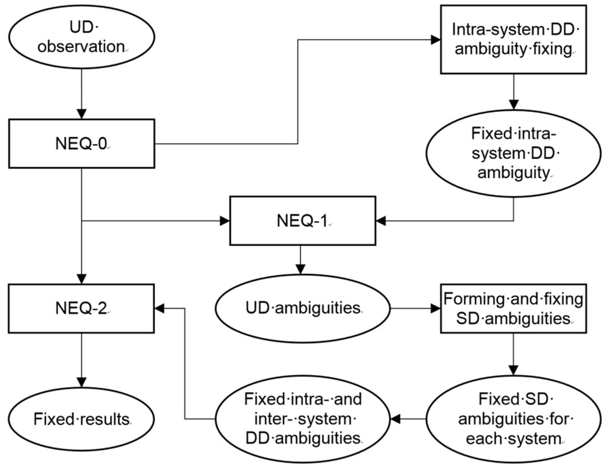
In the actual data processing, in order to improve the quality of the UD ambiguities used for the RUPD estimation, a data processing flow as shown in Figure 1 is proposed, as follows:
(1) According to Equations (1) and (7), the normal equation is formed from the UD observations for the float solution, where the satellites and receiver clocks bias are removed from the NEQ, as shown by Ge et al. [12]. As the normal UD data processing schedule, intra-system DD ambiguities are formed and fixed using the LAMBDA method [28] or decision function [29]. Following this, the normal results with the intra-system ambiguity fixed could be obtained, and a new group of UD ambiguities are also derived.
(2) With the new UD ambiguities, the RUPD estimation and the SD ambiguity fixing could be carried out following the method shown above (from Equations (10)–(13)).
(3) After that, the intra- and inter-system DD ambiguities could be formed from the fixed SD ambiguities (from Equations (14)–(16)). All these fixed DD ambiguities are applied as pseudo-observations and added to the NEQ.
(4) Finally, the fixed solutions with fixed intra- and inter-system ambiguities could be obtained.
4. Consistency between RUPD and Ambiguities
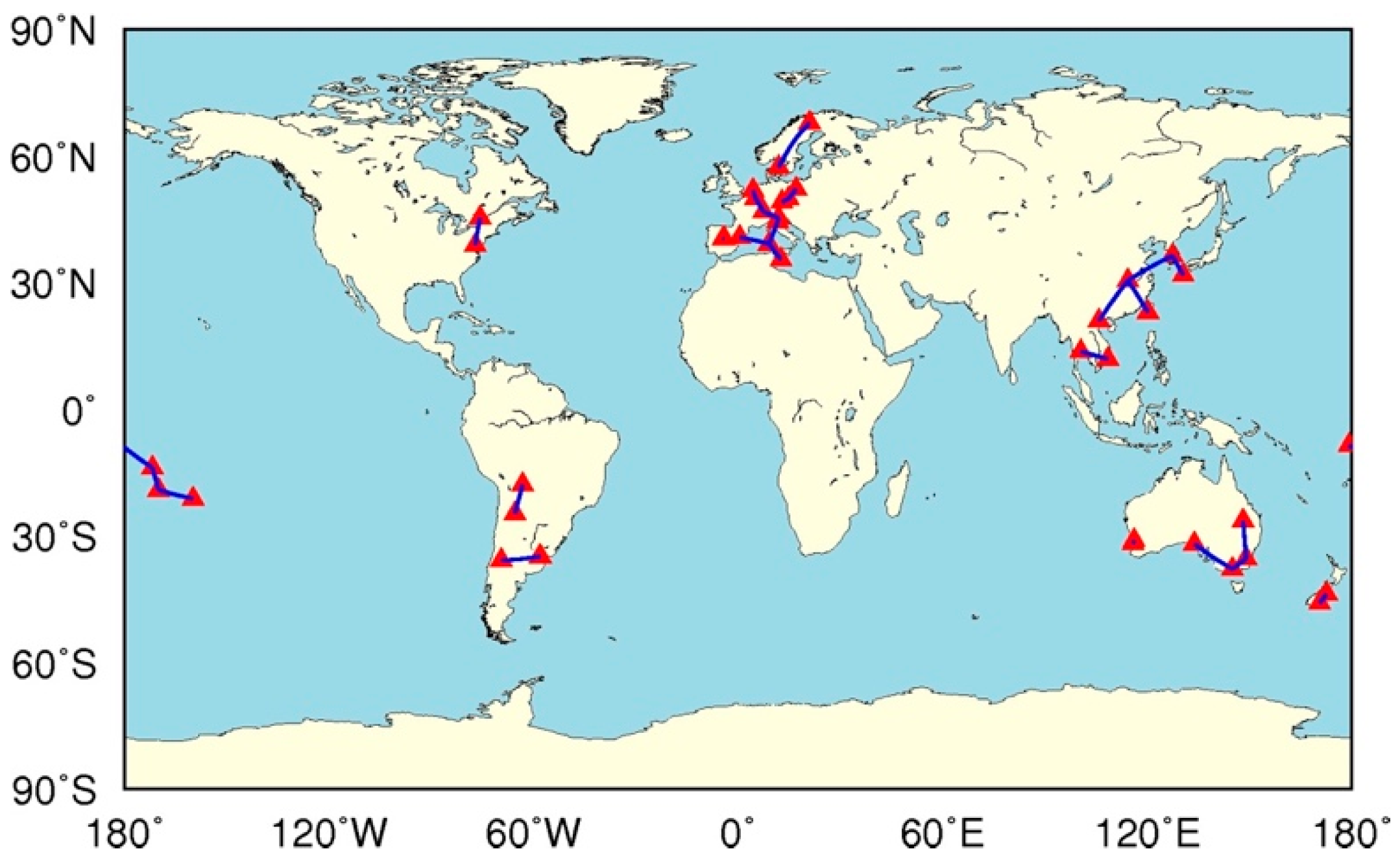
In the proposed method, the RUPD plays a very important role in the SD ambiguity fixing. It is assumed that the RUPD could be modeled as a constant if the receiver is tracking satellites continuously for each CDMA GNSS system. In order to validate this assumption, the data from about 30 baselines from MGEX network [31] ranging from several hundred meters to about 1400 km over about 14 days in 2017 are collected and used to investigate the consistency between the RUPD and ambiguities, where both GPS and Galileo data are used. First, the normal UD method is used to obtain the float solutions where the ionospheric-free combination is used; following this, the intra-system DD ambiguities are formed for the GPS and Galileo systems, respectively. After that, the DD ambiguities are used as pseudo-observations and are added to the normal equation as pseudo-observations with a weight of 1e8 [12] to obtain the fixed solutions. After that, the SD ambiguities are formed by the new UD ambiguities from the fixed solutions. Finally, the RUPD is calculated from the float SD ambiguities as a constant in each daily session. Additionally, the STD of the RUPD is also calculated for GPS and Galileo, respectively. The processing interval is 300 s. The STD of the RUPD and the residuals of the float SD ambiguities after removing the RUPD are used as an index to access the consistency between the RUPD and ambiguities. The selected baselines are shown in Figure 2. Meanwhile, in order to validate the above assumption, 4 h of data (1:00:00~1:59:30, 5:00:00~5:59:30, 13:00:00~13:59:30, 23:00:00~23:59:30) were removed for MQZG and CEDU.
The STDs of the wide-lane RUPDs (WLRUPD) are calculated for each baseline; we found most of them are less than 0.15 cycle. Taking the results of 063 days as an example, the STD of the WLRUPD for each baseline is shown in Figure 3.
It can be seen that almost all the STDs of the WLRUPDs are less than 0.15. Taking the data from all the days into consideration, the mean STD of WLRUPD is 0.084 and 0.081 for the GPS and Galileo systems, respectively. By considering the long wavelength of WL, it could be inferred that the WLRUPD derived from the methods in this research could be used for WL ambiguities fixing.
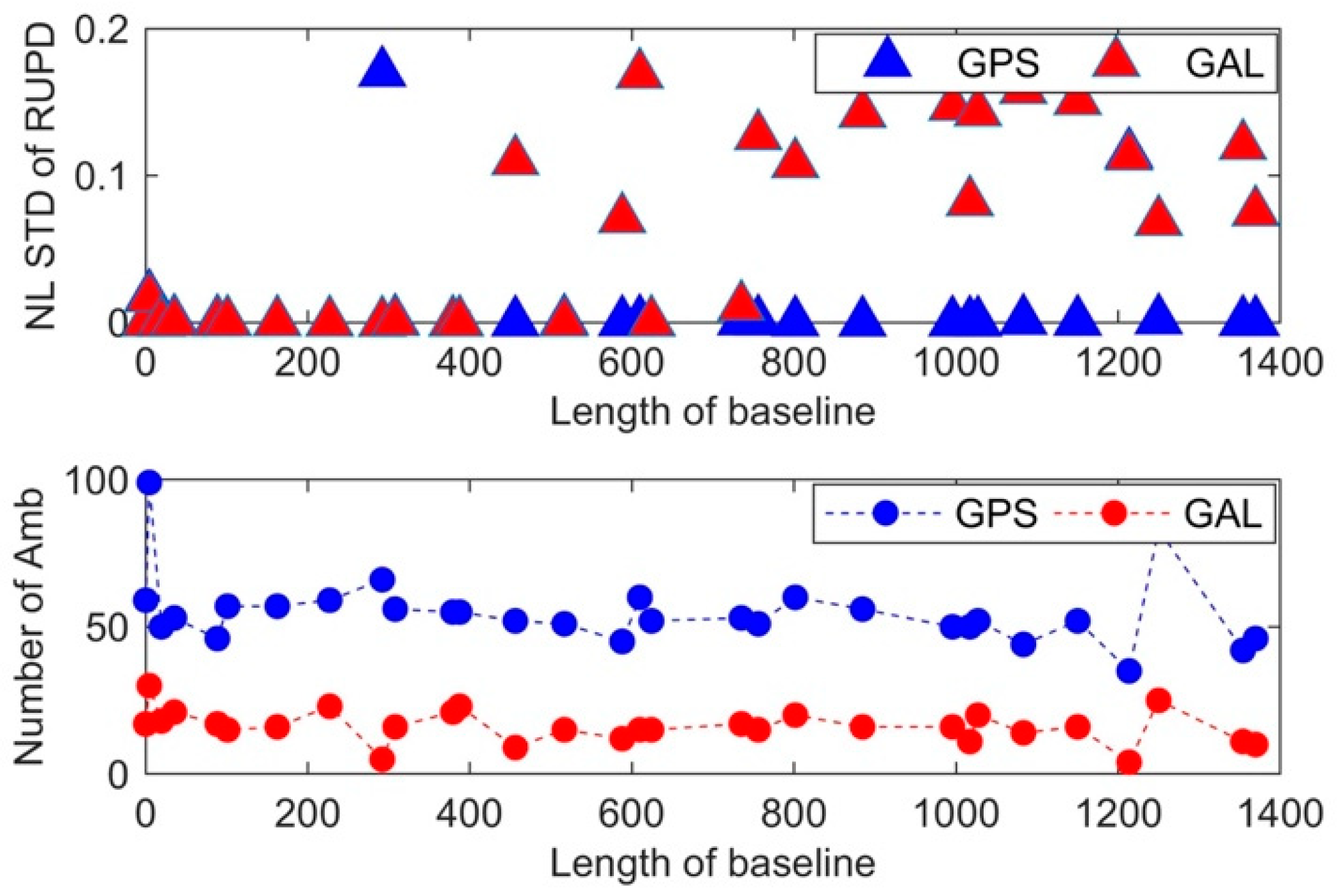
Similarly, the STD of narrow-lane RUPD (NLRUPD) is calculated with the help of fixed wide lane (WL) and UD ambiguities. As shown in Figure 4, it can be seen that the STDs of RUPDs for Galileo increase to more than 0.1 when the baseline length is larger than 500 km. One possible explanation is that the Galileo orbit products have a relative low quality compared to GPS orbits; however, a more detail investigation is needed. Therefore, those baselines with a length larger than 500 km are excluded in the following analysis for Galileo. For GPS, almost all the STDs are less than 0.03 except the two baselines DUND-MQZG and CEDU-MOBS.
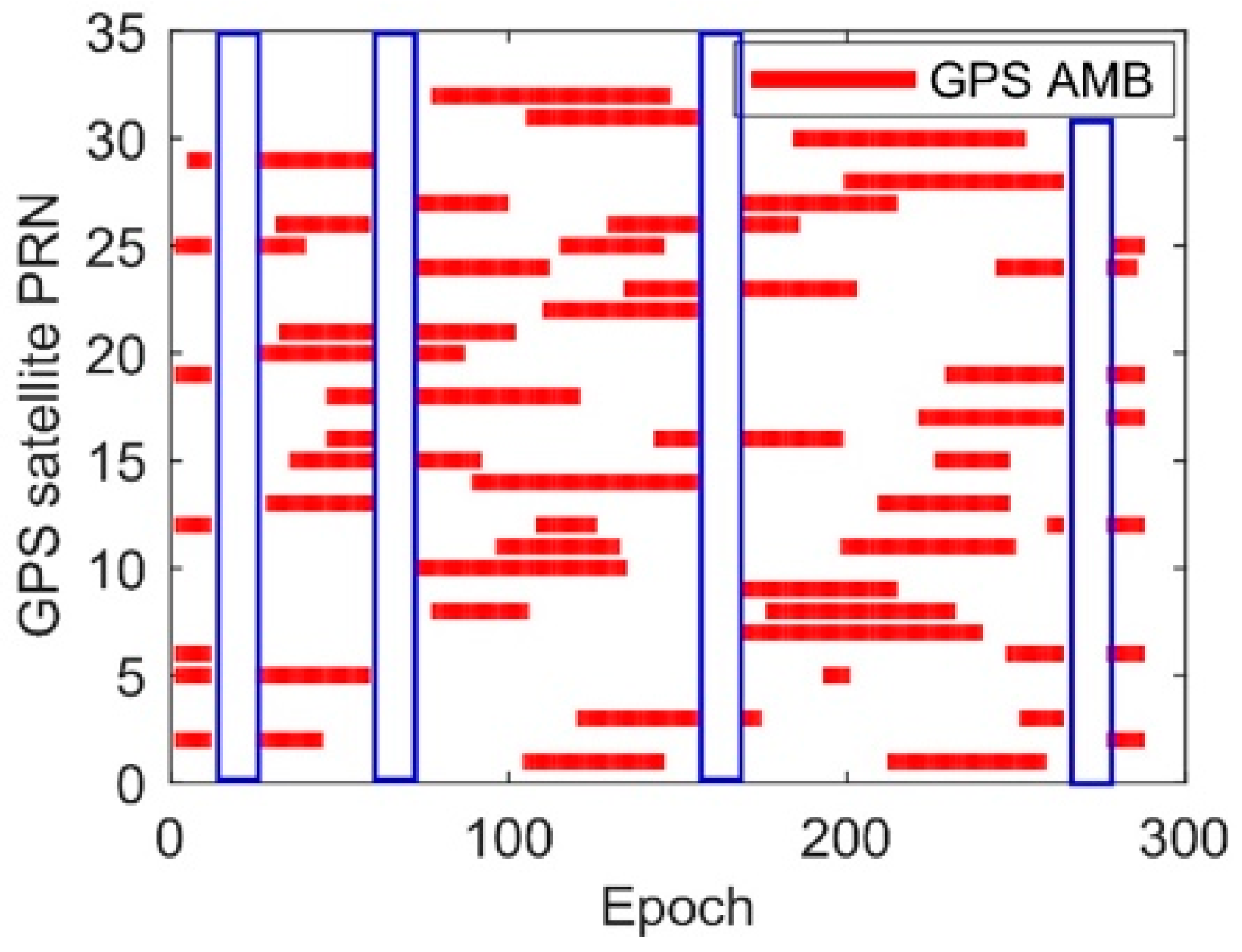
Since 4 h of data are removed for MAQZ and CEDU, as shown in Figure 5, there are 4 gaps where no satellites are observed for the above-mentioned two baselines. If the STD is calculated for each segment for the baseline DUND-MQZG, then the STDs are 0.07,0.008, 0.003, 0.008 and 0.003 for each segment, respectively. The baseline CEDU-MOBS is the same. This is because the RPUPD is highly correlated to the receiver clocks. However, the absolute receiver clocks are determined by the code observations, and the relative receiver clocks are determined by the phase observations. In other words, the absolute receiver clocks are determined by the code observations in each observing session, and the RUPD is derived based on the determined receiver clocks. It is therefore acceptable to have different RUPDs if there is a gap (no satellite is observed), which also suggests that an independent RUPD should be estimated if there is a gap.
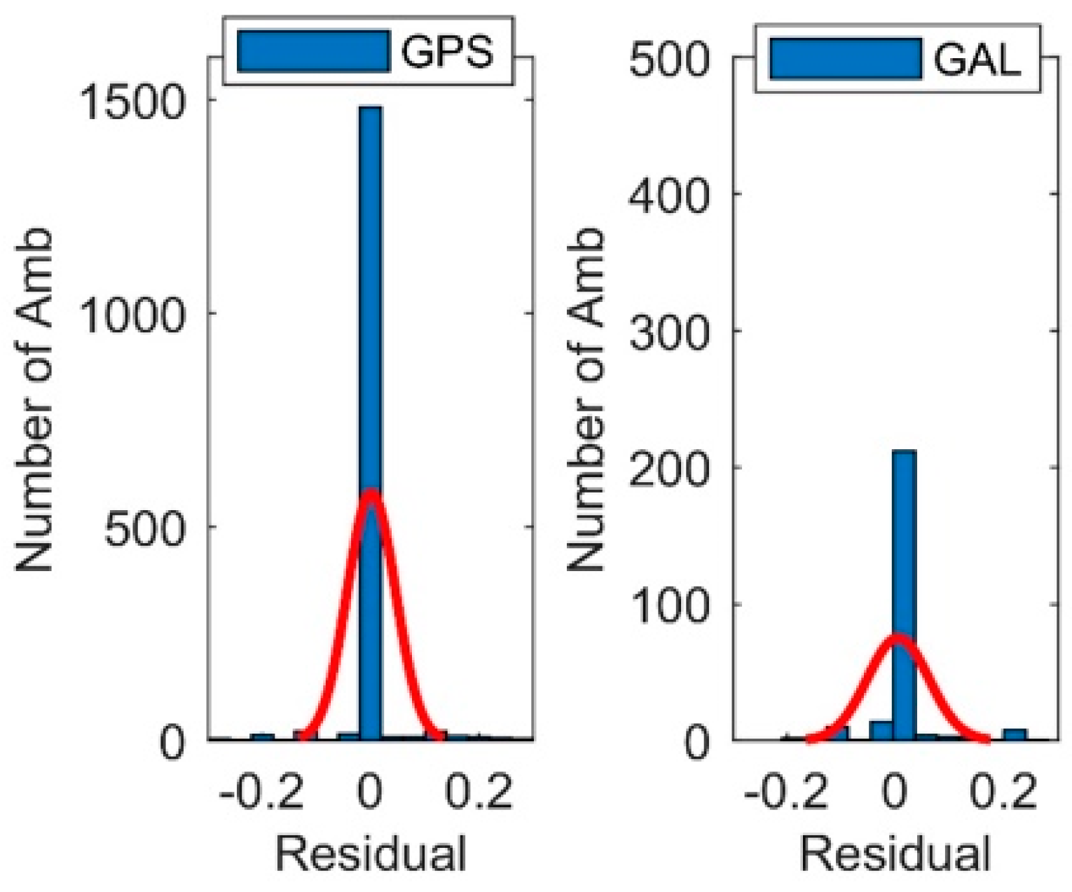
The residual of the UD ambiguities after removing the RUPD and the integer part could also be used for investigating the consistency between RUPD and ambiguities. Figure 6 shows the residual for GPS and Galileo on day 063. For Galileo, only those ambiguities from the baseline length under 500 km are used in the statistics due to the poor ambiguities fixing performance for the long baselines. Those ambiguities that cannot be fixed in the intra-system ambiguities fixing step are also included in this analysis. It can also be seen that most residuals of the SD ambiguities are close to 0, which confirmed the consistency between the RUPD and ambiguities.
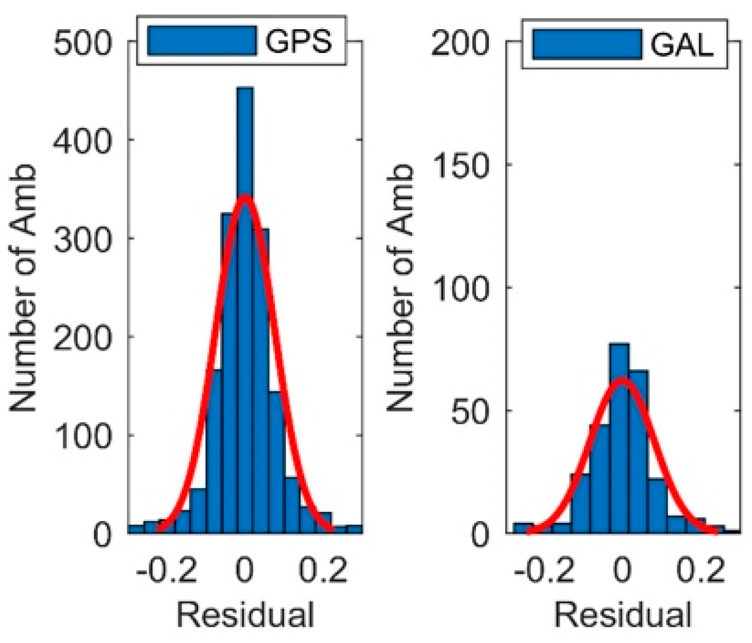
Meanwhile, the residual of the UD ambiguities without the fixed intra-system DD ambiguities applied in advance were also investigated; the result is shown in Figure 6. From Figure 6 and Figure 7, it can be inferred that applying the intra-system DD ambiguities could improve the quality of the SD ambiguities and make the residuals much closer to an integer after removing the RUPD and the integer part.
5. Inter-System Phase Bias
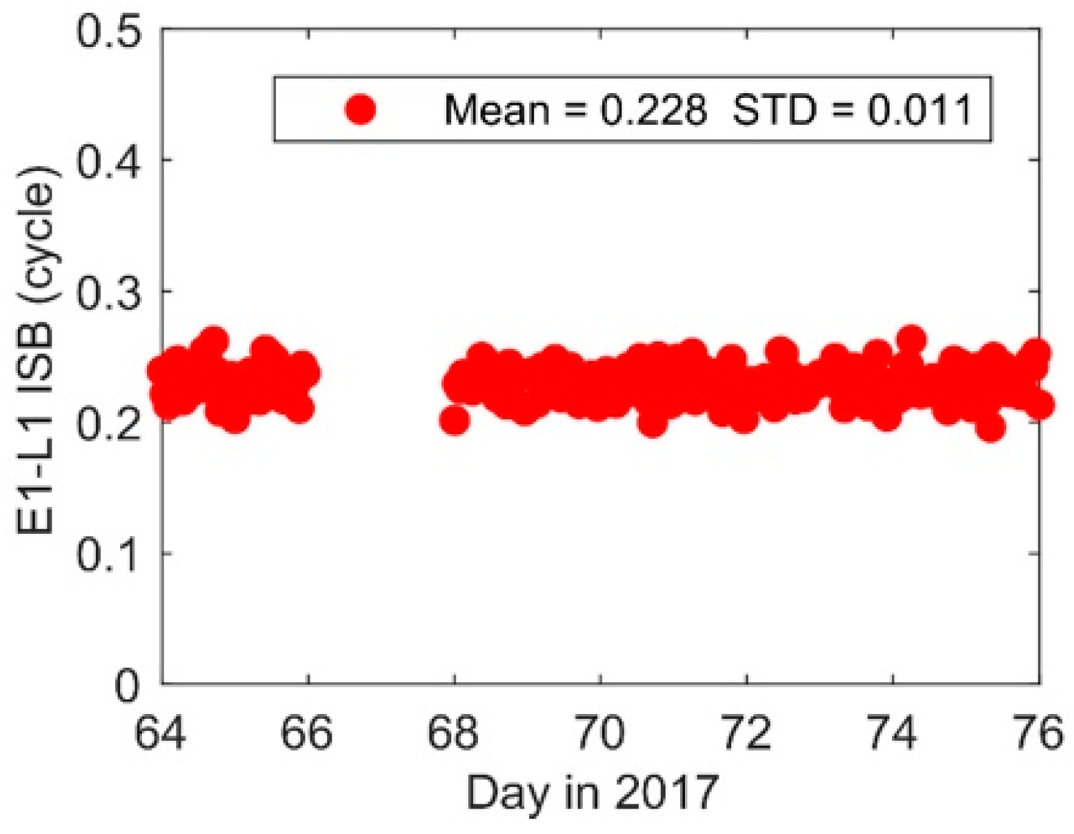
The inter-system phase bias is crucial to the inter-system ambiguity fixing. It can be guessed from Equation (16) that the difference of the RUPD of different GNSS systems could be likely regarded as the inter-system phase bias as described in the results of Paziewski and Wielgosz [17]. In order to investigate this, we selected the data of the baseline KIR8-KIRU, whose receivers are TRIMBLE NETR9 and SEPT POLARX4, respectively. According to the results by Paziewski and Wielgosz [17], the inter-system phase bias between GPS L1 and Galileo E1 is about 0.21 cycle for these two receiver types. In order to derive the inter-system bias between GPS L1 and Galileo E1, only single frequency data could be used in the baseline processing. Therefore, only a short baseline should be adopted, which is the reason why only the baseline KIR8-KIRU was selected in this experiment. Meanwhile, we divided the data into one-hour sessions and processed the data for each session independently using a least-square estimator where only GPS L1 and Galileo E1 were used. The cut-off angle is set to 7 degrees and the processing interval is 30 s. Following this, the difference between the two RUPDs was obtained and is shown in Figure 8.
The mean inter-system phase bias is 0.228 cycle and it is very stable; the STD is only 0.011 cycle. This result coincides with the results of Paziewski and Wielgosz [17]. From this result, it could be inferred that the difference between the two RUPD are likely the inter-system phase biases and may be further used to recover the integer nature of the inter-system ambiguities. Of course, more experiments are needed for further detailed investigations.
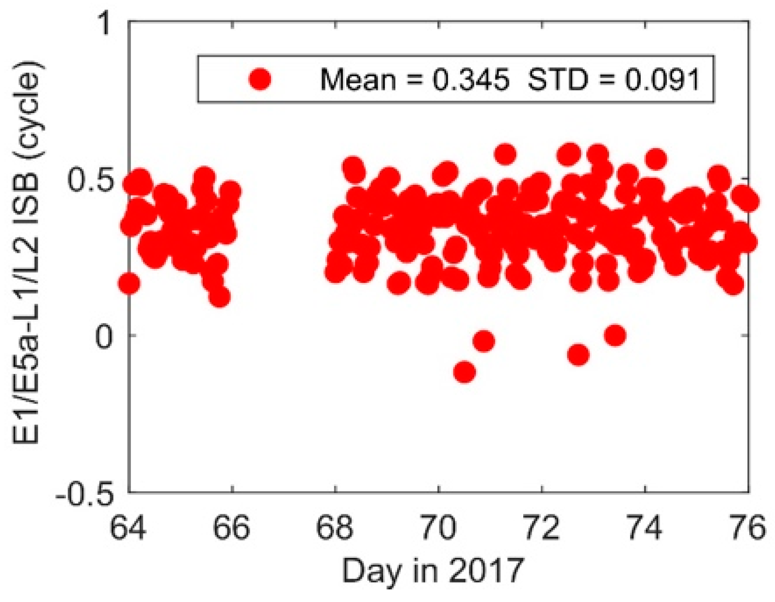
Similarly, we used ionospheric-free combinations of observations to calculate the inter-system phase bias between GPS L1/L2 and Galileo E1/E5a. Their frequencies are different. The results derived from one-hour sessions, are shown in Figure 9.
It can be seen that the mean of this inter-system phase bias is 0.345 cycle, and its STD is 0.091 which is larger than the STD for L1-E1. This it because the wavelength is only about 10 cm, which is almost half of that of L1 or E1. In order to calculate the precise inter-system phase bias, the 24-h sessions data were also processed. The results show that the average inter-system phase bias is 0.325 cycles and its STD is 0.030. These results indicate that the inter-system phase bias for the ionospheric-free combination may also be calibrated and possibly provided to others for inter-system ambiguity fixing.
6. Relative Positioning Results
In order to validate this method, the data of the baselines KIR8-KIRU(4.5 km), AGGO-LPGS (19.3 km) and NNOR-PERT (88.5 km) from days 063–076, 2017, were adopted. These data are processed with two strategies: (a) the traditional DD method where only intra-system DD observations are formed and only intra-system ambiguities are fixed; (b) the method proposed in this research, where UD observations are used and both intra-system and inter-system ambiguities are fixed. The L1 and L2 are used for the GPS while E1 and E5a are chosen for Galileo. And the ionospheric-free combination is used. Three groups of experiments are carried out with different conditions including: (1) a different cut-off angle; (2) a different challenging observation environment by simulating signal obstructions; and (3) 4 GPS satellites and all observed Galileo satellites. The processing interval was 30s and the results are shown and compared below.
6.1. Experiments with Different Cut-Off Angle
Due to the baseline KIR8-KIRU being short, we divided its experimental data into 24 one-hour sessions for each day, and each one-hour session was processed independently via strategies (a) and (b) with cut-off angles 7, 10, 20, 30, and 40 degrees; the repeatability of the baseline results was calculated and compared. The results are shown in Table 1.
It can be seen that the results of the UD observations with the fixed intra- and inter-system ambiguity (strategy b) have a better performance that those of the intra-system DD observations with the fixed intra-system ambiguity (strategy a). When the cut-off angle increases to over 20 degrees, the repeatability of the baseline components decreases very fast for strategy a; and when it reaches 40 degrees, the ambiguities cannot be fixed over several one-hour sessions. Using strategy b, the repeatability of the baseline is reduced from 20.9, 14.7, and 14.4 to 2.2, 3.0, and 8.7 mm in the east, north and vertical directions, respectively, when the cut-off angle is 30 degrees. When the cut-off angle increases to 40 degrees, there are about 20% solutions that could not be fixed for the traditional methods, a percentage reduced to 5% for the new method.
Since the ambiguity could not be fixed correctly for part of the one-hour session data using strategy a, for comparison all the data of the three baselines were divided into 6 four-hour sessions for each day. All the data for the four-hour session were reprocessed and re-statisticized. The results are shown in Table 2.
Similarly, an overall 35% and 22% improvement could be found in the horizontal and vertical directions, respectively. From the results of the baseline KIR8-KIRU, it can be seen that when the cut-off angle is 40 degrees, with strategy b, the repeatability of the baseline KIR8-KIRU is reduced from 7.1, 4.4, and 18.0 to 1.1, 1.3, and 10.8 mm in the east, north and vertical directions, respectively. Meanwhile, it can be seen that the improvement of the horizontal direction is larger than that of the vertical direction, especially when the cut-off angle is larger than 30 degrees.
6.2. Experiments with Different Simulated Signal Obstructions
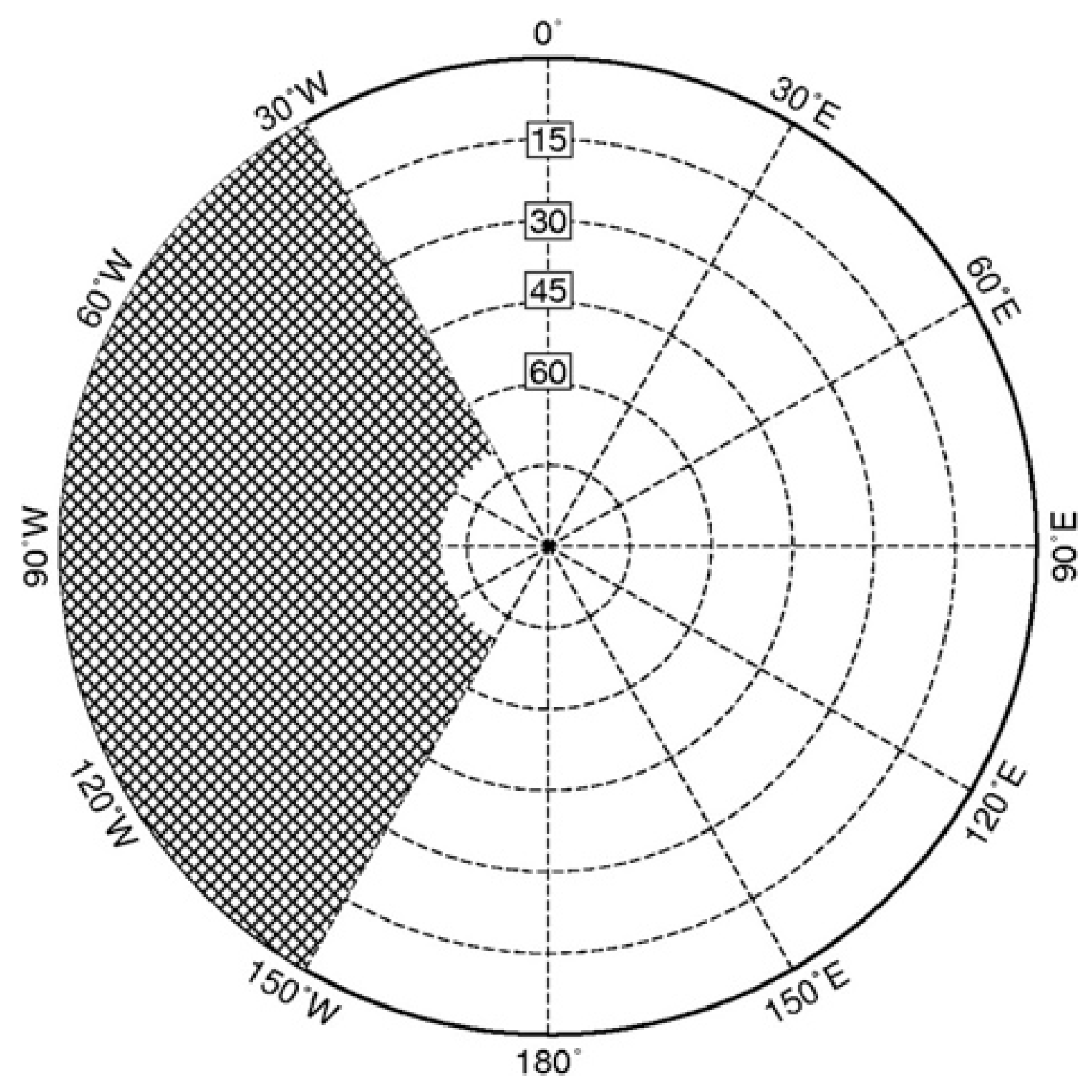
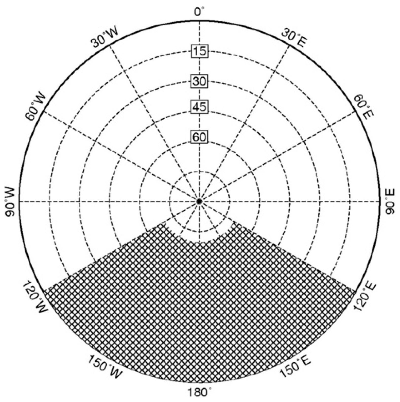
This section shows the experimental results with the different simulated signal obstructions: (1) those satellites with an elevation under 70 degrees, whose azimuths belong to [210 330], are blocked, just as shown in Figure 10, which is called scene 1 below for short; (2) those satellites with an elevation above 70 degrees, whose azimuths belong to [120 240], are blocked, as shown in Figure 11, which is called scene 2 below for short. The repeatability results of the baseline components are shown in Table 3.
From Table 3, an overall 50% improvement could be found when a part of the satellites is blocked. The baseline is shorter, and a higher accuracy could be achieved. From the results of the baseline KIRU-KIR8, it can be inferred that it may be possible to achieve an mm level for short baselines with four-hour data when there are huge obstructions located on one side of a station. Additionally, we have to note that these improvements may vary for different baselines depending on the satellite distribution and multipath effects.
6.3. Experiments with 4 GPS and All Observed Galileo Satellites
In order to further investigate the performance of this approach for short baselines when only 4 GPS satellites, along with all the available Galileo satellites, are preserved, we selected the data of the baseline KIR8-KIRU on day 063 (year 2017), and divided it into 24 one-hour sessions, for each one-hour session. Due to there being only 10 Galileo satellites being observed on this day, for each session there are only 2~5 Galileo satellites. Together with the 4 GPS satellites, there are 6 to 8 GNSS satellites for each session. The repeatability results of the baseline are shown in Table 4.
It can be seen that the result of strategy a shows an accuracy of a few centimeters; this is because the ambiguity is hard to fix for most sessions. However, even when only 4 GPS satellites were used for each session, the repeatability results of the baseline for the one-hour solutions using strategy b were 3.5, 3.7, and 8.0 mm in the east, north and vertical directions, respectively.
7. Conclusions
We studied the relative positioning methods using intra-system DD observations and using UD observations. Furthermore, we developed an approach for fixing inter-system ambiguities based on UD observations for multi-GNSS positioning. The key to this approach is the assumption that the receiver-end uncalibrated phase delay (RUPD) can be modeled as a constant if the receiver is tracking satellites continuously for each CDMA GNSS system. This assumption is validated by baselines ranging from several hundred meters to nearly 500 km. The positioning performance of this approach was also investigated using data over 12 days for the baselines KIR8-KIRU, AGGO-LPGS and NNOR-PERT via the baseline repeatability results. We found that not only the intra-system ambiguities but also the inter-system ambiguities could be fixed using this approach, no matter whether the frequencies of these GNSS systems were the same or not. The results show that the UD observations with a fixed intra- and inter-system ambiguity perform better than the DD observations with a fixed intra-system ambiguity. For the short baseline KIRU-KIR8, when the cut-off angle is 40 degrees, with the intra- and inter-system ambiguity fixed, the baseline repeatability of four-hour sessions was reduced from 7.1, 4.4, and 18.0 to 1.1, 1.3, and 10.8 mm in the east, north and vertical directions, respectively. We found that the baseline repeatability of four-hour sessions could be significantly improved when the signal obstructions were located on one side of a station. However, all these experiments were carried out in a static mode, and the performance for dynamic positioning still needs further investigations.
Author Contributions
Conceptualization, H.C., W.J. and J.L.; Methodology, H.C. and W.J.; Software, H.C.; Validation, H.C. and W.J.; Formal analysis, H.C.; Investigation, H.C.; Resources, H.C.; Data curation, H.C.; Writing—original draft preparation, H.C.; Writing—review and editing, W.J and J.L.; Visualization, H.C.; Supervision, W.J. and J.L.; Project administration, W.J.; Funding acquisition, H.C. and W.J.
Funding
This work is supported by the National Natural Science Foundation of China (NO. 41704030, 41874007 and 41525014), and the Program for Changjiang Scholars of the Ministry of Education of China.
Acknowledgments
We thank IGS MGEX for providing multi-GNSS data. We also thank the editor and three anonymous reviewers whose comments and suggestions improved the manuscript.
Conflicts of Interest
The authors declare no conflict of interest.
References
- Zumberge, J.F.; Heflin, M.B.; Jefferson, D.C.; Watkins, M.M.; Webb, F.H. Precise point positioning for the efficient and robust analysis of GPS data from large networks. J. Geophys. Res. Solid Earth 1997, 102, 5005–5017. [Google Scholar] [CrossRef] [Green Version]
- Jiang, W.P.; Liu, J.N. Study on Application of GPS in the Geheyan Dam Deformation Monitoring. Wuhan Univ. J. Nat. Sci. 1998, 23, 48–49. [Google Scholar]
- Chen, H.; Xiao, Y.; Jiang, W.; Zhou, X.; Liu, H. An improved method for multi-GNSS baseline processing using single difference. Adv. Space Res. 2019, in press. [Google Scholar] [CrossRef]
- Yang, Y.X.; Li, J.L.; Xu, J.Y.; Tang, J.; Guo, H.; He, H. Contribution of the compass satellite navigation system to global PNT users. Chin. Sci. Bull. 2011, 56, 2813–2819. [Google Scholar] [CrossRef]
- European Union. European GNSS (Galileo) Open Service Signal in Space: Interface Control Document, OS SIS ICD. 2010. Available online: https://ec.europa.eu/docsroom/documents/11870/attachments/1/translations/en/renditions/native (accessed on 14 January 2019).
- Schönemann, E.; Becker, M.; Springer, T. A new approach for GNSS analysis in a multi-GNSS and multi-signal environment. J. Geod. Sci. 2011, 1, 204–214. [Google Scholar] [CrossRef]
- Li, X.; Ge, M.; Dai, X.; Ren, X.; Fritsche, M.; Wickert, J.; Schuh, H. Accuracy and reliability of multi-GNSS real-time precise positioning: GPS, GLONASS, BeiDou, and Galileo. J. Geod. 2015, 89, 607–635. [Google Scholar] [CrossRef] [Green Version]
- Odolinski, R.; Teunissen, P.; Odijk, D. Combined BDS, Galileo, QZSS and GPS single-frequency RTK. GPS Solut. 2014, 19, 151–163. [Google Scholar] [CrossRef]
- Xu, G. GPS data processing with equivalent observation equations. GPS Solut. 2002, 6, 28–33. [Google Scholar] [CrossRef]
- Schaffrin, B.; Bock, Y. A unified scheme for processing GPS dual-band phase observations. Bull. Géodésique 1988, 62, 142–160. [Google Scholar] [CrossRef]
- Ge, M.; Gendt, G.; Rothacher, M.; Shi, C.; Liu, J. Resolution of GPS carrier-phase ambiguities in precise point positioning (PPP) with daily observations. J. Geod. 2008, 82, 389–399. [Google Scholar] [CrossRef]
- Ge, M.; Gendt, G.; Dick, G.; Zhang, P.F.; Rothacher, M. A new data processing strategy for huge GNSS global networks. J. Geod. 2006, 80, 199–203. [Google Scholar] [CrossRef]
- Julien, O.; Alves, P.; Cannon, E.; Zhang, W. A tightly coupled GPS/Galileo combination for improved ambiguity resolution. In Proceedings of the ENC-GNSS 2003, Graz, Austria, 22–25 April 2003. [Google Scholar]
- Odijk, D.; Teunissen, P. Characterization of between-receiver GPS-Galileo inter-system biases and their effect on mixed ambiguity resolution. GPS Solut. 2013, 17, 521–533. [Google Scholar] [CrossRef]
- Odijk, D.; Teunissen, P. Estimation of differential inter-system biases between the overlapping frequencies of GPS, Galileo, BeiDou and QZSS. In Proceedings of the 4th International Colloquium Scientific and Fundamental Aspects of the Galileo Programme 2013, Prague, Czech Republic, 4–6 December 2013. [Google Scholar]
- Odijk, D.; Teunissen, P.; Khodabandeh, A. Galileo IOV RTK positioning: Standalone and combined with GPS. Surv. Rev. 2014, 46, 267–277. [Google Scholar] [CrossRef]
- Paziewski, J.; Wielgosz, P. Accounting for Galileo-GPS inter- system biases in precise satellite positioning. J. Geod. 2015, 89, 81–93. [Google Scholar] [CrossRef]
- Gao, W.; Gao, C.; Pan, S.; Meng, X.; Xia, Y. Inter-System Differencing between GPS and BDS for Medium-Baseline RTK Positioning. Remote Sens. 2017, 9, 948. [Google Scholar] [CrossRef]
- Tian, Y.; Ge, M.; Neitzel, F.; Zhu, J. Particle filter-based estimation of inter-system phase bias for real-time integer ambiguity resolution. GPS Solut. 2016, 21, 949–961. [Google Scholar] [CrossRef]
- Tian, Y.; Liu, Z.; Ge, M.; Neitzel, F. Determining inter-system bias of GNSS signals with narrowly spaced frequencies for GNSS positioning. J. Geod. 2018, 92, 873–887. [Google Scholar] [CrossRef]
- Khodabandeh, A.; Teunissen, P.J.G. PPP-RTK and inter-system biases: The ISB look-up table as a means to support multi-system PPP-RTK. J. Geod. 2016, 90, 837–851. [Google Scholar] [CrossRef]
- Geng, J.; Li, X.; Zhao, Q.; Li, G. Inter-system PPP ambiguity resolution between GPS and BeiDou for rapid initialization. J. Geod. 2018, 1–16. [Google Scholar] [CrossRef]
- Xiao, Y.; Jiang, W.; Chen, H.; Yuan, P.; Xi, R. Research and realization of deformation monitoring algorithm with millimeter level precision based on BeiDou Navigation Satellite System. Wuhan Univ. J. Nat. Sci. 2016, 45, 16–21. [Google Scholar]
- Salazar, D.; Hernandez-Pajares, M.; Juan, J.M.; Sanz, J. GNSS data management and processing with the GPSTk. GPS Solut. 2010, 14, 293–299. [Google Scholar] [CrossRef]
- Wang, M.; Cai, H.; Pan, Z. BDS/GPS relative positioning for long baseline with undifferenced observations. Adv. Space Res. 2015, 55, 113–124. [Google Scholar] [CrossRef]
- Liu, J.; Ge, M. PANDA software and its preliminary result of positioning and orbit determination. Wuhan Univ. J. Nat. Sci. 2003, 8, 603–609. [Google Scholar]
- Yi, W.; Song, W.; Lou, Y.; Shi, C.; Yao, Y.; Guo, H.; Chen, M.; Wu, J. Improved method to estimate undifferenced satellite fractional cycle biases using network observations to support PPP ambiguity resolution. GPS Solut. 2017, 21, 1369–1378. [Google Scholar] [CrossRef]
- Teunissen, P.J.G. The least-squares ambiguity decorrelation adjustment: A method for fast GPS integer ambiguity estimation. J. Geod. 1995, 70, 65–82. [Google Scholar] [CrossRef]
- Dong, D.; Bock, Y. Global positioning system network analysis with phase ambiguity resolution applied to crustal deformation studies in California. J. Geophys. Res. Solid Earth 1989, 94, 3949–3966. [Google Scholar] [CrossRef]
- Blewitt, G. Carrier phase ambiguity resolution for the global positioning system applied to geodetic baselines up to 2,000 km. J. Geophys. Res. Solid Earth 1989, 94, 10187–10203. [Google Scholar] [CrossRef]
- Montenbruck, O.; Steigenberger, P.; Prange, L.; Deng, Z.; Zhao, Q.; Perosanz, F.; Romero, I.; Noll, C.; Stürze, A.; Weber, G.; et al. The Multi-GNSS Experiment (MGEX) of the International GNSS Service (IGS)—Achievements, Prospects and Challenges. Adv. Space Res. 2017, 59, 1671–1697. [Google Scholar] [CrossRef]
Figure 1.
The procedure of intra- and inter-system ambiguity fixing in the actual data processing.

Figure 2.
The selected baseline. GPS and Galileo are observed for each baseline.

Figure 3.
STD and number of ambiguities used for WLRUPD.

Figure 4.
The STD and number of ambiguities used for NLRUPD.

Figure 5.
Observation time of all satellites for the baselines DUND-MQZG and CEDU-MOBS on day 063, 2017.
Figure 5.
Observation time of all satellites for the baselines DUND-MQZG and CEDU-MOBS on day 063, 2017.

Figure 6.
Residuals of the SD ambiguity after removing the RUPD and the integer part with the intra-system DD ambiguities fixed.
Figure 6.
Residuals of the SD ambiguity after removing the RUPD and the integer part with the intra-system DD ambiguities fixed.

Figure 7.
Residuals of the SD ambiguity after removing the RUPD and the integer part without the intra-system DD ambiguities fixed.
Figure 7.
Residuals of the SD ambiguity after removing the RUPD and the integer part without the intra-system DD ambiguities fixed.

Figure 8.
Inter-system phase bias derived for GPS and Galileo L1-E1 for KIR8 and KIRU.

Figure 9.
Inter-system phase bias derived for GPS and Galileo L1/L2-E1/E5a for KIR8 and KIRU.

Figure 10.
Simulated obstructions. The shadow part shows that those satellites with an elevation under 70 degrees, whose azimuths belong to [210 330], are blocked.
Figure 10.
Simulated obstructions. The shadow part shows that those satellites with an elevation under 70 degrees, whose azimuths belong to [210 330], are blocked.

Figure 11.
Simulated obstructions. The shadow part shows that those satellites with an elevation above 70 degrees, whose azimuths belong to [120 240], are blocked.
Figure 11.
Simulated obstructions. The shadow part shows that those satellites with an elevation above 70 degrees, whose azimuths belong to [120 240], are blocked.


Table 1.
The repeatability of the baseline KIR8-KIRU with different cut-off angles over one-hour sessions.
Table 1.
The repeatability of the baseline KIR8-KIRU with different cut-off angles over one-hour sessions.
| Cutoff Angle | Intra-System DD Observations with the Fixed Intra-System Ambiguity (mm) (Strategy a) | UD Observations with the Fixed Intra- and Inter-System Ambiguity (mm) (Strategy b) | ||||
|---|---|---|---|---|---|---|
| East | North | Up | East | North | Up | |
| 7 | 7.0 | 6.0 | 8.8 | 1.9 | 2.5 | 6.4 |
| 10 | 7.0 | 5.9 | 8.5 | 2.1 | 2.6 | 6.5 |
| 20 | 8.0 | 7.0 | 8.2 | 1.9 | 2.4 | 6.7 |
| 30 | 20.9 | 14.7 | 14.4 | 2.2 | 3.0 | 8.7 |
| 40 | 315.7 | 86.8 | 94.2 | 43.0 | 21.0 | 22.8 |
Table 2.
The repeatability of the baseline components with different cut-off angles over four-hour sessions.
Table 2.
The repeatability of the baseline components with different cut-off angles over four-hour sessions.
| Baselines | Cutoff Angle (Degree) | Intra-System DD Observations the with Fixed Intra-System Ambiguity (mm) (Strategy a) | UD Observations with the Fixed Intra- and Inter-System Ambiguity (mm) (Strategy b) | ||||
|---|---|---|---|---|---|---|---|
| East | North | Up | East | North | Up | ||
| KIR8-KIRU | 7 | 1.9 | 1.3 | 2.3 | 1.1 | 0.8 | 2.2 |
| 10 | 1.7 | 1.2 | 2.4 | 1.1 | 0.8 | 2.3 | |
| 20 | 2.2 | 1.1 | 3.0 | 1.0 | 0.5 | 2.6 | |
| 30 | 5.6 | 1.1 | 6.0 | 0.8 | 1.3 | 4.2 | |
| 40 | 7.1 | 4.4 | 18.0 | 1.1 | 1.3 | 10.8 | |
| AGGO-LPGS | 7 | 2.1 | 6.3 | 16.7 | 2.0 | 4.0 | 12.2 |
| 10 | 2.1 | 6.2 | 16.6 | 2.3 | 4.1 | 12.2 | |
| 20 | 3.6 | 5.5 | 19.7 | 1.6 | 3.5 | 10.1 | |
| 30 | 4.9 | 5.9 | 27.2 | 2.2 | 2.9 | 22.1 | |
| 40 | 7.5 | 7.6 | 60.8 | 2.3 | 2.1 | 56.6 | |
| NNOR-PERT | 7 | 1.9 | 2.7 | 12.9 | 1.8 | 3.3 | 9.6 |
| 10 | 1.9 | 3.0 | 12.4 | 2.1 | 3.2 | 10.1 | |
| 20 | 2.9 | 3.0 | 16.8 | 2.5 | 2.3 | 17.9 | |
| 30 | 6.0 | 5.2 | 36.8 | 2.5 | 2.3 | 20.1 | |
| 40 | 7.1 | 7.4 | 78.0 | 3.7 | 3.3 | 55.5 | |
Table 3.
Repeatability of the baseline KIR8-KIRU with different simulated signal obstructions over four-hour sessions.
Table 3.
Repeatability of the baseline KIR8-KIRU with different simulated signal obstructions over four-hour sessions.
| Baselines | Intra-System DD Observations with the Fixed Intra-System Ambiguity (mm) (Strategy a) | UD Observations with the Fixed Intra- and Inter-System Ambiguity (mm) (Strategy b) | |||||
|---|---|---|---|---|---|---|---|
| East | North | Up | East | North | Up | ||
| KIRU-KIR8 | Scene 1 | 12.5 | 4.1 | 14.0 | 6.0 | 1.1 | 9.0 |
| Scene 2 | 5.9 | 9.0 | 13.6 | 2.4 | 2.3 | 5.5 | |
| AGGO-LPGS | Scene 1 | 16.1 | 7.3 | 21.6 | 2.4 | 3.3 | 11.7 |
| Scene 2 | 5.1 | 12.2 | 26.6 | 4.9 | 5.5 | 15.1 | |
| NNOR-PERT | Scene 1 | 18.9 | 6.0 | 32.4 | 5.6 | 3.5 | 23.9 |
| Scene 2 | 10.9 | 13.1 | 41.2 | 8.1 | 5.9 | 28.5 | |
Table 4.
The repeatability of the baseline with all the observed Galileo and 4 GPS satellites over one-hour sessions.
Table 4.
The repeatability of the baseline with all the observed Galileo and 4 GPS satellites over one-hour sessions.
| The Fixed Intra-System Ambiguity (mm) (Strategy a) | UD Observations with the Fixed Intra- and Inter-System Ambiguity (mm) (Strategy b) | |||||
|---|---|---|---|---|---|---|
| East | North | Up | East | North | Up | |
| All observed Galileo satellites, along with the 4 GPS satellites | 41.2 | 25.9 | 22.2 | 3.5 | 3.7 | 8.0 |
© 2019 by the authors. Licensee MDPI, Basel, Switzerland. This article is an open access article distributed under the terms and conditions of the Creative Commons Attribution (CC BY) license (http://creativecommons.org/licenses/by/4.0/).
Share and Cite
MDPI and ACS Style
Chen, H.; Jiang, W.; Li, J. Multi-GNSS Relative Positioning with Fixed Inter-System Ambiguity. Remote Sens. 2019, 11, 454. https://0-doi-org.brum.beds.ac.uk/10.3390/rs11040454
AMA Style
Chen H, Jiang W, Li J. Multi-GNSS Relative Positioning with Fixed Inter-System Ambiguity. Remote Sensing. 2019; 11(4):454. https://0-doi-org.brum.beds.ac.uk/10.3390/rs11040454
Chicago/Turabian StyleChen, Hua, Weiping Jiang, and Jiancheng Li. 2019. "Multi-GNSS Relative Positioning with Fixed Inter-System Ambiguity" Remote Sensing 11, no. 4: 454. https://0-doi-org.brum.beds.ac.uk/10.3390/rs11040454
Note that from the first issue of 2016, this journal uses article numbers instead of page numbers. See further details here.