Photon-Counting Lidar: An Adaptive Signal Detection Method for Different Land Cover Types in Coastal Areas

Abstract

Airborne or space-borne photon-counting lidar can provide successive photon clouds of the Earth’s surface. The distribution and density of signal photons are very different because different land cover types have different surface profiles and reflectance, especially in coastal areas where the land cover types are various and complex. A new adaptive signal photon detection method is proposed to extract the signal photons for different land cover types from the raw photons captured by the MABEL (Multiple Altimeter Beam Experimental Lidar) photon-counting lidar in coastal areas. First, the surface types with 30 m resolution are obtained via matching the geographic coordinates of the MABEL trajectory with the NLCD (National Land Cover Database) datasets. Second, in each along-track segment with a specific land cover type, an improved DBSCAN (Density-Based Spatial Clustering of Applications with Noise) algorithm with adaptive thresholds and a JONSWAP (Joint North Sea Wave Project) wave algorithm is proposed and integrated to detect signal photons on different surface types. The result in Pamlico Sound indicates that this new method can effectively detect signal photons and successfully eliminate noise photons below the water level, whereas the MABEL result failed to extract the signal photons in vegetation segments and failed to discard the after-pulsing noise photons. In the Atlantic Ocean and Pamlico Sound, the errors of the RMS (Root Mean Square) wave height between our result and in-situ result are −0.06 m and 0.00 m, respectively. However, between the MABEL and in-situ result, the errors are −0.44 m and −0.37 m, respectively. The mean vegetation height between the East Lake and Pamlico Sound was also calculated as 15.17 m using the detecting signal photons from our method, which agrees well with the results (15.56 m) from the GFCH (Global Forest Canopy Height) dataset. Overall, for different land cover types in coastal areas, our study indicates that the proposed method can significantly improve the performance of the signal photon detection for photon-counting lidar data, and the detected signal photons can further obtain the water levels and vegetation heights. The proposed approach can also be extended for ICESat-2 (Ice, Cloud, and land Elevation Satellite-2) datasets in the future.

1. Introduction

Equipped with more sensitive sensors (Gm-APDs (Geiger mode avalanche photodiodes) or PMTs (photomultipliers)), photon-counting lidar can respond to the presence of return photons rather than capturing the return waveforms of traditional lidar [1,2]. Benefitting from photon-counting sensors, the lasers of photon-counting lidar achieve lower energy (several tens of μJ), higher repetition rate (several KHz) and lower divergence (a few tens of μrad) compared to traditional lidar (several tens of mJ, a few tens of Hz, and a few mrad). After the ICESat (ice, cloud, and land elevation satellite) traditional laser altimeter, the ICESat-2 photon-counting lidar will measure the ice sheet elevation, sea ice freeboard, vegetation canopy, and ocean surface, and provide successive photon clouds of the Earth’s surface with smaller laser footprints and higher spatial density (an along-track footprint interval of 0.7 m) [3,4]. Prior to the launch, an airborne photon-counting lidar, i.e., MABEL (Multiple Altimeter Beam Experimental Lidar), was used as a high-altitude prototype for the ICESat-2 lidar [5].

Due to the lower transmitted laser energy, the mean signal photons per shot varies from 0.1 to 10 photons [4,6]. The return-signal photon clouds of the surface are very noisy and suffer from background noise, backscatter noise, detector dark noise, and after-pulsing noise photons [7]. In the daytime, the solar background noise rate is approximately several MHz, which makes the number of background noise photons exceed the number of signal photons within the range gate. Compared to background noise, the detector dark noise rate is only several KHz and can be neglected [8]. The backscatter effect arising from clouds and aerosols and the after-pulsing detector effect introduce noise photons into the signal photons above and below the ground surface, respectively [9]. To use photon clouds for monitoring environmental changes, weak laser signal photons should be precisely extracted from the noisy raw datasets of photon-counting lidar.

Many methods have been proposed to successfully process the laser point clouds captured by full waveform lidars [10,11], especially for Mallet’s achievements on waveform processing for different targets [12,13]. However, most methods cannot be used to effectively detect the signal photons from the much noisy raw photons captured by photon-counting lidars because the raw photons from a photon-counting lidar correspond to the energy at only a single photon level (approximately 1000 repeated measurements are needed to construct an accumulated waveform), whereas the points from a full waveform lidar correspond to the energy at thousands of photons level (these photons can directly construct a return waveform). Apart from the ice sheet surface (because ice sheet surface is very smooth and flat and can be assumed as identical in an area of hundred-meter size), 1000 repeated measurements will correspond to different Earth’s surfaces (a high-altitude aircraft will pass tens of meters and a low earth orbit satellite will pass a few hundred meters during the time duration of 1000 repeated measurements). In addition, a photon-counting lidar suffers from the dead-time effect and after-pulsing effect, which significantly influence the distribution of captured photon clouds. The dead-time effect is that after a response to a received photon, a photon-counting detector needs a time duration to recover. In the recovering time duration (i.e., the dead-time), the photon-counting detector will not respond to any received photons. The after-pulsing effect is that if a photon-counting detector is triggered by incidence photons, the photon-counting detector may be self-triggered after its response to these incidence photons (normally tens of ns later). If the incidence energy is larger (with more incidence photons), the photon-counting detector will be more likely to be self-triggered [7].

Many signal detecting methods for photon-counting lidar data have been developed. First, general signal photon detection methods were proposed and used for simulated datasets or the raw datasets captured by photon-counting lidar in labs, e.g., the correlation range receiver (CRR) method [14] and adaptive ellipsoid searching (AES) method [15]. For the MABEL raw datasets, a surface-finding algorithm was proposed to detect surface profiles from the raw data captured in regions of sea ice and ice sheets [16,17,18]. For datasets of ice sheet surfaces, an adaptive window size with a recursive nearest-neighbor analysis was proposed for discarding noise photons [19]. For datasets in urban and forested regions, an adaptive ellipsoid searching filter [20], an adaptive density-based model [21], the contour active models [22], the spatial statistical and discrete mathematical concepts [8], and a noise removal algorithm based on localized statistical analysis [23] were derived to detect the surface profiles. For the datasets of ocean surfaces, a surface detection method was proposed based on the wave spectrum and nonlinear least-squares fitting [9].

In coastal areas, the raw photon clouds are more sophisticated because a variety of Earth’s surface types (e.g., open sea, shoals, wetlands, banks, sandy beaches, and docks) correspond to different surface profiles and reflectance. There is not a specific method to detect the various types of surface profiles. Kwok proposed a method to identify and detect sea ice and open water in the Arctic [24]. However, this surface finding method cannot effectively detect the surface profiles of wetlands. To detect the surface profiles of different types from the MABEL raw datasets in coastal areas, a new method is derived in this study. First, the surface types of the MABEL trajectory with a resolution of 30 m are obtained via matching the geographic coordinates of the MABEL trajectory with the geographic coordinates in NLCD (National Land Cover Database). Second, an improved DBSCAN (Density-Based Spatial Clustering of Applications with Noise) algorithm with adaptive thresholds and a JONSWAP (Joint North Sea Wave Project) spectrum algorithm are integrated to detect surface profiles of different types. The Pamlico Sound (in North Carolina, USA), where the MABEL lidar flew over the open sea, sound water, wetlands, shoals, banks, sandy beaches, and docks, is selected as the study area and surface profiles of different types are extracted via this new method.

2. Study Area and Datasets

2.1. Study Area and the In-Situ Data

Pamlico Sound in North Carolina is the largest lagoon along the East Coast of the United States (with a length of 130 km and width of 24 to 48 km), and it is the second largest estuary in the United States (with over 7500 km² of open water) (from https://en.wikipedia.org/wiki/Pamlico_Sound). In the east, the Outer Banks separate the Pamlico Sound from the Atlantic Ocean. In the west, the area is covered by various vegetations (e.g., shrub/scrub, cultivated crops, woody wetlands, and herbaceous wetlands). Many sandy barrier islands are inside the Pamlico Sound. According to the NLCD 2011 products, there are seven types of land cover near the Pamlico Sound (i.e., open water, mixture of constructed materials and vegetation, barren land, shrub/scrub, cultivated crops, woody wetlands, and herbaceous wetlands). Figure 1 shows the map of the Pamlico Sound and its location in the USA.

In this area, the in-situ data of two nearby stations provided by NOAA (National Oceanic and Atmospheric Administration) are used to evaluate the calculated results (i.e., the water level and RMS (Root Mean Square) wave height). The Oregon Inlet Marina Station (ID: 8652587) is inside the sound, and Duck Station (ID: 8651370) is on a platform above the Atlantic Ocean. These stations provide historical datasets including mean sea level and wind speed every six minutes, and the data can be downloaded from the website (https://www.co-ops.nos.noaa.gov). The water level heights of these stations are on the benchmark of NAVD88 (North American Vertical Datum of 1988) [25].

2.2. National Land Cover Database (NLCD)

The NLCD, supported by the MultiResolution Land Characteristics (MRLC) Consortium (http://www.mrlc.gov), is a widely used national scale land cover product [26]. The NLCD has 16 types of land cover and related information for 2001, 2006 and 2011. In the NLCD 2011 product, every type of land cover has a 30-m spatial resolution (i.e., the pixel size of Landsat imagery). The NLCD project was conducted to monitor the land cover and its change over time for various applications in ecology, climate change, land management and environmental planning. Landsat 5 Thematic Mapper (TM) imagery was used to generate the NLCD 2011 products. All Landsat images were acquired from the United States Geological Survey (USGS) Earth Resources Observation and Science (EROS) Center Landsat archive with radiometrical and geometrical calibration. All the production is geo-registered to the Albers Equal Area projection grid and resampled to a 30-m spatial resolution. The single-date overall accuracy of the NLCD 2011 products is 88% at level I and 82% at level II [27].

2.3. MABEL Datasets

The MABEL photon-counting lidar that was flown aboard the ER-2 and Proteus aircraft at an altitude of 20 km captured signal and noise photons (i.e., the raw datasets) and recorded the corresponding time tags [17]. The MABEL lidar has a transmitting laser pulse of 0.65 ns (1 sigma), a laser divergence of 0.1 mrad (the laser footprint is 2 m in diameter at 20 km altitude), a mean received energy of several 10⁻¹⁹ J (~1 photons @ 532 nm and 1064 nm), and a laser pulse repetition rate of 5~25 kHz. In the study area, the MABEL was at a laser repetition rate of 5 kHz and at an aircraft ground speed of approximately 215 m/s corresponding to an interval of 4 cm between contiguous laser pulses along the track. Up to 16 channels for the 532 nm green laser and eight channels for the 1064 nm near-infrared laser with different viewing angles are available for the MABEL, and each channel can independently and separately capture data photons [2]. For all available channels, every MABEL dataset records the raw data photons for a 1-min duration of the along-track flight.

The MABEL datasets used in this study were captured on 21/09/2012 near the Pamlico Sound (North Carolina, USA) and can be downloaded from the NASA ICESat-2 website (https://icesat.gsfc.nasa.gov/icesat2/data/mabel/data/browse/index.html). The weather was very clear at that time. The MABEL trajectory was from the ocean (east) to the land (west) in the study area as illustrated in Figure 1 (using red lines). In the MABEL Level 2A dataset, each photon represents the WGS84 coordinate frame and has a unique geographic coordinate of latitude, longitude and elevation. After the ranging corrections and systematic bias calibration, the MABEL signal photons are estimated to have a vertical accuracy from 13 to 24 cm (1-sigma) [28].

2.4. Global Forest Canopy Height Data

The Global Forest Canopy Height (GFCH) datasets are used for the comparison of the vegetation height calculated from the detecting signal photons. The GFCH dataset provides global vegetation canopy heights with a 1 km spatial resolution based on a fusion of the ICESat Geoscience Laser Altimeter System (GLAS) data over 20 May 2005 to 23 June 2005 and ancillary geospatial data (e.g., the annual mean precipitation, precipitation seasonality, annual mean temperature, temperature seasonality, elevation, tree cover and protection status) [29]. The GFCH data is available on the Google Earth Engine platform and the GFCH data within our study area can be downloaded from this platform (https://earthengine.google.com/).

3. Method

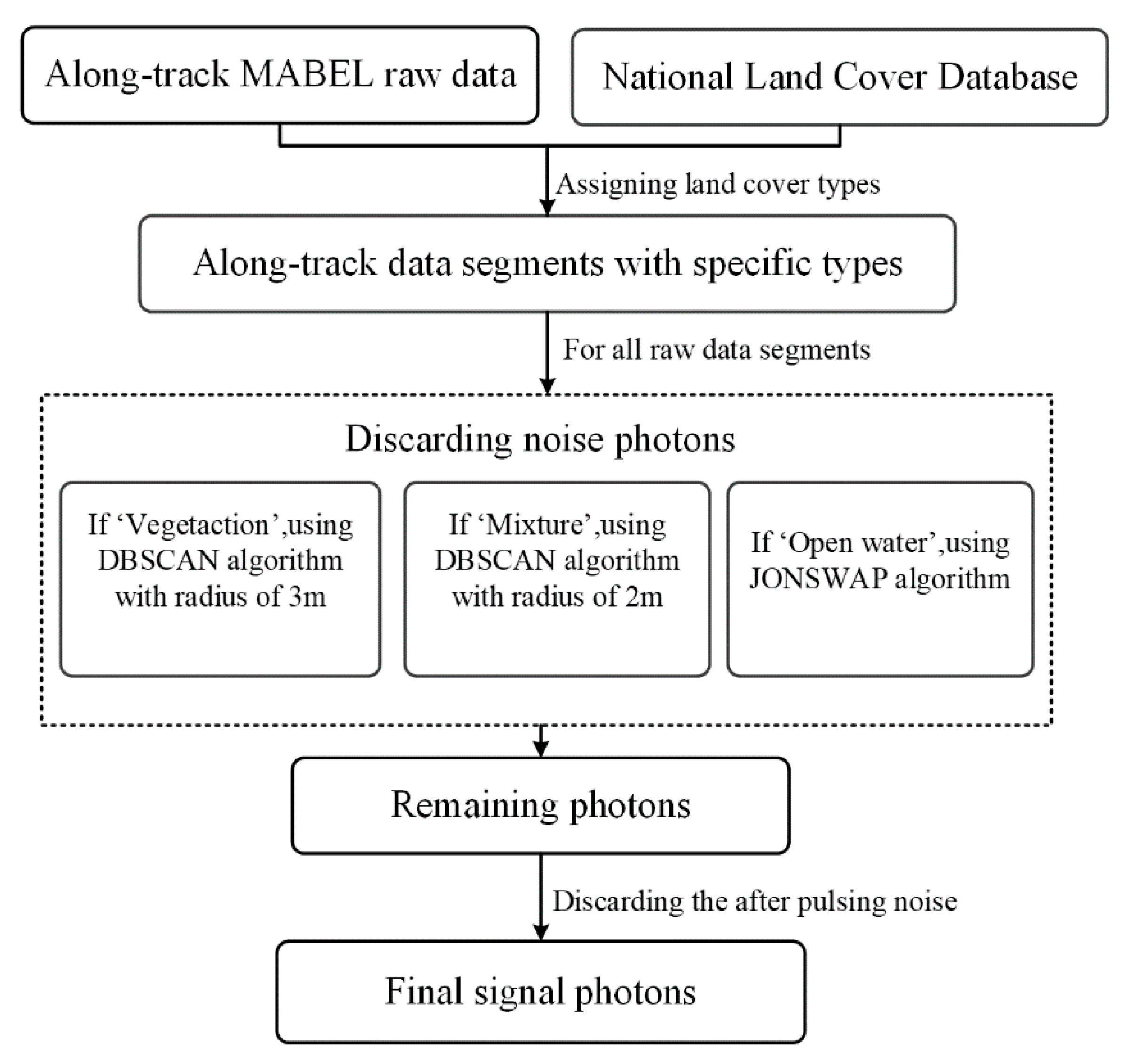
Our proposed method includes three parts for detecting signal photons from the raw data of photon-counting lidar. First, the surface types of the MABEL trajectory with a resolution of 30 m are obtained via matching its geographic coordinates with those in the NLCD datasets (the details are in Section 3.1). Second, for all segments, the raw data are filtered to discard the noise photons via different methods according to their corresponding land cover types. For the ‘vegetation’ and ‘mixture’ types, an improved DBSCAN surface-finding algorithm is proposed and used with different neighborhood radii, and the neighborhood radius and other parameters in this new DBSCAN algorithm are adaptively adjusted according to the spatial statistical characteristics of the inputting photon clouds (the details are described in Section 3.2). For the ‘open water’ type, a JONSWAP spectrum surface-finding algorithm is used (the details are described in Section 3.3). Finally, after the regular process, an extra noise filtering process is undertaken to discard the remaining after-pulsing noise photons to obtain the final signal photons (the details are in Section 3.4). The flow chart of the total process is illustrated in Figure 2. With the NLCD land cover datasets and MABEL raw data, all the steps in this method are automatically processed based on the ArcGIS (to obtain the surface types in Section 3.1) and MATLAB (to detect the signal photons under different surface types in Section 3.2, Section 3.3 and Section 3.4) software environment.

The verification of used methodology is conducted by three steps. First, a comparison of detecting signal photons between our method and the NASA surface finding method is conducted. Referring to various corresponding land covers from the images, the raw data photons, the result photons from the NASA surface finding method, and the result photons from our method are illustrated, and the performance of different methods can be clearly distinguished in this visual comparison. Second, the in-situ data from two nearby NOAA stations are used to evaluate the performance of different methods. The surface parameters are separately calculated using the detecting result photons of our method and the NASA surface finding method and compared with the in-situ surface parameters by comparing the errors between the calculated surface parameters from different methods and the in-situ surface parameters. Third, the average vegetation height in the study area is calculated using the detected signal photons from our method and from the NASA surface finding method. The GFCH dataset that provides forest canopy heights at a global scale is used to evaluate the calculated vegetation height.

3.1. Matching Land Cover Types for MABEL Raw Data

Detailed information on latitude, longitude, elevation, and the time tags of raw data photons can be obtained from the MABEL datasets. All photons are transformed from three-dimensional coordinates (i.e., the geographic coordinates including the latitude, longitude, and elevation based on the WGS84 coordinate frame) to two-dimensional coordinates (i.e., the along-track coordinates including the along-track distance and elevation). The along-track distance starts from the beginning of the MABEL trajectory (in the farthest east of the trajectory and where the distance is zero). It is more convenient to discard the noise photons in a two-dimensional coordinate frame. Each raw photon has a unique index and after the noise filtering process, the remaining signal photons can be represented in three-dimensional geographic coordinates again.

The trajectory of the MABEL datasets is generated by extracting the latitude and longitude coordinates every 5 m along-track. For each trajectory location, the latitude and longitude coordinates are used to match corresponding land cover information from the NLCD 2011 products via the Function “Extract Values to Points” in ArcGIS. Owing to the similar physical properties, we merge some similar land cover types. The ‘shrub/scrub’, ‘cultivated crops’, ‘woody wetlands’, and ‘herbaceous wetlands’ types are combined and named as ‘vegetation’ because all these types belong to vegetation land cover and have very rough profiles. The ‘barren land’ type is merged into ‘mixture of constructed materials and vegetation’ and named ‘mixture’ because both types have relatively flat surfaces and higher reflectance, and the laser photon density of these land cover types is higher compared to vegetation types. The land cover types (‘vegetation’, ‘mixture’, and ‘open water’) are assigned to the MABEL trajectory every 5 m along-track. The MABEL raw photons can be divided into many along-track segments with specific land cover types. In each along-track segment, the raw photons correspond to an identical land cover type. We merge segments whose along-track distance is less than 50 m into its front segment.

3.2. Improved DBSCAN Surface-Finding Algorithm for Land and Vegetation

To extract the signal photons from the raw data corresponding to land types, an improved DBSCAN method is proposed. The DBSCAN algorithm was originally proposed to detect clusters in large noisy spatial databases [30] and was then modified to extract signal photons from the raw data of photon-counting lidar [21]. For every point in a cluster, if the point density in its neighborhood (within a specific radius) exceeds a specific threshold, this point will be classified as a “signal point” based on the criteria of the DBSCAN algorithm. The neighborhood is defined as the Euclidean distance for given points a and b, i.e., dist(a, b). In the DBSCAN algorithm, the clustering parameters R (i.e., the neighborhood radius of a point, defined by dist(a, b) ≤ R) and MinPts (i.e., the minimum number of points within the neighborhood radius) are essential [30]. The surface profiles of vegetation are much more fluctuant than artificial structures. The laser can penetrate the vegetation canopy into the undergrowth vegetation and ground, whereas the laser normally cannot penetrate the surface of artificial structures. Therefore, the signal photon density reflected by vegetation is less than by artificial structures. The neighborhood radius for the ‘vegetation’ type is set to R = 3 m and the neighborhood radius for the ‘mixture’ type is set to R = 2 m. Next, an adaptive algorithm is proposed to determine the MinPts. By inputting the raw data points in the current along-track segment with the ‘vegetation’ or ‘mixture’ type and its corresponding neighborhood radius R, the MinPts can be automatically calculated using the following steps.

(A) The raw data photons along the vertical direction are divided into M segments (M is equal to 50 in this paper) for each MABEL dataset. For each vertical segment, the elevation length h can be expressed as h = R_g/M, where R_g is the range gate (approximately 1500 m for the MABEL). Then, the histogram of photon numbers for each vertical segment can be obtained. If the number of total raw photons in a dataset is N_t, the average photon number in all vertical segments is N_t/M.

(B) According to the histogram, we calculate the number of segments M₂ in which the photon number is smaller than the average photon number N_t/M and calculate the total photon number N₂ in these M₂ segments. In these M₂ vertical segments, most photons are noise photons. Similarly, one can calculate the number of segments M₁ (M₁ = M − M₂) in which the photon number is larger than the average number N_t/M and calculate the total photon number N₁ (N₁ = N_t − N₂) in these M₁ segments. Both signal and noise photons are included in these M₁ vertical segments.

(C) The total along-track distance l in each dataset can be calculated, and the elevation length in each vertical segment is h = R_g/M. For the M₂ segments (corresponding to noise photons), the photon density ρ₂ (count/m²) per unit along-track distance and unit elevation length can be expressed as ρ₂ = N₂/(h·l·M₂). Similarly, for the M₁ segments (corresponding to signal and noise photons), the photon density ρ₂ is expressed as ρ₁ = N₁/(h·l·M₁).

(D) The area S can be calculated as S = π·R² for a given circular zone. Next, for the M² segments, the expected photon number of noise SN₂ within this circular area can be expressed as in Equation (1).

$$S{N}_2={\rho }_2·S=\frac{\pi R^2{N}_2}{hl{M}_2}$$

(1)

Similarly, the expected photon number of signal and noise SN₁ can be expressed as in Equation (2). Then, the expected number of signals can be approximately estimated using SN₁ − SN₂.

$$S{N}_1={\rho }_1·S=\frac{\pi R^2{N}_1}{hl{M}_1}$$

(2)

(E) Given the expected number of noise and signal photons within a neighborhood area, the threshold of photon numbers (the minimum number of points) can be expressed as [14]

$$MinPts=\frac{2S{N}_1-S{N}_2+\ln (M_2)}{\ln \left(\raisebox{1ex}{$2S{N}_1$}\!\left/ \!\raisebox{-1ex}{$S{N}_2$}\right.\right)}$$

(3)

The MinPts can be calculated via the procedure (A) to (E) and the MinPts can be adaptively adjusted by the input raw data. Then, by inputting the neighborhood radius R and the threshold of the minimum number of points in its neighborhood MinPts into the DBSCAN calculator, the signal photons are detected from the raw data photons [30].

3.3. JONSWAP Spectrum Surface-Finding Algorithm for Water Areas

In a previous study, we proposed a method to extract the ocean surface based on the JONSWAP wave spectrum and LM (Levenberg-Marquardt) nonlinear least-squares fitting [7]. This method first constructs an initial sea surface profile according to the wind speed above the sea surface. The wind speed in this area can be estimated from the wind speed data of the MABEL datasets. In each MABEL dataset, the meteorology data provide the wind speed with spatial resolution of approximately 15 m in the east and north at different altitudes. For each MABEL dataset, we can obtain an approximate wind speed by calculating the RSS (Root Sum Square) of the eastward and northward wind. This wind speed is sufficient to be an initial value and the actual surface profile of waters can be automatically adjusted via the LM fitting in the following procedures.

In the JONSWAP spectrum surface-finding algorithm, it is similar to the surface-finding algorithm for land and vegetation, a preliminary data processing procedure is needed to eliminate the gross error that may interfere with the fitting process. The raw data photons are uniformly divided into many segments in the vertical direction, and the photons with a lower point density will be directly discarded. Then, all the remaining photons are used to fit the water surface profile several times. In each fitting process, the 2-sigma criteria are used to discard photons corresponding to larger fitting error. Finally, the remaining data photons are divided into along-track segments with a specified distance (e.g., with an along-track distance of 500 m) and are separately filtered by the LM fitting and 2-sigma discarding. Undergoing these steps, the remaining photons are considered the laser signal photons from water surfaces.

3.4. Discarding the After-Pulsing Noise Photons

Due to the after-pulsing effect of photon-counting detectors, some noise photons will emerge after the laser pulse signal photons. The time tags of after-pulsing noise photons are normally a few tens of nanoseconds (corresponding to approximately 1.5 meters distance) later than the time tags of laser signal photons, and the number of after-pulsing noise photons are approximately one-tenth of the laser signal photons [31]. If the after-pulsing noise photons cannot be discarded, a ranging bias will be introduced (the range between the lidar and target will be overestimated, and the surface elevation of the target will be underestimated). For oceans and other water areas, the JONSWAP spectrum surface-finding algorithm has been proven to be able to eliminate the after-pulsing noise photons [7]. In a coastal area, the elevation of the ground surface is normally higher than the current water level. Therefore, for areas corresponding to the ‘vegetation’ and ‘mixture’ types, the after-pulsing noise photons are discarded as follows. First, for each segment of the ‘vegetation’ and ‘mixture’ types, the nearest water area is searched, and its local water level and RMS wave height are calculated by averaging the elevations of signal photons and calculating their standard deviations. Second, a threshold is equal to the local water level subtracting the tripled RMS wave height (i.e., 3-sigma criteria). We discard the photon in the ‘vegetation’ and ‘mixture’ segments, if the elevation of the photon is lower than the threshold.

4. Results

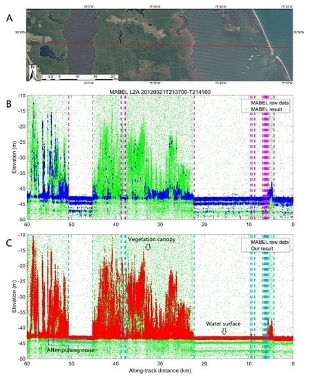
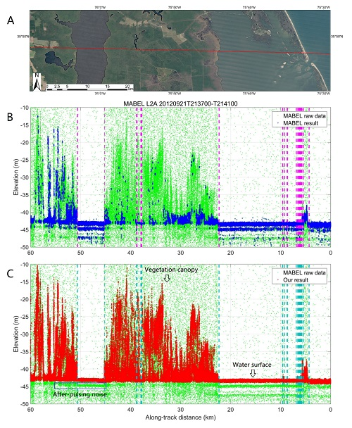
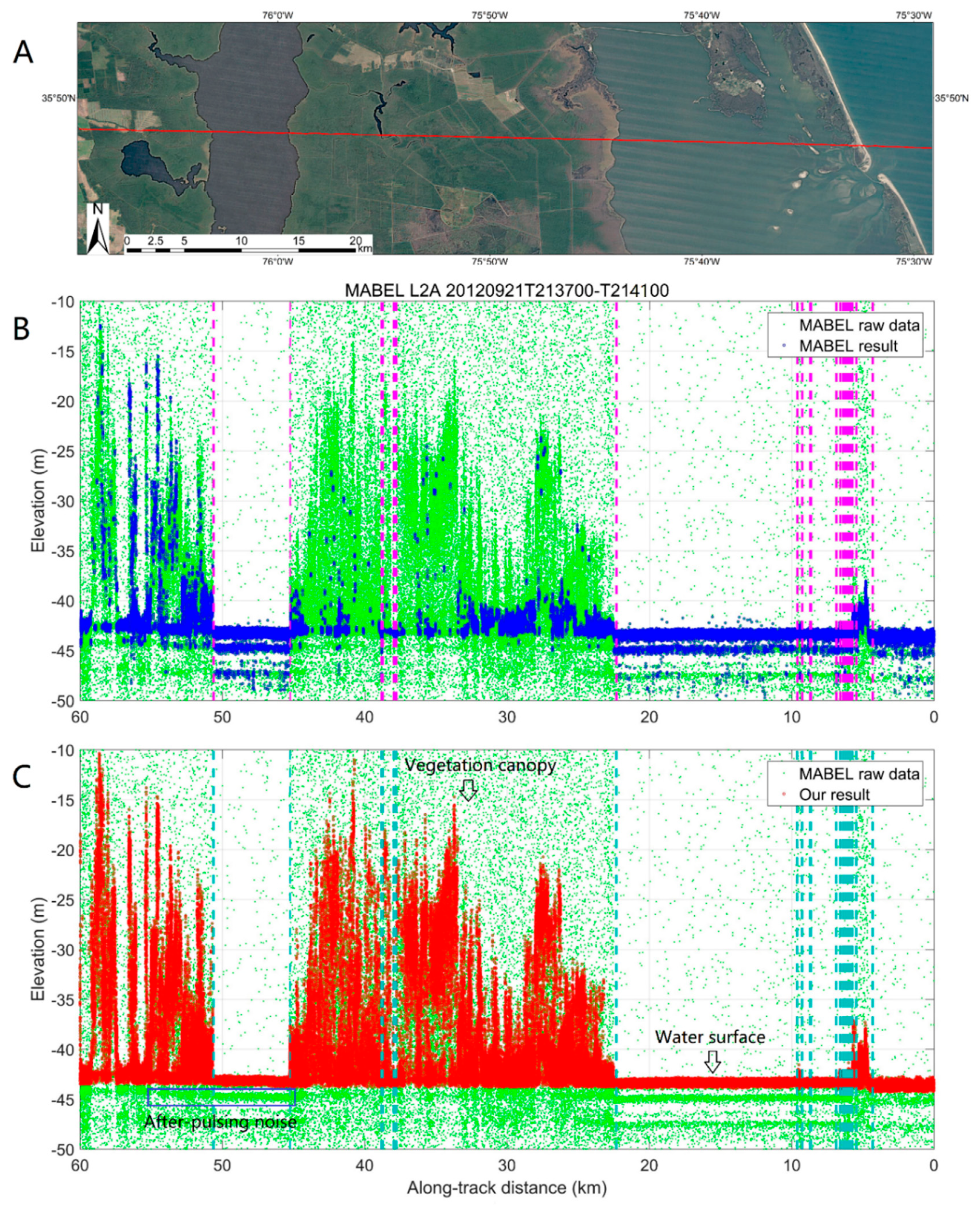
Figure 3 illustrates the MABEL trajectory on Google Maps (using a red line), the captured photons by the MABEL lidar, and the photon results. The top figure in Figure 3 (Figure 3A) shows that on 21/09/2012 from 21:37 to 21:41 GMT (Greenwich Mean Time), when the MABEL lidar flew over Pamlico Sound, it flew over the open water of the Atlantic Ocean, across the Outer Banks of Pamlico Sound (entered into Pamlico Sound), across many small shoals and islands inside Pamlico Sound, over the open water of Pamlico Sound, entered into the land mainly covered by vegetation (flew over a very small, slim lake in the middle of this route), flew over the open water of East Lake, and finally entered the land covered by vegetation. The trajectory was from the east to the west with a path length of 60 km. The middle figure in Figure 3 (Figure 3B) illustrates the along-track raw photons captured by the MABEL lidar and the result of signal photons via the official surface-finding method. The bottom figure (Figure 3C) illustrates the along-track raw photons and the photons resulting from our method. In both Figure 3B,C, the boundaries between different land cover types of the along-track trajectory are illustrated using dashed vertical lines. These boundaries are obtained by matching the geographic coordinates of the MABEL trajectory with the land cover types in the NLCD 2011 products, and these boundaries are in accordance with the land cover image in Figure 3A, which proves that the NLCD 2011 products can provide the land cover types to help detect signal photons from the noisy raw data of a photon-counting lidar.

The raw photons were captured by channel no. 44 at 1064 nm, a near-infrared wavelength. Channel no. 44 has the best quality because it corresponds to a nearly nadir incidence with a better signal-noise ratio. Additionally, the wavelength of 1064 nm is located in the atmospheric window with lower energy loss during the transmission in the atmosphere and has much lower penetration into the water volume compared to the wavelength of 532 nm. The MABEL raw data illustrated using green filled circles are very noisy because they contain both the reflected laser photons (i.e., signal photons) and the noise photons caused by the background, backscatter, and detector noise (including the dark noise and after-pulsing effect). The signal photons of the MABEL result illustrated in Figure 3B (by blue circles) are processed by the official surface-finding algorithm and read from the MABEL dataset ‘ph_class’, which provides the flags for all photons that are classified as “noise”, “buffer”, “low”, “medium”, and “high”. The MABEL results discard most of the noise photons; however, some noise photons remain (some noise photons construct a sublayer surface below the actual surfaces of the water and ground) and some signal photons are discarded, especially for the type of vegetation.

In Figure 3B, the MABEL result failed to detect all the vegetation signal photons because they have a lower point density. The after-pulsing noise photons (in the blue box of the left bottom in Figure 3C) were incorrectly detected because they have higher point density than the vegetation signal photons. The after-pulsing noise photons construct a sublayer surface below the actual water surface and introduce a minus elevation bias to the MSL (mean sea level) or ground surface. In Figure 3C, vegetation signal photons are extracted well and the after-pulsing noise photons below the actual water and ground surfaces are successfully discarded. The signal photons of our result look much better than those of the MABEL result.

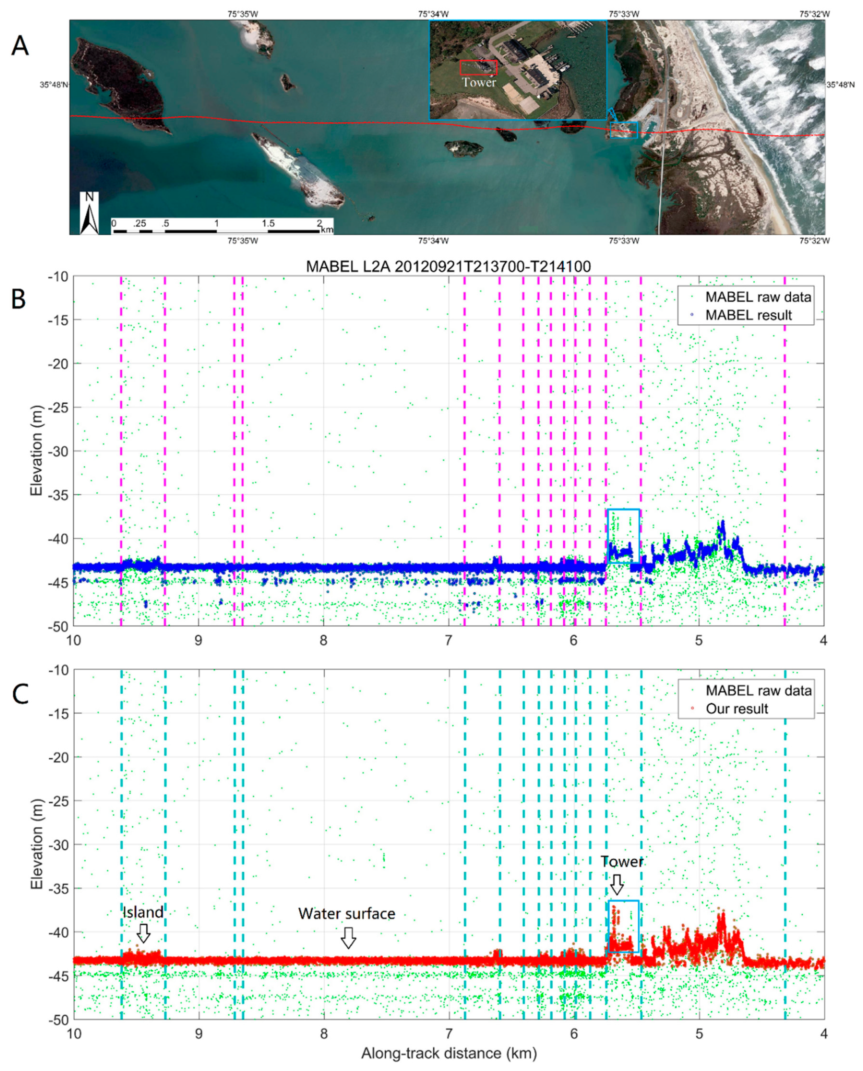
Figure 4 shows the enlarged details of the along-track distance segment from 4 to 10 km in Figure 3. This segment contains multiple land cover types (i.e., ocean, banks, sand, rocks, vegetation, artificial construction, water, and shoals). As mentioned above, all types are considered ‘mixture’ except for the ocean and water surfaces. The boundaries of different land cover types are much denser in this segment, and the NLCD datasets provide acceptable land cover types. The signal photon of the MABEL and our result both successfully extract the surface profile. Some noise photons remain below the water surface in the MABEL result, whereas our result eliminates these after-pulsing noise photons. In the blue box of the top (Figure 4A), middle (Figure 4B), and bottom figures (Figure 4C), a tower was captured by the MABEL lidar. Our result extracts the signal photons reflected by this tower. With our results, the height of this tower can be measured as approximately 6 m above the ground surface.

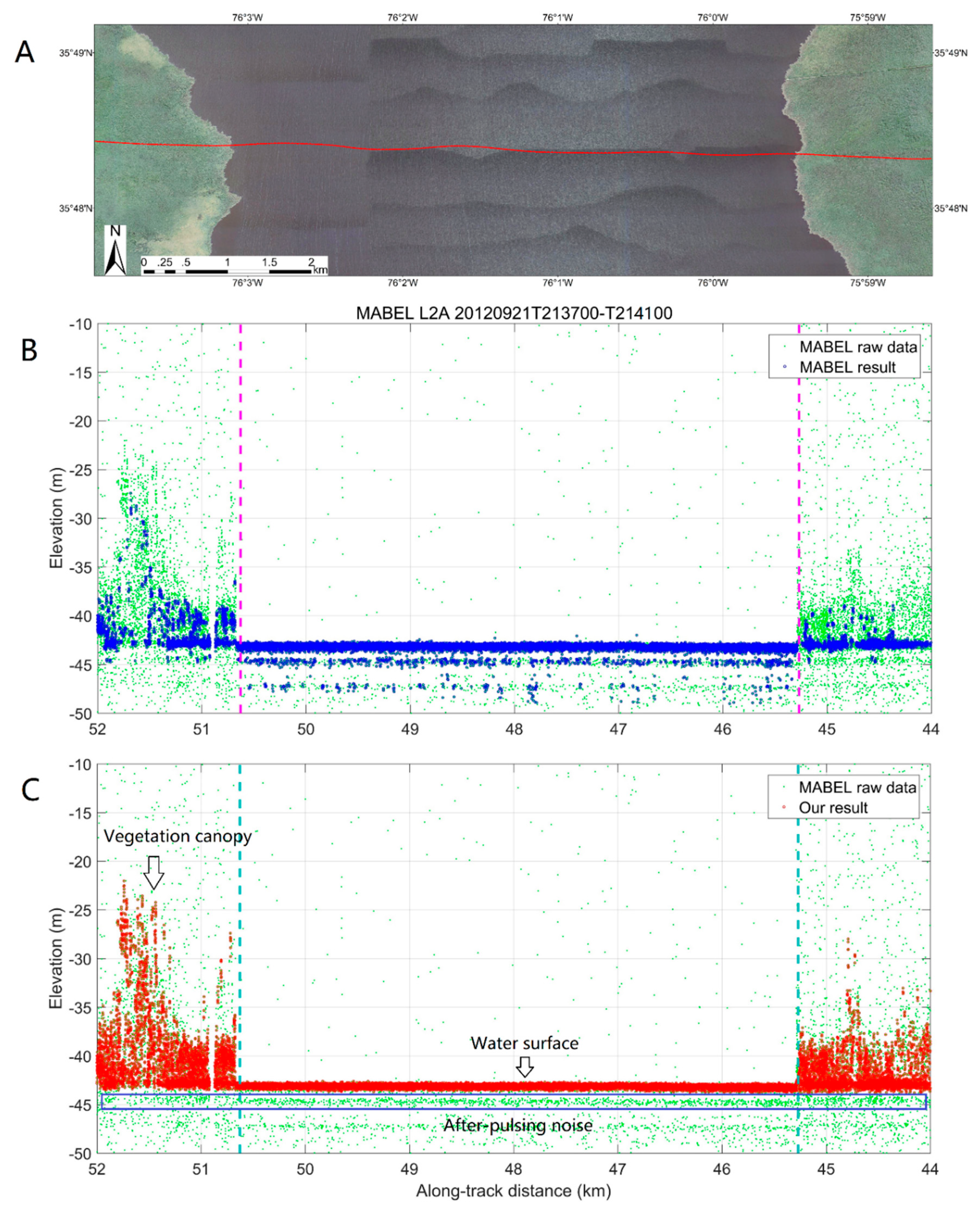
Figure 5 shows the enlarged details of the along-track distance segment from 44 to 52 km in Figure 3. This segment only contains water surface and vegetation. The boundaries between different land cover types of the NLCD datasets precisely divided this along-track segment into open water and vegetation. The signal photon of the MABEL fails to detect the vegetation photons and fails to discard the noise photons below the water surface, whereas our result successfully detects the vegetation photons and eliminated the noise photons below the water surface. From our results, we can estimate the vegetation height from the signal photons. The average height is approximately 5 m near the water boundary, and the maximum vegetation height is approximately 20 m. In Figure 5C, the after-pulsing noise photons are located in the blue box at the bottom. The elevation of after-pulsing noise photons is approximately 1.5 meters below the water and ground surface.

From the overall result figure (Figure 3), most of the land cover types of the along-track signal photons are precisely classified as ‘Vegetation’, ‘Open water’, and ‘Mixture’ in the exception of some very short along-track segments. The surface types are not correctly detected in these very short along-track segments because the segments whose along-track distance is less than 50 m are merged into its front segment. In both the improved DBSCAN algorithm and the JONSWAP algorithm, the raw data with at least 50 m along-track distance is essential to automatically calculate the key parameters (i.e., the minimum number of points within the neighborhood radius (MinPts)) in the DBSCAN algorithm or fit the parameters of the water surface profile (i.e., the amplitudes, angular frequencies, and phases) in the JONSWAP algorithm.

In the enlarged detailed Figure 4, the surface types are classified as ‘Open water’ and ‘Mixture’. In the enlarged detailed Figure 5, the surface types are classified as ‘Open water’ and ‘Vegetation’. Therefore, the proposed method is useful and successful to detect the main surface types in coastal area. Near the land/sea boundary, the tide has a significant effect and can change the surface types from land to sea when the tide is rising and vice versa. Inside the sound, the tide effect is much weaker. The spatial resolution of the surface types from the NLCD products is 30 m, and the spatial accuracy of the surface types is estimated better than 2 pixels (60 m in length) in the exception of the boundary between the land and sea surface.

In Figure 5, for the sea surface, the after-pulsing photons is very obvious and form a sub-layer below the sea surface because a 1064 nm laser nearly cannot penetrate the water volume and the sea surface is relatively flat (compared with the vegetation surface). However, the laser pulse can penetrate the vegetation canopy, so the after-pulsing photons are mixed with the reflected photons by the lower-layer vegetation as well as the ground, which makes the after-pulsing photons not obvious or seems weaker than the sea surface.

5. Discussions

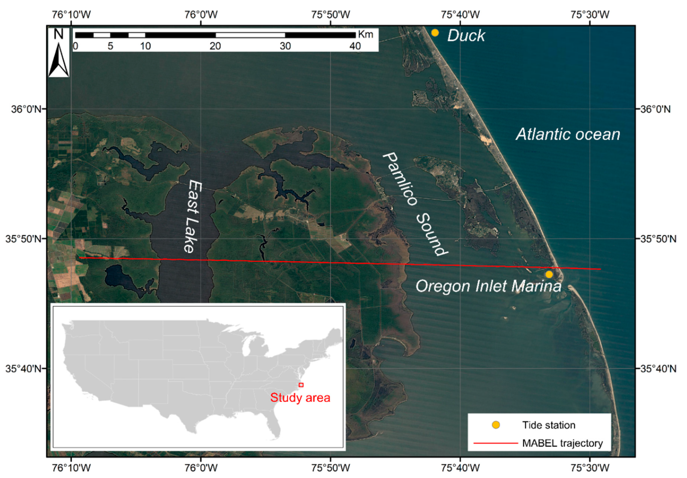
In the coastal areas, the proposed method performed better in extracting the signal photons than the MABEL result. With the detected signal photons, water levels can be estimated by averaging their elevations within water segments. Three segments in the total trajectory corresponded to the water surface, i.e., Segment 1 from 0 to 4.3 km on the ocean surface (in the Atlantic Ocean), Segment 2 from 9.9 to 22.1 km on the water surface (in Pamlico Sound), and Segment 3 from 45.3 to 50.6 km on the water surface (in East Lake). Water levels are −43.62 m (Segment 1 in the Atlantic Ocean), −43.31 m (Segment 2 in Pamlico Sound), and −43.14 m (Segment 2 in East Lake). The water level shows a descending trend from the inner lake and sound to the ocean, in accordance with the water level trend in the study area at that time. The result is because, as shown in Figure 1, the three water regions are linked and according to the water level data of the in-situ stations, the tide was falling when the MABEL lidar flew over this area on 21/09/2012 from 21:37 to 21:41 GMT.

However, if we use the MABEL result to calculate the water level, the water levels will be −43.75 m (in the Atlantic Ocean), −43.46 m (in Pamlico Sound), and −43.37 m (in East lake). The after-pulsing noise photons introduce minus biases to the water level from 13 cm to 23 cm in three segments. At 21:36 GMT, the mean sea levels of Duck Station (corresponding to Segment 1 in the Atlantic Ocean) and the Oregon Inlet Marina Station (corresponding to Segment 2 in Pamlico Sound) were −0.25 m and 0.07 m, respectively. It should be noted that the water levels calculated by the signal photons were on the benchmark of WGS84 ellipsoidal height, whereas the water levels of the in-situ stations were on the benchmark of NAVD88 geoid height. Therefore, we can only make a comparison of the elevation difference between the water levels of the Pamlico Sound and the Atlantic Ocean. The in-situ elevation difference was 0.32 m (the Pamlico Sound had a higher water level than the Atlantic Ocean), and the elevation difference calculated by our result was 0.31 m, whereas the elevation difference calculated by the MABEL result was 0.29 m.

Table 1. Water level comparison between the in-situ data and the calculated result from signal photons.

At 21:36 GMT, 21/09/2012	Atlantic Ocean	Pamlico Sound	East Lake	Difference between Pamlico Sound and Atlantic Ocean	Error Between the Calculated Water Level Difference and in-situ Difference
in-situ water level on NAVD88 geoid height (m)	−0.25 (from Duck Station)	0.07 (from Oregon Inlet Marina Station)	None	0.32	--
Water level calculated by our result on WGS84 ellipsoidal height (m)	−43.62	−43.31	−43.14	0.31	0.01
Water level calculated by MABEL result on WGS84 ellipsoidal height (m)	−43.75	−43.46	−43.37	0.29	0.03

lists a detailed comparison between the in-situ water level and the water levels calculated by our result and MABEL result photons. The error of water level difference of the Atlantic Ocean and Pamlico Sound between our result and the in-situ result is 0.01 m, whereas the water level error between the MABEL result and in-situ data is 0.03 m.

In addition, the RMS wave heights of three segments can be calculated using the signal photons within the water segments and they are 0.32 m (Segment 1 in the Atlantic Ocean), 0.20 m (Segment 2 in Pamlico Sound), and 0.20 m (Segment 3 in East lake). The RMS wave height in the ocean (0.32 m) is larger than the inner water (0.20 m). At 21:36 GMT, the wind at Duck Station was 3.90 m/s at a height of 28.1 feet (approximately 8.58 m) above sea surface, and the wind at Oregon Inlet Marina Station was 3.30 m/s at a height of 21.8 feet (approximately 6.66 m) above the sea surface. According to Businger’s theory [32], these winds can be transferred to 12.5 m above the sea surface as Equation (4).

$$U_{12.5}=U_z\frac{\ln (12.5/z_0)}{\ln (z/z_0)}$$

(4)

U_12.5 is the wind speed at 12.5 m above the sea surface, U_z is the wind speed at the height of z, and z₀ is 0.0023 m when the wind speed is less than 7 m/s. At the height of 12.5 m, the winds at Duck Station (corresponding to Segment 1 in the Atlantic Ocean) and the Oregon Inlet Marina Station (corresponding to Segment 2 in Pamlico Sound) were 3.56 m/s and 4.08 m/s, respectively. The RMS wave height is related to the wind speed above the sea surface and can be expressed as [33]

$$RM{S}_{wh}=0.016U_{12.5}^2$$

(5)

If we substitute the wind speeds of Pamlico Sound and the Atlantic Ocean at the height of 12.5 m into Equation (5), the RMS wave heights were 0.26 m and 0.20 m, respectively, in accordance with those calculated by our result photons (0.32 m and 0.20 m, respectively). However, the RMS wave heights calculated by the MABEL result are much larger (0.70 m and 0.57 m in Pamlico Sound and Atlantic Ocean) and completely different from the result calculated by the in-situ winds.

Table 2. RMS wave height comparison between the in-situ data and the calculated result from signal photons.

At 21:36 GMT, 21/09/2012	Atlantic Ocean	Error Between the Calculated and in-situ Result in Atlantic Ocean	Pamlico Sound	Error Between the Calculated and in-situ Result in Pamlico Sound	East Lake
RMS wave height calculated by the in-situ winds (m)	0.26 (from Duck Station)	--	0.20 (from Oregon Inlet Marina Station)	--	None
RMS wave height calculated by our result photons (m)	0.32	−0.06	0.20	0.00	0.20
RMS wave height calculated by MABEL result photons (m)	0.70	−0.44	0.57	−0.37	0.77

lists a detailed comparison between the RMS wave heights calculated by the in-situ winds, our result photons, and MABEL result photons. In the Atlantic Ocean and Pamlico Sound, the errors of RMS wave heights between our result and the in-situ result are −0.06 m, and 0.00 m, respectively. However, between the MABEL and in-situ results the errors are −0.44 m, and −0.37 m, respectively. With the RMS wave heights, we can further calculate the significant wave height (SWH) as SWH = 4 × RMS wave height.

Moreover, the average vegetation height is calculated using the detected signal photons from our method. The signal photons on the vegetation canopy and the ground are extracted, respectively. The maximum elevation in every 50 m along-track is searched as the canopy elevation in current along-track segment, and the minimum elevation in every 50 m along-track is searched as the ground elevation. The average values of all canopy elevations and all ground elevations are separately calculated. The average canopy height is finally obtained via subtracting the average canopy elevation by the average ground elevation. The GFCH dataset (that is derived from GLAS ICESat data and provides forest canopy heights at a global scale) is used for comparison. The profile of vegetation height is extracted from the raster format GFCH data using the ArcGIS. The mean vegetation height between the East Lake and Pamlico Sound (from 23 km to 45 km within the along-track distance of Figure 3) is also calculated as 15.17 m using the detecting signal photons from our method, which agrees well with the results (15.56 m) from the GFCH dataset. The average vegetation height derived from our results are in accordance with the average vegetation height from the GFCH dataset, whereas the signal photons from MABEL standard result (using the NASA surface finding method) failed to detect the vegetation canopy and cannot obtain the average vegetation height.

With a 30 m spatial resolution, the NLCD datasets provide acceptable land cover types to divide the MABEL along-track raw data into segments with different land cover types. The gross land cover types are verified in this paper, and it is very helpful to detect the signal photons because their clusters are very different for different land cover types due to different surface profiles and reflectance. The MABEL lidar was used as a high-altitude prototype for the ICESat-2 lidar and had similar data photons. Apart from the national scale NLCD datasets, other large-scale land cover products (e.g., GlobeLand30 [34], NLUD-C [35] can also be used to provide the land cover information for the ICESat-2 datasets in the future. With a given land cover type, the signal photons can be effectively detected from the raw data in different areas via this new proposed method. Then, the parameters of different land cover types can be calculated, e.g., the water level, the wave height, the vegetation height, and the tower height.

6. Conclusions

A novel method is proposed to detect the surface profiles of different land cover types from the MABEL raw datasets in coastal areas. First, the surface types of the MABEL trajectory with resolution of 30 m are obtained via matching the geographic coordinates of the MABEL trajectory with the NLCD datasets. The MABEL raw photons can be divided into many along-track segments with specific land cover types. For each along-track segment, the raw photons correspond to an identical land cover type. Second, an improved DBSCAN algorithm with adaptive thresholds is proposed to detect the signal photons from the raw data for the segments of ‘vegetation’ and ‘mixture’ types with different neighborhood radii, whereas an improved JONSWAP wave algorithm is integrated to detect the surface profile of water.

In Pamlico Sound, the result indicates that this new method can effectively detect the signal photons in vegetation, open water, and mixture segments and successfully eliminate the noise photons below the water surface; however, the MABEL result failed to extract the signal photons in vegetation segments and failed to discard the after-pulsing noise photons. With the detected signal photons, the water level, wave height, vegetation height, and tower height are estimated. The water level and RMS wave height calculated by our result achieved a better accordance with the in-situ data. The error of water level difference of the Atlantic Ocean and Pamlico Sound between our result and the in-situ result is 0.01 m, whereas the water level error between the MABEL result and in-situ data is 0.03 m. In the Atlantic Ocean and Pamlico Sound, the errors of RMS wave heights between our result and the in-situ result are −0.06 m, and 0.00 m, respectively. However, the errors of RMS wave heights between the MABEL result and in-situ result is −0.44 m, and −0.37 m, respectively. The mean vegetation height between the East Lake and Pamlico Sound was also calculated as 15.17 m using the detecting signal photons from our method, which agrees well with the results (15.56 m) from the GFCH dataset.

In coastal areas, the land cover types are various and complex; therefore, the distribution and density of signal photons are very different due to differences in surface profiles and reflectance. In this paper, it has been proven that our new proposed method and the NLCD datasets have the potential to provide land cover information for the improvement of the signal photon detection from the MABEL datasets, which is also useful for the ICESat-2 datasets in the future. Even though the land cover types are various and complex in coastal areas, the signal photons can be effectively detected from the raw data via this new proposed method and the detected signal photons can further to obtain the water levels and vegetation heights.