Hyperspectral Image Classification with Multi-Scale Feature Extraction

Abstract

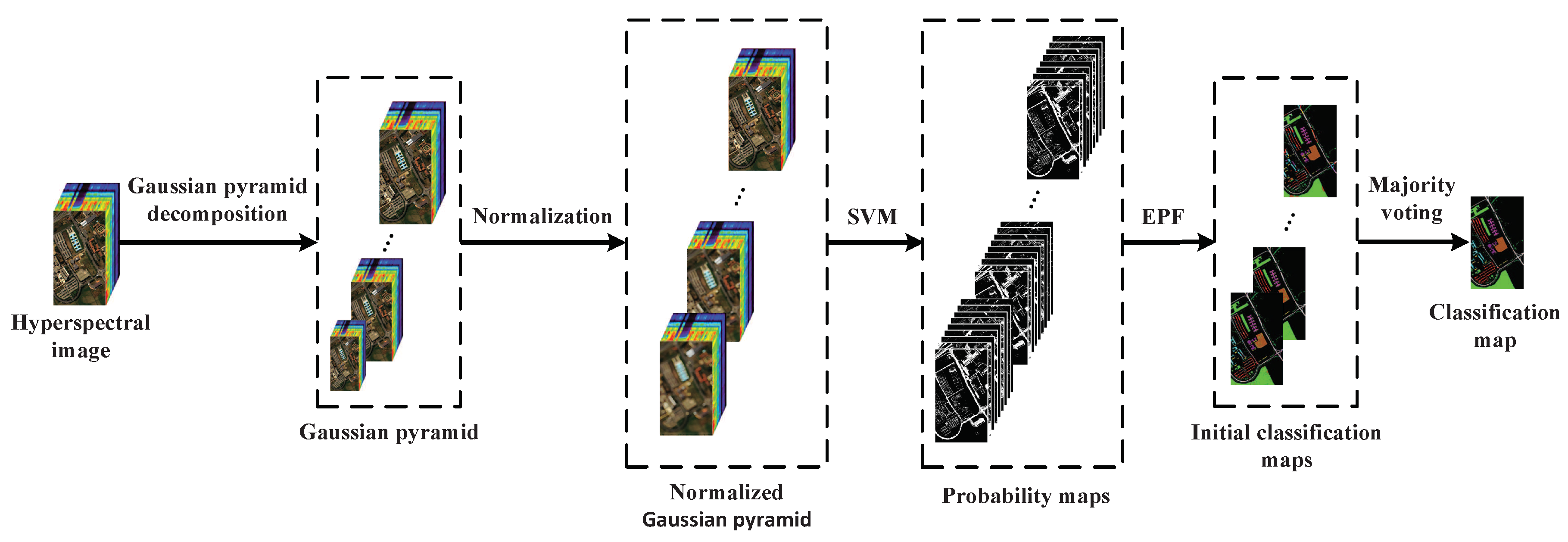
Spectral features cannot effectively reflect the differences among the ground objects and distinguish their boundaries in hyperspectral image (HSI) classification. Multi-scale feature extraction can solve this problem and improve the accuracy of HSI classification. The Gaussian pyramid can effectively decompose HSI into multi-scale structures, and efficiently extract features of different scales by stepwise filtering and downsampling. Therefore, this paper proposed a Gaussian pyramid based multi-scale feature extraction (MSFE) classification method for HSI. First, the HSI is decomposed into several Gaussian pyramids to extract multi-scale features. Second, we construct probability maps in each layer of the Gaussian pyramid and employ edge-preserving filtering (EPF) algorithms to further optimize the details. Finally, the final classification map is acquired by a majority voting method. Compared with other spectral-spatial classification methods, the proposed method can not only extract the characteristics of different scales, but also can better preserve detailed structures and the edge regions of the image. Experiments performed on three real hyperspectral datasets show that the proposed method can achieve competitive classification accuracy.

1. Introduction

Hyperspectral remote sensing technology can acquire spectral images of continuous bands to achieve accurate identification of surface objects. Therefore, it has been widely used in many applications, such as environmental monitoring [1,2,3], national defense [4], and precision agriculture [5,6]. Moreover, a very important application of hyperspectral remote sensing is the classification of hyperspectral images (HSIs) [7,8,9,10,11,12].

Numerous techniques have been developed for HSI classification. As one of the typical classifiers, the support vector machine (SVM) [13,14,15] has been proven to be effective for hyperspectral imagery. By learning an optimal decision hyperplane, SVM can effectively separate training samples in the high dimensional feature space [16]. In addition, other HSI classification methods have been proposed, such as multinomial logistic regression (MLR) [17,18,19], neural networks [20,21,22], kernel-based techniques [23,24], and active learning [25,26]. A detailed discussion about advanced spectral classifiers and their performance can be found in [27]. In addition, sparse representation (SR) [28,29] has been proven to be a useful tool for HSI classification providing a compact representation in a dictionary as a combination of linear atoms. The sparse representation has been extended to HSI classification in [30,31].

However, HSIs not only contain rich ground image information, but also have abundant spectral information. These methods only consider spectral information, ignoring the spatial correlation of neighboring pixels. Therefore, various spatial-spectral classification methods have been developed [32,33,34]. For example, Kang et al. proposed a spectral-spatial classification method based on edge-preserving filtering (EPF) [35]. EPF has been a research hotspot in image processing and computer vision in recent years, which not only has the function of image smoothing, but also can import spatial structure information into the input image. Moreover, a novel spectral-spatial classification for HSIs is proposed [36], which attempts to utilize the within-class similarity between the training and test samples, while reducing the between-class interference. A composite kernel approach can also effectively combine the spectral-spatial information of each pixel [37,38]. Considering that different scales regions contain complementary but interconnected information for classification, Fang et al. proposed a multiscale adaptive sparse representation (MASR) model [39]. The MASR makes full use of multiple scales spatial information through an adaptive sparse strategy. In other works, effective feature extraction algorithms [40,41] and multifeature fusion [42,43] techniques have been developed in which the spectral-spatial characteristics of different materials in the image scene are more effectively represented. Peng et al. proposed a region kernel to measure the region-to-region distance similarity for HSI classification [44]. The region kernel is designed to be a linear combination of multiscale box kernels, which can handle the HSI regions with arbitrary shape and size. These methods consider the spatial context information of the pixel and surrounding pixels while using the spectral information of the ground object for classification. Therefore, they can effectively reduce the influence of the phenomenon of the same object with different spectrum and different objects with the same spectrum on the classification accuracy. Meanwhile, the classification accuracy can also be greatly improved.

Based on the above works, many researchers have made further explorations on the extraction of spatial-spectral features. Therefore, different kinds of multi-scale feature extraction methods were proposed to improve the accuracy of HSIs classification. For instance, Zhao et al. proposed a deep learning framework for extracting deep learning features using multi-scale convolutional auto-encoder [45]. In addition, morphological and neurological methods were used to extract the spectral–spatial features to classify the hyperspectral images of urban areas [46]. By further studying the multi-scale feature extraction method [47,48], we found that the spectral features between pairs of pixels exhibit different spectral separability in multi-scale structures. Therefore, this paper proposed a multi-scale feature extraction (MSFE) method for HSI classification. In the proposed method, the Gaussian pyramid decomposition is employed to decompose the original HSI into a multi-scale structure. Then, we use the EPF method for image smoothing in each layer of the Gaussian pyramid. Finally, in order to get better classification results, we use the majority voting method to determine the label of the pixel. Experiments on three well-known HSI datasets demonstrate that the proposed method can obtained high classification accuracy.

The remainder of this paper is structured as follows: First, Section 2 introduces the proposed MSFE methods. Experimental results and analysis are reported in Section 3. Finally, conclusions are discussed in Section 4.

2. Proposed MSFE for HSI Classification

2.1. Proposed Classification Framework

For the purpose of improving the separability of the hyperspectral features of different features, we choose Gaussian pyramid for multi-scale feature extraction. Figure 1 shows the schematic diagram of the proposed classification method, which consists of the following major steps: First, the HSI is decomposed into several Gaussian pyramids to extract multi-scale features. Second, we construct and optimize probability maps in each layer of the Gaussian pyramid. Finally, the final classification map is acquired by the majority voting method.

2.2. Feature Extraction Based on Gaussian Pyramid Decomposition

Gaussian pyramid decomposition [49] is a series of low-pass sampling filters for images. The filtered image has a lower resolution and sampling density than the previous image. The Gaussian pyramids can be used to scale images on a single scale for multi-scale analysis of images. In this paper, the Gaussian pyramid decomposition operation is performed on the original HSI. Let the original image, ${\mathbf{O}}_1$, be used as the first layer of the Gaussian pyramid. Then, ${\mathbf{O}}_1$ is convolved with a Gaussian kernel and downsampled (or even delete rows and columns). The resulting image, ${\mathbf{O}}_2$, is generated after ${\mathbf{O}}_1$ is low-pass filtered and downsampled. Specifically, in the down-sampling process, when the pixels in rows and columns of an image are removed, the gray value of the pixel on the spatial position (m,n) in the l-th layer of the image can be calculated by an iterative algorithm as follows:

$${\mathbf{O}}_1\left(m,n\right)=\sum _{u=-c}^c\sum _{v=-c}^{c}F\left(u,v\right)\ast {\mathbf{O}}_{l-1}\left(2m-1-u,2n-1-v\right)$$

(1)

where * is the convolution operation. $l\in \left\{2,3,\cdots ,L\right\}$ and L is the total number of layers in the Gaussian pyramid. The F(u, v) is a $\left(2c+1\right)\times \left(2c+1\right)$ Gaussian window that can be defined as:

$$F\left(u,v\right)=\frac{1}{2\pi {\tau }^2}{e}^{-\left(u^2+v^2\right)/2{\tau }^2}$$

(2)

where $\tau$ is the variance of the Gaussian filter. The Gaussian pyramid is composed of a series of images $\left\{{\mathbf{O}}_1,{\mathbf{O}}_2,\cdots ,{\mathbf{O}}_L\right\}$ which are generated from the above convolution and down-sampling operations.

Except for the first layer, the nearest neighbor interpolation method is used to normalize each layer of the gaussian pyramid until the space size becomes the same as the first layer. In this way, multi-scale features will be combined for the subsequent processing step. The normalized Gaussian pyramid, $\mathbf{E}$, can be calculated as follows:

$$\mathbf{E}=NGP(\mathbf{O},L,\tau )$$

(3)

where L (which is the total number of the layers in the Gaussian pyramid) is determined by the size of the HSI, and $\mathbf{O}$ represents the input data.

2.3. Probability Maps Construction and Optimization

The probability maps are constructed and optimized in each layer of the normalized Gaussian pyramid. The initial classification result, C, can be obtained by SVM classifiers in each layer of the normalized Gaussian pyramid. The initial classification result, C, can be expressed in the form of a probability map, in which each pixel i is assigned to a label $C_i$. The initial probability map in the lth layer can be represented as probability maps i.e., $\mathbf{P}=({\mathbf{P}}_1,{\mathbf{P}}_2,\cdots ,{\mathbf{P}}_c)$, where ${\mathbf{P}}_{i,c}\in [0,1]$ is the probability that a pixel, i, belongs to the cth class. Then, the probability ${\mathbf{P}}_{i,c}$ is denoted as

$${\mathbf{P}}_{i,c}=\left\{{}_{0otherwise}^{1if{C}_i=c}\right.$$

(4)

The pixel-wise classification based on SVM does not consider the spatial information of HSIs. All probability values are either zero or one. The initial probability maps contain many noisy elements, and they are not aligned with real object boundaries. Therefore, we employ the EPF to optimize the initial probability maps. Specifically, the optimized probabilities can be denoted as a weighted average of their neighborhood probabilities

$${\tilde{\mathbf{P}}}_{i,c}=\sum _m{W}_{i,m}\left(M\right){\mathbf{P}}_{m,c}$$

(5)

where i and m represent the ith and mth pixels, respectively. The filtering weight, W, is chosen to preserves edges of a specified guidance image, M.

Therefore, the filtering weight, W, and the guidance image, M, can be solved by the following two steps. First, the filtering weight is obtained by the guided filtering method in EPF [35]. The guided filter is a filtering algorithm based on a local linear model. Assuming that M is the guidance image, $\mathbf{Q}$ is the filtering output, and s is the filtering size, then, in a local window, w, with a size of $\left(2\mathrm{s}+1\right)\times \left(2\mathrm{s}+1\right)$, $\mathbf{Q}$ can always be expressed as a linear transformation of M as follows:

$${\mathbf{Q}}_i=a_m{M}_i+b_m,\forall i\in w_m$$

(6)

where the $a_m$ and $b_m$ are the linear transformation parameters. Take the derivative of both sides of this equation and we get $\nabla \mathbf{Q}\approx a\nabla M$; that is, when M has an edge structure at a certain position, the same position of $\mathbf{Q}$ will lead to the similar edge structure. To determine the coefficients $(a_m,b_m)$, the energy function can be denoted as follows:

$$E\left(a_m,b_m\right)=\sum _{i\in w_m}\left({\left(a_m{M}_i+b_m-{\mathbf{O}}_i\right)}^2+\zeta a_m^2\right)$$

(7)

where $\zeta$ (which is a regularization parameter) determines the degree of the blurring for the guided filter. By solving the energy function, the final filtering result is obtained by combining the edge information of M with the pixel information of the input image $\mathbf{O}$. In addition, the output image and guide image must satisfy the local linear model. $\mathbf{Q}$ needs to be close to the input image, $\mathbf{O}$. The local linear model in Equation (6) can also be expressed as a weighted sum form (5). The filtering weight $W_{i,m}\left(M\right)$ for the guided filter can be represented as follows:

$$W_{i,m}\left(M\right)=\frac{1}{{\left|\omega \right|}^2}\sum _{k\in {\omega }_{i,}k\in {\omega }_m}\left(1+\frac{\left(M_i-{\mu }_k\right)\left(M_m-{\mu }_k\right)}{{\sigma }_k^2+\zeta }\right)$$

(8)

where ${\omega }_i$ and ${\omega }_m$ are local windows with pixel i and pixel m, respectively. ${\mu }_k$ and ${\sigma }_a$ represent the mean and variance of the guided image, M, in ${\omega }_k$. $\left|\omega \right|$ represents the number of pixels in ${\omega }_k$. If $M_i$ and $M_m$ are on the same side of the edge, the sign of $\left(M_i-{\mu }_k\right)\left(M_m-{\mu }_k\right)$ in (8) is positive. Conversely, if $M_i$ and $M_m$ are on different sides, the sign of the term is negative. In other words, the filtering weight on the same side of the edge is higher; otherwise, it is lower. Based on this principle, the probability values corresponding to the pixels on the same side of the edge in the guidance image are usually similar to the filtering output.

Second, we employ the gray-scale guidance image as the guidance image for EPF. The original HSI is firstly decomposed by principal component analysis (PCA) [50]. The first principal component with the largest variance is used as the guidance image of the EPF. This can give an optimal representation of the HSI in the mean square and retain as much significant information as possible.

After filtering the probability maps, the label of pixel i can be simply selected in a probability maximization manner. The purpose is to use the SVM supervised classifier to convert the probability map into the initial classification result map. Therefore, each layer of the Gaussian pyramid obtains an initial classification map. Finally, the final classification map is obtained by the majority voting method as follows:

$${\mathbf{C}}_i=arg\underset{t}{max}{c}_{i,t}$$

(9)

where $c_{i,t}$ means that pixel i is marked with label c for t times in each initial classification map of the Gaussian pyramids.

3. Experimental Results

3.1. Data Set

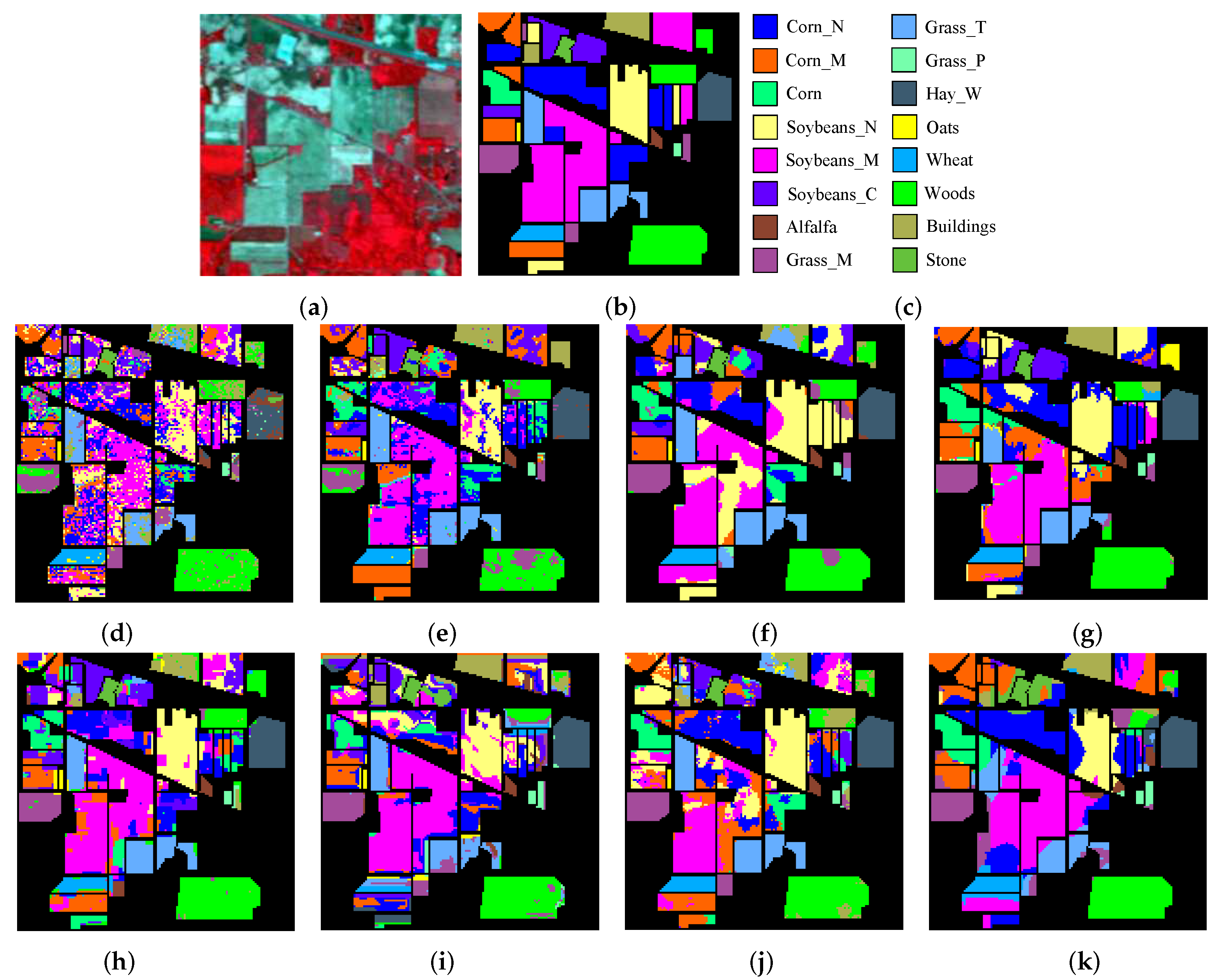
(1) The Indian Pines image was captured in 1992, by the Airborne Visible/Infrared Imaging Spectrometer (AVIRIS) sensor. It captures the agricultural Indian Pine test site of North-western Indiana. The size of the image is $145\times 145\times 220$. The spatial resolution of this image is 20 m per pixel, and the spectral coverage ranges from 0.4 to 2.5 $\mathsf{\mu }$m. In the experiment, 20 water absorption bands (nos. 104–108, 150–163, and 220) were discarded. Figure 2a–c shows the false-color composite and the corresponding reference data of the Indian Pines image.

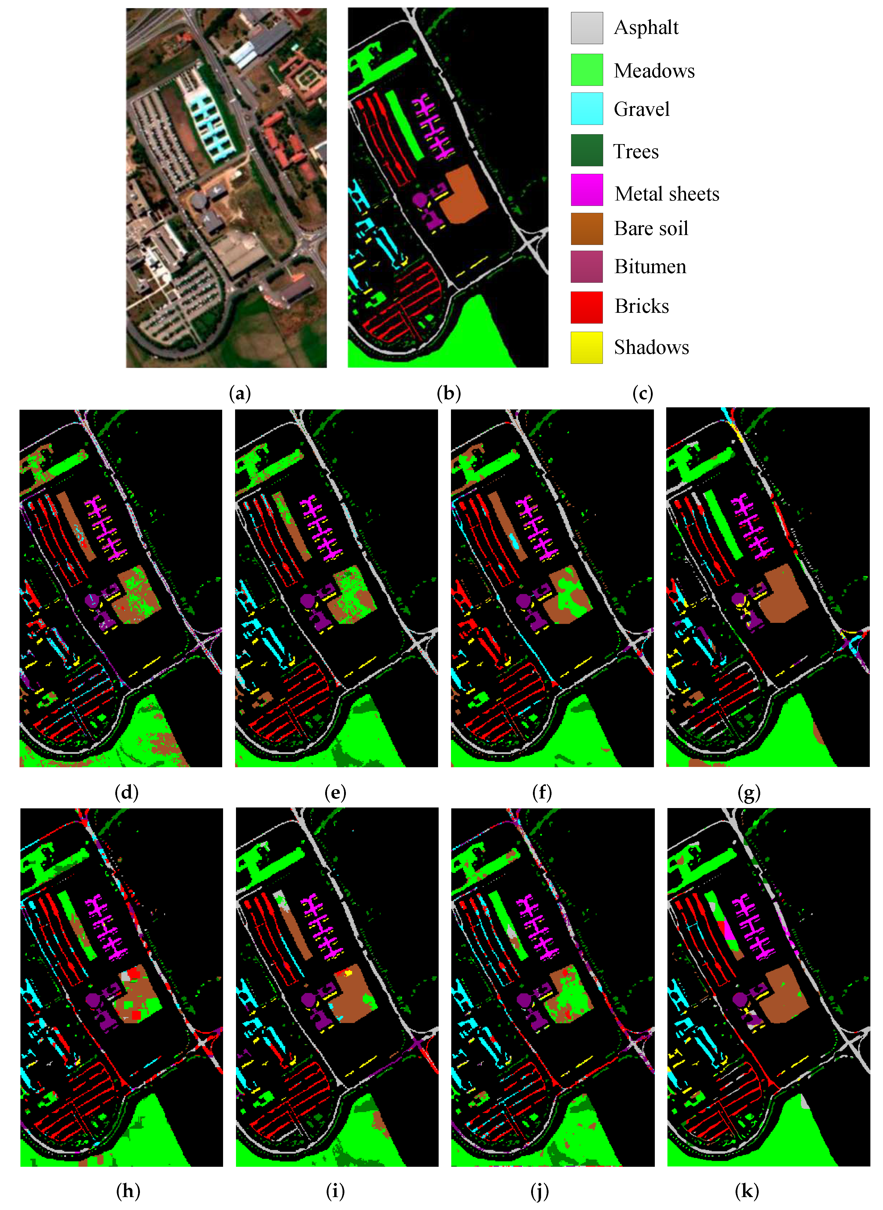
(2) The University of Pavia image which was captured over an urban area surrounding the University of Pavia, Italy. This data set was recorded by Reflective Optics System Imaging Spectrometer (ROSIS). The size of the image is $610\times 340\times 115$. The spatial resolution of this image is 1.3 m per pixel, and the spectral coverage is ranging from 0.43 to 0.86 $\mathsf{\mu }$m. In the experiment, 12 water absorption bands were discarded. Figure 3a–c demonstrates the false-color composite of the University of Pavia image and the corresponding reference data.

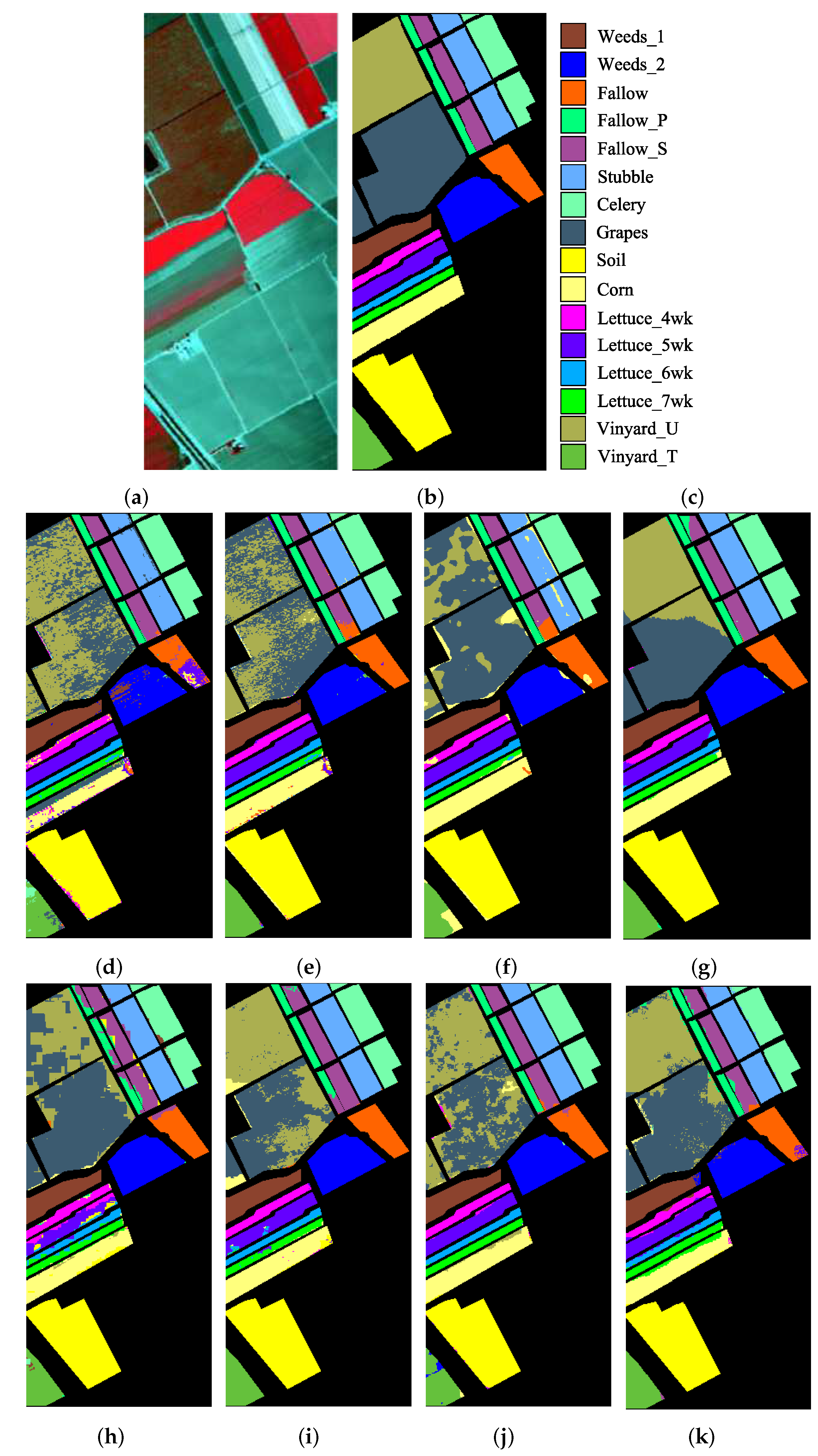
(3) The Salinas image was also captured by the AVIRIS sensor over Salinas Valley, California. The size of the image is $512\times 217\times 224$. The geometric resolution of this image is 3.7 m per pixel. Similar to the Indian Pines image, 20 water absorption bands (nos. 108–112, 154–167, and 224) were discarded. The false-color composite and the corresponding reference data of the Salinas image are shown in Figure 4a–c.

3.2. Comparisons with Other Approaches

In the experiments, three quality indexes, i.e., overall accuracy (OA), average accuracy (AA), and Kappa coefficient are used to impersonally evaluate classification results. In this section, the proposed MSFE method is compared with the SVM [13], extended morphological profiles (EMP) [51], EPF [35], image fusion and recursive filtering (IFRF) [34], joint sparse representation (JSR) [30], superpixel-based classification via multiple kernels (SCMK) [52], and MASR [39] methods. The implementation of other comparisons methods is through the default parameters given by the authors. Here, the SVM algorithm utilizes the library for support vector machines with a Gaussian kernels. The EMP exploits the spatial information, which can improve the estimation. The EPF not only has the function of image smoothing, but also can incorporate spatial structure information into the input image. The IFRF method is to divide the hyperspectral image into multiple subsets of adjacent hyperspectral bands and then, by averaging, the bands in each subset. Finally, the fusion band is processed using transform domain recursive filtering to obtain the resulting features for classification. The JSR utilizes a joint sparsity model in which hyperspectral pixels are concentrated near test pixels. The SCMK effectively utilize the spectral information and spatial structure of superpixels through multiple kernels. The MASR makes effective use of multi-scale spatial information based on adaptive sparse strategy. The experiments of all methods are repeated ten times and samples were randomly selected in each experiments for the purpose of obtaining the average accuracy and standard deviation. The details of the number of training samples and test samples are displayed in

Table 1. Classification Accuracy (in percentage) Obtained by the SVM, EMP, EPF, IFRF, JSR, SCMK, MASR, and MSFE Methods. Class-specific accuracy values are in percentage.

The number of training samples for each class is six for the Indian Pines data set (in %).
Class	Training/Test	SVM	EMP	EPF	IFRF	JSR	SCMK	MASR	MSFE
Alfalfa	6/40	23.33(7.93)	92.50(5.00)	59.25(15.51)	50.89(31.41)	99.25(1.68)	95.5(3.87)	98.00(2.58)	69.40(28.66)
Corn_N	6/1422	45.91(8.96)	40.62(10.34)	66.58(18.03)	65.66(14.58)	47.69(12.44)	41.74(8.53)	48.69(10.87)	75.03(20.58)
Corn_M	6/824	31.66(8.06)	55.97(21.01)	60.84(23.18)	56.01(11.74)	57.32(9.09)	45.22(9.25)	57.68(13.88)	62.80(26.62)
Corn	6/231	21.44(6.68)	59.05(10.94)	44.80(29.70)	50.34(11.66)	83.33(7.61)	73.03(17.64)	86.06(16.50)	76.55(14.12)
Grass_M	6/477	56.15(12.69)	68.43(17.50)	75.92(17.32)	73.55(11.49)	84.74(6.24)	66.08(13.02)	77.74(19.79)	62.46(32.18)
Grass_T	6/724	76.79(4.03)	88.51(11.48)	90.04(6.15)	86.36(6.77)	85.87(4.32)	73.73(11.82)	94.53(3.98)	63.39(3.98)
Grass_p	6/22	24.85(11.15)	93.64(2.49)	56.14(35.63)	34.19(11.70)	98.18(3.83)	96.36(10.00)	100.0(0.00)	47.42(29.74)
Hay_W	6/472	95.93(2.18)	91.57(8.14)	99.38(1.22)	100.0(0.00)	95.95(3.89)	96.61(3.93)	91.10(9.60)	71.26(26.60)
Oats	6/14	11.91(8.56)	97.14(6.39)	39.45(24.67)	29.58(23.10)	95.00(11.69)	100.0(0.00)	100.0(0.00)	53.30(30.07)
Soybean_N	6/966	39.90(6.59)	61.68(12.95)	46.95(13.10)	61.62(13.70)	74.76(15.74)	54.80(9.23)	77.04(10.62)	66.78(19.53)
Soybean_M	6/2449	59.89(6.49)	48.33(11.74)	70.41(7.26)	85.45(7.57)	55.49(12.92)	52.29(10.97)	60.71(12.64)	70.46(29.13)
Soybean_C	6/587	23.80(9.34)	40.44(6.75)	38.56(9.40)	56.44(8.14)	59.25(9.20)	37.63(7.56)	61.07(8.75)	75.45(20.65)
Wheat	6/199	80.40(7.22)	97.89(0.22)	96.76(5.59)	66.18(18.77)	96.23(3.52)	76.78(13.11)	99.65(0.67)	58.16(28.75)
Woods	6/1259	86.90(8.86)	72.10(9.99)	91.37(9.09)	96.80(3.07)	90.75(5.91)	75.14(7.88)	82.12(10.44)	77.49(13.71)
Buildings	6/380	27.74(8.03)	78.79(1.24)	72.41(22.41)	80.60(10.73)	57.79(10.62)	80.13(14.29)	61.24(11.13)	54.00(34.78)
Stone	6/87	84.60(24.08)	88.97(5.05)	78.55(12.81)	90.13(20.06)	94.71(6.06)	86.67(11.34)	99.89(0.36)	66.06(25.63)
OA		48.63(3.46)	61.42(4.11)	63.76(2.75)	68.97(5.52)	68.57(2.30)	59.32(3.12)	69.62(3.68)	73.92(3.80)
AA		49.45(2.86)	74.64(2.86)	68.04(3.60)	67.56(3.37)	79.77(1.15)	71.98(2.20)	80.97(2.67)	64.92(4.42)
Kappa		42.58(3.76)	56.83(4.51)	59.17(3.09)	65.27(6.19)	64.68(2.36)	54.55(3.19)	65.77(3.96)	70.77(4.12)

,

Table 2. Classification Accuracy (in percentage) Obtained by the SVM, EMP, EPF, IFRF, JSR, SCMK, MASR, and MSFE Methods. Class-specific accuracy values are in percentage.

The number of training samples for each class is six for the University of Pavia data set (in %).
Class	Training/Test	SVM	EMP	EPF	IFRF	JSR	SCMK	MASR	MSFE
Asphalt	6/6625	91.85(10.00)	80.53(11.37)	93.81(5.79)	57.79(14.95)	24.47(9.67)	88.62(5.22)	29.65(6.68)	77.31(10.89)
Meadows	6/18,643	79.18(5.26)	53.07(13.71)	84.52(6.61)	92.02(4.66)	69.92(14.54)	69.39(13.34)	62.46(11.91)	95.78(1.79)
Gravel	6/2093	31.38(8.19)	72.37(17.43)	42.16(15.92)	44.79(14.98)	72.17(8.88)	78.18(8.48)	79.53(10.11)	81.09(8.14)
Trees	6/3058	56.84(14.68)	94.68(3.74)	50.74(18.57)	60.89(19.07)	76.68(11.15)	84.37(4.29)	90.08(6.48)	58.61(12.57)
Metal sheets	6/1339	91.01(5.27)	95.13(13.93)	92.21(7.78)	99.76(0.47)	95.15(4.77)	96.43(8.18)	100.0(0.00)	67.57(9.17)
Bare soil	6/5023	26.71(5.81)	60.09(19.12)	33.23(10.34)	66.26(16.07)	63.30(11.12)	77.40(12.52)	59.70(19.54)	82.04(9.16)
Bitumen	6/1324	33.50(7.14)	98.36(0.71)	44.85(17.18)	48.62(11.21)	88.86(6.26)	86.47(10.25)	98.16(1.26)	72.35(17.40)
Bricks	6/3676	65.44(12.08)	77.57(17.97)	65.39(11.62)	47.36(7.71)	78.52(11.66)	80.52(7.60)	62.60(13.19)	76.16(18.71)
Shadows	6/941	99.75(0.35)	99.35(1.64)	97.85(2.12)	48.86(19.09)	19.01(7.65)	90.38(9.88)	35.99(9.45)	82.77(12.59)
OA		55.69(5.57)	67.93(8.52)	61.32(7.60)	66.82(6.79)	63.69(4.99)	77.36(4.80)	61.57(5.44)	81.35(3.31)
AA		63.96(4.14)	81.24(5.15)	67.20(4.07)	62.93(5.60)	65.34(1.20)	83.75(3.46)	68.69(3.17)	77.07(3.18)
kappa		46.71(5.54)	60.60(8.05)	52.96(8.03)	58.39(7.81)	54.60(4.90)	71.45(5.70)	52.39(5.78)	76.06(3.89)

and

Table 3. Classification Accuracy (in percentage) Obtained by the SVM, EMP, EPF, IFRF, JSR, SCMK, MASR, and MSFE Methods. Class-specific accuracy values are in percentage.

The number of training samples for each class is six for the Salinas data set (in %).
Class	Training/Test	SVM	EMP	EPF	IFRF	JSR	SCMK	MASR	MSFE
Weeds_1	6/2003	97.24(3.88)	98.44(2.99)	99.61(1.23)	77.95(8.74)	99.99(0.05)	97.99(5.49)	100.0(0.00)	90.80(6.42)
Weeds_2	6/3720	98.60(0.79)	96.76(4.01)	99.91(0.17)	91.55(11.95)	99.78(0.21)	97.87(2,85)	99.57(0.35)	96.30(2.78)
Fallow	6/1970	79.69(14.43)	92.05(8.70)	88.03(7.09)	99.70(0.29)	96.05(4.47)	100.0(0.00)	90.97(12.44)	93.03(4.58)
Fallow_P	6/1388	97.16(0.48)	99.03(0.83)	97.44(0.64)	78.13(0.72)	70.10(9.96)	94.01(7.06)	98.70(0.75)	68.03(10.82)
Fallow_S	6/2672	97.00(3.14)	93.94(4.45)	99.57(0.52)	97.51(3.40)	79.37(8.12)	97.34(1.17)	98.95(0.99)	95.63(3.10)
Stubble	6/3953	99.96(0.07)	93.70(4.61)	99.97(0.04)	100.0(0.00)	99.26(0.69)	99.75(0.01)	99.95(0.08)	97.42(1.77)
Celery	6/3573	95.11(2.48)	97.37(5.65)	97.54(2.15)	82.68(7.58)	95.71(4.35)	99.64(0.78)	99.74(0.80)	98.78(1.68)
Graps	6/11,265	65.11(8.55)	65.39(12.89)	74.75(10.42)	93.70(8.86)	59.06(16.80)	67.23(8.85)	63.24(3.82)	93.47(3.00)
Soil	6/6197	98.15(1.27)	97.67(1.91)	99.31(0.22)	99.62(0.43)	98.48(4.60)	99.93(0.16)	99.49(0.43)	99.59(0.14)
Corn	6/3272	67.83(15.65)	90.97(4.38)	88.72(5.95)	98.87(1.43)	86.02(0.68)	86.73(9.16)	88.61(8.87)	94.61(2.42)
Lettuce_4wk	6/1062	75.88(18.84)	94.16(1.60)	94.59(5.13)	98.54(0.07)	86.51(5.83)	97.66(1.76)	99.98(0.04)	86.10(6.42)
Lettuce_5wk	6/1921	83.83(10.19)	99.92(0.16)	92.94(8.86)	89.95(2.91)	70.55(6.43)	89.24(9.90)	98,90(0.97)	98.65(1.44)
Lettuce_6wk	6/910	86.41(8.77)	98.37(0.71)	97.72(4.30)	93.02(6.23)	81.42(7.61)	92.12(12.82)	99.49(0.52)	93.70(4.80)
Lettuce_7wk	6/1064	87.90(7.56)	93.32(2.24)	88.31(17.70)	92.02(8.81)	83.94(6.90)	91.52(3.65)	96.82(3.07)	79.68(13.30)
Vinyard_U	6/7262	48.60(7.56)	65.22(17.88)	54.10(17.88)	70.72(0.88)	81.14(10.90)	80.68(8.58)	74.64(12.85)	84.94(5.98)
Vinyard_T	6/1801	90.98(8.53)	94.95(4.41)	97.72(6.25)	91.88(11.48)	97.83(2.49)	97.44(8.09)	95.92(3.21)	99.97(0.06)
OA		79.56(3.10)	85.32(2.96)	85.44(3.76)	88.91(1.43)	83.61(2.60)	88.40(1.99)	87.47(2.03)	92.08(1.50)
AA		85.58(2.93)	91.95(1.70)	91.89(2.54)	90.99(2.21)	86.57(0.99)	93.07(1.31)	94.06(1.13)	92.01(0.73)
Kappa		77.35(3.39)	83.71(3.25)	83.84(4.16)	87.72(1.61)	81.85(2.94)	87.14(2.20)	86.10(2.21)	91.21(1.66)

. The classification maps of different classification methods are shown in Figure 2, Figure 3 and Figure 4, and corresponding OA values are also shown. As can be seen, the proposed method achieves the highest classification accuracy.

For the Indian Pines data set, only six labeled samples are randomly chosen as training samples, and the remaining are used as test samples, which can be clearly observed in Table 1. In particular, the number in parentheses represents the standard deviation of the number of trainings. The corresponding reference data and the classification maps for different methods are shown in Figure 2. It can be seen that the classification performance of the SVM is not very good compared with other comparison methods (e.g., EMP, EPF, IFRF, JSR, SCMK, MASR, and MSFE). It can be explained by the fact that SVM uses only spectral information, thus, being more susceptible to the occurrence of noise when estimating the pixels. Although the classification accuracy of the EMP method has improved, there is still a large amount of classification noise. It does take into account spatial information, but can better utilize the spectral information. Other methods (e.g., EPF, IFRF, JSR, SCMK, and MASR) employed spatial-spectral features and their classification accuracies are further enhanced. But they cannot well preserve the edge details. The proposed method can achieve an overall accuracy of 73.92%, which demonstrates its advantage. In addition, for the Corn_N class the proposed method was 29.12% more accurate than SVM classification. We can see that the proposed method, not only effectively extracts the multi-scale features, but also generates a smoother appearance in homogeneous regions, being superior to other methods. However, the data from Table 1, Table 2 and Table 3 can be analyzed. When the number of classified samples is very small, this method is not in line with expectations.

For the University of Pavia and Salinas data sets, six labeled samples are also chosen randomly as training samples, and the remaining are used as test samples, which are shown in Table 2 and Table 3. Similarly, the numbers in parentheses represent the standard deviation of the number of trainings. The corresponding reference data and the classification accuracies for different methods are shown in Figure 3 and Figure 4, respectively. For the two experimental results, it can be seen that the classification accuracy of the proposed method is always better than other comparison methods in terms of OA, AA, and Kappa. As shown in Table 2, it can observed that the classification accuracy of the proposed method reaches 81.35%, and obtained higher accuracies than other methods for the classes of Meadows, Gravel, and Bare soil. In addition, similar classification performance was obtained in the Salinas data set experiment. For example, the OA for SVM is just 79.56%, and the OA for the proposed MSFE method reached 92.08%. Moreover, the AA and Kappa are also increased rapidly. The classification results can effectively prove the superiority of the proposed method. These two strategies, feature extraction at different scales and further use of spatial context information in the image to optimize the probability of pixel-by-pixel spectral classification estimation, play an important role in improving classification performance.

3.3. Parameter Analysis

In this section, the analysis of three parameters of the proposed method, i.e., L (the number of layers in the Gaussian pyramid), s (the filtering size), and $\zeta$ (blur degree) is performed. In these experiments, the number of training and test samples for the Indian Pines, Pavia University, and Salinas data sets are shown in Table 1, Table 2 and Table 3, respectively. The experiments are performed by using MATLAB on a notebook computer.

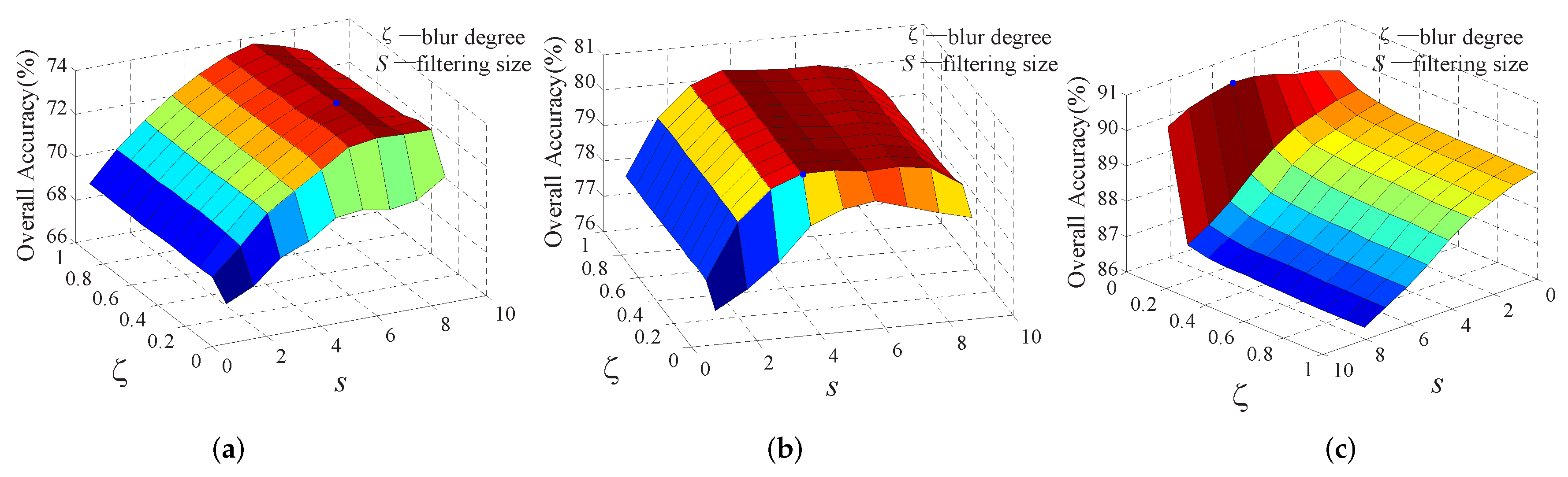
First, the influence of the filtering size, s, and the blur degree, $\zeta$, on the classification performance are show in Figure 5 In the experiments on Indian Pines and Pavia University data sets, s varies from 1 to 9 and $\zeta$ varies from 0 to 1, while for the Salinas data set, s varies from 12 to 20 and $\zeta$ varies from 0 to 1. It can be seen that if s and $\zeta$ are too large, the OA of the method will decline greatly. That is, too-large s and $\zeta$ will cause the image to be smoothed out considerably, and some small-scale targets will be misclassified. When the s and $\zeta$ are too small, the performance of the method also decreased significantly. The reason for this result is that edge preserving filtering is a local filtering process, and the smaller the window, the smaller the range of spatial information considered in probability optimization. s and $\zeta$ should take the appropriate value. Therefore, the parameters s and $\zeta$ setting as (s = 7, $\zeta$ = 0.4), (s = 4, $\zeta$ = 0.1), and (s = 17, $\zeta$ = 0) for the Indian Pines, Pavia University, Salinas data sets, respectively, in this paper can obtain the highest OA.

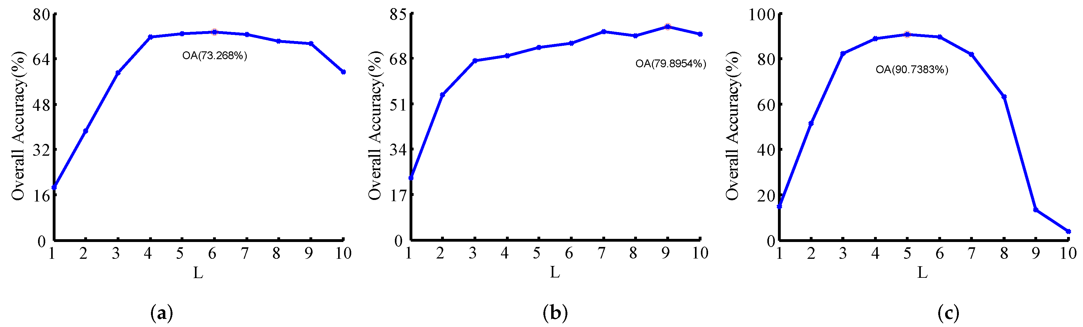
Then, the influence of L (which varies from 1 to 10) to the performance is shown in Figure 6. It can be seen that the accuracy of the proposed method increases gradually as L increases. This means that the proposed method can effectively extract the multi-scale characteristics of HSI for classification. For the proposed method, L is separately set to 6, 9, and 5 as the default parameters for the three data sets, respectively.

3.4. Classification Results with Different Numbers of Training Samples

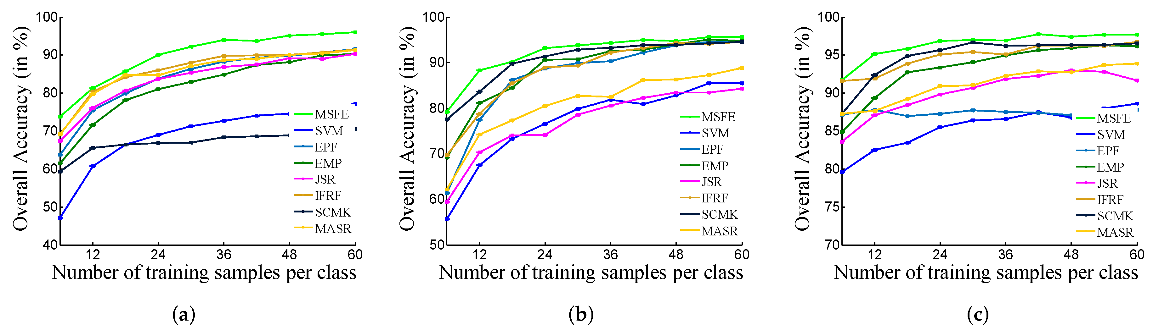
The classification performance to eight methods with different training samples on the three data sets is shown in Figure 7. In the three figures, the number of training samples for all methods increased from 6 to 60. It can be observed that when the number of training samples changes, the proposed method significantly improved the classification accuracies in comparison with other approaches.

4. Conclusions

In this paper, the MSFE method was presented for the classification of HSIs. This method contains two important strategies: First, the Gaussian pyramid decomposition strategy was employed to achieve multi-scale analysis of images. The proposed method can capture spatial texture features of different scales, and thus targets of different scales can be classified more effectively. Second, by using the EPF algorithm to optimize the probability map, the proposed method can produce a smoother appearance in a homogeneous regions. Therefore, the details and the near-edge area of the image can be better identified. Furthermore, experimental results demonstrate the proposed method outperforms other classification methods in term of accuracy, especially when the number of training samples is quite limited. In future work, multi-scale feature fusion will be integrated into the MSFE to further improve classification accuracy. In addition, we can further solve the problem of classification accuracy loss when the number of samples is small.

References

- Chen, C.H.; Ho, P.G. Statistical pattern recognition in remote sensing. Pattern Recognit. 2008, 41, 2731–2741. [Google Scholar] [CrossRef]
- Fernandes, L.A.F.; Oliveira, M.M. Corrigendum to Real-time line detection through an improved hough transform voting scheme. Pattern Recognit. 2008, 41, 299–314. [Google Scholar] [CrossRef]
- Brook, A.; Dor, E.B. Quantitative detection of settled dust over green canopy using sparse unmixing of airborne hyperspectral data. IEEE J. Sel. Top. Appl. Earth Obs. Remote Sens. 2016, 9, 884–897. [Google Scholar] [CrossRef]
- Yuan, Y.; Wang, Q.; Zhu, G. Fast hyperspectral anomaly detection via high-order 2-D crossing filter. IEEE Trans. Geosci. Remote Sens. 2015, 53, 620–630. [Google Scholar] [CrossRef]
- Lee, M.A.; Huang, Y.; Yao, H.; Thomson, S.J. Determining the effects of storage on cotton and soybean leaf samples for hyperspectral analysis. IEEE J. Sel. Top. Appl. Earth Obs. Remote Sens. 2014, 7, 2562–2570. [Google Scholar] [CrossRef]
- Dalponte, M.; Orka, H.O.; Gobakken, T.; Gianelle, D.; Nasset, E. Tree species classification in boreal forests with hyperspectral data. IEEE Trans. Geosci. Remote Sens. 2013, 51, 2632–2645. [Google Scholar] [CrossRef]
- Tarabalka, Y.; Chanussot, J.; Benediktsson, J.A. Segmentation and classification of hyperspectral images using watershed transformation. Pattern Recognit. 2010, 43, 2367–2379. [Google Scholar] [CrossRef] [Green Version]
- Li, Y.; Xie, W.; Li, H. Hyperspectral image reconstruction by deep convolutional neural network for classification. Pattern Recognit. 2017, 63, 371–383. [Google Scholar] [CrossRef]
- He, N.; Fang, L.; Li, S.; Plaza, A.; Plaza, J. Remote sensing scene classification using multilayer stacked covariance pooling. IEEE Trans. Geosci. Remote Sens. 2018, 56, 6899–6910. [Google Scholar] [CrossRef]
- Tu, B.; Zhang, X.; Kang, X.; Zhang, G.; Li, S. Density Peak-based Noisy Label Detection for Hyperspectral Image Classification. IEEE Trans. Geosci. Remote Sens. 2019, 57, 1573–1584. [Google Scholar] [CrossRef]
- Tu, B.; Zhang, X.; Kang, X.; Wang, J.; Benediktsson, J.A. Spatial Density Peak Clustering for Hyperspectral Image Classification with Noisy Labels. IEEE Trans. Geosci. Remote Sens. 2019. [Google Scholar] [CrossRef]
- Ghamisi, P.; Yokoya, N.; Li, J.; Liao, W.; Liu, S.; Plaza, J.; Rasti, B.; Plaza, A. Advances in Hyperspectral Image and Signal Processing: A Comprehensive Overview of the State of the Art. IEEE Geosci. Remote Sens. Mag. 2017, 5, 37–78. [Google Scholar] [CrossRef] [Green Version]
- Gao, L.; Li, J.; Khodadadzadeh, M.; Plaza, A.; Zhang, B.; He, Z.; Yan, H. Subspace-based support vector machines for hyperspectral image Classification. IEEE Geosci. Remote Sens. Lett. 2015, 12, 349–353. [Google Scholar]
- Bruzzone, L.; Chi, M.; Marconcini, M. A novel transductive SVM for semisupervised Classification of remote-sensing images. IEEE Trans. Geosci. Remote Sens. 2006, 44, 3363–3373. [Google Scholar] [CrossRef]
- Wang, X.Z.; He, Q.; Chen, D.G.; Yeung, D. A genetic algorithm for solving the inverse problem of support vector machines. Neurocomputing 2005, 68, 225–238. [Google Scholar] [CrossRef]
- Melgani, F.; Bruzzone, L. Classification of hyperspectral remote sensing images with support vector machines. IEEE Trans. Geosci. Remote Sens. 2004, 42, 1778–1790. [Google Scholar] [CrossRef] [Green Version]
- Li, J.; Bioucas-Dias, J.; Plaza, A. Spectral-spatial hyperspectral image segmentation using multinomal subspace multinomial logistic regression and Markov random fields. IEEE Trans. Geosci. Remote Sens. 2012, 50, 809–823. [Google Scholar] [CrossRef]
- Li, J.; Bioucas-Dias, J.; Plaza, A. Semi-supervised hyperspectral image segmentation using multinomial logistic regression with active learning. IEEE Trans. Geosci. Remote Sens. 2010, 48, 4085–4098. [Google Scholar]
- Li, J.; Bioucas-Dias, J.; Plaza, A. Semi-supervised hyperspectral image Classification using soft sparse multinomial logistic regression. IEEE Geosci. Remote Sens. Lett. 2013, 10, 318–322. [Google Scholar]
- Zhu, J.; Fang, L.; Ghamis, P. Deformable convolutional neural networks for hyperspectral image classification. IEEE Geosci. Remote Sens. Lett. 2018, 15, 1254–1258. [Google Scholar] [CrossRef]
- Ye, J. Adaptive control of nonlinear PID-based analog neural networks for a nonholonomic mobile robot. Neurocomputing 2018, 71, 1561–1565. [Google Scholar] [CrossRef]
- Fang, L.; Liu, G.; Li, S.; Ghamisi, P.; Benediktsson, J.A. Hyperspectral Image Classification with Squeeze Multibias Network. IEEE Trans. Geosci. Remote Sens. 2019. [Google Scholar] [CrossRef]
- Camps-Valls, G.; Bruzzone, L. Kernel-based methods for hyperspectral image classification. IEEE Trans. Geosci. Remote Sens. 2005, 43, 1351–1362. [Google Scholar] [CrossRef] [Green Version]
- Fauvel, M.; Chanussot, J.; Benediktsson, J.A. A spatial-spectral Kernel-based approach for the classification of remote-sensing images. Pattern Recognit. 2012, 45, 381–392. [Google Scholar] [CrossRef]
- Rajan, S.; Ghosh, J.; Crawford, M.M. An active learning approach to hyperspectral data classification. IEEE Trans. Geosci. Remote Sens. 2008, 46, 1231–1242. [Google Scholar] [CrossRef]
- Tuia, D.; Ratle, F.; Pacifici, F.; Kanevski, M.F.; Emery, W.J. Active learning methods for remote sensing image classification. IEEE Trans. Geosci. Remote Sens. 2009, 47, 2218–2232. [Google Scholar] [CrossRef]
- Ghamisi, P.; Plaza, J.; Chen, Y.; Li, J.; Plaza, A.J. Advanced Spectral Classifiers for Hyperspectral Images: A review. IEEE Geosci. Remote Sens. Mag. 2017, 5, 8–32. [Google Scholar] [CrossRef]
- Liu, L.; Chen, C.L.P.; You, X.; Tang, Y.Y.; Zhang, Y.; Li, S. Mixed noise removal via robust constrained sparse representation. IEEE Trans. Circuits Syst. Video Technol. 2018, 28, 2177–2189. [Google Scholar] [CrossRef]
- Han, J.; He, S.; Qian, X.; Wang, D.; Guo, L.; Liu, T. An object-oriented visual saliency detection framework based on sparse coding representations. IEEE Trans. Circuits Syst. Video Technol. 2013, 23, 2009–2021. [Google Scholar] [CrossRef]
- Chen, Y.; Nasrabadi, N.M.; Tran, T.D. Hyperspectral image classification using dictionary-based sparse representation. IEEE Trans. Geosci. Remote Sens. 2011, 49, 3973–3985. [Google Scholar] [CrossRef]
- Chen, Y.; Nasrabadi, N.M.; Tran, T.D. Hyperspectral image classification via kernel sparse representation. IEEE Trans. Geosci. Remote Sens. 2013, 51, 217–231. [Google Scholar] [CrossRef]
- Tu, B.; Zhang, X.; Wang, J.; Zhang, G.; Ou, X. Spectral–Spatial Hyperspectral Image Classification via Non-local Means Filtering Feature Extraction. Sens. Imaging 2018, 19, 1–11. [Google Scholar] [CrossRef]
- Tu, B.; Yang, X.; Li, N.; Ou, X.; He, W. Hyperspectral Image Classification via Superpixel Correlation Coefficient Representation. IEEE J. Sel. Top. Appl. Earth Obs. Remote Sens. 2018, 11, 4113–4127. [Google Scholar] [CrossRef]
- Kang, X.; Li, S.; Benediktsson, J.A. Feature extraction of hyperspectral images with image fusion and recursive filtering. IEEE Geosci. Remote Sens. Lett. 2014, 52, 3742–3752. [Google Scholar] [CrossRef]
- Kang, X.; Li, S.; Benediktsson, J.A. Spectral-spatial hyperspectral image classification with edge-preserving filtering. IEEE Trans. Geosci. Remote Sens. 2014, 52, 2666–2677. [Google Scholar] [CrossRef]
- Tu, B.; Zhang, X.; Kang, X.; Zhang, G.; Wang, J.; Wu, J. Hyperspectral image classification via fusing Correlation Coefficient and Joint Sparse Representation. IEEE Geosci. Remote Sens. Lett. 2018, 15, 340–344. [Google Scholar] [CrossRef]
- Camps-Valls, G.; Gomez-Chova, L.; Munoz-Mari, J.; Vila-Frances, J.; Calpe-Maravilla, J. Composite kernels for hyperspectral image classification fication. IEEE Trans. Geosci. Remote Sens. Lett. 2006, 3, 93–97. [Google Scholar] [CrossRef]
- Li, J.; Marpu, P.R.; Plaza, A.; Bioucas-Dias, J.M.; Benediktsson, J.A. Generalized composite kernel framework for hyperspectral image classification. IEEE Trans. Geosci. Remote Sens. 2013, 51, 4816–4829. [Google Scholar] [CrossRef]
- Fang, L.; Li, S.; Kang, X.; Benediktsson, J.A. Spectral-spatial hyperspectral image classification via multiscale adaptive spare representation. IEEE Trans. Geosci. Remote Sens. 2014, 52, 7738–7749. [Google Scholar] [CrossRef]
- Xia, J.; Chanussot, J.; Du, P.; He, X. Spectral-spatial classification for hyperspectral data using rotation forests with local feature extraction and Markov random fields. IEEE Trans. Geosci. Remote Sens. 2015, 53, 2532–2546. [Google Scholar] [CrossRef]
- Zhang, L.; Tao, D.; Huang, X. On combining multiple features for hyperspectral remote sensing image classification. IEEE Trans. Geosci. Remote Sens. 2012, 50, 879–893. [Google Scholar] [CrossRef]
- Li, W.; Chen, C.; Su, H.; Du, Q. Local binary patterns and extreme learning machine for hyperspectral imagery classification. IEEE Trans. Geosci. Remote Sens. 2015, 53, 3681–3693. [Google Scholar] [CrossRef]
- Yang, Y.; Song, J.; Huang, Z.; Ma, Z.; Alexander, G. Hauptmann multi-feature fusion via hierarchical regression for multimedia analysis. IEEE Trans. Multimed. 2013, 15, 572–581. [Google Scholar] [CrossRef]
- Peng, J.; Zhou, Y.; Chen, C. Region-kernel-based support vector machines for hyperspectral image classification. IEEE Trans. Geosci. Remote Sens. 2015, 53, 4810–4824. [Google Scholar] [CrossRef]
- Zhao, W.; Guo, Z.; Yue, J.; Zhang, X.; Luo, L. On combining multiscale deep learning features for the classification of hyperspectral remote sensing imagery. Int. J. Remote Sens. 2015, 36, 3368–3379. [Google Scholar] [CrossRef]
- Benediktsson, J.A.; Pesaresi, M.; Amason, K. Classification and feature extraction for remote sensing images from urban areas based on morphological transformations. Trans. Geosci. Remote Sens. 2003, 41, 1940–1949. [Google Scholar] [CrossRef] [Green Version]
- He, N.; Paoletti, E.M.; Haut, J.M.; Li, S.; Plaza, A.; Plaza, J. Feature Extraction With Multiscale Covariance Maps for Hyperspectral Image Classification. IEEE Trans. Geosci. Remote Sens. 2019, 57, 755–769. [Google Scholar] [CrossRef]
- Mirzapour, F.; Ghassemian, H. Multiscale Gaussian Derivative Functions for Hyperspectral Image Feature Extraction. IEEE Geosci. Remote Sens. Lett. 2016, 13, 525–529. [Google Scholar] [CrossRef]
- Li, S.; Hao, Q.; Kang, X.; Benediktsson, J.A. Gaussian pyramid based multiscale feature fusion for hyperspectral image classification. IEEE J. Sel. Top. Appl. Earth Obs. Remote Sens. 2018, 11, 3312–3324. [Google Scholar] [CrossRef]
- Prasad, S.; Bruce, L.M. Limitations of pincipal components analysis for hyperspectral target recognition. IEEE Geosci. Remote Sens. Lett. 2008, 5, 625–629. [Google Scholar] [CrossRef]
- Benediktsson, J.A.; Palmason, J.A.; Sveninsson, J.R. Classification of hyperespectral data from urban ares based on extended morphological profiles. IEEE Trans. Geosci. Remote Sens. 2005, 43, 480–491. [Google Scholar] [CrossRef]
- Fang, L.; Li, S.; Duan, W.; Ren, J.; Benediktsson, J.A. Classification of hyperspectral images by exploiting spectral–spatial information of superpixel via multiple kernels. IEEE Trans. Geosci. Remote Sens. 2015, 53, 6663–6674. [Google Scholar] [CrossRef]
Figure 1.
Schematic diagram of the proposed classification method. Support vector machine (SVM), edge-preserving filtering (EPF), Gaussian pyramid.
Figure 2.
Indian Pines image: (a) three-band color composite, (b) reference data, (c) class names, Classification maps (Indian Pines) obtained by (d) the SVM method (48.63%), (e) the extended morphological profiles (EMP) method (61.42%), (f) the EPF method (63.76%), (g) the image fusion and recursive filtering (IFRF) method (68.97%), (h) the joint sparse representation (JSR) method (68.57%), (i) the superpixel-based classification via multiple kernels (SCMK) method (59.32%), (j) the MASR method (69.62%), and (k) the multi-scale feature extraction (MSFE) method (73.92%).
Figure 3.
University of Pavia image: (a) three-band color composite, (b) reference data, (c) class names, Classification maps (University of Pavia) obtained by (d) the SVM method (55.69%), (e) the EMP method (67.93%), (f) the EPF method (61.32%), (g) the IFRF method (66.82%), (h) the JSR method (63.69%), (i) the SCMK method (77.36%), (j) the MASR method (61.57%), and (k) the MSFE method (81.35%).
Figure 4.
Salinas image: (a) Three-band color composite, (b) Reference data, (c) Class names, Classification maps (Salinas) obtained by (d) the SVM method (79.56%), (e) the EMP method (85.32%), (f) the EPF method (85.44%), (g) the IFRF method (88.91%), (h) the JSR method (83.61%), (i) the SCMK method (88.40%), (j) the MASR method (87.47%), and (k) the MSFE method (92.08%).
Figure 5.
Analysis of the effect of the parameters s (the filtering size) and (blur degree). (a) Indian Pines dataset. (b) University of Pavia dataset. (c) Salinas dataset.
Figure 6.
Analysis of the effect of the parameter L (the number of layers in the Gaussian pyramid). (a) Indian Pines dataset. (b) University of Pavia dataset. (c) Salinas dataset.
Figure 7.
Classification results with varying number of training samples by SVM, EMP, EPF, IFRF, JSR, SCMK, MASR, and the proposed method, MSFE. (a) Indian Pines dataset, (b) University of Pavia dataset, (c) Salinas dataset.