Letter

Scattering Characterization of Obliquely Oriented Buildings from PolSAR Data Using Eigenvalue-Related Model

1
State Key Laboratory of Complex Electromagnetic Environment Effects on Electronics and Information System, National University of Defense Technology, Changsha 410073, China
2
National Innovation Institute of Technology, Beijing 100091, China
*
Author to whom correspondence should be addressed.
Submission received: 10 February 2019 / Revised: 28 February 2019 / Accepted: 5 March 2019 / Published: 10 March 2019
(This article belongs to the Section Remote Sensing Image Processing)

Abstract

:
Scattering characterization of obliquely oriented buildings (OOBs) from polarimetric synthetic aperture radar (PolSAR) data is challenging since the general double-bounce scattering does not support their dominant scattering mechanism. In this paper, a physical scattering model combining the eigenvalues of coherency matrix is proposed to characterize the scattering of OOBs. The coherency matrix is first operated by eigenvalue decomposition and a refined OOB descriptor is presented based on these eigenvalues. Considering the actual proportions of co-polarization and cross-polarization components, the descriptor is then adopted to modify the matrix elements of the well-known cross scattering model, thus introducing the OOB scattering model. Finally, strategies of model parameter solution are designed and the involved decomposition is complete accordingly. The proposed method is tested on spaceborne and airborne PolSAR data and the results confirm its effectiveness, which clearly call for further research and application.

Graphical Abstract

1. Introduction

Scattering behavior understanding is a bridge between the collected polarimetric synthetic aperture radar (PolSAR) data and real applications [1,2,3,4]. Concerning this, numerous studies have gone into model-based decomposition (MBD) of the coherency matrix as the summation of several scattering components and the product MBDs proposed by Freeman [1] and Yamaguchi [2] are widely applied. As a specific data processing method, the MBD provides insights into the scattering mechanism over the scenes with different land covers and thus is still developing at a considerable speed.
Despite all of this, outputs from the MBDs are sometimes confusing when discrimination between obliquely oriented buildings (OOBs) and natural areas is made. For an OOB whose main scattering center is at an oblique direction with respect to the radar illumination (its orientation angular domain approximately ranges between 22.5° and 45° (or between −45° and −22.5°) [4]), intense cross-polarization powers instead of co-polarization powers will be induced [4,5,6,7]. Simultaneously, there also exist significant cross-polarization responses in natural areas. This phenomenon, known as the overestimation of volume scattering (OVS), can lead to scattering mechanism ambiguity as well as misinterpretation. In reaction to this issue, many approaches are proposed and have met with varying degrees of success [8,9,10,11,12,13,14,15,16,17,18,19,20,21]. One well-known technique is adopting the mathematical operation for the input coherency matrix. Representative examples of such works include non-negative eigenvalue decomposition (NNED) [8,9,10] and orientation angle compensation (OAC) [11,12,13]. However, the NNED generally has high computational complexity due to the pick of the optimal coefficient. While for the OAC, it sometimes produces non-robust results when dealing with buildings with large orientation angles. On this occasion, studies are inclined to introduce more sophisticated scattering models [14,15,16,17,18,19,20,21]. Among them, the cross scattering model (CSM) [21] dedicates to separate powers caused by OOBs from the overall cross-polarization components and achieves the relatively high property of scattering characterization. Nevertheless, the CSM is data-dependent and still suffers severe OVS to some extent.
To address the aforementioned issues, an OOB scattering model which integrates the CSM and the eigenvalues of coherency matrix is proposed in this paper. The main work includes the following aspects. First, an eigenvalue-related OOB descriptor proposed by [22] is revisited and a refinement is put forward on this basis. Second, the refined OOB descriptor is utilized to construct a scattering model (OOB scattering model), which considers the actual proportions of co-polarization and cross-polarization components. Third, to achieve the accurate scattering contribution estimation, strategies of modular calculation and quadratic discriminant with root determination are elaborately designed for the involved MBD. Finally, different spaceborne and airborne PolSAR data are utilized and the effectiveness of the proposed method is comprehensively verified.

2. Methodology

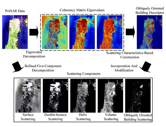
2.1. Refined OOB Descriptor

Subject to the reciprocity condition, the acquired full polarimetric information can be expressed in the form of the coherency matrix as
[ T ] = k 3 p k 3 p H = [ T 11 T 12 T 13 T 21 T 22 T 23 T 31 T 32 T 33 ]
where k 3 p represents the Pauli vector. The superscript H and the notation indicate the conjugate transpose and ensemble averaging, respectively. The eigenvalues and eigenvectors of the 3-D Hermitian coherency matrix can be computed with
[ T ] = i = 1 3 λ i u i u i H
where the real numbers λ i are the eigenvalues and u i is the unit orthogonal eigenvector.
Recently, Quan et al. [22] proposed a robust descriptor to characterize the polarimetric characteristics of OOBs via the combination of eigenvalues. The robustness reflects in that the eigenvalues for different building orientations are roll-invariant. Considering that the eigenvalues have been ordered as λ 1 > λ 2 > λ 3 , the descriptor of OOBs is defined as
D OOB = D DP D RD ( 1 D PA ) = λ 3 4 λ 3 SPAN ( 1 λ 1 λ 2 SPAN 3 λ 3 )
where SPAN is total power of the radar return. D DP , D RD , and D PA denotes the measurement of depolarization, randomness, and polarimetric asymmetry, respectively. According to [22], the descriptor is constructed based on the following facts.
(1) In practical applications, a large cross-polarization component is typically associated with significant depolarization of the scattered energy [23]. The minimum eigenvalue λ 3 is actually a measurement of completely depolarized component of the total power [24]. When λ 3 = 0 , the entire return is polarized. However, when λ 3 > 0 , the depolarized component increases. As a result, OOBs have high value of λ 3 .
(2) Influenced by the oblique orientation, double reflection signal no longer travels back to the radar for OOBs. This results in that other direct reflections from the ground begin to dominate and the signals appear more random [22]. Therefore, OOBs have a high amount of randomness.
(3) Through plentiful experiments, Quan et al. [22] found that buildings approximately aligned with the flight trajectory generally have medium polarimetric asymmetry, while natural areas have high polarimetric asymmetry. On the contrary, OOBs have a low level of polarimetric asymmetry.
The descriptor has been proven to highlight the polarimetric characteristics of OOBs effectively. Nevertheless, there are still risks that the misjudgment can occur in some natural areas if they have very high amounts of depolarization and randomness. Given this, we refine the descriptor as follows
C OOB = 4 λ 3 2 SPAN ( 1 λ 1 λ 2 SPAN 3 λ 3 ) 2 .
Expectedly, the square of the second term can reduce the impact of natural areas with high depolarization and randomness since polarimetric asymmetry in OOBs is significantly smaller than that in natural areas [22]. It needs to be emphasized that the square processing is ascertained through plentiful tests on datasets with different sensors and wavebands. Too high exponent will cause remarkable loss of local information of OOBs. In addition, notice that the descriptor is constructed mainly from a qualitative perspective and therefore, the impact of eigenvalue estimation is insignificant.

2.2. OOB Scattering Model

The CSM is derived according to the fact that a cosine squared distribution is generally used for vertical structures [21]. According to the algebraic model of cross scattering, it consists of the approximatively equal amount of co-polarization component (the T 22 term) and cross-polarization component (the T 33 term). Specifically, the maximum difference between the elements is only ± 1 / 15 [21]. However, in real OOB landforms, cross-polarization power is found to be more intense than co-polarization power [4,5,6,7]. In this case, we incorporate the refined OOB descriptor C OOB and propose the scattering model of an OOB as follows
[ T ] OOB = [ 0 0 0 0 O 22 0 0 0 O 33 ]
where
O 22 = C OOB C OOB + C OOB M C OOB + ξ , O 33 = C OOB M C OOB + ξ C OOB + C OOB M C OOB + ξ .
The notation M denotes the maximum value of C OOB . ξ , and is an infinitesimally small positive number which prevents the denominator from becoming zero. As noticed, the matrix form of the proposed model is designed to be identical to the one of the CSM since it can effectively extract the cross scattering feature. However, the model is an optimization in two aspects. First, without any priori information, the original T 22 term in [21] is replaced with C OOB , which represents a certain amount of co-polarization components in OOBs. Second, in consideration of the cross-polarization component in OOBs, the original T 33 term in [21] is replaced with C OOB / ( M C OOB ) . The rationale lies in that C OOB / ( M C OOB ) is much greater than C OOB , which corresponds to the relative proportion of co-polarization and cross-polarization components. Even though C OOB is large in OOBs, the above manipulation always makes the co-polarization component small compared to the cross-polarization component. Thus, the cross-polarization component is greatly elevated. Finally, the matrix elements are rigorously normalized to [0, 1] since there is no definite range of C OOB . On comparing the relative magnitudes of O 22 and O 33 , these approximations are more reasonable and closer to the actuals. In addition, instead of directly fitting the original T 33 term to C OOB , we believe that the proposed adjustment is more promising.

2.3. Model Solution

In a similar manner as [18,21], the coherency matrix is decomposed as a weighted sum of five kinds of basic scattering (surface, double-bounce, helix, volume, and OOB scattering, respectively), i.e.,
[ T ] = f S [ T ] S + f D [ T ] D + f H [ T ] H + f V [ T ] V + f O [ T ] OOB .
where f S , f D , f C , f V , and f O are scattering coefficients to be computed. [ T ] S , [ T ] D , [ T ] H , and [ T ] V are the corresponding specific models and their mathematical forms as given as [1,2]
[ T ] S = [ 1 β 0 β | β | 2 0 0 0 0 ] , [ T ] D = [ | α | 2 α 0 α 1 0 0 0 0 ] [ T ] H = 1 2 [ 0 0 0 0 1 ± j 0 j 1 ] , [ T ] V = 1 4 [ 2 0 0 0 1 0 0 0 1 ] .
Thereinto, α and β denote the model parameters of double-bounce scattering and surface scattering, respectively. j represents the imaginary unit and the positive (negative) sign indicates right (left) helix scattering. After careful mathematical operations, a set of equations can be derived with the aforementioned models, i.e.,
f S + f D | α | 2 + f V 2 = T 11 f S | β | 2 + f D + f V 4 + f H 2 + f O O 22 = T 22 f V 4 + f H 2 + f O O 33 = T 33 f S β + f D α = T 12 f H 2 = | Im ( T 23 ) | .
To solve the underdetermined problem, assumptions need to be made to reduce the unknowns. Similar to [21], one of the unknowns can be fixed according to the sign of T 11 T 22 + f H / 2 . If T 11 T 22 + f H / 2 > 0 , then f D = 0 , assuming the surface scattering is dominant in the remaining matrix (subtracting the helix scattering component from the input coherency matrix), otherwise f S = 0 , assuming the double-bounce scattering is dominant in the remaining matrix. Nevertheless, although the expressions shown in (8) are compact, the direct achievement of the analytic solutions is complicated. In fact, if C OOB is small, the f O O 22 term can be directly omitted. If C OOB is large and close to its maximum value, the f O O 22 term can also be omitted since the normalization always makes O 22 negligible. In this case, the equation sets are solvable and the following expressions can be acquired via modular calculation, i.e.,
T 11 T 22 + f H 2 > 0 : Re ( β ) = Re ( T 12 ) f S , Im ( β ) = Im ( T 12 ) f S T 11 T 22 + f H 2 < 0 : Re ( α ) = Re ( T 12 ) f D , Im ( α ) = Im ( T 12 ) f D .
Further apply Equations (8) and (9) to obtain
T 11 T 22 + f H 2 > 0 > 0 : f S 2 + ( 2 T 22 f H T 11 ) f S 2 | T 12 | 2 = 0 T 11 T 22 + f H 2 > 0 < 0 : 2 f D 2 + ( T 11 + f H 2 T 22 ) f D | T 12 | 2 = 0.
T 11 T 22 + f H 2 > 0 : f S 2 + ( 2 T 22 f H T 11 ) f S 2 | T 12 | 2 = 0 T 11 T 22 + f H 2 < 0 : 2 f D 2 + ( T 11 + f H 2 T 22 ) f D | T 12 | 2 = 0.
Apparently, the quadratic discriminant in Equation (10) is always positive, ensuring that the quadratic equation has two roots. This splits in the following operation: (1) If the larger root is negative, f S (or f D ) is forced to zero; (2) If the larger root is positive while the smaller root is negative, f S (or f D ) is equal to the larger root; and (3) If the smaller root is positive, f S (or f D ) is still equal to the larger root. This constrains the estimation of f V from not being overwhelming.
Once the surface or double-bounce scattering coefficient is determined, the rest scattering coefficients can be computed. Their expressions are given as
T 11 T 22 + f H 2 > 0 : f D = 0 , f H = 2 | Im ( T 23 ) | f S = ( 2 T 22 f H T 11 ) 2 + 8 | T 12 | 2 ( 2 T 22 f H T 11 ) 2 f V = 2 ( T 11 f S ) , f O = 4 T 33 2 f H f V 4 O 33 .
or
T 11 T 22 + f H 2 > 0 : f S = 0 , f H = 2 | Im ( T 23 ) | f D = ( T 11 + f H 2 T 22 ) 2 + 8 | T 12 | 2 ( T 11 + f H 2 T 22 ) 4 f V = 2 ( 2 T 22 2 f D f H ) , f O = 4 T 33 2 f H f V 4 O 33 .
As a result, the corresponding scattering contributions P S , P D , P H , P V , and P O are estimated as
P S = f S ( 1 + | β | 2 ) , P D = f D ( 1 + | α | 2 ) P H = f H , P O = f O , P V = SPAN P S P D P H P O .

3. Experimental Results

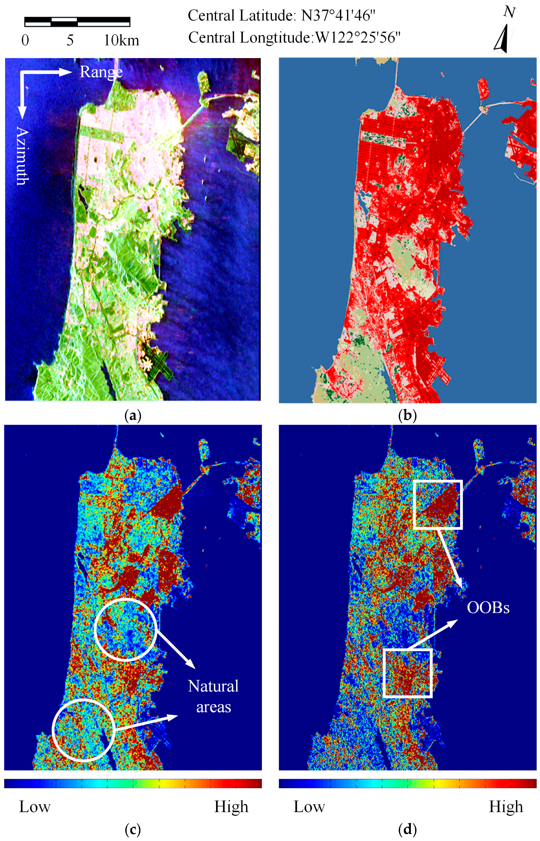
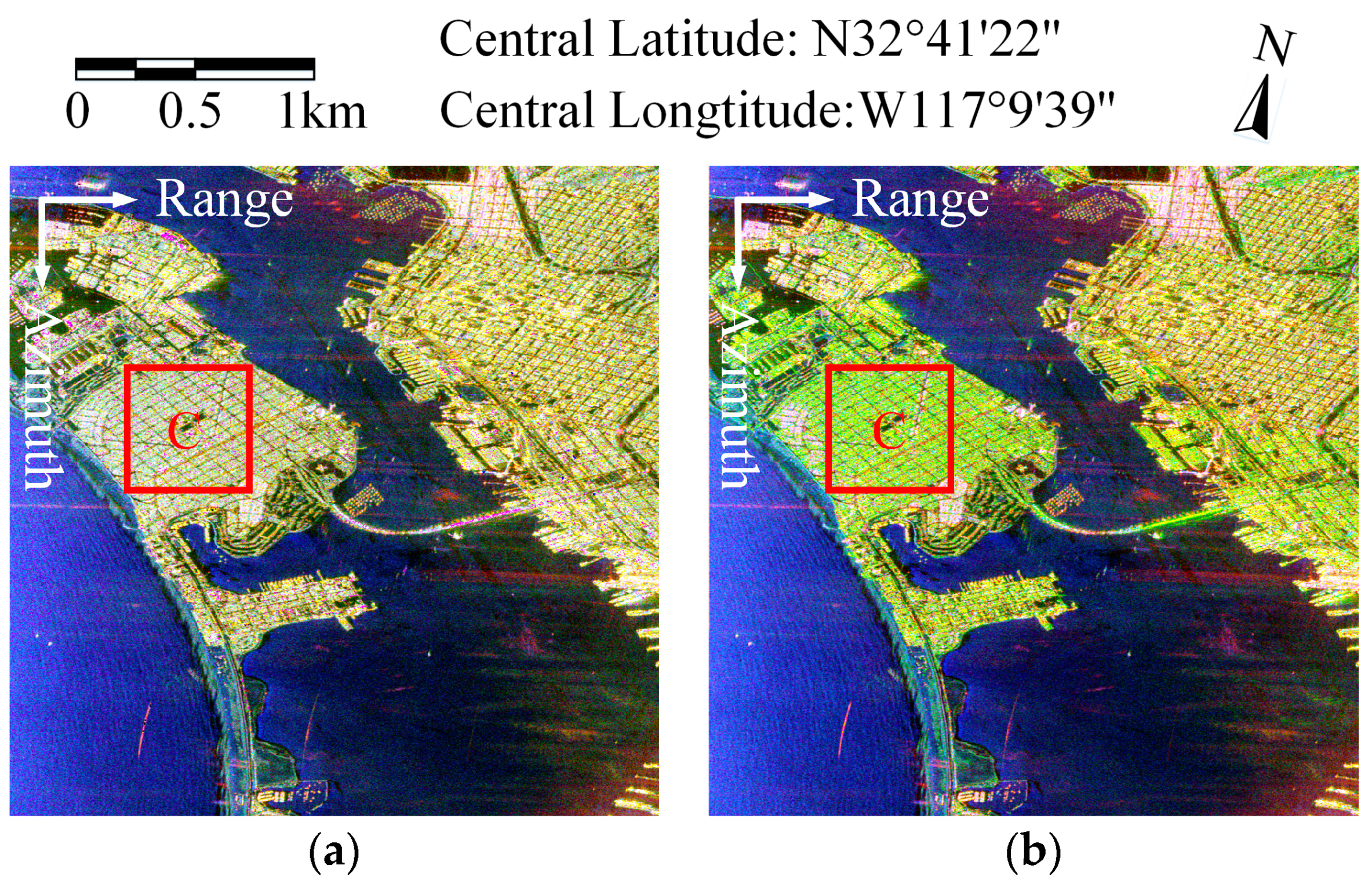
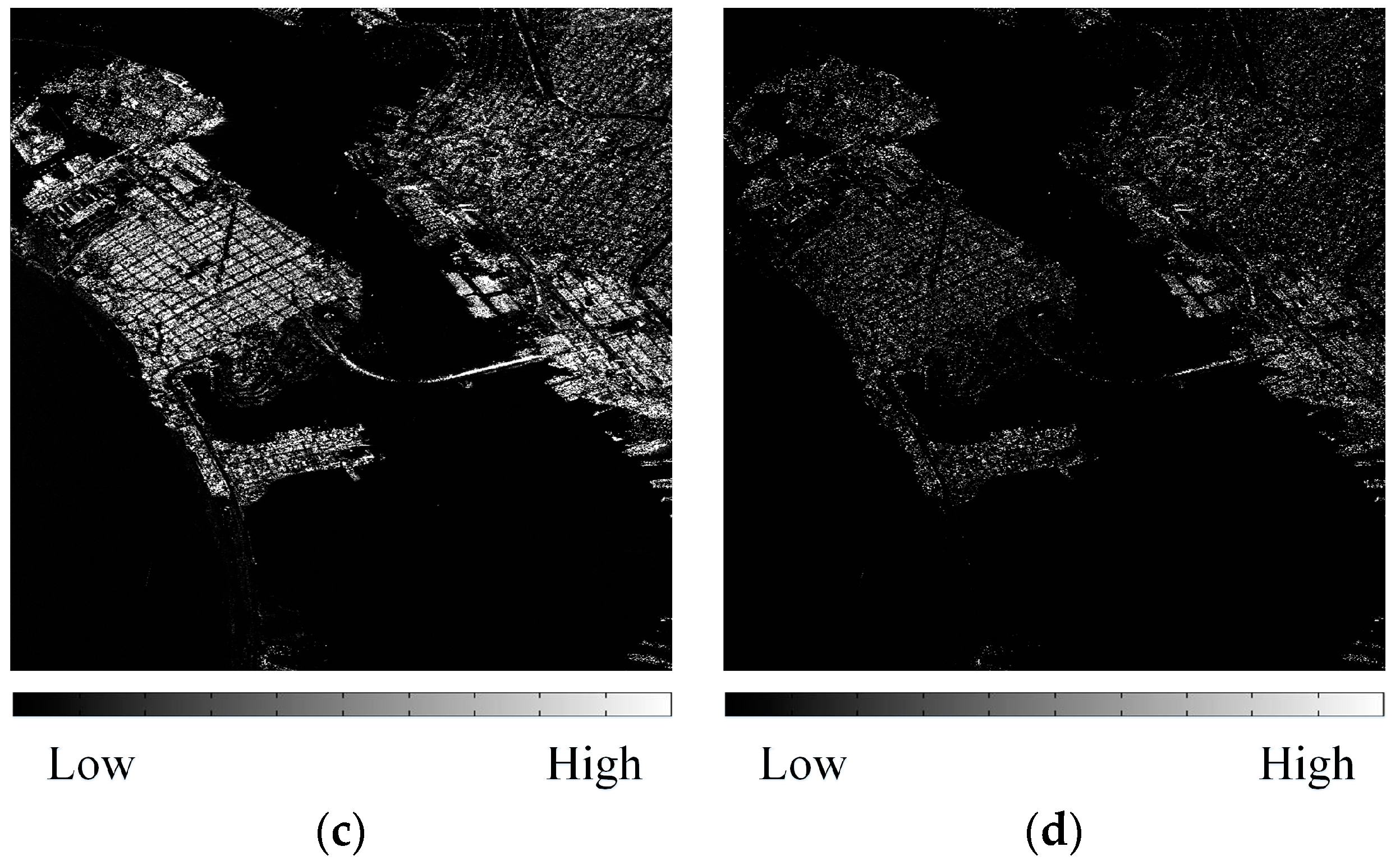
3.1. Validation on Spaceborne Data

The spaceborne PolSAR data are acquired over a test site in San Francisco, USA. Figure 1a displays the Radarsat-2 C-band Pauli color-coded image, where the red channel denotes the T 22 term, the green channel denotes the T 33 term, and the blue channel denotes the T 11 term. The ensemble average is performed with factors 10 and 5 in the azimuth and range direction, respectively. Accordingly, the resulting resolution corresponds to 24.1 m × 23.7 m in the ground area. To evaluate the performance of the proposed method, the National Land Cover Database 2016 (NLCD 2016) [25] is used as the ground reference image, where pixels in red represent the actual distribution of urban areas. It can be seen that various types of urban landforms are included ranging from streets, highways, and bridges to buildings with different orientations. Therefore, the effectiveness of the proposed method can be properly evaluated.
Figure 1c,d illustrates the comparison of the original and refined descriptors. On inspection, it is clear that OOBs are shown by brown regions while other land covers are colored blue. This explains that the polarimetric characteristics of OOBs are notably highlighted by the descriptor. However, some natural areas (outlined by the circles) and OOBs have approximate values with respect to the original OOB descriptor. This increases the risk that natural areas may be treated as OOBs. Meanwhile, by further considering the square of polarimetric asymmetry, natural areas are obviously impaired while OOBs are retained (see the rectangular areas). This helps for better representation of OOBs. In addition to this, one can notice that the depth of color indicates the oblique extent of buildings. The darker the color, the larger the building orientation.
The color conventions of decomposition results are used and given in Figure 2, where the red channel denotes the urban scattering (the sum of double-bounce, helix, and the OOB/cross scattering), the green channel denotes volume scattering, and the blue channel denotes surface scattering. In addition, the OOB and cross scattering components of the proposed and CSM methods are presented individually in Figure 2. Expectedly, cross scattering powers are remarkable for OOBs but negligible for other land covers. Nevertheless, apart from some special OOBs (see the rectangular area), cross scattering powers stay at a relatively low level for most OOBs. This may increase the risk of the emergence of the OVS. Meanwhile, the proposed method generates more promising results, which is reflected in the brightness of almost all OOBs (e.g., the circular area). It gives a full-scale observation and is able to find more of the smaller OOB regions though few are missed out. These signify that the OOB scattering is remarkable and valid. One may notice that the color composite results produced from the proposed method are similar to those from the CSM. However, this is not the case and the quantitative analysis will illustrate it in the following.
To quantitatively compare the cross and OOB scattering models, different districts (the black rectangular areas in Figure 2) are demarcated for further analysis. District A covers high rise OOBs which tilted by about 37° from the flight trajectory [3]. District B is a residential area which includes buildings approximately aligned with the flight trajectory (AABs). The corresponding normalized scattering power statistics are shown in Table 1 and Table 2. Thereinto, three cases of the CSM with different OAs are involved in the evaluation. Specifically, when the OA is 0°, the CSM degenerates into the one in [19]. When the OA is 22.5°, the CSM have the same form as the one in [20]. The model in [19] indicates that the orientations of rotated dihedral structures formed by buildings mainly centered about zero degree, while the model in [20] demonstrates that the orientations of man-made rotated diplane structures prefer to follow a random distribution.
With respect to the CSM, it is intuitive that different OAs results in varying estimation of cross scattering powers. Unfortunately, the CSM methods still suffer the deficiency in the OVS for district A (65.97%, 65.93%, and 65.95%, respectively). While for the proposed method, a significant decrease in volume scattering alongside a simultaneous increase in surface scattering can be observed. On one hand, this explains that the proposed method can moderate the OVS remarkably. On the other hand, a large proportion of the decrements of volume scattering are transferred to the increments of surface scattering. This can be interpreted as odd-bounce returns from roofs, streets, and structures between two buildings, which are more reasonable and conform to reality. Another notable observation is that small percentages of double-bounce scattering are produced. This is in compliance with the fact that the cross-polarization component is much greater than the co-polarization component in OOBs.
What is noteworthy is that the OOB scattering is significantly increased (about 15%) compared to the CSM methods. This explains that the proposed method can not only preserve, but also enhance the cross-polarization components in OOBs. In this case, the building scattering can be characterized with more certainty by further emphasizing the OOB scattering. For district B, it is apparent that the dominant mechanism is double-bounce scattering (about 65% for all these methods). Moreover, the scattering powers all remain at the same level. This indicates that the proposed method can improve the scattering characteristics of OOBs while keep the estimation accurate for AABs.
To further highlight the differences between the OOB and cross scattering components, the yellow rectangular areas in Figure 2 are zoomed in and pixels of the bridge (the yellow dashed rectangular areas in Figure 3) are selected. The extent of scattering components’ change on the pixels is given in Figure 3. The red and black dotted lines denote the averaged cross and OOB scattering powers, respectively. It can be seen that results generated by the CSM are distributed with more discontinuous regions, introducing underestimated and erroneous scattering contributions. From Figure 3c, it is noteworthy that OOB scattering powers are observably greater than cross scattering powers, resulting in the clear identification of the bridge.

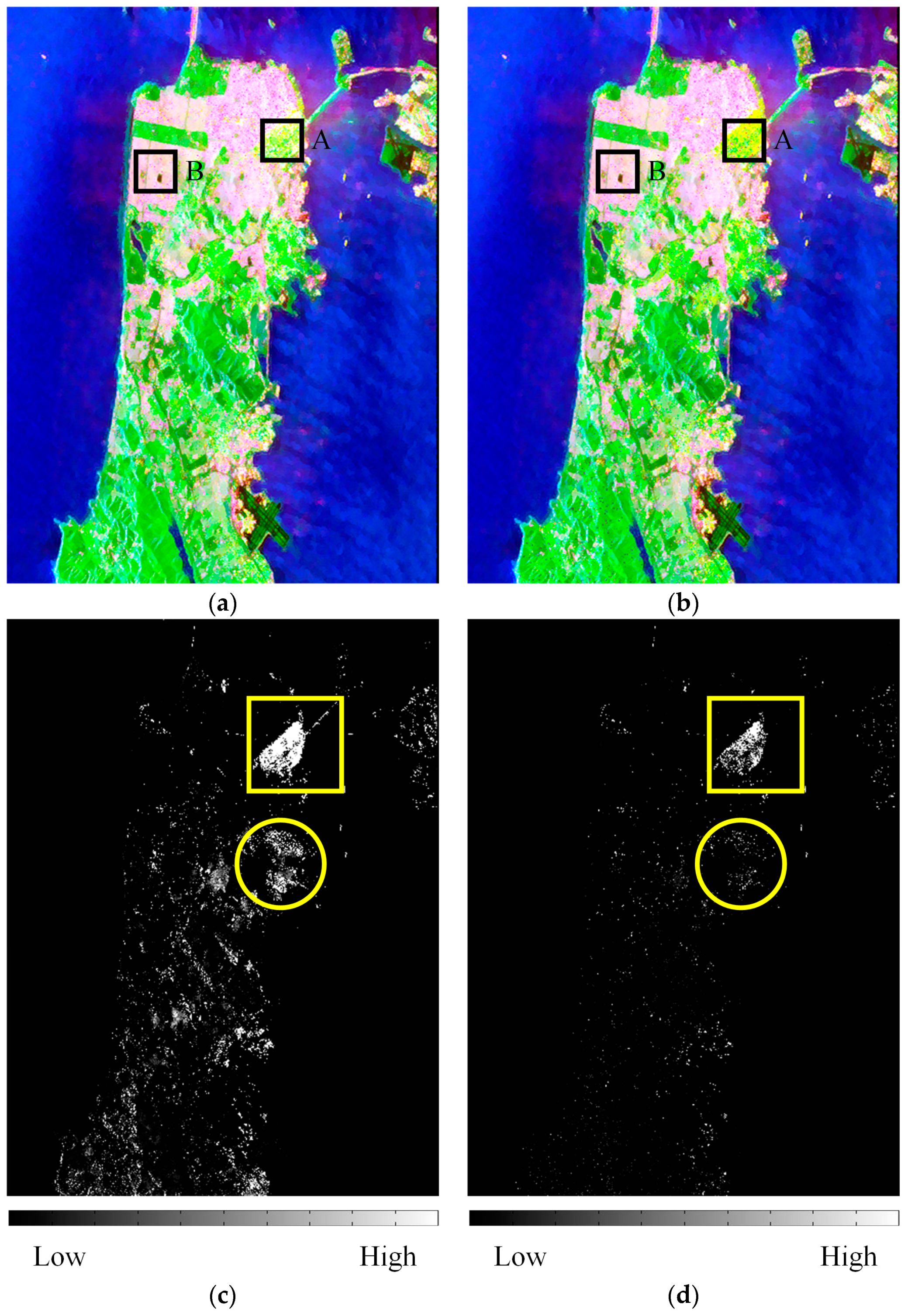
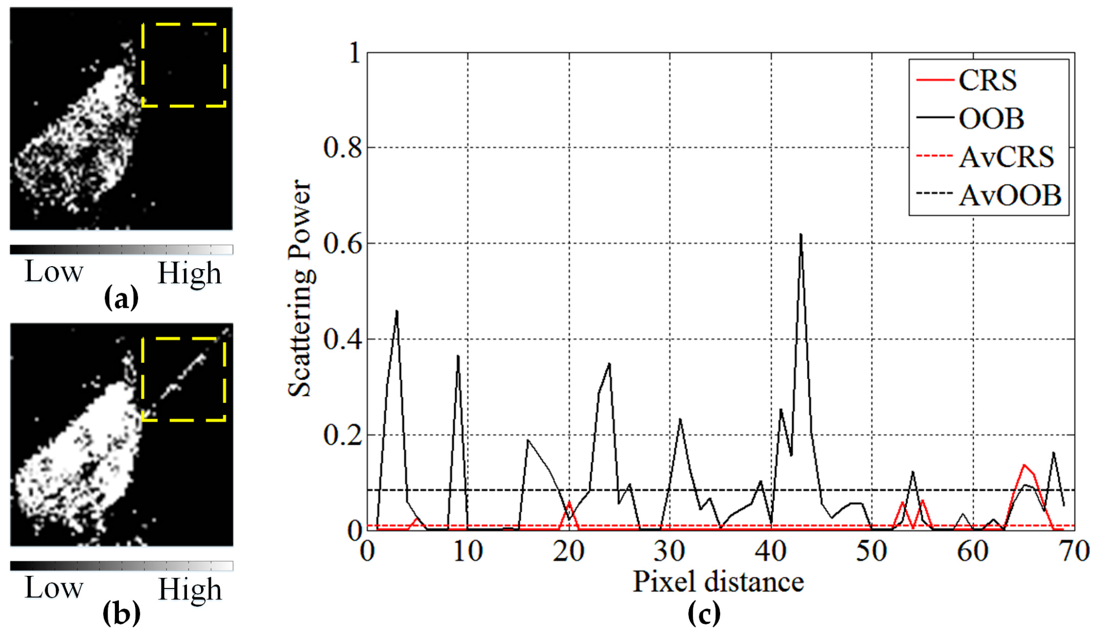
3.2. Further Inspection on Airborne Data

The airborne data acquired by the L-band AIRSAR are located in San Diego, USA. It has a resolution with 9.25 m in azimuth direction and 3.33 m in range direction. Figure 4 presents the results of the proposed method and the CSM, respectively.
As can be observed, for urban areas comprising AABs (pixels in red), they clearly show a dominance of double-bounce scattering mechanism. Meanwhile regarding OOBs, it can be seen from Figure 4c that the majority of pixels exhibits OOB scattering behavior and the contours of OOBs are veraciously highlighted. Whereas, for the cross scattering the powers are quite low and most of the OOB details are lost. On comparing Figure 4a with Figure 4b, it is apparent that the results generated by the proposed method appear light yellow rather than green, which means that there exist remarkable OOB scattering and less volume scattering in OOBs.
For quantitative analysis purpose, a low-rise OOB district (the red rectangular areas in Figure 4) is selected and the normalized scattering power statistics are given in Table 3. It is obvious that the proposed method outperforms the CSM methods in moderating the OVS and enhancing the cross-polarization components of OOBs. In addition, the odd-bounce contributions (the surface scattering) by the proposed method are about 20% more than those by the CSM methods, which are attributed to radar returns from streets and roofs. The above observations agree well with those from the spaceborne decomposition, which further confirm the effectiveness of the proposed method.

4. Conclusions

Vast sections of OOBs appear to be dominated by volume scattering in traditional MBD approaches since small variations in building orientation lead to significant drops in co-polarization power. Concerning such orientation sensitivity, this paper proposes an OOB scattering model by integrating the roll-invariant parameters, i.e., the eigenvalues of coherency matrix. The modeling is implemented by modifying the matrix elements of the CSM in consideration of the actual proportions of co-polarization and cross-polarization components. On this basis, model parameter solutions are further designed for the estimation of scattering powers. Two PolSAR data with different sensor configurations and geographic locations are utilized and the efficacy of the proposed method has been objectively assessed. Experimental results demonstrate that the OVS is remarkably moderated and more reasonable surface scattering is enhanced. More importantly, the OOB scattering components are further enhanced, which enable better characterization of OOB scattering.

Author Contributions

S.Q. is responsible for the design of the methodology, experimental data collection and processing, and preparation of the manuscript. D.X. analyzed the data, B.X., and C.H. helped analyze and discuss the results. G.K. is responsible for the technical support of the manuscript.

Funding

This research was funded by National Natural Science Foundation of China, grant numbers 61701508 and 41801236.

Acknowledgments

The authors would like to thank the editors and the anonymous reviewers for their constructive comments that significantly improved the quality of this paper. The authors would also like to thank NASA/JPL for the AIRSAR data. Radarsat-2 data has been downloaded from the Radarsat-2 website.

Conflicts of Interest

The authors declare no conflict of interest. The founding sponsors had no role in the design of the study; in the collection, analyses, or interpretation of data; in the writing of the manuscript, and in the decision to publish the results.

References

  1. Freeman, A.; Durden, S.L. A three-component scattering model for polarimetric SAR data. IEEE Trans. Geosci. Remote Sens. 1998, 36, 963–973. [Google Scholar] [CrossRef]
  2. Yamaguchi, Y.; Moriyama, T.; Ishido, M.; Yamada, H. Four-component scattering model for polarimetric SAR image decomposition. IEEE Trans. Geosci. Remote Sens. 2005, 43, 1699–1706. [Google Scholar] [CrossRef]
  3. Atwood, D.K.; Thirion-Lefevre, L. Polarimetric Phase and Implications for Urban Classification. IEEE Trans. Geosci. Remote Sens. 2018, 56, 1278–1289. [Google Scholar] [CrossRef]
  4. Chen, S.; Ohki, M.; Shimada, M.; Sato, M. Deorientation Effect Investigation for Model-Based Decomposition Over Oriented Built-Up Areas. IEEE Geosci. Remote Sens. Lett. 2013, 10, 273–277. [Google Scholar] [CrossRef]
  5. Guinvarc’h, R.; Thirion-Lefevre, L. Cross-Polarization Amplitudes of Obliquely Orientated Buildings with Application to Urban Areas. IEEE Geosci. Remote Sens. Lett. 2017, 14, 1913–1917. [Google Scholar] [CrossRef]
  6. Quan, S.; Xiang, D.; Xiong, B.; Hu, C.; Kuang, G. A Hierarchical Extension of General Four-Component Scattering Power Decomposition. Remote Sens. 2017, 9, 856. [Google Scholar] [CrossRef]
  7. Chen, S.; Wang, X.; Xiao, S.; Sato, M. General Polarimetric Model-Based Decomposition for Coherency Matrix. IEEE Trans. Geosci. Remote Sens. 2014, 52, 1843–1855. [Google Scholar] [CrossRef]
  8. Van Zyl, J.J.; Arii, M.; Kim, Y. Model-based decomposition of polarimetric SAR covariance matrices constrained for nonnegative eigenvalues. IEEE Trans. Geosci. Remote Sens. 2011, 49, 3452–3459. [Google Scholar] [CrossRef]
  9. Cui, Y.; Yamaguchi, Y.; Yang, J.; Park, S.E.; Kobayashi, H.; Singh, G. Three-Component Power Decomposition for Polarimetric SAR Data Based on Adaptive Volume Scatter Modeling. Remote Sens. 2012, 4, 1559–1572. [Google Scholar] [CrossRef] [Green Version]
  10. Cui, Y.; Yamaguchi, Y.; Yang, J.; Kobayashi, H.; Park, S.E.; Singh, G. On complete model-based decomposition of polarimetric SAR coherency matrix data. IEEE Trans. Geosci. Remote Sens. 2014, 52, 1991–2001. [Google Scholar] [CrossRef]
  11. Lee, J.S.; Ainsworth, T.L. The Effect of Orientation Angle Compensation on Coherency Matrix and Polarimetric Target Decompositions. IEEE Trans. Geosci. Remote Sens. 2011, 49, 53–64. [Google Scholar] [CrossRef]
  12. An, W.; Xie, C.; Yuan, X.; Cui, Y.; Yang, J. Four-component decomposition of polarimetric SAR images with deorientation. IEEE Geosci. Remote Sens. Lett. 2011, 8, 1090–1094. [Google Scholar] [CrossRef]
  13. Chen, S.; Wang, X.; Sato, M. Uniform Polarimetric Matrix Rotation Theory and Its Applications. IEEE Trans. Geosci. Remote Sens. 2014, 52, 4756–4770. [Google Scholar] [CrossRef]
  14. Arii, M.; van Zyl, J.J.; Kim, Y. Adaptive model-based decomposition of polarimetric SAR covariance matrices. IEEE Trans. Geosci. Remote Sens. 2011, 49, 1104–1113. [Google Scholar] [CrossRef]
  15. Antropov, O.; Rauste, Y.; Häme, T. Volume scattering modeling in PolSAR decompositions: Study of ALOS PALSAR data over boreal forest. IEEE Trans. Geosci. Remote Sens. 2011, 49, 3838–3848. [Google Scholar] [CrossRef]
  16. Lee, J.S.; Ainsworth, T.L.; Wang, Y. Generalized polarimetric model-based decompositions using incoherent scattering models. IEEE Trans. Geosci. Remote Sens. 2014, 52, 2474–2491. [Google Scholar] [CrossRef]
  17. Xie, Q.; Ballester-Berman, D.; Lopez-Sanchez, J.M.; Zhu, J.; Wang, C. On the Use of Generalized Volume Scattering Models for the Improvement of General Polarimetric Model-Based Decomposition. Remote Sens. 2017, 9, 117. [Google Scholar] [CrossRef]
  18. Zhang, L.; Zou, B.; Cai, H.; Zhang, Y. Multiple-Component Scattering Model for Polarimetric SAR Image Decomposition. IEEE Geosci. Remote Sens. Lett. 2008, 5, 603–607. [Google Scholar] [CrossRef]
  19. Sato, A.; Yamaguchi, Y.; Singh, G.; Park, S.E. Four-component scattering power decomposition with extended volume scattering model. IEEE Geosci. Remote Sens. Lett. 2012, 9, 166–170. [Google Scholar] [CrossRef]
  20. Hong, S.H.; Wdowinski, S. Double-Bounce Component in Cross-Polarimetric SAR from a New Scattering Target Decomposition. IEEE Trans. Geosci. Remote Sens. 2014, 52, 3039–3051. [Google Scholar] [CrossRef]
  21. Xiang, D.; Ban, Y.; Su, Y. Model-Based Decomposition With Cross Scattering for Polarimetric SAR Urban Areas. IEEE Geosci. Remote Sens. Lett. 2015, 12, 2496–2500. [Google Scholar] [CrossRef]
  22. Quan, S.; Xiong, B.; Xiang, D.; Zhao, L.; Zhang, S.; Kuang, G. Eigenvalue-Based Urban Area Extraction Using Polarimetric SAR Data. IEEE J. Sel. Top. Appl. Earth Observ. Remote Sens. 2018, 11, 458–471. [Google Scholar] [CrossRef]
  23. Van Zyl, J.J.; Kim, Y. Synthetic Aperture Radar Polarimetry; Wiley: Pasadena, CA, USA, 2011; pp. 85–158. ISBN 978-7-11-809289-9. [Google Scholar]
  24. Lee, J.S.; Pottier, E. Polarimetric Radar Imaging: From Basics to Applications; Taylor & Francis: Boca Raton, FL, USA, 2009; pp. 85–158. ISBN 978-1-42-005497-2. [Google Scholar]
  25. Yang, L.; Jin, S.; Danielson, P.; Homer, C.; Gass, L.; Bender, S.M.; Casei, A.; Costello, C.; Dewitz, J.; Fry, J.; et al. A new generation of the United States National Land Cover Database: Requirements, research priorities, design, and implementation strategies. ISPRS J. Photogramm. Remote Sens. 2018, 146, 108–123. [Google Scholar] [CrossRef]
Figure 1. Radarsat-2 C-band data and the obliquely oriented building descriptors. (a) Pauli color-coded image (red: The T 22 term, green: The T 33 term, and blue: The T 11 term). (b) Ground reference from the National Land Cover Database 2016. (c) The original OOB descriptor. (d) The refined OOB descriptor.
Remotesensing 11 00581 g001
Figure 2. Decomposition results. (a,b) Color composite results of the proposed and cross scattering model methods, respectively (red: Urban scattering, green: Volume scattering, and blue: Surface scattering). (c,d) OOB and cross scattering components of the proposed and CSM methods, respectively.
Remotesensing 11 00581 g002
Figure 3. Detailed excerpts from the decomposed yellow rectangular areas in Figure 3. (a) Cross scattering component. (b) OOB scattering component. (c) Profile of scattering components from the bridge, where CRS, OOB, AvCRS, and AvOOB are the abbreviations of cross scattering, OOB scattering, averaged cross scattering, and averaged OOB scattering, respectively.
Remotesensing 11 00581 g003
Figure 4. Results of AIRSAR L-band data. (a,b) Color composite results of the proposed and CSM methods, respectively (red: Urban scattering, green: Volume scattering, and blue: Surface scattering) (c,d) OOB and cross scattering components of the proposed and CSM methods, respectively.
Remotesensing 11 00581 g004aRemotesensing 11 00581 g004b
Table 1. Normalized scattering power statistics for district A.
ProposedCSM (with Specific OA)
22.5°Adaptive
Surface scattering20.49%1.77%1.75%1.76%
Double-bounce scattering4.19%4.25%4.25%4.25%
Volume scattering32.37%65.97%65.93%65.95%
Helix scattering6.44%6.44%6.44%6.44%
OOB/Cross scattering36.51%21.57%21.63%21.60%
Table 2. Normalized scattering power statistics for district B.
ProposedCSM (with Specific OA)
22.5°Adaptive
Surface scattering24.86%25.02%25.01%25.02%
Double-bounce scattering63.56%63.53%63.50%63.52%
Volume scattering9.42%9.10%9.11%9.11%
Helix scattering1.73%1.73%1.73%1.73%
OOB/Cross scattering0.43%0.62%0.65%0.62%
Table 3. Normalized scattering power statistics for district C.
ProposedCSM (with Specific OA)
22.5°Adaptive
Surface scattering43.85%23.26%23.25%23.26%
Double-bounce scattering11.06%12.45%12.44%12.45%
Volume scattering18.10%50.28%50.24%50.27%
Helix scattering9.47%9.47%9.47%9.47%
OOB/Cross scattering17.53%4.54%4.59%4.56%

