A New Global Total Electron Content Empirical Model


1
School of Civil and Architectural Engineering, Shandong University of Technology, Zibo 255000, China
2
Sate Key Laboratory of Space Weather, Chinese Academy of Sciences, Beijing 100190, China
3
State Key Laboratory of Geodesy and Earth’s Dynamics, Institute of Geodesy and Geophysics, Chinese Academy of Sciences, Wuhan 430077, China
4
School of Geodesy and Geomatics, Wuhan University, Wuhan 430079, China
*
Author to whom correspondence should be addressed.
Remote Sens. 2019, 11(6), 706; https://0-doi-org.brum.beds.ac.uk/10.3390/rs11060706
Submission received: 10 January 2019
/
Revised: 11 March 2019
/
Accepted: 21 March 2019
/
Published: 24 March 2019
(This article belongs to the Special Issue Latest Results and Developments in GNSS Ionosphere Theory, Methods, Technologies, Applications and Future Challenges)
Abstract
:Research on total electron content (TEC) empirical models is one of the important topics in the field of space weather services. Global TEC empirical models based on Global Ionospheric Maps (GIMs) TEC data released by the International GNSS Service (IGS) have developed rapidly in recent years. However, the accuracy of such global empirical models has a crucial restriction arising from the non-uniform accuracy of IGS TEC data in the global scope. Specifically, IGS TEC data accuracy is higher on land and lower over the ocean due to the lack of stations in the latter. Using uneven precision GIMs TEC data as a whole for model fitting is unreasonable. Aiming at the limitation of global ionospheric TEC modelling, this paper proposes a new global ionospheric TEC empirical model named the TECM-GRID model. The model consists of 5183 sections, corresponding to 5183 grid points (longitude 5°, latitude 2.5°) of GIM. Two kinds of single point empirical TEC models, SSM-T1 and SSM-T2, are used for TECM-GRID. According to the locations of grid points, the SSM-T2 model is selected as the sub-model in the Mid-Latitude Summer Night Anomaly (MSNA) region, and SSM-T1 is selected as the sub-model in other regions. The fitting ability of the TECM-GRID model for modelling data was tested in accordance with root mean square (RMS) and relative RMS values. Then, the TECM-GRID model was validated and compared with the NTCM-GL model and Center for Orbit Determination in Europe (CODE) GIMs at time points other than modelling time. Results show that TECM-GRID can effectively describe the Equatorial Ionization Anomaly (EIA) and the MSNA phenomena of the ionosphere, which puts it in good agreement with CODE GIMs and means that it has better prediction ability than the NTCM-GL model.

1. Introduction
The ionospheric model is widely used in GNSS systems to provide real-time ionospheric delay correction for single frequency users. Different GNSS systems use different ionospheric models. For instance, the Klobuchar model is used in GPS systems to correct ionospheric delay for single frequency users. The model regards the night ionospheric delay as a constant with a value of 5 ns and the daytime delay as a positive part of the cosine function. The Beidou navigation satellite system (BDS) also introduces a modified Klobuchar model [1,2]. Single-frequency users of the European Galileo Satellite Navigation System (Galileo) use the broadcast NeQuick-Gal model to correct ionospheric delay. The ionospheric coefficients of the NeQuick-Gal model are updated and transmitted daily by broadcast ephemeris. Other kinds of ionospheric models, such as the empirical models, are expressed as a series of empirical formulas based on ionospheric observations recorded over a long period of time as a modelling database. The International Reference Ionosphere (IRI) [3] and NeQuick/NeQuick2 [4,5] are the well-known empirical ionospheric models, which are available for estimating ionospheric total electron content (TEC) and three-dimensional electron profiles.
With the continuous improvement of GNSS systems, the network of GNSS tracking stations in regions is becoming increasingly dense globally. The widely distributed GNSS tracking station provides a new way for TEC data acquisition worldwide. Since 1998, the International GNSS Service (IGS) has used GNSS tracking station data to calculate and provide global ionospheric maps (GIMs). Thus far, more than 20 years of GIMs TEC time series data are available. On the one hand, GIMs TEC data offer a novel means for the study of the temporal and spatial variation of the global ionosphere. On the other hand, it also presents a reliable database for the establishment of TEC empirical models. In recent years, the single station/regional/global TEC empirical models based on global ionospheric TEC grid, single station, or regional GNSS-TEC data have been developed. Mao et al. [6] established an empirical ionospheric TEC model over the Wuhan Station by using TEC data from 1980 to 1990 and empirical orthogonal function analysis. Huang and Yuan [7] proposed a short-term ionospheric TEC prediction over a single station by utilising an improved radial basis function (RBF) neural network algorithm based on the Gauss mixture model. Huang et al. [8] created a one-hour ionospheric TEC prediction model for a single station by using Back Propagation (BP) artificial neural network algorithm optimized by a genetic algorithm. Hajra et al. [9] developed a single-station ionospheric TEC empirical model using TEC observations over the Calcutta station in India from 1980 to 1990. Jakowski [10] suggested an empirical ionospheric TEC model NTCM-EU suitable for Europe by using the non-linear least squares method. Using GPS-TEC data and spherical harmonic function, Opperman et al. [11] generated an empirical ionospheric TEC model for South Africa. Mao et al. [12] built an empirical ionospheric TEC model for China by using GPS data and empirical orthogonal function analysis from 1996 to 2004. Bouya et al. [13] produced an empirical ionospheric TEC model for the Australian region using spherical coronal harmonic analysis. Habarulema et al. [14,15] developed an empirical ionospheric TEC model for South Africa using a neural network algorithm. Chen et al. [16] established an empirical TEC model for the North American region by using empirical orthogonal function analysis.
Empirical orthogonal function analysis, the neural network algorithm and non-linear least squares method are widely used in the study of a single station/region’s ionospheric TEC empirical models, which provides important reference for the establishment of global ionospheric TEC empirical models. Jakowski et al. [17] developed a new global ionospheric empirical model (NTCM-GL) using GIMs TEC data provided by the CODE analysis centre of IGS from 1998 to 2007. The NTCM-GL model contains only 12 coefficients (which are fitted by the non-linear least squares method) and 8 fixed constants, and the root mean square (RMS) of model residuals is 7.5 TECU. The NTCM-GL model has been developed to act as a background model for TEC estimates and mapping. Therefore, for said model to be robust and fast, the number of coefficients is only 12. Given that NTCM-GL covers a full solar cycle, the spatial resolution is clearly limited from the outset compared with other models using many more coefficients, like IRI models. Mukhtarov et al. [18,19] transformed the CODE TEC data from 1999 to 2011 into a modified magnetic dip latitude coordinate system, then a new global TEC empirical model was established by using the non-linear least squares method. The model contains 4374 coefficients for estimation, and the standard deviation of the model residuals is 3.387 TECU. Moreover, the model can reconstruct the EIA and the Weddell Sea anomaly structure. Andonov [20] developed a new global ionospheric TEC empirical model using 1999–2011 CODE TEC data and non-linear least squares method. On the basis of previous studies [18,19], Mukhtarov et al. [21] proposed another global ionospheric TEC hybrid prediction model using CODE TEC data. In addition, on the basis of GIMs TEC data provided by the JPL analysis centre of IGS, other empirical models of global ionospheric TEC [22,23] were generated by empirical orthogonal function analysis.
However, such global empirical models based on IGS GIMs TEC data may have the following restrictions: (1) the accuracy of GIMs TEC data is not uniform all over the world. The uneven distribution of IGS stations globally is characterized by density in land areas, and scarcity or even absence in ocean areas, which results in global inconsistency in the accuracy of GIMs TEC data. GIMs TEC data often fails to accurately describe the variation characteristics of TEC in areas where few or no stations are present. Sometimes TEC even has negative values. Moreover, using GIMs TEC data with relatively poor accuracy in ocean areas as the modelling data set and applying global non-linear least squares equal weight processing will also reduce the accuracy of the model in the land area, especially in the continental area surrounded by oceans in the southern hemisphere. (2) Empirical models have certain deficiencies in describing some ionospheric anomalies. Many abnormal phenomena occur in the ionosphere, which only exists in some local areas. Examples include the EIA which occurs at 10–15° north and south of the magnetic equator while the MSNA occurs in the vicinity of the Weddell Sea in the southern hemisphere, in north-eastern China, northern Japan, and in the northern hemisphere [24,25,26,27,28]. Global ionospheric TEC empirical models based on GIMs TEC data cannot accurately describe the characteristics of ionospheric variation without considering these anomalies and modelling them reasonably. On the other hand, the ionospheric correction models commonly used in GNSS systems also have deficiencies in predicting some ionospheric anomalies. For example, the Klobuchar model can only correct 50–60% of the ionospheric delay [29], cannot accurately describe the details of TEC changes [30], and cannot construct EIA and MSNA phenomena. Some empirical models also show similar situations in describing anomalies. For example, the NeQuick2 model can describe EIA phenomena [30], but it does not effectively reproduce MSNA phenomena [31]. The descriptive ability of the NeQuick2 model for EIA is also closely related to the intensity of solar activity. For example, Venkatesh et al. [32] studied the descriptive ability of the NeQuick2 model for TEC variation over equatorial and low latitude regions by comparing NeQuick2-TEC with the measured GPS-TEC data during the 24th solar cycle. The NeQuick2 model can predict the location and peak values of EIA at low solar activity level, but it underestimates the peak value of EIA with the increase of solar activity intensity.
In this paper, a new idea of a modelling pattern is proposed, which can not only effectively avoid the problem of inconsistent accuracy of modelling data, but can also appropriately deal with ionospheric anomalies. The idea of the model is that the world is divided into 5183 grid points (longitude 5° × latitude 2.5°), and the TEC empirical models are established at each grid point, thereby totalling 5183 sections. Accordingly, the proposed model is named the TECM-GRID model.
2. Modelling Methods
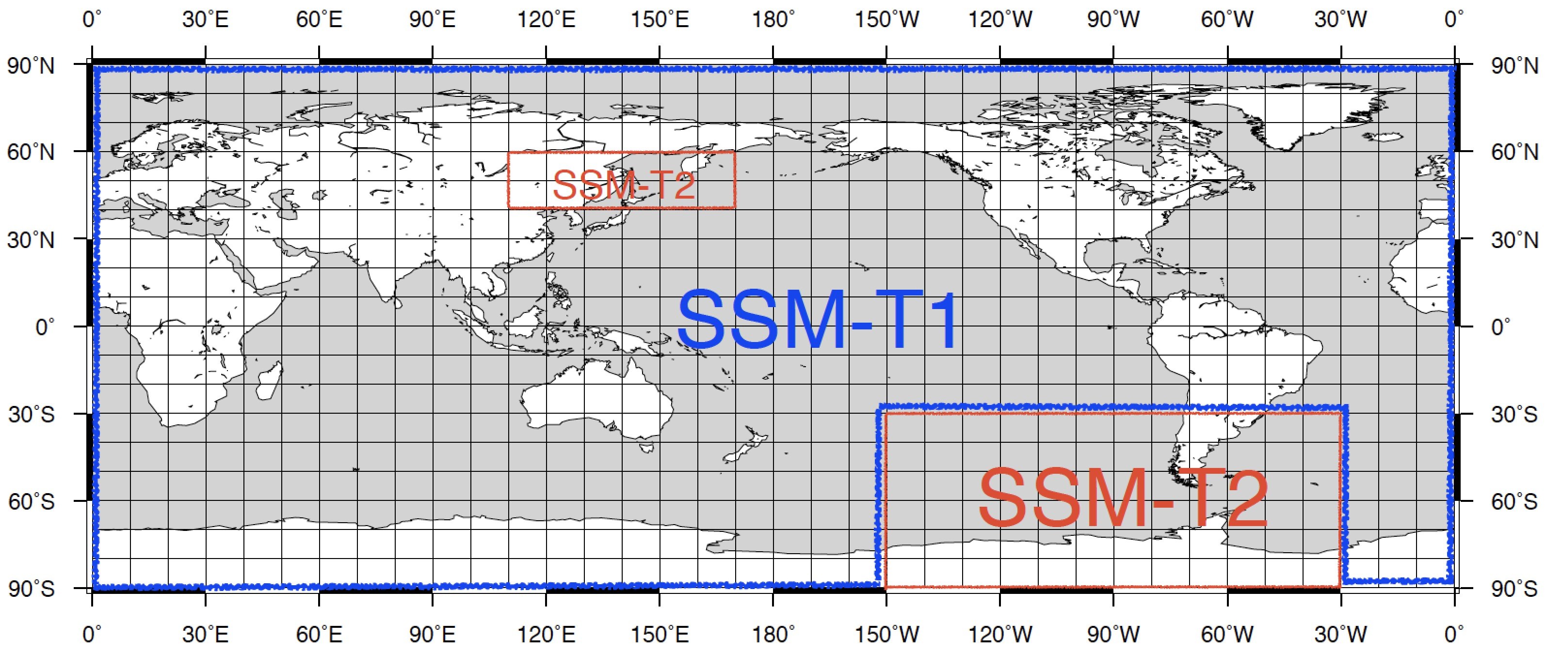
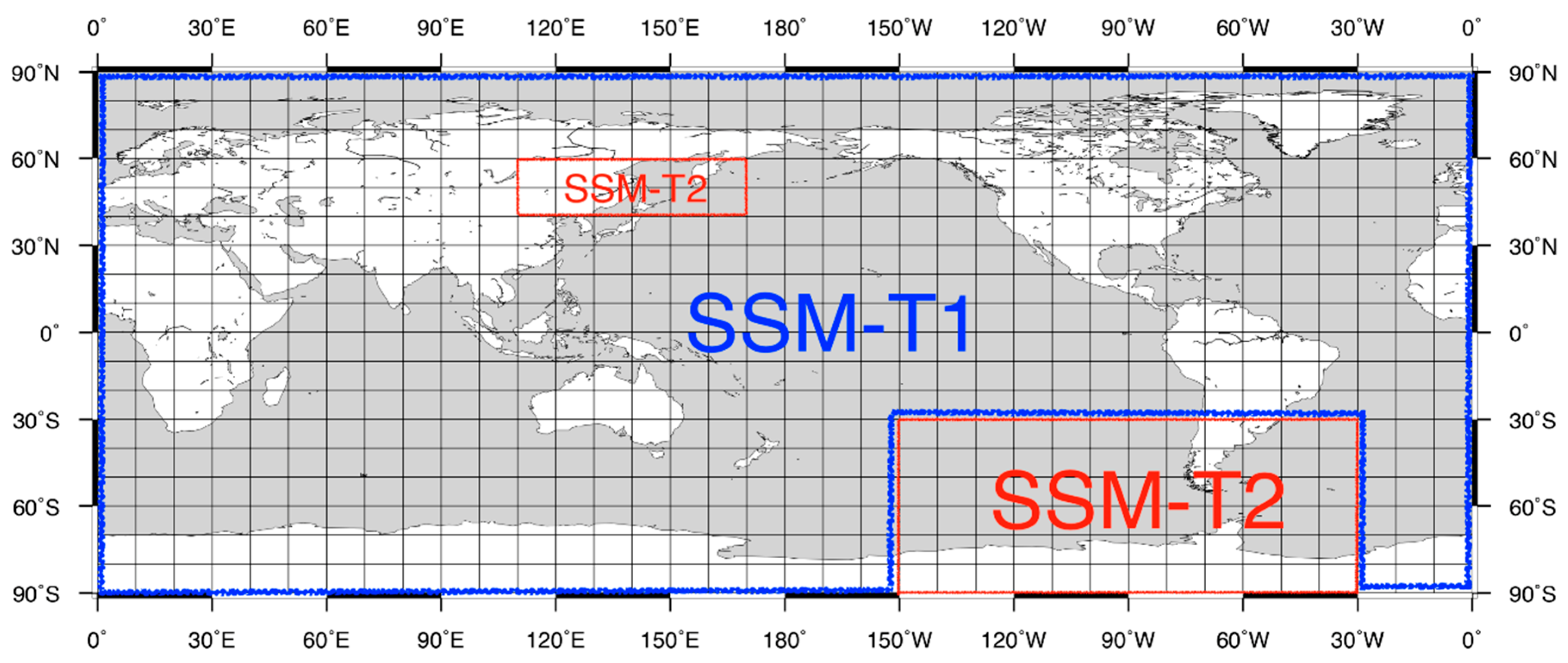
As the TECM-GRID is a discrete model based on 5183 grid points, it can effectively avoid the influence of ionospheric anomalies that are only related to locations, such as EIA. However, the approach of the TECM-GRID model cannot avoid time-related ionospheric anomalies, such as the MSNA phenomena. Therefore, the proposed TECM-GRID model does not use only one modelling function. Two different TEC empirical models, SSM-T1 and SSM-T2, are employed for grid points in different regions. SSM-T1, which was proposed in our previous study, exhibits good fit and forecasting precision on testing stations at the middle and low latitudes, but is unsuitable for stations in the MSNA area [33]. SSM-T1 can be used for single grid point modelling in areas other than MSNA. For grid points in the MSNA area, we proposed SSM-T2, as seen later in this paper. Note that the TECM-GRID model mainly considers the influence of the MSNA phenomenon. Relevant studies [24,26] show that the main occurrence areas of MSNA are (40–60°N, 110–170°E) and (30–90°S, 30–150° W), which correspond to eastern Asia (northeast China and northern Japan) and the Weddell Sea region near the Antarctic Peninsula, respectively. Therefore, in the MSNA region (40–60°N, 110–170°E) and (30–90°S, 30–150°W), the TECM-GRID adopts the SSM-T2 modelling method; in other regions of the world, the TECM-GRID adopts the SSM-T1 modelling method (Figure 1).
2.1. SSM-T1 Model
Over a single grid point, the variations of TEC are independent of the geographic or geomagnetic latitudes and longitudes. Thus, the variation characteristics mainly include the diurnal, seasonal and solar variations of TEC. Then, the single grid point TEC empirical model can be expressed in the form of multiplying three components [33]:
represents the diurnal variation component, represents the seasonal variation component and represents the variation that is dependent on solar activity. SSM-T1 is a function of day of year (DOY), local time (LT) and solar activity parameters.
The diurnal variation curve of TEC shows periodicity. Generally, the TEC value is the smallest at night, gradually increases after sunrise, and reaches the maximum around noon. In the SSM-T1 model, the TEC diurnal component consists of four harmonics and four correction coefficients:
The seasonal variation of TEC is also periodic. Similar to the TEC diurnal variation component model, the seasonal variation component of TEC takes the form of four harmonics (describing 1 year, half year, 1/3 year and 1/4 year periods, respectively) and four correction coefficients:
Unlike the existing empirical models [10,17,18,34], the SSM-T1 model takes F10.7p as the solar activity parameter. F10.7p is the average of F10.7 and F10.7A (the 81-day sliding average of F10.7). Compared with F10.7, a better linear relationship exists between F10.7p and Extreme Ultraviolet (EUV) [35,36,37], which can better reflect the intensity of solar activity. SSM-T1 regards the relationship between TEC and solar activity as linear, which can be described as:
In Equations (2)–(4), , , , , and are the 18 coefficients to be estimated, which are fitted by the non-linear least squares method.
2.2. SSM-T2 Model
Through the fitting test and model comparison, the SSM-T1 model is found unsuitable for stations in the MSNA area [33]. For grid points in the MSNA area, a new TEC empirical model SSM-T2 is proposed here. This model is based on SSM-T1. The diurnal component of SSM-T1 was modified and the MSNA correction term was added. The SSM-T2 model is still expressed in the form of multiplying three components:
represents the TEC diurnal variation component, represents the TEC seasonal variation component and represents the variation that is dependent on solar activity. SSM-T2 is also a function of DOY, LT and solar activity parameters.
Unlike the SSM-T1 model, the TEC diurnal variation component in SSM-T2 consists of two parts: the normal TEC diurnal variation characteristic (which is described by a combination of four harmonics and four correction coefficients) and the MSNA correction term. The specific expressions are as follows:
LT is the local time and , , , are the 17 coefficients to be estimated, which are fitted by the non-linear least squares method.
Considering that MSNA occurs in summer, the diurnal variation of TEC is exactly the opposite of that in winter, so . In Formula (7), the cosine function is used to locate the time period that must be corrected; then, the daily variation characteristics of MSNA are corrected by the cosine function .
The components of and in the SSM-T2 model are the same as those in the SSM-T1 model. In total, 27 coefficients are used for SSM-T2, which are fitted by the non-linear least squares method.
3. Model Results and Testing
The CODE GIMs TEC sequences of each grid point from 1 January 1999 to 30 June 2015 were taken as the modelling data set. Since its publication in 1998, the number, start time and epoch interval of GIMs in the Ionosphere Exchange format (IONEX) file have changed three times. They are: (1) before DOY (Day of Year) of 306 in 2002, for which 12 GIMs were generated every day from 01:00 to 23:00 with an interval of 2 h; (2) from DOY of 307 in 2002 to DOY of 291 in 2014, for which 13 GIMs were generated every day from 00:00 to 24:00 with an interval of 2 h; and (3) from DOY of 292 in 2014 to now, for which 25 GIMs are generated every day from 00:00 to 24:00 with an interval of 1 h. To unify the modelling dataset, GIMs TEC data were resampled with an interval of 2 h after DOY of 292 in 2014. Therefore, the time interval for all modelling datasets was 2 h. In addition, with the increasing number of IGS stations, the accuracy of CODE TEC data also improved. Note that the accuracies of GIMs TEC data with long time series differ in time scale, which affects the overall accuracy of the model. However, in the empirical model research, the longer the duration of modelling data (at least the longest time period should be covered), the more accurately the change characteristics of research objectives can be described. Considering the above two factors, the temporal inconsistency of accuracy was disregarded in this paper, as well as select long time modelling data of about 17 years, spanning 1.5 solar activity cycles. Furthermore, global TEC data were selected under geomagnetic conditions. Following the example of previous studies [33,38,39,40], GIMs TEC data for which the Ap index exceed 30.0 were not considered for modelling.
When the modelling data sets were applied to the corresponding SSM-T1 and SSM-T2 models, the fitting results of the undetermined coefficients as well as the covariance matrices were obtained by using the non-linear least squares method. Then, the standard deviations of the coefficients derived from the square roots of the diagonal elements of the covariance matrices were adopted to calculate the 95% confidence intervals of individual coefficients (Jakowski et al., 2011). As the TECM-GRID model contained 5183 sections, the number of model coefficients was large. The fitting results of the undetermined coefficients are not listed.
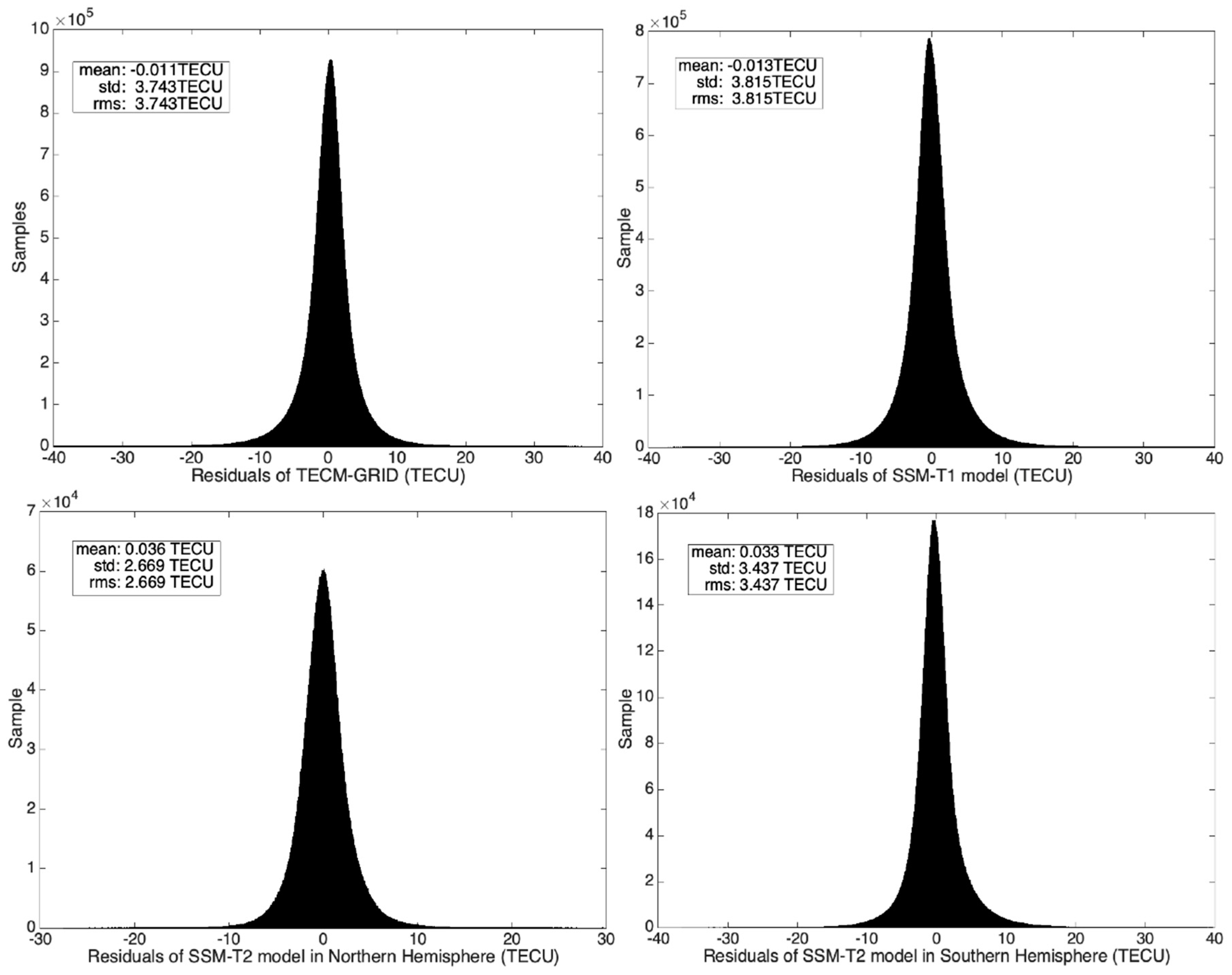
The model residuals of TECM-GRID as well as the sub-models of SSM-T1 and SSM-T2 (in the Southern and Northern Hemispheres) are shown in Figure 2. The model residuals showed a normal distribution, and most of the residuals were concentrated within ±5 TECU (Figure 2). The mean residual of TECM-GRID model was −0.011 TECU, with a root mean square error of 3.743 TECU and a standard deviation of 3.743 TECU. The TECM-GRID model was compared with the similar NTCM-GL model [17,41]. The mean residual of the NTCM-GL model was 0.3 TECU, the root mean square error of the residual was 7.516 TECU and the standard deviation of the residual was 7.5 TECU.
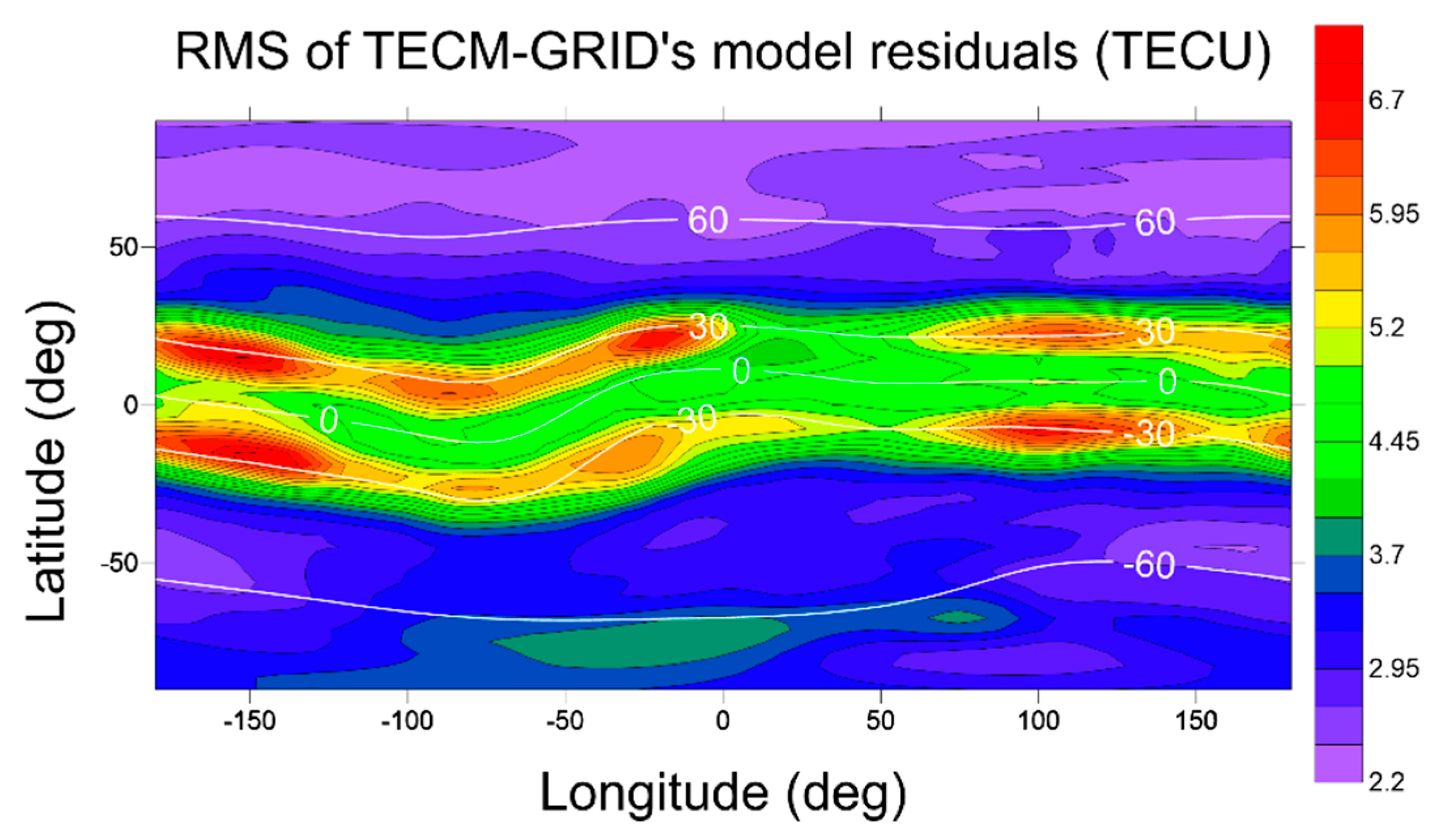
Then, we synthesized the model residuals and formed the contour map of the RMS value of model residuals globally, as shown in Figure 3. The model residuals of TECM-GRID were the smallest in the polar region and reached the maximum near 30 degrees offsetting north and south of the modified dip magnetic equator (Figure 3). The distribution characteristics of the RMS values of model residuals were consistent with those of global TEC values. The global distribution of TEC can be described as follows: with the increasing trend of solar radiation from the poles to the equator, TEC also shows an increasing trend from the poles to the equator, which is the smallest at both poles and the largest at low latitudes. In addition, because of the ‘fountain effect’, the TEC maximum is distributed on both sides of the modified dip magnetic equator. The magnitude of model residuals is positively correlated with the magnitude of model data. The bigger the TEC value in the modelling data, the bigger the model residual.
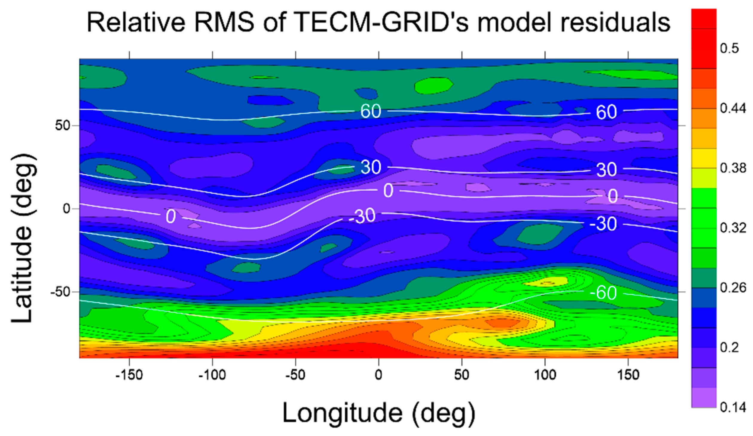
According to the above analysis, the best or worst fitting regions of the TECM-GRID model were not easily discovered by using model residuals. Accordingly, the relative RMS values of the model residuals were calculated. Here, the relative RMS was the ratio of the RMS value of the model residuals to the average value of the model dataset at each grid point, expressed as a percentage. Relative RMS value can effectively describe the fitting degree of the proposed model to the modelling dataset. Figure 4 shows the contours of the relative RMS values of the model residuals. The fitting ability of the TECM-GRID model for the modelling data was optimal near the modified dip magnetic equator, and the relative RMS value was about 15% (Figure 4). Such ability was at its worst in polar regions, especially in Antarctica, where the relative RMS value is as high as 50%. The main reasons for the poor performance of the TECM-GRID model in polar regions are as follows: (1) due to the existence of polar day and night, the regularity of TEC variations in polar regions is very poor, and accurately modelling it is difficult. Moreover, the variations of TEC differ in polar day and night. In further research, modelling polar day and night separately may be one of the feasible schemes to improve the accuracy of TEC empirical models in poles. Adding an index of geomagnetic activity to the sub-models in poles may be another feasible scheme. (2) Aside from depending on solar radiation, the ionization process of the polar ionosphere is also affected by particle deposition and Joule heating. This part of the radiation factor is challenging to model and is not involved in the current model. (3) Near Antarctica, the SSM-T2 model does not correct MSNA adequately. Time of MSNA occurrence is not limited to the local summer. Lin et al. [28] found that near the Antarctic Peninsula, MSNA may occur in January, February, October, November and December. The MSNA correction term in SSM-T2 does not involve the uncertainty of months when MSNA occurred, but roughly describes the change characteristics of MSNA in general, which may not be corrected in detail and adequately. Therefore, investigations on how to build MSNA correction terms by season or even by month are possible solutions for improving the accuracy of the SSM-T2 model for the MSNA area.
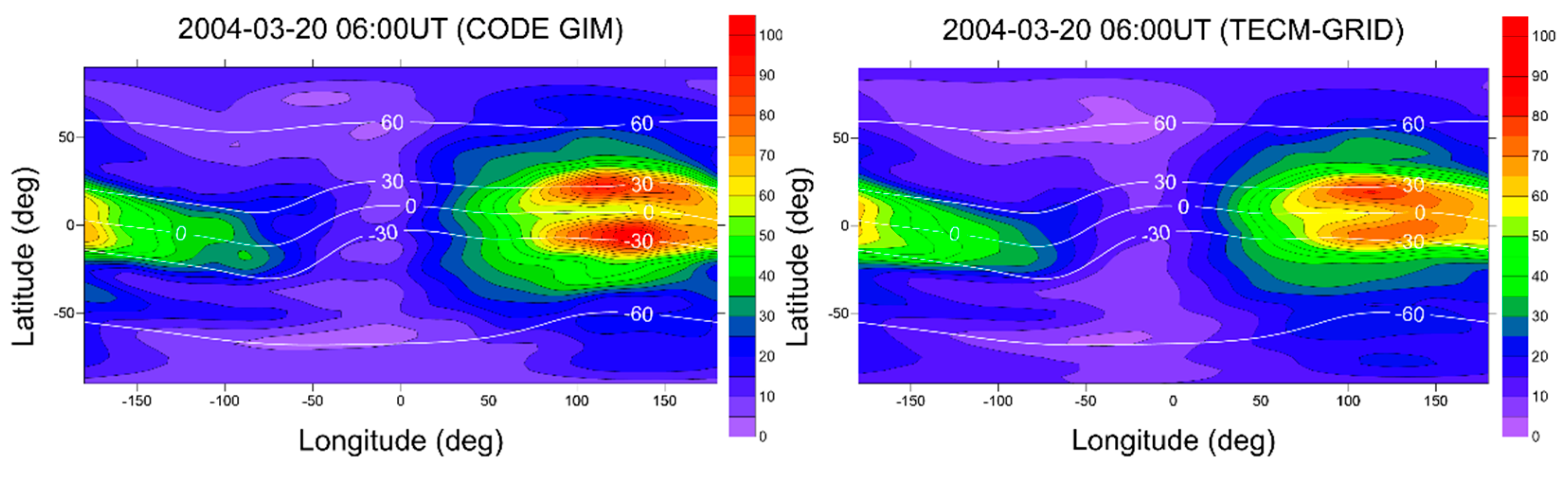
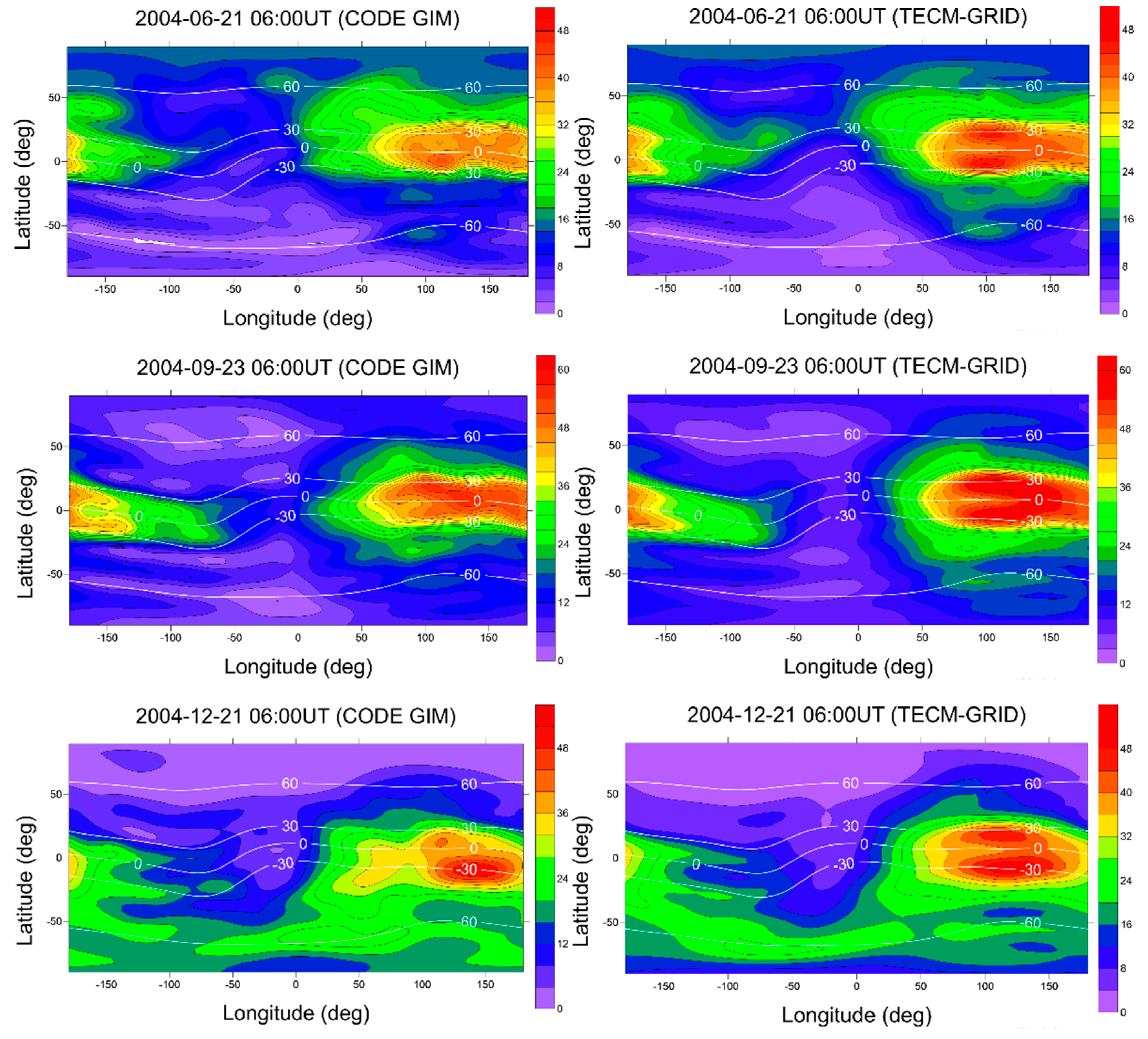
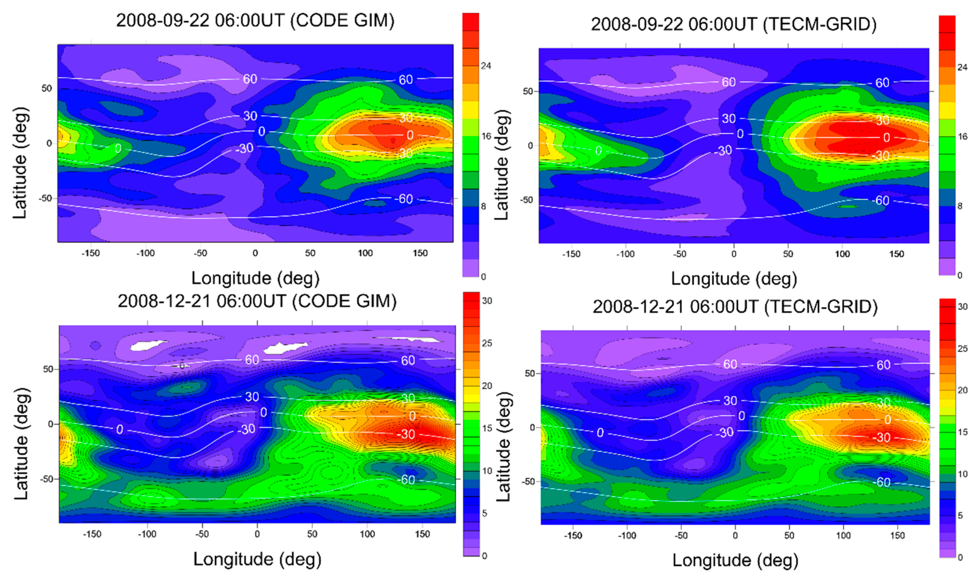
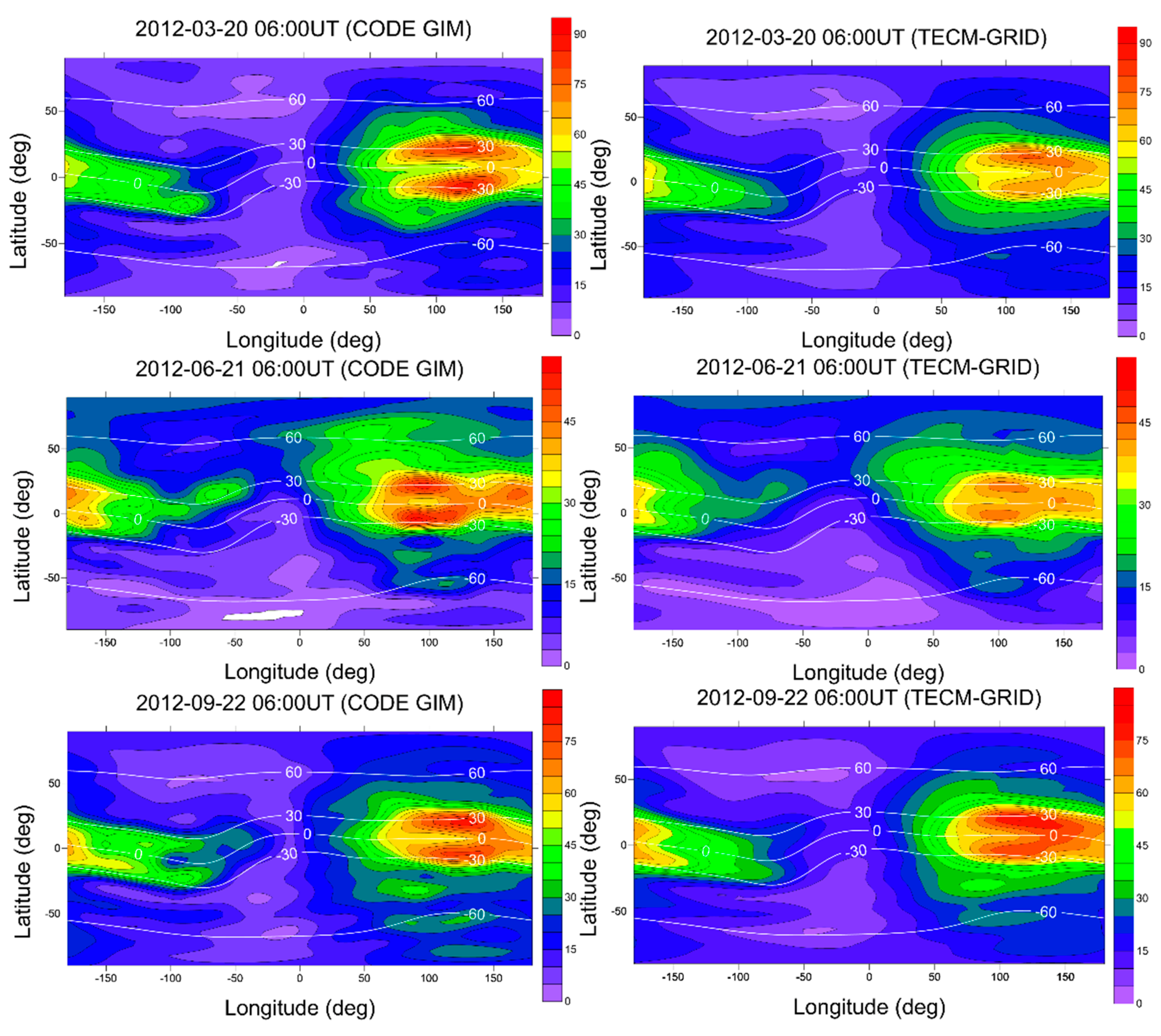
The fitting ability of the TECM-GRID model to CODE GIMs was tested for different solar activities and different seasons. Taking 2004, 2008 and 2012 as examples, the spring equinox, summer solstice, autumn equinox and winter solstice were selected as test days, and 6:00 UT was chosen as the test time. Figure 5, Figure 6 and Figure 7 show the comparison results of CODE GIMs and TECM-GRID models in 2004, 2008 and 2012, respectively. From these three Figures, we can see that: (1) both CODE GIMs and TECM-GRID reflect the EIA characteristics of TEC, and reflect the typical seasonal variation characteristics of EIA [42,43,44,45,46]. During the spring equinox (March 20) and autumn equinox (22 or 23 September), EIA’s double humps are symmetrical to the north and south of the modified dip magnetic equator; in the summer solstice (21 June) and the winter solstice (21 December), EIA shows asymmetry to the north and south hemisphere of the modified dip magnetic equator, and leans to the summer hemisphere. That is, EIA leans to the north hemisphere at the summer solstice and the south hemisphere at the winter solstice. (2) On 20 March 2004, 20 March and 21 June 2012, TECM-GRID underestimated the EIA peak plotted by CODE GIMs for the corresponding time. In other test days, however, the TECM-GRID model and CODE GIMs were generally consistent. (3) On 21 December 2004, 21 December 2008 and 21 December 2012, both CODE GIMs and TECM-GRID were able to describe MSNA phenomena. On 21 December 2012 and 21 December 2008, the phenomena of MSNA described by CODE GIMs and TECM-GRID were identical, while the counterpart for 21 December 2004 slightly differed. Table 1 gives the statistical results of the difference between TECM-GRID model and CODE GIM TEC, covering the global scope, the EIA region, MSNA region in the northern hemisphere and the southern hemisphere, respectively. Considering that the test time was selected at 06:00 UT, we chose (20°S~20°N; 50°E~180°E) as the range of EIA. From Table 1, we can see that: (1) RMS values of difference between CODE GIM and TECM-GRID in the global area were positively correlated with the solar activity parameter (F10.7), which ranged from 1.35 to 4.15 TECU. (2) The relative RMS values of difference in the global area were around 20%, which has no obvious correlation with solar activities. (3) The relative RMS values of difference in MSNA were larger in southern hemisphere than that in northern hemisphere. (4) The relative RMS values of difference in the EIA area ranged from 10.78% to 19.55%, with a mean value of 15.06%.
4. Model Validation and Comparison
Considering that the modelling period was from 1 January 1999 to 30 June 2015, we chose a time other than the modelling time to validate the TECM-GRID model. The selected test times were 06:00 UT on 1 February, 1 April, 1 June, 1 August, 1 October and 1 December 2016. The NTCM-GL model was selected for comparison. The reason for choosing NCTM-GL is that both of NTCM-GL and TECM-GRID were built by using CODE GIMs TEC and least squares fitting technique. They used the same reference dataset and the same technique for fitting. Then, TECM-GRID and NTCM-GL were compared with CODE GIMs to evaluate their performance.
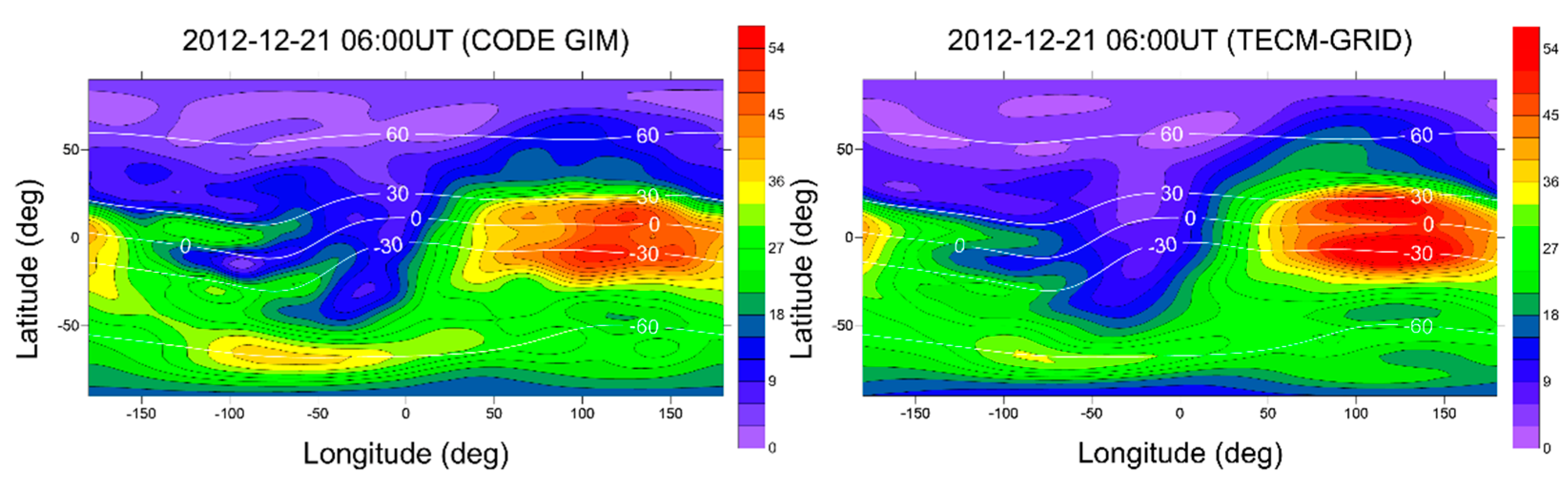
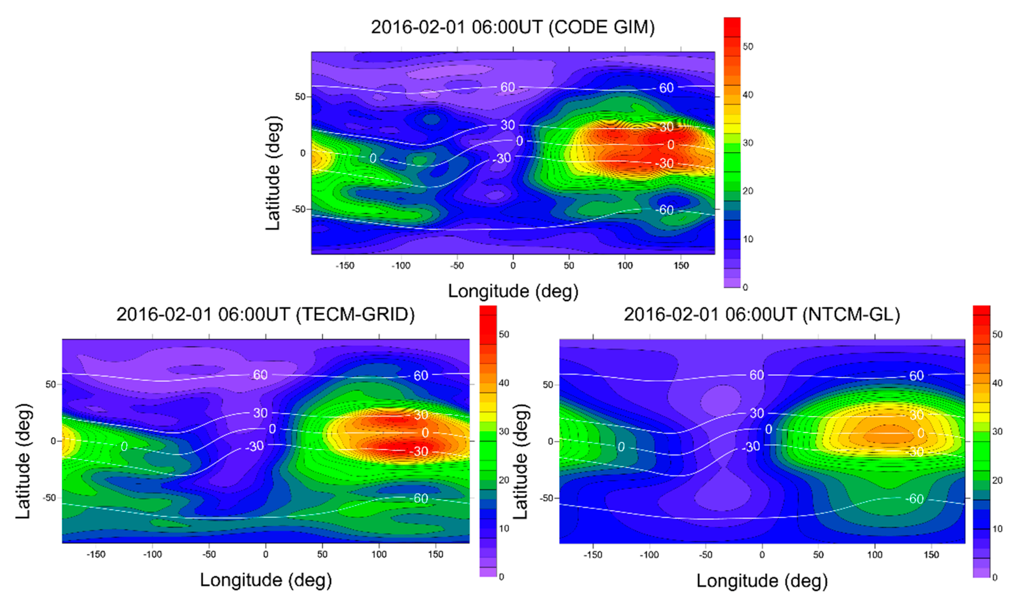
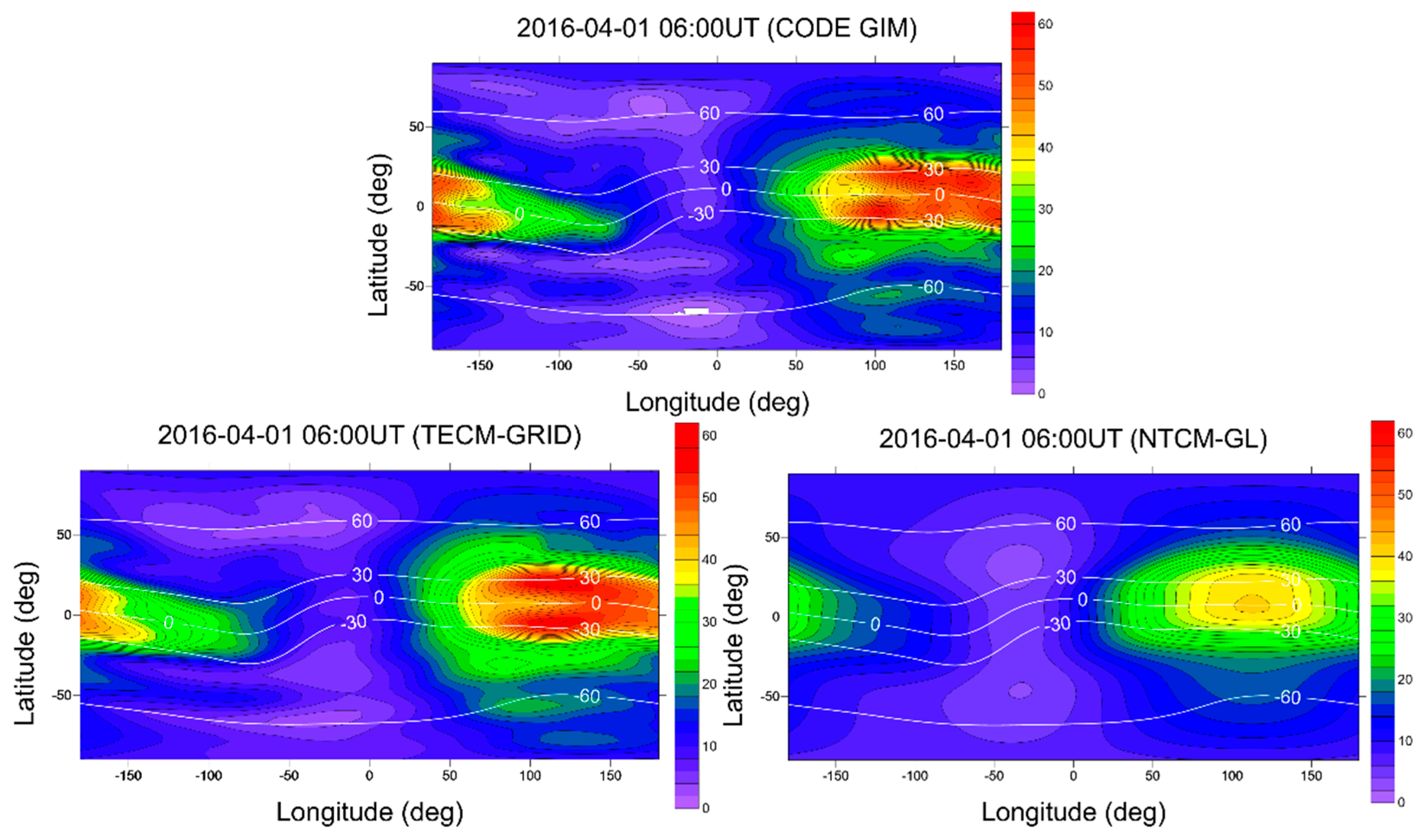
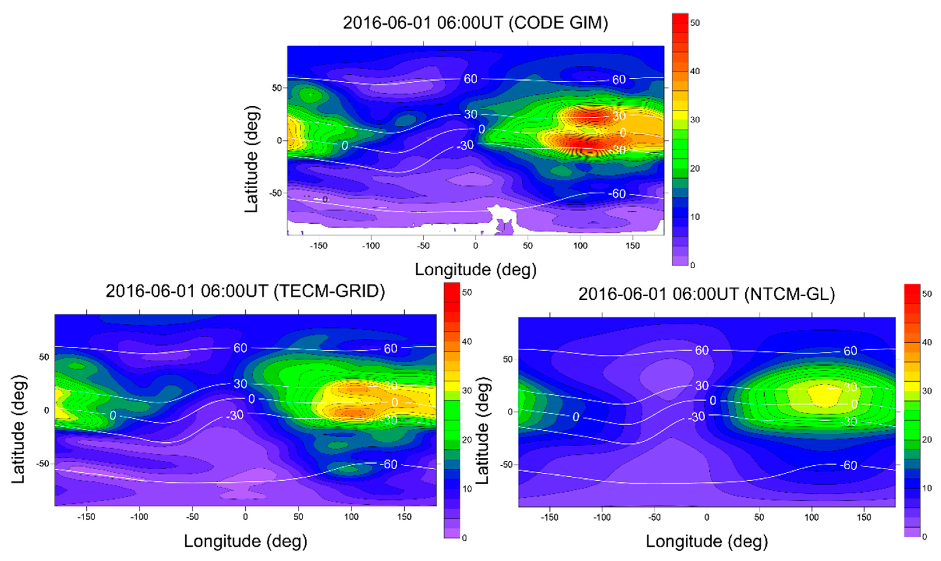
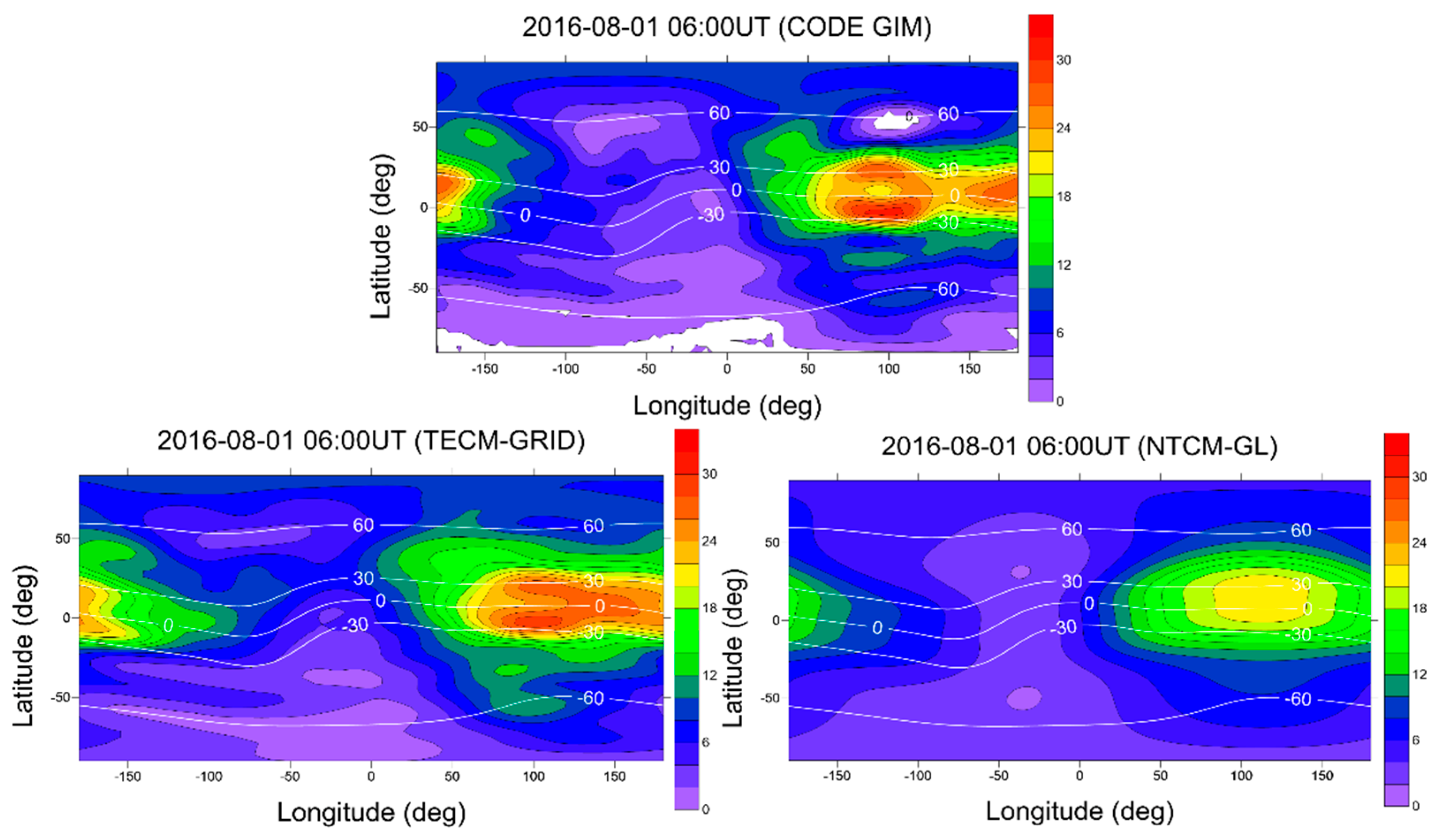
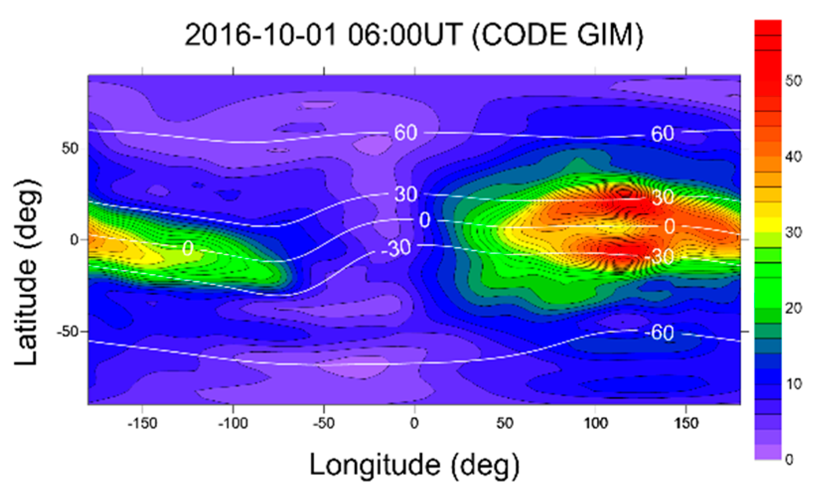
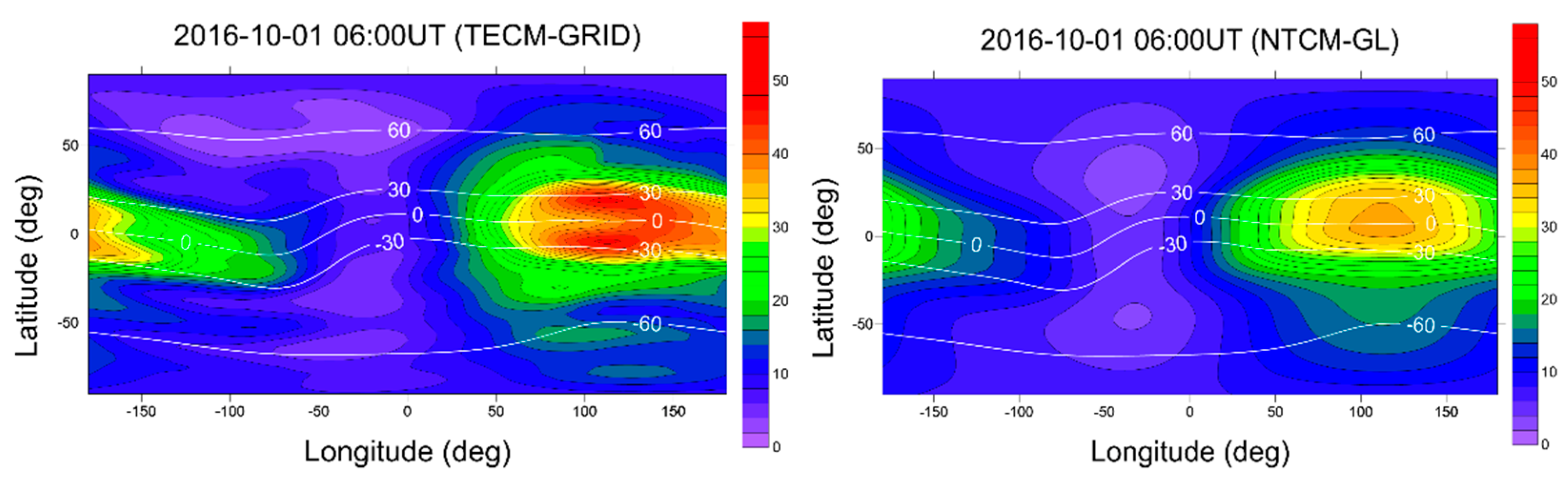
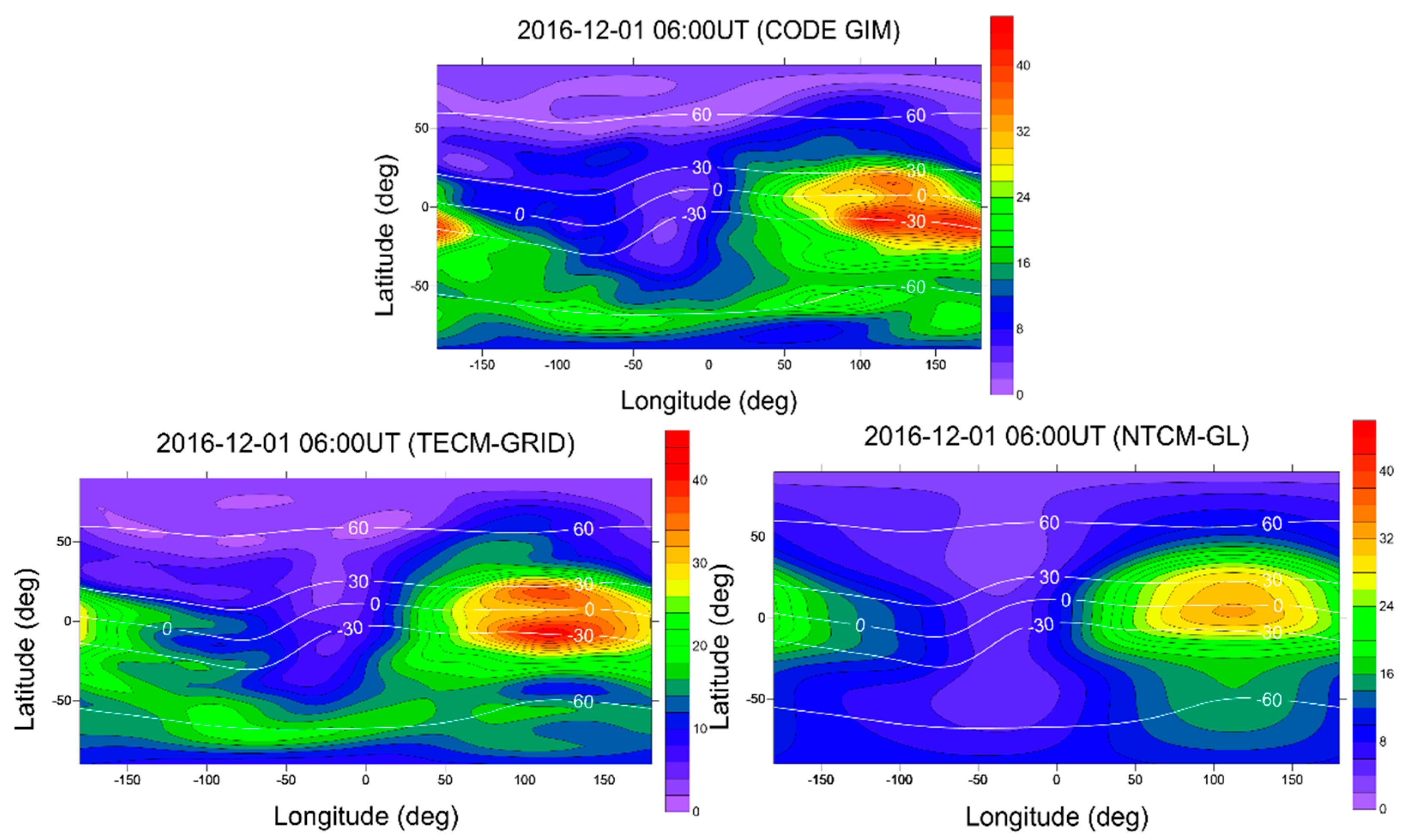
Figure 8, Figure 9, Figure 10, Figure 11, Figure 12 and Figure 13 depict the TEC maps derived from the TECM-GRID model, NTCM-GL model and CODE GIMs at 06:00 UT on 1 February, 1 April, 1 June, 1 August, 1 October and 1 December 2016, respectively. Note that the global ionospheric TEC maps drawn by CODE GIMs show blank areas in some areas, which are negative values when CODE GIMs are interpolated. These results were due to the fact that few or no stations were present in the region, and the ionospheric puncture points could not be effectively covered [47].
Figure 8, Figure 9, Figure 10, Figure 11, Figure 12 and Figure 13 indicate that: (1) the TECM-GRID model and CODE GIMs can describe EIA phenomena, for which the results of the EIA described by the TECM-GRID model were the closest to those of CODE GIMs. The global TEC map calculated by the NTCM-GL model at all test times had only one peak over the equator, which cannot describe EIA phenomena. (2) At 06:00 UT on 1 December 2016, the TECM-GRID model described MSNA phenomena very well, and the results were the closest to those of CODE GIMs. The results of NTCM-GL model did not show any MSNA characteristics. (3) Compared with the NTCM-GL model, the TECM-GRID model described more details of TEC distribution in the ionosphere, especially at night.
For the selected testing time, CODE GIMs were subtracted from TECM-GRID model and NTCM-GL model. Then, the RMS of the difference was calculated. Results are shown in Table 2. The RMS of the differences between CODE GIMs and TECM-GRID were always the smaller on testing days (Table 2).
An important concern of this model is the MSNA, and the EIA can also be reproduced in this model. In this part, we focus on the analysis of MSNA and EIA, as well as the global scope over a longer extrapolation period (2016–2018). The spring equinox, summer solstice, autumn equinox and winter solstice in 2016, 2017 and 2018 were selected as test days. Then the TECM-GRID and NTCM-GL model were compared with CODE GIMs, and the differences between them were computed and analyzed, as shown in Table 3. From Table 3, we can see that the TECM-GRID model is superior to the NTCM-GL model in fitting CODE GIM in extrapolation time, whether in global or regional scales (EIA area and MSNA area in the northern and southern hemispheres). This indicated the advantage of discrete modeling proposed in this paper, especially in the expression of ionospheric anomalies.
5. Summary and Discussion
To deal with the uneven accuracy of modelling TEC data and the regional differences in ionospheric TEC variation characteristics, a grid-based modelling pattern (which is essentially a set of models) was proposed for the first time through this paper. According to the location of grid points, we chose two different sub-models. The SSM-T2 model was selected as the sub-model in the MSNA region, and SSM-T1 model was selected as the sub-model in other regions. Finally, the fitting results of the undetermined coefficients in the 95% confidence interval were obtained by using the non-linear least squares method. Then, the TECM-GRID model was analysed using the RMS value and relative RMS value of the residual distribution. This approach tested the fitting ability of the TECM-GRID model to the modelling data. Finally, the TECM-GRID model was validated and compared with NTCM-GL and CODE GIMs beyond the time of model establishment. The results showed that TECM-GRID could better describe the EIA and MSNA phenomena, and was in good agreement with CODE GIMs.
The TECM-GRID model was proposed based on the NTCM-GL model. Both models were built by using CODE GIMs TEC and the least squares fitting technique. The NTCM-GL model adopts overall modelling, while the TECM-GRID model adopts discrete modelling. These two modelling methods have their own advantages and disadvantages. The discrete modelling method can overcome the influence from the uneven accuracy of CODE GIM and is advantageous for describing some abnormal phenomena of the ionosphere. However, compared with the NTCM-GL model, discrete modelling has some disadvantages. For example, the TECM-GRID model contains 5183 grid points. Considering the space limitation of this paper, the determined coefficients on each grid point were not given, so its practicability is limited. In this respect, the NTCM-GL model has significant advantages. The NTCM-GL model is a concise, fast and friendly empirical model with only 12 coefficients. This model is very convenient to use and is operable, which can provide TEC data on different solar activities for global users.
Moreover, the TECM-GRID model only focuses on the most obvious anomaly, MSNA, because the TEC diurnal variability in the MSNA region is quite different or even contrary to that in other regions during night time in the summer. In fact, other anomalies are present in the ionosphere around the world, such as the NWA anomaly [48]. TEC winter anomalies occurred in the Arctic, North America, and Nordic regions of the Northern Hemisphere [49]. In addition, the ionospheric TEC showed asymmetry between the northern and southern hemispheres [50,51]; in the South and North Poles, the variation characteristics of the ionospheric TEC during polar day or night vary considerably from those of the ionospheric TEC in the middle and low latitudes. Therefore, according to the idea of the modelling pattern proposed in this paper, the SSM-GRID model has room for improvement. If all abnormal phenomena of the ionosphere are considered and modelled reasonably according to the location of grid points, then the accuracy of the model will be further improved.
Author Contributions
J.F. and Z.W. proposed the core concept of the study. H.B. designed and performed the experiments. Z.Z. developed a summary and wrote the paper.
Funding
This research was funded by National Natural Science Foundation of China (Grant Nos. 41804032 and 41774019), the Key Laboratory of Geospace Environment and Geodesy, the Ministry of Education, Wuhan University (17-01-11), State Key Laboratory of Geodesy and Earth’s Dynamics (Grant No. SKLGED2019-3-4-E) and project supported by the specialized research fund for state key laboratories.
Acknowledgments
We thank the IGS CODE analysis centre for GIMs TEC data. The authors thank three anonymous reviewers and editors for improving the quality of paper.
Conflicts of Interest
The authors declare no conflict of interest.
References
- Wu, X.; Hu, X.; Wang, G.; Zhong, H.; Tang, C. Evaluation of COMPASS ionospheric model in GNSS positioning. Adv Space Res 2013, 51, 959–968. [Google Scholar] [CrossRef]
- Zhang, Q.; Zhao, Q.L.; Zhang, H.P.; Hu, Z.G.; Wu, Y. Evaluation on the precision of Klobuchar model for BeiDou navigation satellite system. Geomat. Inf. Sci. Wuhan Univ. 2014, 39, 142–146. [Google Scholar]
- Bilitza, D.; Altadill, D.; Reinisch, B.; Galkin, I.; Shubin, V.; Truhlik, V. The International Reference Ionosphere: Model Update 2016. In Proceedings of the EGU General Assembly, Vienna, Austria, 17–22 Arpil 2016. [Google Scholar]
- Nava, B.; Coïsson, P.; Radicella, S.M. A new version of the NeQuick ionosphere electron density model. J. Atmos. Sol.-Terr. Phys. 2008, 70, 1856–1862. [Google Scholar] [CrossRef]
- Radicella, S.M.; Nava, B. NeQuick model: Origin and evolution. In Proceedings of the International Symposium on Antennas Propagation and Em Theory, Guangzhou, China, 29 November–2 December 2010; pp. 422–425. [Google Scholar]
- Mao, T.; Xing, W.W.; Liu, L.B. An EOF-based empirical model of TEC over Wuhan. Chin. J. Geophys. 2005, 48, 751–758. [Google Scholar] [CrossRef]
- Huang, Z.; Yuan, H. Ionospheric single-station TEC short-term forecast using RBF neural network. Radio Sci. 2014, 49, 283–292. [Google Scholar] [CrossRef] [Green Version]
- Huang, Z.; Li, Q.B.; Yuan, H. Forecasting of ionospheric vertical TEC 1-h ahead using a genetic algorithm and neural network. Adv. Space Res. 2015, 55, 1775–1783. [Google Scholar] [CrossRef]
- Hajra, R.; Chakraborty, S.K.; Tsurutani, B.T.; Dasgupta, A.; Echer, E.; Brum, C.G.M.; Gonzalez, W.D.; Sobral, J.H.A. An empirical model of ionospheric total electron content (TEC) near the crest of the equatorial ionization anomaly (EIA). J. Space Weather Space Clim. 2016, 6, A29. [Google Scholar] [CrossRef] [Green Version]
- Jakowski, N. TEC Monitoring by Using Satellite Positioning Systems. In Modern Ionospheric Science; European Geophysical Society: Munich, Germany, 1996; pp. 371–390. [Google Scholar]
- Opperman, B.D.L.; Cilliers, P.J.; Mckinnell, L.A.; Haggard, R. Development of a regional GPS-based ionospheric TEC model for South Africa. Adv Space Res. 2007, 39, 808–815. [Google Scholar] [CrossRef]
- Mao, T.; Wan, W.X.; Yue, X.N.; Sun, L.F.; Zhao, B.Q.; Guo, J.P. An empirical orthogonal function model of total electron content over China. Radio Sci. 2008, 43, 1–12. [Google Scholar] [CrossRef]
- Bouya, Z.; Terkildsen, M.; Neudegg, D. Regional GPS-based ionospheric TEC model over Australia using Spherical Cap Harmonic Analysis. In Proceedings of the 38th COSPAR Scientific Assembly, Bremen Germany, 18–15 July 2010; p. 4. [Google Scholar]
- Habarulema, J.B.; McKinnell, L.A.; Opperman, B.D.L. TEC measurements and modelling over Southern Africa during magnetic storms; a comparative analysis. J. Atmos. Sol.-Terr. Phys. 2010, 72, 509–520. [Google Scholar] [CrossRef]
- Habarulema, J.B.; McKinnell, L.A.; Opperman, B.D.L. Regional GPS TEC modeling; Attempted spatial and temporal extrapolation of TEC using neural networks. J. Geophys. Res.-Space 2011, 116, A04314. [Google Scholar] [CrossRef]
- Chen, Z.; Zhang, S.; Coster, A.J.; Fang, G. EOF analysis and modeling of GPS TEC climatology over North America. J. Geophys. Res. Space Phys. 2015, 120, 3118–3129. [Google Scholar] [CrossRef] [Green Version]
- Jakowski, N.; Hoque, M.M.; Mayer, C. A new global TEC model for estimating transionospheric radio wave propagation errors. J Geod. 2011, 85, 965–974. [Google Scholar] [CrossRef]
- Mukhtarov, P.; Pancheva, D.; Andonov, B.; Pashova, L. Global TEC maps based on GNSS data: 1. Empirical background TEC model. J. Geophys. Res. Space Phys. 2013, 118, 4594–4608. [Google Scholar] [CrossRef] [Green Version]
- Mukhtarov, P.; Pancheva, D.; Andonov, B.; Pashova, L. Global TEC maps based on GNNS data: 2. Model evaluation. J. Geophys. Res. Space Phys. 2013, 118, 4609–4617. [Google Scholar] [CrossRef] [Green Version]
- Andonov, B. Global empirical background TEC model: Long-term prediction model. In Proceedings of the EGU General Assembly Conference, Vienna, Austria, 7–12 April 2013. [Google Scholar]
- Mukhtarov, P.; Pancheva, D.; Andonov, B. Hybrid model for long-term prediction of the ionospheric global TEC. J. Atmos. Sol.-Terr. Phys. 2014, 119, 1–10. [Google Scholar] [CrossRef]
- Ercha, A.; Zhang, D.; Ridley, A.J.; Xiao, Z.; Hao, Y. A global model: Empirical orthogonal function analysis of total electron content 1999–2009 data. J. Geophys. Res. Space Phys. 2012, 117, A03328. [Google Scholar]
- Wan, W.X.; Ding, F.; Ren, Z.P.; Zhang, M.L.; Liu, L.B.; Ning, B.Q. Modeling the global ionospheric total electron content with empirical orthogonal function analysis. Sci. China Technol. Sci. 2012, 55, 1161–1168. [Google Scholar] [CrossRef]
- Lin, C.H.; Liu, J.Y.; Cheng, C.Z.; Chen, C.H.; Liu, C.H.; Wang, W.; Burns, A.G.; Lei, J. Three-dimensional ionospheric electron density structure of the Weddell Sea Anomaly. J. Geophys. Res.-Space 2009, 114. [Google Scholar] [CrossRef] [Green Version]
- Thampi, S.V.; Lin, C.; Liu, H.X.; Yamamoto, M. First tomographic observations of the Midlatitude Summer Nighttime Anomaly over Japan. J. Geophys. Res.-Space 2009, 114. [Google Scholar] [CrossRef] [Green Version]
- Horvath, I.; Lovell, B.C. An investigation of the northern hemisphere midlatitude nighttime plasma density enhancements and their relations to the midlatitude nighttime trough during summer. J. Geophys. Res.-Space 2009, 114. [Google Scholar] [CrossRef] [Green Version]
- Liu, H.; Thampi, S.V.; Yamamoto, M. Phase reversal of the diurnal cycle in the midlatitude ionosphere. J. Geophys. Res. 2010, 115, 81–85. [Google Scholar] [CrossRef]
- Lin, C.H.; Liu, C.H.; Liu, J.Y.; Chen, C.H.; Burns, A.G.; Wang, W. Midlatitude summer nighttime anomaly of the ionospheric electron density observed by FORMOSAT-3/COSMIC. J. Geophys. Res. 2010, 115. [Google Scholar] [CrossRef]
- Klobuchar, J.A. Ionospheric time-delay algorithm for single-frequency GPS users. IEEE Trans. Aerosp. Electron. Syst. 1987, AES-23, 325–331. [Google Scholar] [CrossRef]
- Pavel, N.; Tomislav, K. Performance analysis of empirical ionosphere models by comparison with CODE vertical TEC maps. In Mitigation of Ionospheric Threats to GNSS: An Appraisal of the Scientific and Technological Outputs of the TRANSMIT Project; IntechOpen: London, UK, 2014. [Google Scholar]
- Feng, J.; Wang, Z.; Jiang, W.; Zhao, Z.; Zhang, B. A single-station empirical model for TEC over the Antarctic Peninsula using GPS-TEC data. Radio Sci. 2017, 52. [Google Scholar] [CrossRef]
- Venkatesh, K.; Fagundes, P.R.; Seemala, G.K.; Jesus, R.D.; Abreu, A.J.D.; Pillat, V.G. On the performance of the IRI-2012 and NeQuick2 models during the increasing phase of the unusual 24th solar cycle in the Brazilian equatorial and low latitude sectors. J. Geophys. Res. Space Phys. 2014, 119, 5087–5105. [Google Scholar] [CrossRef]
- Zhao, Z.Z.; Feng, J.D.; Han, B.M.; wang, Z.T. A single-station empirical TEC model based on long-time recorded GPS data for estimating ionospheric delay. J. Space Weather Space Clim. 2018, 8, 14. [Google Scholar] [CrossRef]
- Jakowski, N.; Sardon, E.; Schluter, S. GPS-based TEC observations in comparison with IRI95 and the European TEC model NTCM2. In Proceedings of the IRI 1997 Symposium: New Developments in Ionospheric Modelling and Prediction, Advances in Space Research, Kuhlungsborn, Germany, 27–30 May 1997; Volume 22, pp. 803–806. [Google Scholar]
- Richards, P.G.; Fennelly, J.A.; Torr, D.G. Euvac: A solar Euv Flux Model for aeronomic calculations. J. Geophys. Res.-Space 1994, 99, 8981–8992. [Google Scholar] [CrossRef]
- Bilitza, D. The importance of EUV indices for the international reference ionosphere. Phys. Chem. Earth Pt C 2000, 25, 515–521. [Google Scholar] [CrossRef]
- Liu, L.B.; Wan, W.X.; Ning, B.Q.; Pirog, O.M.; Kurkin, V.I. Solar activity variations of the ionospheric peak electron density. J. Geophys. Res.-Space 2006, 111. [Google Scholar] [CrossRef] [Green Version]
- Hedin, A.E. Correlations between thermospheric density and temperature, solar EUV flux, and 10.7-cm flux variations. J. Geophys. Res. 1984, 89, 9828. [Google Scholar] [CrossRef]
- Feng, J.; Wang, Z.; Jiang, W.; Zhao, Z.; Zhang, B. A new regional total electron content empirical model in northeast China. Adv. Space Res. 2016, 58, 1155–1167. [Google Scholar] [CrossRef]
- Feng, J.; Jiang, W.; Wang, Z.; Zhao, Z.; Nie, L. Regional TEC model under quiet geomagnetic conditions and low-to-moderate solar activity based on CODE GIMs. J. Atmos. Sol.-Terr. Phys. 2017, 161, 88–97. [Google Scholar] [CrossRef]
- Jakowski, N.; Mayer, C.; Hoque, M.M.; Wilken, V. Total electron content models and their use in ionosphere monitoring. Radio Sci. 2011, 46, RS0D18. [Google Scholar] [CrossRef]
- Vila, P. Intertropical F 2 Ionization During June and July 1966. Radio Sci. 1971, 6, 689–697. [Google Scholar] [CrossRef]
- Aydoǧdu, M. North-south asymmetry in the ionospheric equatorial anomaly in the African and the West Asian regions produced by asymmetrical thermospheric winds. J. Atmos. Terr. Phys. 1988, 50, 623–627. [Google Scholar] [CrossRef]
- Zhao, B.; Wan, W.; Liu, L. Response of equatorial anomaly to the October-November 2003 superstorm. Ann. Geophs. 2005, 23, 693–706. [Google Scholar] [CrossRef]
- Huang, L.; Huang, J.; Wang, J.; Jiang, Y.; Deng, B.; Zhao, K.; Lin, G. Analysis of the north–south asymmetry of the equatorial ionization anomaly around 110°E longitude. J. Atmos. Sol.-Terr. Phys. 2013, 102, 354–361. [Google Scholar] [CrossRef]
- Xiong, C.; Lühr, H. Nonmigrating tidal signatures in the magnitude and the inter-hemispheric asymmetry of the equatorial ionization anomaly. Ann. Geophys. 2013, 31, 1115–1130. [Google Scholar] [CrossRef] [Green Version]
- Wang, C.; Wang, J.X.; Duan, B.B. Global ionospheric model with international reference ionosphere constraint. Geomat. Inf. Sci. Wuhan Univ. 2014, 39, 1340–1346. [Google Scholar]
- Jakowski, N.; Hoque, M.M.; Kriegel, M.; Patidar, V. The persistence of the NWA effect during the low solar activity period 2007–2009. J. Geophys. Res. Space Phys. 2015, 120, 9148–9160. [Google Scholar] [CrossRef]
- Yu, T.; Wan, W.X.; Liu, L.B.; Tang, W.; Luan, X.L.; Yang, G.L. Using IGS data to analysis the global TEC annual and semiannual variation. Chin. J. Geophys. 2006, 49, 943–949. [Google Scholar] [CrossRef]
- Liu, L.; Zhao, B.; Wan, W.; Venkartraman, S.; Zhang, M.L.; Yue, X. Yearly variations of global plasma densities in the topside ionosphere at middle and low latitudes. J. Geophys. Res. Space Phys. 2007, 112. [Google Scholar] [CrossRef]
- Feng, J.D.; Jiang, W.P.; Wang, Z.T. Asymmetry of TEC between the southern and northern hemispheres based on IGS data. Geomat. Inf. Sci. Wuhan Univ. 2015, 40, 1354–1359. [Google Scholar]
Figure 1.
Geographic latitude and longitude range of the SSM-T1 and SSM-T2 for the TECM-GRID.

Figure 2.
Model Residual Distribution Histogram of TECM-GRID and sub-models (SSM-T1 and SSM-T2).

Figure 3.
RMS value of model residual for TECM-GRID. (Notes. The modified dip latitude is marked by a white line, henceforth.)
Figure 3.
RMS value of model residual for TECM-GRID. (Notes. The modified dip latitude is marked by a white line, henceforth.)

Figure 4.
Relative RMS values of model residuals for TECM-GRID.

Figure 5.
Comparison of CODE GIMs and TECM-GRID models (2004).


Figure 6.
Comparison of CODE GIMs and TECM-GRID models (2008).


Figure 7.
Comparison of CODE GIMs and TECM-GRID models (2012).


Figure 8.
Comparison of TECM-GRID and NTCM-GL with the CODE GIM (1 February 2016).

Figure 9.
Comparison of TECM-GRID and NTCM-GL with the CODE GIM (1 April 2016).

Figure 10.
Comparison of TECM-GRID and NTCM-GL with the CODE GIM (1 June 2016).

Figure 11.
Comparison of TECM-GRID and NTCM-GL with the CODE GIM (1 August 2016).

Figure 12.
Comparison of TECM-GRID and NTCM-GL with the CODE GIM (1 October 2016).


Figure 13.
Comparison of TECM-GRID and NTCM-GL with the CODE GIM (1 December 2016).


Table 1.
RMS and relative RMS statistics of difference between CODE GIM and TECM-GRID.
| Date (06:00UT) | F10.7 (sfu) | Global Area | MSNA in North | MSNA in South | EIA at 06:00 UT | ||||
|---|---|---|---|---|---|---|---|---|---|
| RMS | Relative RMS | RMS | Relative RMS | RMS | Relative RMS | RMS | Relative RMS | ||
| 20 March 2004 | 112.7 | 3.41 | 17.87% | 2.45 | 12.89% | 2.40 | 23.82% | 7.26 | 11.44% |
| 21 June 2004 | 119.6 | 3.13 | 22.56% | 2.93 | 16.82% | 1.18 | 31.79% | 7.68 | 19.55% |
| 23 September 2004 | 90.8 | 2.85 | 18.91% | 1.89 | 14.86% | 1.30 | 19.52% | 6.49 | 15.78% |
| 21 December 2004 | 97.7 | 3.02 | 19.66% | 1.79 | 19.22% | 3.22 | 18.23% | 6.56 | 18.56% |
| 20 March 2008 | 67.9 | 1.36 | 19.02% | 0.82 | 13.39% | 0.53 | 28.04% | 2.26 | 12.59% |
| 21 June 2008 | 67.0 | 1.35 | 20.67% | 1.20 | 16.67% | 0.75 | 39.68% | 2.63 | 13.65% |
| 22 September 2008 | 69.6 | 1.51 | 21.22% | 1.14 | 14.40% | 1.20 | 38.95% | 2.72 | 13.73% |
| 22 December 2008 | 65.5 | 1.52 | 17.87% | 0.67 | 14.85% | 1.98 | 21.96% | 2.36 | 10.78% |
| 20 March 2012 | 98.8 | 3.06 | 17.31% | 2.49 | 11.17% | 3.27 | 34.14% | 6.62 | 11.46% |
| 21 June 2012 | 100.9 | 2.96 | 19.18% | 2.87 | 15.88% | 1.20 | 30.53% | 6.86 | 19.37% |
| 22 September 2012 | 125.3 | 4.15 | 17.22% | 1.97 | 8.87% | 2.29 | 19.56% | 8.79 | 16.61% |
| 21 December 2012 | 110.9 | 3.24 | 16.85% | 1.55 | 14.06% | 5.63 | 21.63% | 7.58 | 17.23% |
Table 2.
RMS Statistics and Optimal Model Evaluation of difference between CODE GIM and TECM-GRID.
| Date | RMS (GIM—TECM-GRID) | RMS (GIM—NTCM-GL) |
|---|---|---|
| 1 February 2016 | 3.71 | 5.67 |
| 1 April 2016 | 2.62 | 6.19 |
| 1 June 2016 | 2.78 | 4.74 |
| 1 August 2016 | 2.46 | 4.06 |
| 1 October 2016 | 3.27 | 4.51 |
| 1 December 2016 | 2.76 | 5.53 |
Table 3.
RMS Statistics of difference between CODE GIM and models (TECM-GIRD and NTCM-GL).
| Date (06:00UT) | F10.7 (sfu) | RMS of Global(TECU) | Relative RMS of Global | RMS of MSNA in North | RMS of MSNA in South | RMS of EIAat 06:00UT | |||||
|---|---|---|---|---|---|---|---|---|---|---|---|
| C1 | C2 | C1 | C2 | C1 | C2 | C1 | C2 | C1 | C2 | ||
| 20 March 2016 | 86.9 | 2.55 | 5.48 | 17.15% | 36.92% | 1.28 | 3.77 | 1.27 | 3.02 | 4.23 | 9.88 |
| 21 June 2016 | 82.9 | 2.16 | 4.49 | 21.18% | 44.09% | 1.34 | 2.37 | 0.95 | 1.87 | 3.59 | 6.75 |
| 22 September 2016 | 85.7 | 2.42 | 3.62 | 19.75% | 29.62% | 1.21 | 4.91 | 1.25 | 2.28 | 3.71 | 5.11 |
| 21 December 2016 | 72.6 | 2.13 | 4.47 | 20.60% | 43.32% | 0.93 | 3.33 | 1.38 | 5.23 | 3.10 | 9.11 |
| 20 March 2017 | 72.1 | 2.17 | 3.23 | 21.35% | 31.74% | 1.16 | 4.85 | 0.84 | 1.70 | 2.29 | 5.40 |
| 21 June 2017 | 76.2 | 1.67 | 2.61 | 22.53% | 35.10% | 1.51 | 1.77 | 0.73 | 1.54 | 2.10 | 2.75 |
| 23 September 2017 | 81.7 | 1.92 | 3.68 | 18.82% | 36.17% | 1.37 | 6.01 | 1.07 | 2.08 | 3.44 | 4.44 |
| 22 December 2017 | 72.9 | 1.75 | 4.84 | 18.17% | 50.17% | 0.85 | 4.74 | 1.36 | 7.48 | 2.99 | 5.77 |
| 21 March 2018 | 68.8 | 1.62 | 3.87 | 19.55% | 42.12% | 1.22 | 5.04 | 1.07 | 2.42 | 2.62 | 6.16 |
| 21 June 2018 | 84.2 | 1.57 | 2.76 | 21.59% | 37.83% | 1.53 | 3.70 | 0.57 | 1.78 | 2.04 | 3.68 |
| 23 September 2018 | 68.9 | 1.51 | 3.08 | 18.01% | 36.82% | 1.28 | 4.34 | 0.83 | 2.34 | 2.69 | 4.46 |
| 22 December 2018 | 68.7 | 1.60 | 3.56 | 19.25% | 42.82% | 0.95 | 3.59 | 1.33 | 4.35 | 2.34 | 5.90 |
Notes. C1 = GIM − TECM-GRID; C2 = GIM − NTCM-GL Unit: TECU.
© 2019 by the authors. Licensee MDPI, Basel, Switzerland. This article is an open access article distributed under the terms and conditions of the Creative Commons Attribution (CC BY) license (http://creativecommons.org/licenses/by/4.0/).
Share and Cite
MDPI and ACS Style
Feng, J.; Han, B.; Zhao, Z.; Wang, Z. A New Global Total Electron Content Empirical Model. Remote Sens. 2019, 11, 706. https://0-doi-org.brum.beds.ac.uk/10.3390/rs11060706
AMA Style
Feng J, Han B, Zhao Z, Wang Z. A New Global Total Electron Content Empirical Model. Remote Sensing. 2019; 11(6):706. https://0-doi-org.brum.beds.ac.uk/10.3390/rs11060706
Chicago/Turabian StyleFeng, Jiandi, Baomin Han, Zhenzhen Zhao, and Zhengtao Wang. 2019. "A New Global Total Electron Content Empirical Model" Remote Sensing 11, no. 6: 706. https://0-doi-org.brum.beds.ac.uk/10.3390/rs11060706
Note that from the first issue of 2016, this journal uses article numbers instead of page numbers. See further details here.