Analyzing the Uncertainty of Estimating Forest Aboveground Biomass Using Optical Imagery and Spaceborne LiDAR


1
School of Geography and Tourism, Qufu Normal University, Rizhao 276800, China
2
National Satellite Meteorological Center, China Meteorological Administration, Beijing 100101, China
3
Institute of Geographical Science and Natural Resources Research, Chinese Academy of Sciences, Beijing 100101, China
*
Author to whom correspondence should be addressed.
Remote Sens. 2019, 11(6), 722; https://0-doi-org.brum.beds.ac.uk/10.3390/rs11060722
Submission received: 18 February 2019
/
Revised: 20 March 2019
/
Accepted: 22 March 2019
/
Published: 26 March 2019
(This article belongs to the Section Forest Remote Sensing)
Abstract
:Accurate estimation of forest aboveground biomass (AGB) is important for carbon accounting. Forest AGB estimation has been conducted with a variety of data sources and prediction methods, but many uncertainties still exist. In this study, six prediction methods, including Gaussian processes, stepwise linear regression, nonlinear regression using a logistic model, partial least squares regression, random forest, and support vector machines were used to estimate forest AGB in Jiangxi Province, China, by combining Geoscience Laser Altimeter System (GLAS) data, Moderate Resolution Imaging Spectroradiometer (MODIS) data, and field measurements. We compared the effect of three factors (prediction methods, sample sizes of field measurements, and cross-validation settings) on the predictive quality of the methods. The results showed that the prediction methods had the most considerable effect on the prediction quality. In most cases, random forest produced more accurate estimates than the other methods. The sample sizes had an obvious effect on accuracy, especially for the random forest model. The accuracy increased with increasing sample sizes. The random forest algorithm with a large number of field measurements, was the most precise (coefficient of determination (R2) = 0.73, root mean square error (RMSE) = 23.58 Mg/ha). Increasing the number of folds within the cross-validation settings improved the R2 values. However, no apparent change occurred in RMSE for different numbers of folds. Finally, the wall-to-wall forest AGB map over the study area was generated using the random forest model.

1. Introduction
Forest ecosystems play a pivotal role in the global carbon cycle, and the contribution of the forest to carbon cycle is often quantified by forest aboveground biomass (AGB) [1]. AGB has been identified as a biodiversity variable suitable for estimating ecosystem functions [2]. There is particular interest in mapping forest AGB so that spatial variations in carbon stock and ecosystem functions can be monitored across a range of scales.
Forest field measurements are an essential prerequisite for biomass estimation. Most researchers assume that field measured data, which are also called reference data, are the most accurate. The field measured data are used to develop biomass estimation models, compare different biomass estimation models, and conduct uncertainty analysis [3]. Accordingly, the size of the reference data set could be a crucial factor influencing the precision of forest AGB prediction. The collection of large amounts of reference data is time-consuming and laborious, so understanding how field sample size impacts the reliability of biomass estimation models would be helpful. Ecologists aiming to generate more accurate estimations of forest AGB would benefit from knowing the suitable field sample size [4].
The sparse availability of field measurements requires the fusion of multiple sources of remote sensing data to improve the precision of large area AGB mapping. Three types of remote sensing data are available for biomass estimation: optical images, active sensor radar data, and Light Detection and Ranging (LiDAR) data [5]. Several passive optical remote sensing have been applied for estimating forest AGB such as Moderate Resolution Imaging Spectroradiometer (MODIS), Landsat Thematic Mapper (TM), QuickBird, and RapidEye [6,7,8,9,10,11,12]. Most previous studies used a single image in the peak growing season to predict variables for biomass estimating, which might lead to the saturation issue [13]. The use of seasonal time series data could potentially improve accuracy for biomass estimating. Landsat, with a spatial resolution of 30 m, is close to the area of the field plots. However, cloud-free, good-quality TM images for each scene and each period are often lacking, especially for large areas in tropical regions. A spatial mismatch between the field measurement plots and the resolution of TM images will influence the performance of biomass modeling. Some studies calculated the mean reflectance from a 3 × 3 or 5 × 5 TM pixel window for biomass estimation to reduce the influence of spatial mismatch [10]. The MODIS data products have a series of spatial resolution, such as 250 m, 500 m, and 1000 m. MODIS vegetation indices are the primary variables for biomass estimation in large areas or in local areas where clear TM images are not available. Fine spatial resolution images, such as RapidEye with a 5 m × 5 m resolution, were also examined for their effectiveness at improving biomass estimation [14]. The results indicated that RapidEye data are not suitable for AGB estimation. The field measurement plot sizes are too large for fine spatial resolution images, resulting in large spectral variation due to the heterogeneity in the forest stand site [4]. Therefore, direct use of fine spatial resolution images in biomass estimation is uncommon. Many studies used the L band of Synthetic Aperture Radar (SAR) for biomass estimation [11,15,16]. However, like optical remote sensing, radar data often suffer from the saturation effect. According to previous studies, the saturation points for optical remote sensing are less than 70 Mg/ha, and for a radar range, from 30 to over 300 Mg/ha based on the use of different wavelengths [17,18,19].
LiDAR provides an accurate estimate of forest vertical structure information, which is a critical variable for AGB estimation. LiDAR does not suffer from signal saturation even with large biomass levels. The Geoscience Laser Altimeter System (GLAS) staged in the Ice, Cloud, and land Elevation Satellite (ICESat) is the only available spaceborne LiDAR system, and the GLAS-based waveform can be used to estimate forest AGB on a large scale [14,20,21,22,23,24,25]. Its synergistic use with other types of remote sensing technology for wall-to-wall biomass mapping is necessary due to the spatially discrete characteristics of GLAS. For example, Xi et al. [22] estimated continuous forest heights by assimilating the MODIS image with GLAS sample plots, and a regression relation was used to estimate the forest AGB based on the continuous forest canopy height and leaf area index (LAI) derived from Landsat TM imagery. Huang et al. [23] first estimated forest canopy height from GLAS data, and then allometric models were applied to GLAS data to predict forest AGB at the footprint level. Finally, the spatially continuous AGB was estimated by relating the GLAS footprint AGB to variables derived from Landsat images and Phased Array L band Synthetic Aperture Radar (PALSAR) data. The study showed that the allometric models and height predicted used GLAS contributed a large proportion of the total error. Instead of linking biomass data with canopy height measured via GLAS, Su et al. [8] directly estimated forest AGB using the GLAS full-waveform variables based on statistical models. The above-mentioned studies used various methods to invert biomass based on in situ AGB samples, GLAS data, and other remotely sensed data, which are useful for regional forest AGB estimation. Note, the impact of reference data size and the setting of the validation method on the model performance should be considered when selecting a suitable method.
In addition to the selection of remote sensing variables when estimating forest AGB, another critical step is to identify an appropriate algorithm for building a biomass estimation model [11,26]. Since remote sensing cannot measure AGB directly, algorithms for estimating AGB have been developed through linking reference data to the potential variables derived from remotely sensed images [27]. Empirical algorithms are widely used for forest AGB estimation, which include parametric and nonparametric algorithms. Parametric algorithms assume that the relationship between biomass and prediction variables derived from remote sensing data have explicit model structures that can be specified. Examples of these are simple or multiple linear regression models, and nonlinear models. After the regression model relating the forest AGB and the dependent variables has been developed, the regional biomass can be easily predicted based on the model and the remotely sensed variables [28,29,30]. However, forest AGB is affected by many factors, and predicting the relationship between AGB and remote sensing variables is difficult using parametric algorithms. An alternative approach is to use nonparametric algorithms (e.g., K-nearest neighbors, random forest, and support vector machine) to estimate AGB with remote sensing data [31,32,33,34,35,36,37]. Nonparametric algorithms predict the model structure in a data-driven manner instead of explicitly predefining the model structure.
Uncertainty analysis for forest AGB estimates is important [38]. The root mean square error (RMSE) and the coefficient of determination (R2) are often used to assess the accuracy of biomass estimates. Traditionally, the data are split into two parts: one to develop the model, and one for the evaluation. Cross-validation is widely used to assess the forest AGB estimates using reference data. One of the common types of cross-validation is k-fold cross-validation. In this method, the reference data are randomly partitioned into k equal sized subsamples. Of the k subsamples, k − 1 subsamples are used as the training data, and the remaining single subsample is retained as the validation data to test the model. The cross-validation process is then repeated k times, with each of the k subsamples used exactly once as validation data. The k results can then be averaged to produce a single estimation [39]. In practice, not all earlier studies included cross-validation or similar analyses of model performance. Instead, some studies reported the predictive accuracy for the data that were applied to fit the biomass model, for which a larger error is to be expected [40]. The value of k in cross-validation settings varied across different studies, which may affect the model diagnostics. Therefore, the model accuracy reports should be treated carefully when comparing different studies. The effect of cross-validation settings were tested in this study.
Despite many studies conducted on forest AGB estimation, various uncertainties remain in the current model estimates. Comparing the existing studies is difficult due to the diversity of data sources, modeling methods, and calculating standards. In this study, we compared the performance of prediction methods for estimating forest AGB while varying the sample size of the reference data and the cross-validation settings. Six commonly used modeling algorithms were applied to estimate AGB through the integration of ground inventory data, ICESat/GLAS measurements, and optical imagery. Our main objectives were: (1) to evaluate the influence of the modeling algorithms, sample data sizes, and cross-validation settings on biomass estimation performance; (2) compare the modeling algorithms for forest AGB density estimation for the study area; and (3) map spatially continuous regional forest AGB using the selected biomass model through a combination of forest inventory data and remote sensing data.
2. Materials
2.1. Study Area
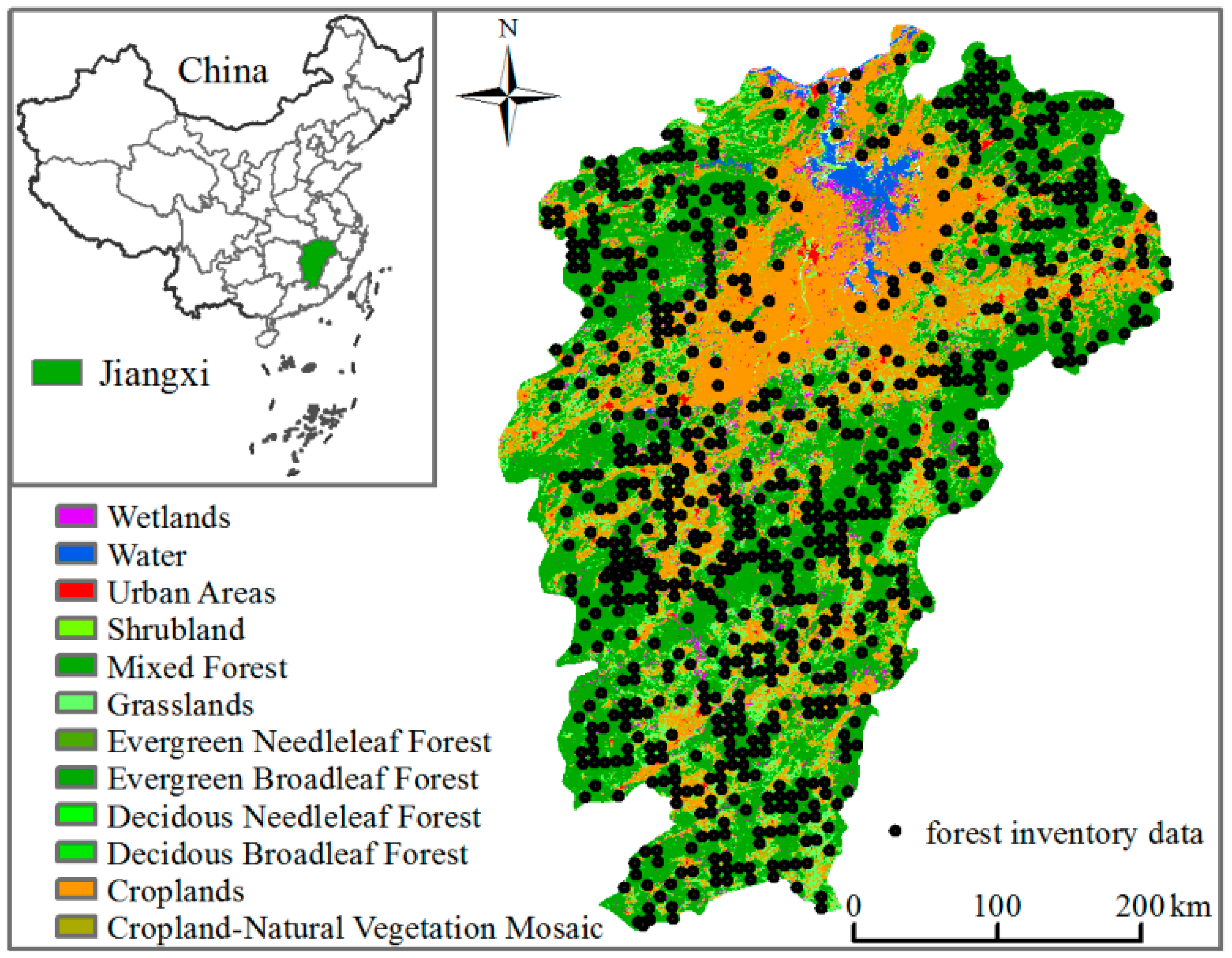
This study was conducted in Jiangxi Province, Southeast China (Figure 1). The MODIS land cover product (MOD12Q1) was applied as the vegetation classification data, as shown in Figure 1 [41]. This province is located at 24°29′ to 30°04′N and from 113°34′ to 118°28′E. Jiangxi Province has an area of 1.67 × 10⁵ km2 and a population of 45 million. It is located in a subtropical moisture monsoon climate zone and has an annual average temperature of ~16.3–17.5 °C and annual total precipitation of ~1341–1943 mm. The topography of Jiangxi is characterized by mountainous regions in the east, south, and west; plain and drainage in the north; and hilly and basin areas in the central part. Jiangxi Province currently has the second largest total forested area in China. According to the latest forest survey data, Jiangxi Province has a forest area of 1.021 × 10⁵ km2, with rich vegetation and typical subtropical evergreen broadleaf forests. Needle leaf forests, mixed needle and broadleaf forests, evergreen broadleaf forests, broadleaf mixed evergreen and deciduous forests, bamboo forests, and shrublands dominate the forested land.
2.2. Field Measurements
Forest reference data are critical for biomass estimation. In this study, the reference data were obtained from the Jiangxi Province section of National Forest Resource Inventory database for China [42]. The dataset was collected around 2006 (Figure 1). The plots were uniformly distributed over the forested land. Portable global positioning system (GPS) instruments and static differential GPS are widely used in field investigation [42]. The positioning error of the GPS was less than 7 m. Tree species were identified and the diameter at breast height (dbh) was measured for every tree with a dbh > 5 cm. Tree height was measured for 3–5 average trees in each plot. Heights were estimated by height–diameter models for trees that had not been measured in height. The biomass of each tree in the plots was estimated via allometry models for each tree species [43]. The biomass of each plot was the sum of the biomass predictions of all trees in the plot.
2.3. LiDAR Data
The GLAS staged in the ICESat emits a 1064 nm laser pulse at an elliptical ground footprint of ~64 m in diameter, and the echo waveform of the laser pulse is recorded by the sensor system [44]. The ellipsoidal footprints of ~65 m in diameter were spaced every 170 m along the track and at tens of kilometers across tracks [45]. In this study, we selected GLAS data from the operating periods L2B and L3A (from February 2006 to November 2006) for our forest AGB mapping procedure. Two GLAS products, GLA01 and GLA14, were downloaded from the ICESat/GLAS data pool and we recorded the full-waveform, surface elevation, location, and data quality for each laser shot. Four criteria were applied to the GLAS footprints to ensure their quality: (1) cloud free, (2) no saturation effects, (3) greater signal to noise ratios (SNRs), and (4) not significantly higher than the land surface elevation [46].
Pre-processing included error elimination, data decompression, voltage conversion, and filtering. The waveform was filtered using wavelet transform, which removes high-frequency noise and smooths the data. The leading edge extent, trailing edge extent, and waveform extent were computed from the full-waveform information of each laser shot. These three variables have been shown to be correlated with canopy height variability, terrain slope, and canopy height, respectively [47]. The methods used here to extract the GLAS waveform characteristics and correct the terrain followed those used by Xi et al. [22]. The wavelet analysis method was used to position the peak of the waveform and to extract waveform length information of the vegetation height peak.
2.4. MODIS Normalized Difference Vegetation Index Product (MOD13Q1)
Both the MODIS and Landsat TM data were downloaded and analyzed. Cloud-free, good-quality TM images that covered the study area in 2006 were lacking. The correlation coefficients between biomass and TM-Normalized Difference Vegetation Index (NDVI) were much less than MODIS-NDVI during March and September 2006. Therefore, we selected MODIS-Terra MOD13Q1 data as the source of the NDVI data. MOD13Q1 data are provided every 16 days at a 250-m spatial resolution. Jiangxi Province is covered by 3 MODIS path/row tiles (h28v05, h28v06, and h27v06). The data were corrected for the geometric and radiometric distortions of the images to the standard Level 1G before delivery. In this study, to explore the effectiveness of seasonal time series data for estimating forest AGB, the data from 15 MODIS images were acquired in different seasons (spanning from 81st to the 305th day of the year) for each path/row tile.
2.5. MODIS Percent Tree Cover Product (MOD44B)
The vegetation continuous fields collection (MOD44B) was used as the source of tree cover percentage data, which contains proportional estimates for woody vegetation cover types. Tree cover is predicted based on multi-temporal metrics for a full year using a regression tree model [48]. The RMSE is reported to be 9.06% for this collection. These data were included as an explanatory variable for the correlation between forest AGB and coverage.
3. Methods
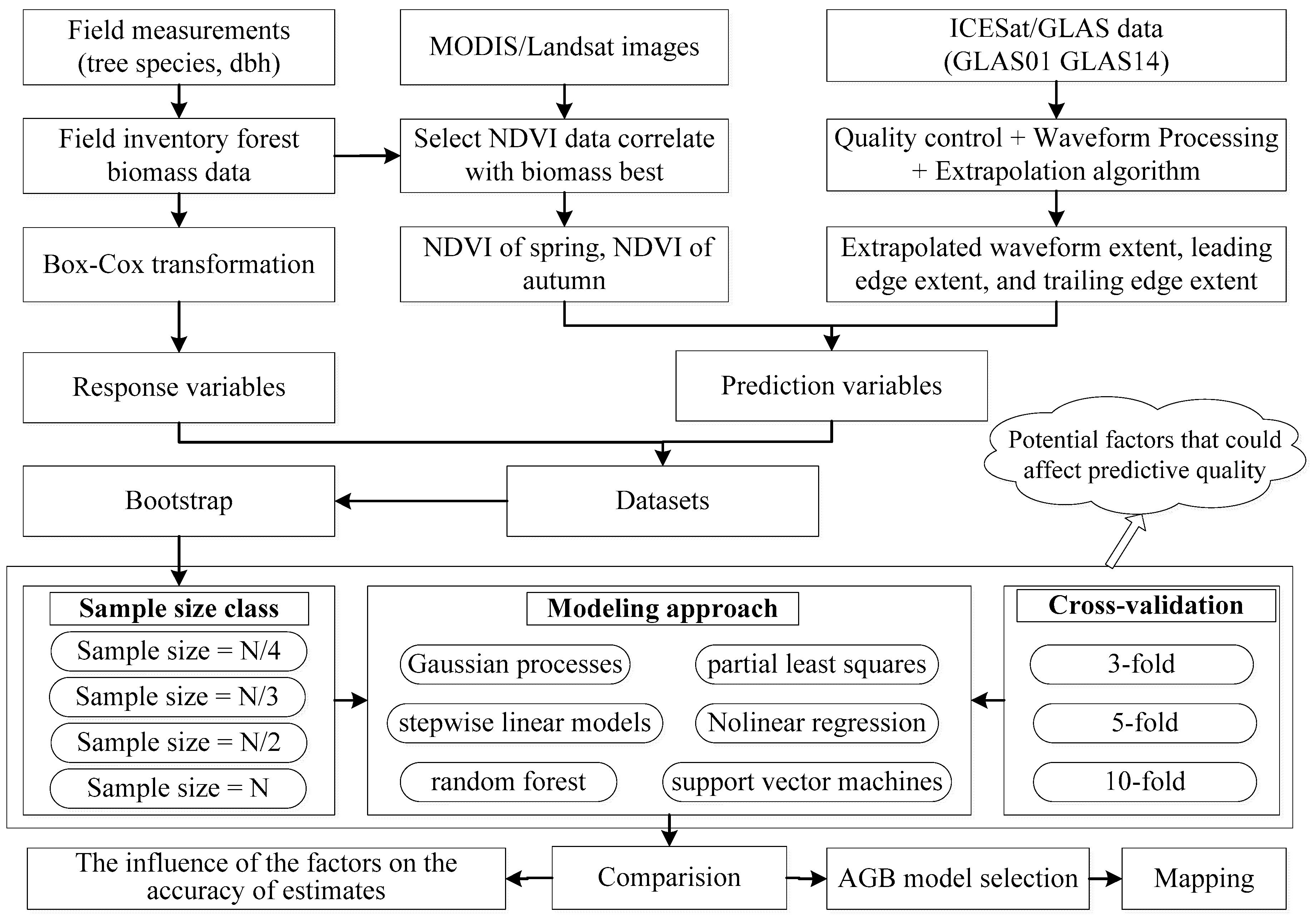
The methodology used to estimate forest AGB in this study is shown in Figure 2. The major steps include (1) extrapolating GLAS metrics and selecting MODIS variables (Section 3.1), (2) the creation of subsamples using bootstrapping technique (Section 3.2), (3) estimating forest AGB using different algorithms (Section 3.3), (4) comparing and evaluating the forest AGB estimating results, and (5) mapping the forest AGB over Jiangxi Province using the selected AGB algorithm.
3.1. Variables from GLAS and MODIS Data for Biomass Estimation
Since the spatial distance between two GLAS footprints was large, the probability of the collected reference data overlapping GLAS footprints was very small. To relate the GLAS variables to the reference data, three variables (leading edge extent, trailing edge extent, and waveform extent) were estimated into spatial continuous data using the random forest (RF) algorithm. Auxiliary predictors such as cumulative NDVI, elevation, slope, climate factors, and vegetation map were used in the RF modeling process. Detailed procedures used to estimate the three GLAS-derived variables can be found in Su et al. [8] and Lefsky [47], so they will not be discussed here.
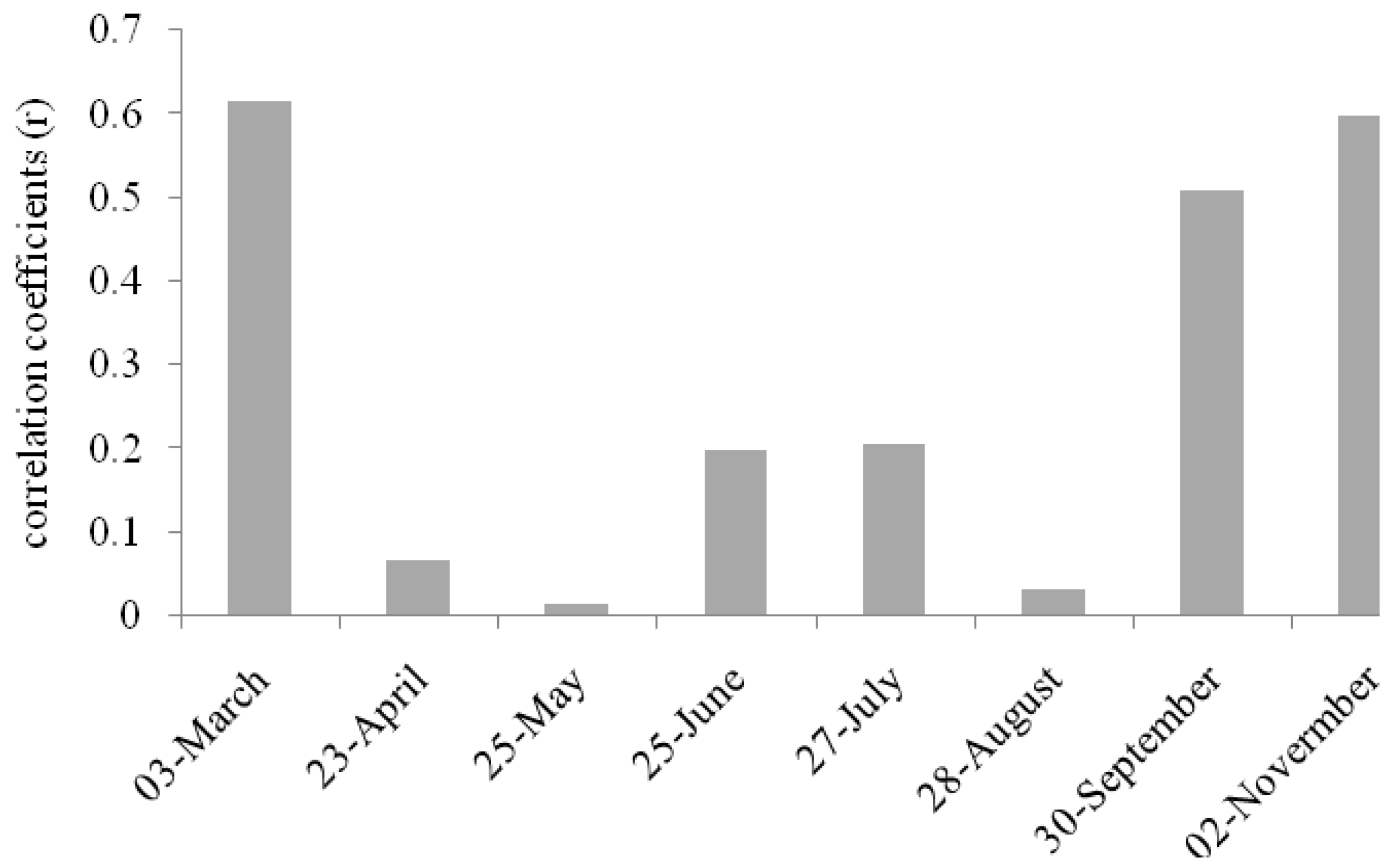
For the NDVI data, most existing studies chose the NDVI in peak season to estimate forest AGB; however, NDVI data collected at different times may provide different information regarding forest structure. Therefore, the capabilities of NDVI before or after peak season for forest AGB estimation should also be investigated. In this paper, correlation analysis was used to examine the relationships between ground-measured forest AGB and NDVI at different times. Figure 3 shows the correlation coefficients (r) between the forest field inventory biomass data and NDVI values at different times. The NDVI values in spring and autumn were more closely related to AGB than in the peak season in May, June, July, and August. In the peak season, the saturation issue for canopies with large density reduced the correlation between NDVI and AGB. Although vegetation indices in the months of the peak growth season have often been used in previous studies, they may not be the reasonable choice for biomass mapping. Data in March before the green up date and in November after the leaf senescence date are more closely related to AGB, because they contain information on tree stems and branches, and their density is related to AGB. In this study, the r value between NDVI in spring and autumn and AGB were larger (Figure 3). Therefore, NDVI in spring and autumn were selected as potential variables in the forest AGB prediction model.
Finally, six predictors were selected based on earlier experience and the literature review, including three GLAS variables, two NDVI, and the tree cover percent data. The value of these six predictors at the site of the reference data was estimated, and a 801 × 7 matrix of responses and predictor variables was prepared. The first column is reference data, and columns from the second to the seventh are the six predictors. There were 801 reference data points, corresponding to 801 rows.
3.2. Creation of Subsamples
Step 1: The matrix of the response and predictor variables was first ordered according to the biomass values in the first column. Then, the matrix was subdivided into five equal size subgroups. The size of the five subgroups was n/5, where n = 801.
Step 2: Bootstrapping was used to create subsamples from the stratified dataset in step 1 [49]. Four sample size classes were generated to test the influence of sample size on the performance of the prediction models. For each of the four desired sample size classes (nclass1 = n/4, nclass2 = n/3, nclass3 = n/2, nclass4 = n), 500 datasets were generated using replacement. The stratification procedure in step 1 ensured that samples from the full range of biomass values were included in each bootstrapped dataset.
3.3. Biomass Modeling Methods
For each sample size class, the 500 input datasets were fitted by six prediction algorithms: Gaussian processes (GPs), stepwise linear models (LMSTEP), partial least squares regression (PLS), nonlinear regression using a logistic model (NRL), random forest (RF), and support vector machine (SVM).
GPs provide a probabilistic approach for learning generic regression problems with kernels [50] and use a weighting strategy for the optimization, which is relevant to the predictor variables. The inverse of the specific variable controlling the spread of the relations for each particular predictor represents the relevance of that predictor variable. That is, the larger the variable, the more extended the relationships along that predictor (i.e., containing less informative content).
LMSTEP regression removes the least correlated variables using an iterative strategy, and finally obtains a regression model with the variables that most accurately explain the forest AGB [51]. In each step, a variable is considered for addition to or subtraction from the set of explanatory variables based on some pre-specified criterion, such as adjusted R2 and the Akaike information criterion.
PLS is based on linear transitions from several original variables to relatively few orthogonal factors or latent variables. It is useful for establishing predictive models when the predictor variables are collinear [52]. As metrics extracted from GLAS may be collinear, a PLS model was developed.
NRL should not be confused with the binomial logistic regression that is often used with categorical dataset. The mathematical form of the NRL model is given by [53].
SVM is a typical nonparametric algorithm [54] that transforms a nonlinear regression into a linear regression using a kernel function. In this paper, the radial basis function kernel was selected for forest AGB prediction, since it requires fewer parameters and can reduce the complexity of numerical calculation.
RF regression has been successfully used in ecological remote sensing areas such as biomass estimation. RF constructs numerous independent regression trees, and a bootstrapping sample is chosen for each regression tree. The regression tree continues to grow until it reaches the largest size. The results are estimated by averaging the predictions of all regression trees [55].
For each of the prediction algorithms, as well as each sample size class, k-fold cross-validation was performed, which produced the diagnostics RMSE and coefficient of determination (R2). In this study, cross-validation was applied with three settings (3-fold, 5-fold, and 10-fold) to test the influence of different settings on the results. The relative error index was calculated using the following equation to measure the accuracy of prediction:
where is the predicted AGB, is the observed value, and n is the number of validation samples.
Analysis of variance (ANOVA) was used to estimate the contribution of each of the three factors (prediction method, sample size, and number of folds) and their interactions to the model diagnostics (R2 and RMSE) [56].
4. Results
4.1. ANOVA Results
The maximum sum of squares values are the reported for the prediction method (76.34) and sample size (12.65) as well as for their interaction (18.52) (Table 1). The sum of squares value indicates the contribution of the factor in describing the variance of R2 and RMSE; a larger value indicates a more important contribution. The number of folds in the k-fold cross-validation settings was less important than the prediction method and sample size, as indicated by the smaller sum of squares (3.58). ANOVA results for RMSE showed the same pattern, with the prediction model and sample size as well as their interaction having the larger sum of squares values (5013184, 22048, and 53584, respectively). The number of folds did not notably contribute to the model diagnostics (the sum of squares value was 148 for RMSE).
4.2. Model Performance
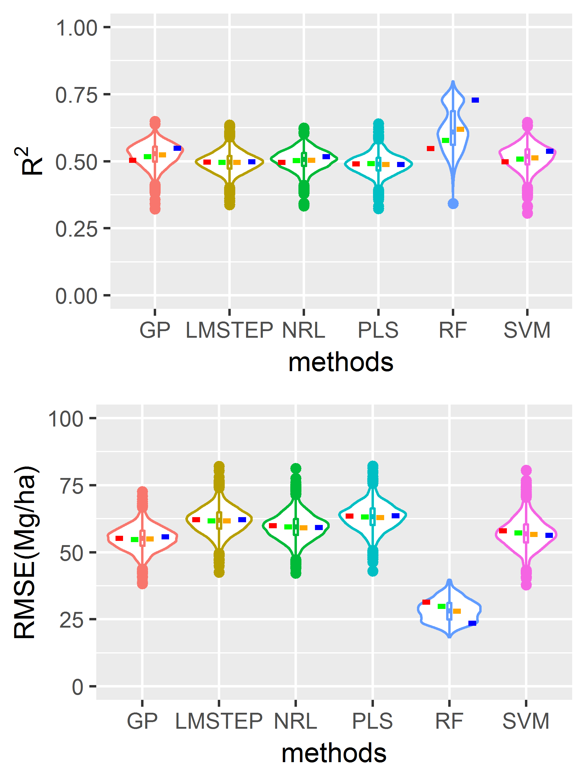
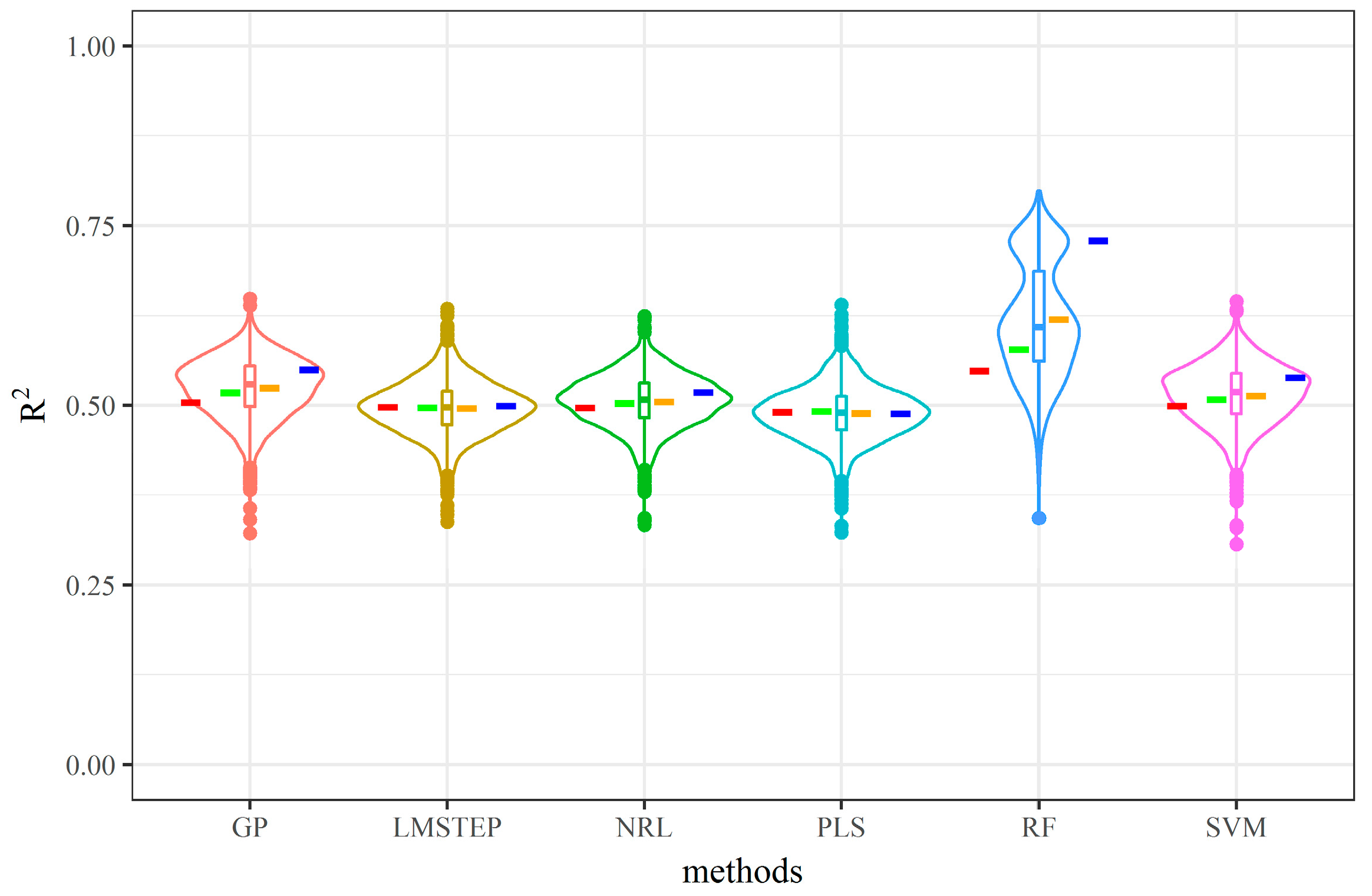
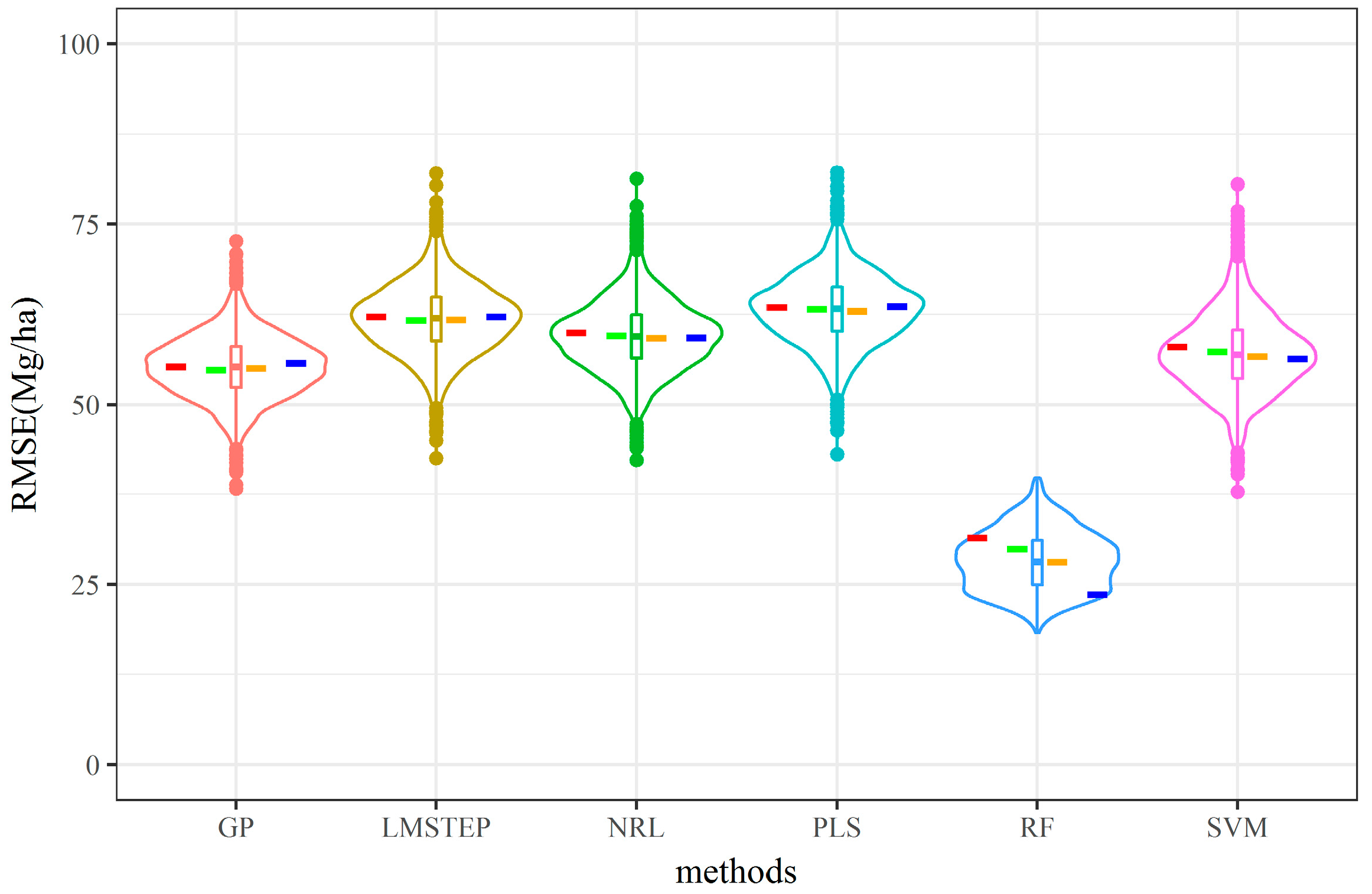
Figure 4 and Figure 5 summarize the model performance obtained from all model runs. The violin plots in Figure 4 illustrate the distribution of the R2 values obtained by five-fold cross-validation for the six methods. Each of the methods had four sample size classes. The R2 values for each of the four sample size classes were obtained from 500 bootstrapped models. The median R2 values for each of the four sample size classes are presented with colored horizontal stripes. Class 1 to 4 from left to right are shown in red, green, orange, and blue respectively. The violin plots in Figure 5 illustrate the distribution of the RMSE values, and explanations follow those for Figure 4. A comparison of the six prediction methods indicated that RF provided more accurate AGB estimates than the other five methods, especially when a larger sample size was available. Concerning the sample size, a stable increase in accuracy and decrease in RMSE were observed along with an increasing number of sample units (colored horizontal stripes from left to right). Exceptions were the RMSE values of the GP and PLS methods, where a slight increase in RMSE was observed when switching from class 3 to class 4 with the largest number of sample units. The absolute differences in R2 and RMSE between RF and the second model ranged from 0.04 and 23.78 Mg/ha (class 1, second model GP) to 0.18 and 32.16 Mg/ha (class 4, second model GP). The absolute differences in R2 and RMSE between RF and the least accurate prediction model (PLS) were 0.24 and 40.02 Mg/ha, respectively. GP and SVM produced larger R2 and smaller RMSE when compared to NRL, PLS, and LMSTEP in most cases.
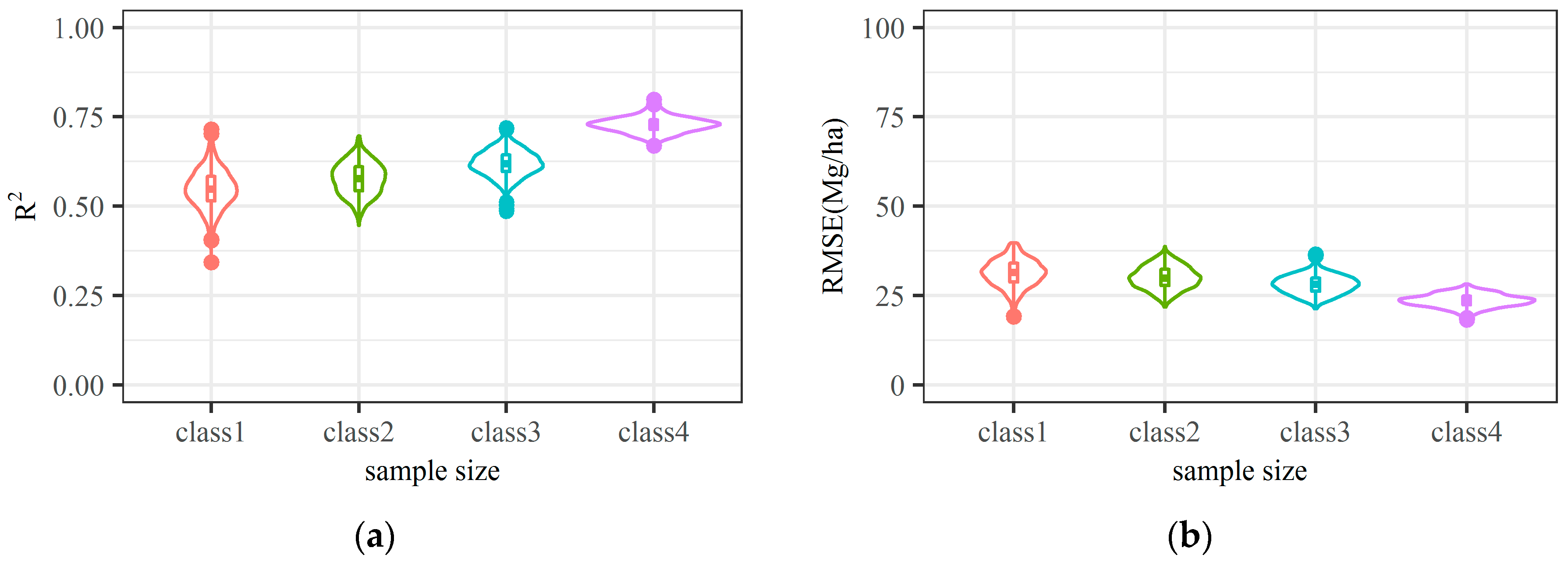
A downside was that RF showed the largest variances in the obtained R2 values when four classes of sample size were all used (Figure 4). However, the ranges of the variation in R2 and RMSE reduced when the sample sizes increased (Figure 6).
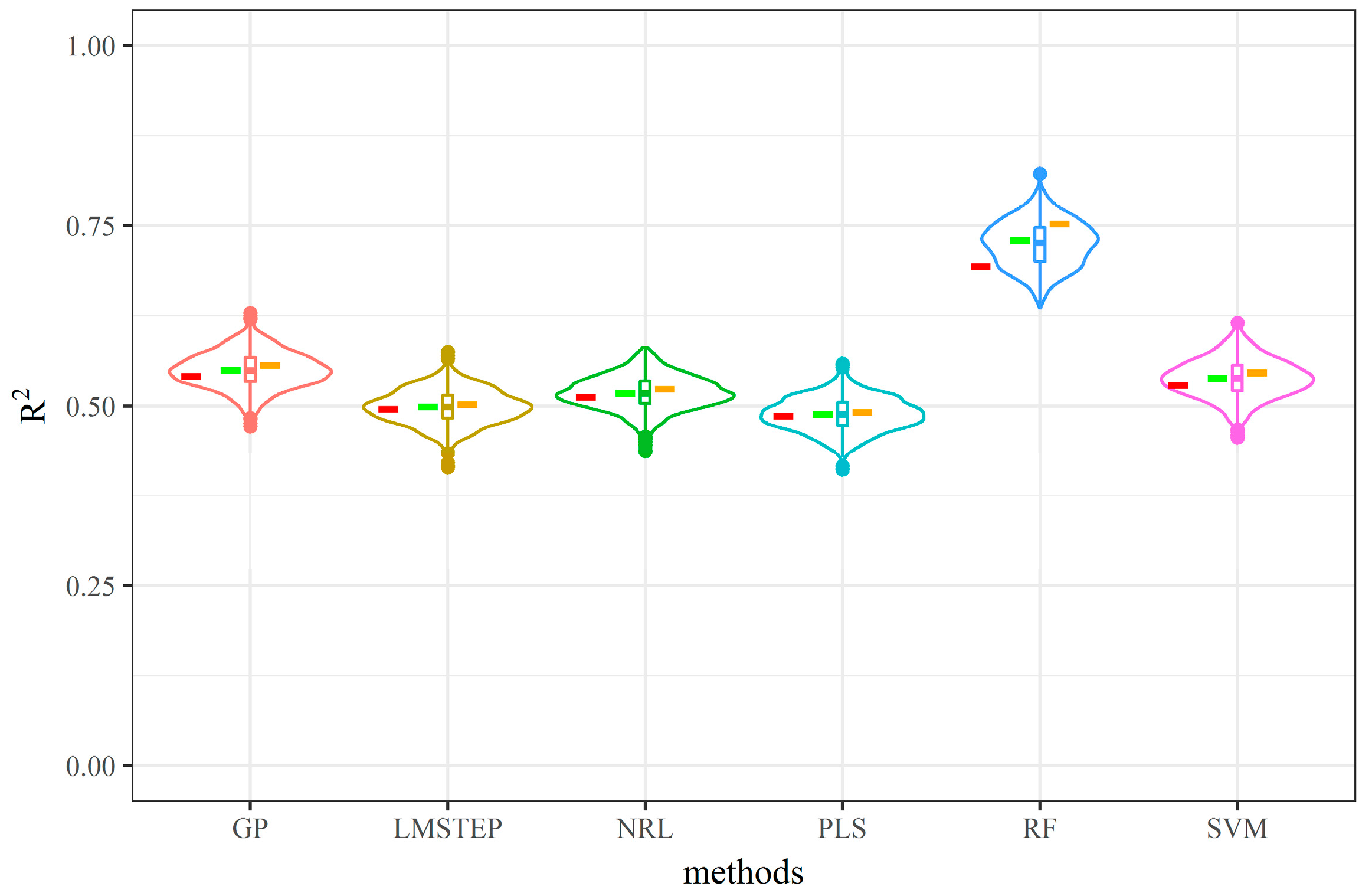
The modeling accuracy results of the six prediction methods created with different cross-validation settings are presented in Figure 7 and Figure 8. The violin plots in Figure 7 and Figure 8 illustrate the distribution of R2 and RMSE values, respectively, from the 500 bootstrapped models as obtained by 3-fold, 5-fold, and 10-fold cross-validation for each method using the class 4 dataset. The median values of R2 or RMSE for 3-fold, 5-fold, and 10-fold cross-validation are presented from left to right in red, green and orange horizontal stripes. In most cases, a larger number of folds led to an obvious increase in R2. However, the difference in RMSE resulting from the different number of folds was very small (Figure 8).
To validate the prediction accuracy of the different methods, the mean relative error indices were calculated (Table 2). The sample sizes in class 1 to class 4 were n/4, n/3, n/2, and n respectively. A prediction technique with a smaller relative error is more accurate. The results showed that RF was more accurate than the other methods, followed by GPs, NRL, SVM, LMSTEP, and PLS in sequence. The relative error decreased when the sample sizes increased in the RF method, but this trend was not obvious for the other methods.
4.3. Mapping Forest Aboveground Biomass
The spatial distribution of forest AGB over the study area is shown in Figure 9, which was obtained using the RF model with the largest number of sample units. The forest AGB density was distributed mainly within the 60–180 Mg/ha. Figure 9 shows clear spatial patterns in the study area of the AGB values. Greater AGB values were distributed in South and Northeast Jiangxi, which are mountainous areas. The total AGB of all forest types estimated with RF was 9.19 × 10⁸ Mg in Jiangxi Province. A comparison between the different forest types showed that the evergreen broadleaf forest had the largest mean AGB value (112.57 Mg/ha). Evergreen needle-leaf and deciduous needle-leaf forests had smaller mean AGB values (32.40 and 25.63 Mg/ha, respectively), and the least AGB estimates were found in shrubland (15.25 Mg/ha).
5. Discussion
Although many studies of forest AGB estimation have been conducted, substantial uncertainties remain in the current estimations. In this study, we analyzed the effects of the prediction method (six cases), sample size (four cases), and cross-validation (three cases) on the prediction quality of forest AGB estimation from LiDAR and optical remote sensing data. We generated subsamples using stratified bootstrapping. The ANOVA method was used to rank the importance of the three factors on the accuracy of the biomass predictions reflected in the computed diagnostics (RMSE and R2).
The ANOVA results showed that the prediction method was the most important factor affecting the quality of the biomass estimation. This is in line with earlier studies [33,57,58] that reported notable differences in the performance of the prediction methods.
The performance of the six prediction methods was compared in this study, including three parameter methods (LMSTEP, PLS, and NRL) and three nonparametric methods (GPs, RF, and SVM). Among the parameter methods, LMSTEP and PLS are classified as linear regression and NRL is classified as nonlinear regression. RF provided the greatest estimation accuracy in terms of the largest R2, the smallest RMSE, and the smallest relative error, especially when a larger sample size was used. This result complements those of other studies [10,40,57,58]. One of the main advantages of RF is its flexibility due to its conceptual design, which differs from all the other five models. A downside of RF may be that when a small size sample is applied in the algorithm, the variance of estimates is considerable. An increase in sample size can lead to a reduction in the range of variation. Among the three nonparametric algorithms in this study, GPs generated suboptimal predicted results in terms of R2, RMSE, and relative error. The SVM showed the least favorable accuracy, which is consistent with the conclusions from recent studies [59,60].
The linear regression methods LMSTEP and PLS, provided less accurate estimates than the nonparametric algorithms RF, GPs, and SVM, in most cases, which was in line with the findings of other studies [34]. In addition, no improvement occurred when larger size samples were used for these two methods. This can be explained by the fact that the relationship between remote sensing predictors and observed forest biomass is likely to be nonlinear and therefore not well modeled. Linear regression based on remote sensing data may be more suitable for predicting vegetation AGB in other biomes such as grasslands. The NRL was more accurate than LMSTEP and PLS in terms of relative error.
The sample size was less important than the prediction method for explaining the variance of model diagnostics RMSE and R2. The R2 values increased along with the increasing number of sample units for the nonparametric algorithms, especially for RF. The RMSE decreased with increasing number of sample units, except for GPs from class 3 to class 4. Therefore, model estimates can be improved by increasing the sample size rather than improving the prediction algorithms. Since field data are costly to obtain and limited, other choices such as realistic synthetic datasets present an interesting alternative to field data [61]. Huang et al. [23] constructed allometric models using limited field plots and transmitted the ecological information to GLAS data. They enriched the AGB samples into the number of GLAS spots. They also stated that more training samples may be helpful in developing a robust RF model for mapping forest AGB, despite the uncertainties introduced by AGB in GLAS spots.
The number of folds was found to have an effect on the explained variance in R2. Increasing the number of folds within the cross-validation settings improved the R2 values, especially for the three nonparametric algorithms (RF, GPs, and SVM). For model runs with a large number of folds (for example, 10 folds) may produce larger R2 values, which overestimate the predictive power of the models. We concluded that the small sample size of the hold out sample during the cross-validation using a large number of folds caused this result. Most previous studies ignored the influence of the number of folds. When the results from different studies are compared, the number of folds in the cross-validation settings should be considered. RMSE values were more robust than R2 values to the validation settings, and no apparent change occurred in RMSE under different numbers of folds.
The results should be interpreted cautiously as the study was limited to one site. This conclusion may change if other sites with different forest structure, tree species, and topography are tested. In addition, ANOVA assumes that the dependent variable is subjected to non-negligible error. The response variables in this study were sample-based estimates subjected to sampling variability. ANOVA was used as a diagnostic tool in this study, but the significance level was small. Furthermore, the allometric models led to uncertainties in biomass estimates. We tried to improve the accuracy via using allometric models for each tree species of the study area. However, there were still some uncertainties because tree densities, soil texture, and climate conditions may influence the growth of tree height and dbh, thus influencing the accumulation of biomass.
Further studies could investigate whether other datasets, such as radar, could alter our finding. An additional research issue to be tackled is the comparison of methods relative to the width of the confidence intervals rather than to the quality of fit of the models to the data. Considering the limitations of the available reference samples, improving the statistical algorithms or developing a new prediction method would be helpful for minimizing the predictive error of forest AGB. We are now developing a new prediction algorithm, called high accuracy surface modeling, which has the potential to improve the prediction accuracy.
6. Conclusions
We illustrated the forest AGB estimation through a comparative analysis of different prediction methods (GPs, NRL, LMSTEP, PLS, RF, and SVM) based on field measurements, LiDAR and optical data. The effects of the prediction method, sample size, and cross-validation setting were compared and analyzed using two remote sensing datasets combined with stratified bootstrapping. We found that the prediction method had a considerable effect on the accuracy of the biomass estimates, being more important than sample size. The number of folds in the cross-validation setting was a less important factor than prediction method and sample size. The model diagnostic R2 was influenced notably by the number of folds. The estimate produced with the RF algorithm was more accurate than the other five AGB models in this study. In most cases, the increase in the sample size led to an increase in the accuracy of the estimation. The RF algorithm notably benefits from a larger sample size. Finally, the forest AGB was mapped using the RF model with all the reference data. Choosing an appropriate prediction method is recommended to improve the predictive accuracy. The influence of the number of folds should be considered when comparing model performance.
Author Contributions
Conceptualization, M.W.; Data curation, G.L.; Formal analysis, X.S.; Funding acquisition, X.S.; Methodology, X.S.; Resources, G.L.; Supervision, M.W.; Validation, M.W.; Writing—original draft, X.S.; Writing—review and editing, M.W. and Z.F.
Funding
This research was funded by the National Key Research and Development Program of China (Grant No. 2016YFA0600204), National Natural Science Foundation of China (Grant No. 41501428, 41371400), Natural Science Foundation of Shandong Province, China (Grant No. ZR2017BD010), and the Project of Shandong Province Higher Educational Science and Technology Program (Grant No. J16LH01).
Acknowledgments
The authors would like to express gratitude to Tianyu Hu and Yanjun Su from Institute of Botany, the Chinese Academy of Sciences, who provide much help and instruction in GLAS data processing.
Conflicts of Interest
The authors declare no conflict of interest.
References
- Le Toan, T.; Quegan, S.; Davidson, M.; Balzter, H.; Paillou, P.; Papathanassiou, K.; Plummer, S.; Rocca, F.; Saatchi, S.; Shugart, H. The BIOMASS mission: Mapping global forest biomass to better understand the terrestrial carbon cycle. Remote Sens. Environ. 2011, 115, 2850–2860. [Google Scholar] [CrossRef] [Green Version]
- Pettorelli, N.; Wegmann, M.; Skidmore, A.; Mücher, S.; Dawson, T.P.; Fernandez, M.; Lucas, R.; Schaepman, M.E.; Wang, T.; O’Connor, B. Framing the concept of satellite remote sensing essential biodiversity variables: Challenges and future directions. Remote Sens. Ecol. Conserv. 2016, 2, 122–131. [Google Scholar] [CrossRef]
- Lu, D.; Chen, Q.; Wang, G.; Liu, L.; Li, G.; Moran, E. A survey of remote sensing-based aboveground biomass estimation methods in forest ecosystems. Int. J. Digit. Earth 2014, 9, 63–105. [Google Scholar] [CrossRef]
- Sullivan, M.J.P.; Lewis, S.L.; Hubau, W.; Lan, Q.; Phillips, O.L. Field methods for sampling tree height for tropical forest biomass estimation. Methods Ecol. Evol. 2018, 9, 1179–1189. [Google Scholar] [CrossRef] [Green Version]
- Zhao, P.; Lu, D.; Wang, G.; Liu, L.; Li, D.; Zhu, J.; Yu, S. Forest aboveground biomass estimation in zhejiang province using the integration of landsat tm and alos palsar data. Int. J. Appl. Earth Obs. Geoinf. 2016, 53, 1–15. [Google Scholar] [CrossRef]
- Maire, G.L.; Marsden, C.; Nouvellon, Y.; Grinand, C.; Hakamada, R.; Stape, J.L.; Laclau, J.P. Modis ndvi time-series allow the monitoring of eucalyptus plantation biomass. Remote Sens. Environ. 2011, 115, 2613–2625. [Google Scholar] [CrossRef]
- Chi, H.; Sun, G.; Huang, J.; Guo, Z.; Ni, W.; Fu, A. National forest aboveground biomass mapping from icesat/glas data and modis imagery in china. Remote Sens. 2015, 7, 5534–5564. [Google Scholar] [CrossRef]
- Su, Y.; Guo, Q.; Xue, B.; Hu, T.; Alvarez, O.; Tao, S.; Fang, J. Spatial distribution of forest aboveground biomass in china: Estimation through combination of spaceborne lidar, optical imagery, and forest inventory data. Remote Sens. Environ. 2016, 173, 187–199. [Google Scholar] [CrossRef]
- Tian, X.; Yan, M.; Tol, C.V.D.; Li, Z.; Su, Z.; Chen, E.; Li, X.; Li, L.; Wang, X.; Pan, X. Modeling forest above-ground biomass dynamics using multi-source data and incorporated models: A case study over the qilian mountains. Agric. For. Meteorol. 2017, 246, 1–14. [Google Scholar] [CrossRef]
- Liu, K.; Wang, J.; Zeng, W.; Song, J. Comparison and evaluation of three methods for estimating forest above ground biomass using tm and glas data. Remote Sens. 2017, 9, 341. [Google Scholar] [CrossRef]
- Gao, Y.; Lu, D.; Li, G.; Wang, G.; Chen, Q.; Liu, L.; Li, D. Comparative analysis of modeling algorithms for forest aboveground biomass estimation in a subtropical region. Remote Sens. 2018, 10, 627. [Google Scholar] [CrossRef]
- Bourgoin, C.; Blanc, L.; Bailly, J.-S.; Cornu, G.; Berenguer, E.; Oszwald, J.; Tritsch, I.; Laurent, F.; Hasan, A.; Sist, P.; et al. The potential of multisource remote sensing for mapping the biomass of a degraded amazonian forest. Forests 2018, 9, 303. [Google Scholar] [CrossRef]
- Zhu, X.; Liu, D. Improving forest aboveground biomass estimation using seasonal landsat ndvi time-series. ISPRS J. Photogramm. Remote Sens. 2015, 102, 222–231. [Google Scholar] [CrossRef]
- Feng, Y.; Lu, D.; Chen, Q.; Keller, M.; Moran, E.; Dossantos, M.N.; Bolfe, E.L.; Batistella, M. Examining effective use of data sources and modeling algorithms for improving biomass estimation in a moist tropical forest of the brazilian amazon. Int. J. Digit. Earth 2017, 10, 996–1016. [Google Scholar] [CrossRef]
- Mahmudurrahman, M.; Sumantyo, J.T.S. Retrieval of tropical forest biomass information from alos palsar data. Geocarto Int. 2013, 28, 382–403. [Google Scholar]
- Shen, W.; Li, M.; Huang, C.; Tao, X.; Wei, A. Annual forest aboveground biomass changes mapped using icesat/glas measurements, historical inventory data, and time-series optical and radar imagery for guangdong province, china. Agric. For. Meteorol. 2018, 259, 23–38. [Google Scholar] [CrossRef]
- Myneni, R.B.; Dong, J.; Tucker, C.J.; Kaufmann, R.K.; Kauppi, P.E.; Liski, J.; Zhou, L.; Alexeyev, V.; Hughes, M.K. A large carbon sink in the woody biomass of northern forests. Proc. Natl. Acad. Sci. USA 2001, 98, 14784–14789. [Google Scholar] [CrossRef] [PubMed]
- Lu, D. The potential and challenge of remote sensing-based biomass estimation. Int. J. Remote Sens. 2006, 27, 1297–1328. [Google Scholar] [CrossRef]
- Woodhouse, I.H.; Mitchard, E.T.A.; Brolly, M.; Maniatis, D.; Ryan, C.M. Radar backscatter is not a ‘direct measure’ of forest biomass. Nat. Clim. Chang. 2012, 2, 556–557. [Google Scholar] [CrossRef]
- Véga, C.; Vepakomma, U.; Morel, J.; Bader, J.-L.; Rajashekar, G.; Jha, C.S.; Ferêt, J.; Proisy, C.; Pélissier, R.; Dadhwal, V.K. Aboveground-biomass estimation of a complex tropical forest in india using lidar. Remote Sens. 2015, 7, 10607–10625. [Google Scholar] [CrossRef]
- Zhao, K.; Suarez, J.C.; Garcia, M.; Hu, T.; Wang, C.; Londo, A. Utility of multitemporal lidar for forest and carbon monitoring: Tree growth, biomass dynamics, and carbon flux. Remote Sens. Environ. 2018, 204, 883–897. [Google Scholar] [CrossRef]
- Xi, X.; Han, T.; Cheng, W.; Luo, S.; Pan, F. Forest above ground biomass inversion by fusing glas with optical remote sensing data. Isprs Int. J. Geo-Inf. 2016, 5, 45. [Google Scholar] [CrossRef]
- Huang, H.; Liu, C.; Wang, X.; Zhou, X.; Gong, P. Integration of multi-resource remotely sensed data and allometric models for forest aboveground biomass estimation in China. Remote Sens. Environ. 2019, 221, 225–234. [Google Scholar] [CrossRef]
- Nelson, R. Model effects on glas-based regional estimates of forest biomass and carbon. Int. J. Remote Sens. 2010, 31, 1359–1372. [Google Scholar] [CrossRef]
- Zolkos, S.; Goetz, S.; Dubayah, R. A meta-analysis of terrestrial aboveground biomass estimation using lidar remote sensing. Remote Sens. Environ. 2013, 128, 289–298. [Google Scholar] [CrossRef]
- Zhao, M.; Yue, T.; Na, Z.; Sun, X.; Zhang, X. Combining lpj-guess and hasm to simulate the spatial distribution of forest vegetation carbon stock in china. J. Geogr. Sci. 2014, 24, 249–268. [Google Scholar] [CrossRef]
- Dormann, C.F.; Schymanski, S.J.; Cabral, J.; Chuine, I.; Graham, C.; Hartig, F.; Kearney, M.; Morin, X.; Römermann, C.; Schröder, B. Correlation and process in species distribution models: Bridging a dichotomy. J. Biogeogr. 2012, 39, 2119–2131. [Google Scholar] [CrossRef]
- Gasparri, N.I.; Parmuchi, M.G.; Bono, J.; Karszenbaum, H.; Montenegro, C.L. Assessing multi-temporal landsat 7 etm+ images for estimating above-ground biomass in subtropical dry forests of argentina. J. Arid Environ. 2010, 74, 1262–1270. [Google Scholar] [CrossRef]
- Hansen, M.C.; Potapov, P.V.; Moore, R.; Hancher, M.; Turubanova, S.; Tyukavina, A.; Thau, D.; Stehman, S.; Goetz, S.; Loveland, T. High-resolution global maps of 21st-century forest cover change. Science 2013, 342, 850–853. [Google Scholar] [CrossRef] [PubMed]
- Powell, S.L.; Cohen, W.B.; Healey, S.P.; Kennedy, R.E.; Moisen, G.G.; Pierce, K.B.; Ohmann, J.L. Quantification of live aboveground forest biomass dynamics with landsat time-series and field inventory data: A comparison of empirical modeling approaches. Remote Sens. Environ. 2010, 114, 1053–1068. [Google Scholar] [CrossRef]
- Ingram, J.C.; Dawson, T.P.; Whittaker, R.J. Mapping tropical forest structure in southeastern madagascar using remote sensing and artificial neural networks. Remote Sens. Environ. 2005, 94, 491–507. [Google Scholar] [CrossRef]
- Cutler, M.E.J.; Boyd, D.S.; Foody, G.M.; Vetrivel, A. Estimating tropical forest biomass with a combination of sar image texture and landsat tm data: An assessment of predictions between regions. ISPRS J. Photogramm. Remote Sens. 2012, 70, 66–77. [Google Scholar] [CrossRef]
- Gleason, C.J.; Im, J. Forest biomass estimation from airborne lidar data using machine learning approaches. Remote Sens. Environ. 2012, 125, 80–91. [Google Scholar] [CrossRef]
- Zhang, Y.; Liang, S.; Sun, G. Forest biomass mapping of northeastern china using glas and modis data. IEEE J. Sel. Top. Appl. Earth Obs. Remote Sens. 2014, 7, 140–152. [Google Scholar] [CrossRef]
- Chen, Q.; McRoberts, R.E.; Wang, C.; Radtke, P.J. Forest aboveground biomass mapping and estimation across multiple spatial scales using model-based inference. Remote Sens. Environ. 2016, 184, 350–360. [Google Scholar] [CrossRef]
- Fayad, I.; Baghdadi, N.; Guitet, S.; Bailly, J.S.; Hérault, B.; Gond, V.; Hajj, M.E.; Minh, D.H.T. Aboveground biomass mapping in french guiana by combining remote sensing, forest inventories and environmental data. Int. J. Appl. Earth Obs. Geoinf. 2016, 52, 502–514. [Google Scholar] [CrossRef]
- McRoberts, R.E.; Næsset, E.; Gobakken, T. Optimizing the k-nearest neighbors technique for estimating forest aboveground biomass using airborne laser scanning data. Remote Sens. Environ. 2015, 163, 13–22. [Google Scholar] [CrossRef]
- Yue, T.X.; Wang, Y.F.; Du, Z.P.; Zhao, M.W.; Zhang, L.L.; Zhao, N.; Lu, M.; Larocque, G.R.; Wilson, J.P. Analysing the uncertainty of estimating forest carbon stocks in china. Biogeosciences 2016, 13, 3991–4004. [Google Scholar] [CrossRef]
- Stone, M. Cross-validatory choice and assessment of statistical predictions. J. R. Stat. Soc. 1974, 36, 111–147. [Google Scholar] [CrossRef]
- Fassnacht, F.E.; Hartig, F.; Latifi, H.; Berger, C.; Hernández, J.; Corvalán, P.; Koch, B. Importance of sample size, data type and prediction method for remote sensing-based estimations of aboveground forest biomass. Remote Sens. Environ. 2014, 154, 102–114. [Google Scholar] [CrossRef]
- Cracknell, A.P.; Kanniah, K.D.; Tan, K.P.; Lei, W. Towards the development of a regional version of MOD17 for the determination of gross and net primary productivity of oil palm trees. Int. J. Remote Sens. 2015, 36, 262–289. [Google Scholar] [CrossRef] [Green Version]
- Xie, X.; Wang, Q.; Dai, L.; Su, D.; Wang, X.; Qi, G.; Ye, Y. Application of China’s National Forest Continuous Inventory Database. Environ. Manag. 2011, 48, 1095–1106. [Google Scholar] [CrossRef] [PubMed]
- Wang, Y.F.; Yue, T.X.; Lei, Y.C.; Du, Z.P.; Zhao, M.W. Uncertainty of forest biomass carbon patterns simulation on provincial scale: A case study in jiangxi province, china. J. Geogr. Sci. 2016, 26, 568–584. [Google Scholar] [CrossRef]
- Abshire, J.B.; Sun, X.; Riris, H.; Sirota, J.M.; Mcgarry, J.F.; Palm, S.; Yi, D.; Liiva, P. Geoscience laser altimeter system (glas) on the icesat mission: On-orbit measurement performance. Geophys. Res. Lett. 2003, 32. [Google Scholar] [CrossRef]
- Schutz, B.E.; Zwally, H.J.; Shuman, C.A.; Hancock, D.; Dimarzio, J.P. Overview of the icesat mission. Geophys. Res. Lett. 2005, 32, 97–116. [Google Scholar] [CrossRef]
- Hu, T.; Su, Y.; Xue, B.L.; Liu, J.; Zhao, X.; Fang, J.; Guo, Q. Mapping global forest aboveground biomass with spaceborne lidar, optical imagery, and forest inventory data. Remote Sens. 2016, 8, 565. [Google Scholar] [CrossRef]
- Lefsky, M.A. A global forest canopy height map from the moderate resolution imaging spectroradiometer and the geoscience laser altimeter system. Geophys. Res. Lett. 2010, 37. [Google Scholar] [CrossRef]
- Wang, Y.; Li, G.; Ding, J.; Guo, Z.; Tang, S.; Wang, C.; Huang, Q.; Liu, R.; Chen, J.M. A combined glas and modis estimation of the global distribution of mean forest canopy height. Remote Sens. Environ. 2016, 174, 24–43. [Google Scholar] [CrossRef]
- Wehrens, R.; Putter, H.; Buydens, L.M.C. The bootstrap: A tutorial. Chemom. Intell. Lab. Syst. 2000, 54, 35–52. [Google Scholar] [CrossRef]
- Rasmussen, C.E.; Williams, C.K.I. Gaussian Processes for Machine Learning; The MIT Press: New York, NY, USA, 2006. [Google Scholar]
- Tian, X.; Su, Z.; Chen, E.; Li, Z.; van der Tol, C.; Guo, J.; He, Q. Estimation of forest above-ground biomass using multi-parameter remote sensing data over a cold and arid area. Int. J. Appl. Earth Obs. Geoinf. 2012, 17, 102–110. [Google Scholar] [CrossRef]
- Rocha de Souza Pereira, F.; Kampel, M.; Gomes Soares, M.L.; Estrada, G.C.D.; Bentz, C.; Vincent, G. Reducing uncertainty in mapping of mangrove aboveground biomass using airborne discrete return lidar data. Remote Sens. 2018, 10, 637. [Google Scholar] [CrossRef]
- Mcroberts, R.E.; Næsset, E.; Gobakken, T. Inference for lidar-assisted estimation of forest growing stock volume. Remote Sens. Environ. 2013, 128, 268–275. [Google Scholar] [CrossRef]
- Mountrakis, G.; Im, J.; Ogole, C. Support vector machines in remote sensing: A review. ISPRS J. Photogramm. Remote Sens. 2011, 66, 247–259. [Google Scholar] [CrossRef]
- Breiman, L. Random forests. Mach. Learn. 2001, 45, 5–32. [Google Scholar] [CrossRef]
- Tabachnick, B.G.; Fidell, L.S. Using Multivariate Statistics, 5th ed.; Pearson: Boston, MA, USA, 2007. [Google Scholar]
- García-Gutiérrez, J.; González-Ferreiro, E.; Mateos-García, D.; Riquelme-Santos, J.C.; Miranda, D. A Comparative Study between Two Regression Methods on Lidar Data: A Case Study; Springer: Berlin/Heidelberg, Germany, 2011; pp. 311–318. [Google Scholar]
- Latifi, H.; Nothdurft, A.; Koch, B. Non-parametric prediction and mapping of standing timber volume and biomass in a temperate forest: Application of multiple optical/lidar-derived predictors. Forestry 2010, 83, 1–5. [Google Scholar] [CrossRef]
- Cao, L.; Pan, J.; Li, R.; Li, J.; Li, Z. Integrating Airborne LiDAR and Optical Data to Estimate Forest Aboveground Biomass in Arid and Semi-Arid Regions of China. Remote Sens. 2018, 10, 532. [Google Scholar] [CrossRef]
- Wang, M.; Sun, R.; Xiao, Z. Estimation of Forest Canopy Height and Aboveground Biomass from Spaceborne LiDAR and Landsat Imageries in Maryland. Remote Sens. 2018, 10, 344. [Google Scholar] [CrossRef]
- Fassnacht, F.E.; Latifi, H.; Hartig, F. Using synthetic data to evaluate the benefits of large field plots for forest biomass estimation with lidar. Remote Sens. Environ. 2018, 213, 115–128. [Google Scholar] [CrossRef]
Figure 1.
The location (upper left) of Jiangxi Province and its vegetation distribution.

Figure 2.
Schematic representation of the main methods followed in this study. Moderate Resolution Imaging Spectroradiometer (MODIS); Normalized Difference Vegetation Index (NDVI); diameter at breast height (dbh); Ice, Cloud, and land Elevation Satellite (ICESat), Geoscience Laser Altimeter System (GLAS), aboveground biomass (AGB).

Figure 3.
Correlation coefficients (r) between biomass and NDVI on different dates.

Figure 4.
The distribution of R2 values using different prediction approaches.

Figure 5.
The distribution of RMSE values using different prediction approaches.

Figure 6.
Modeling accuracy results from random forest (RF) AGB models with different sample size (class1 = n/4, class2 = n/3, class3 = n/2, class4 = n, n = 801) for (a) R2 and (b) RMSE.
Figure 6.
Modeling accuracy results from random forest (RF) AGB models with different sample size (class1 = n/4, class2 = n/3, class3 = n/2, class4 = n, n = 801) for (a) R2 and (b) RMSE.

Figure 7.
The distribution of R2 values of the six prediction methods created with different cross-validation settings.
Figure 7.
The distribution of R2 values of the six prediction methods created with different cross-validation settings.

Figure 8.
The distribution of RMSE values of the six prediction methods created with different cross-validation settings.
Figure 8.
The distribution of RMSE values of the six prediction methods created with different cross-validation settings.

Figure 9.
Forest AGB map from the random forest model and largest sample size (class 4).


Table 1.
Results of analysis of variance (ANOVA) conducted to explain the variance of R2 and root mean square error (RMSE) obtained from different experiments.
Table 1.
Results of analysis of variance (ANOVA) conducted to explain the variance of R2 and root mean square error (RMSE) obtained from different experiments.
| Response Variable | Df | RMSE (SumSq) | R2 (SumSq) |
|---|---|---|---|
| Pred_meth | 5 | 5,013,184 | 76.34 |
| Num_samp | 3 | 22,048 | 12.65 |
| Folds | 1 | 148 | 3.58 |
| Pred_model: Num_samp | 15 | 53,584 | 18.52 |
| Pred_model: Folds | 5 | 396 | 0.61 |
| Num_samp: Folds | 3 | 30 | 0.08 |
| Pred_model: Num_samp: Folds | 15 | 183 | 0.11 |
| Residuals | 35,952 | 781,472 | 55.99 |
Pred_meth = prediction method, Num_samp = the sample size, Folds = number of folds in the k-fold cross-validation, Df = degree of freedom.
Table 2.
The means of relative error for Gaussian processes (GPs), stepwise linear models (LMSTEP), nonlinear regression using a logistic model (NRL), partial least squares regression (PLS), random forest (RF), and support vector machine (SVM).
Table 2.
The means of relative error for Gaussian processes (GPs), stepwise linear models (LMSTEP), nonlinear regression using a logistic model (NRL), partial least squares regression (PLS), random forest (RF), and support vector machine (SVM).
| GP | LMSTEP | NRL | PLS | RF | SVM | |
|---|---|---|---|---|---|---|
| Class 1 | 0.23 | 0.41 | 0.25 | 0.47 | 0.15 | 0.33 |
| Class 2 | 0.23 | 0.41 | 0.27 | 0.49 | 0.14 | 0.32 |
| Class 3 | 0.25 | 0.44 | 0.28 | 0.53 | 0.12 | 0.33 |
| Class 4 | 0.25 | 0.45 | 0.24 | 0.26 | 0.10 | 0.29 |
© 2019 by the authors. Licensee MDPI, Basel, Switzerland. This article is an open access article distributed under the terms and conditions of the Creative Commons Attribution (CC BY) license (http://creativecommons.org/licenses/by/4.0/).
Share and Cite
MDPI and ACS Style
Sun, X.; Li, G.; Wang, M.; Fan, Z. Analyzing the Uncertainty of Estimating Forest Aboveground Biomass Using Optical Imagery and Spaceborne LiDAR. Remote Sens. 2019, 11, 722. https://0-doi-org.brum.beds.ac.uk/10.3390/rs11060722
AMA Style
Sun X, Li G, Wang M, Fan Z. Analyzing the Uncertainty of Estimating Forest Aboveground Biomass Using Optical Imagery and Spaceborne LiDAR. Remote Sensing. 2019; 11(6):722. https://0-doi-org.brum.beds.ac.uk/10.3390/rs11060722
Chicago/Turabian StyleSun, Xiaofang, Guicai Li, Meng Wang, and Zemeng Fan. 2019. "Analyzing the Uncertainty of Estimating Forest Aboveground Biomass Using Optical Imagery and Spaceborne LiDAR" Remote Sensing 11, no. 6: 722. https://0-doi-org.brum.beds.ac.uk/10.3390/rs11060722
Note that from the first issue of 2016, this journal uses article numbers instead of page numbers. See further details here.