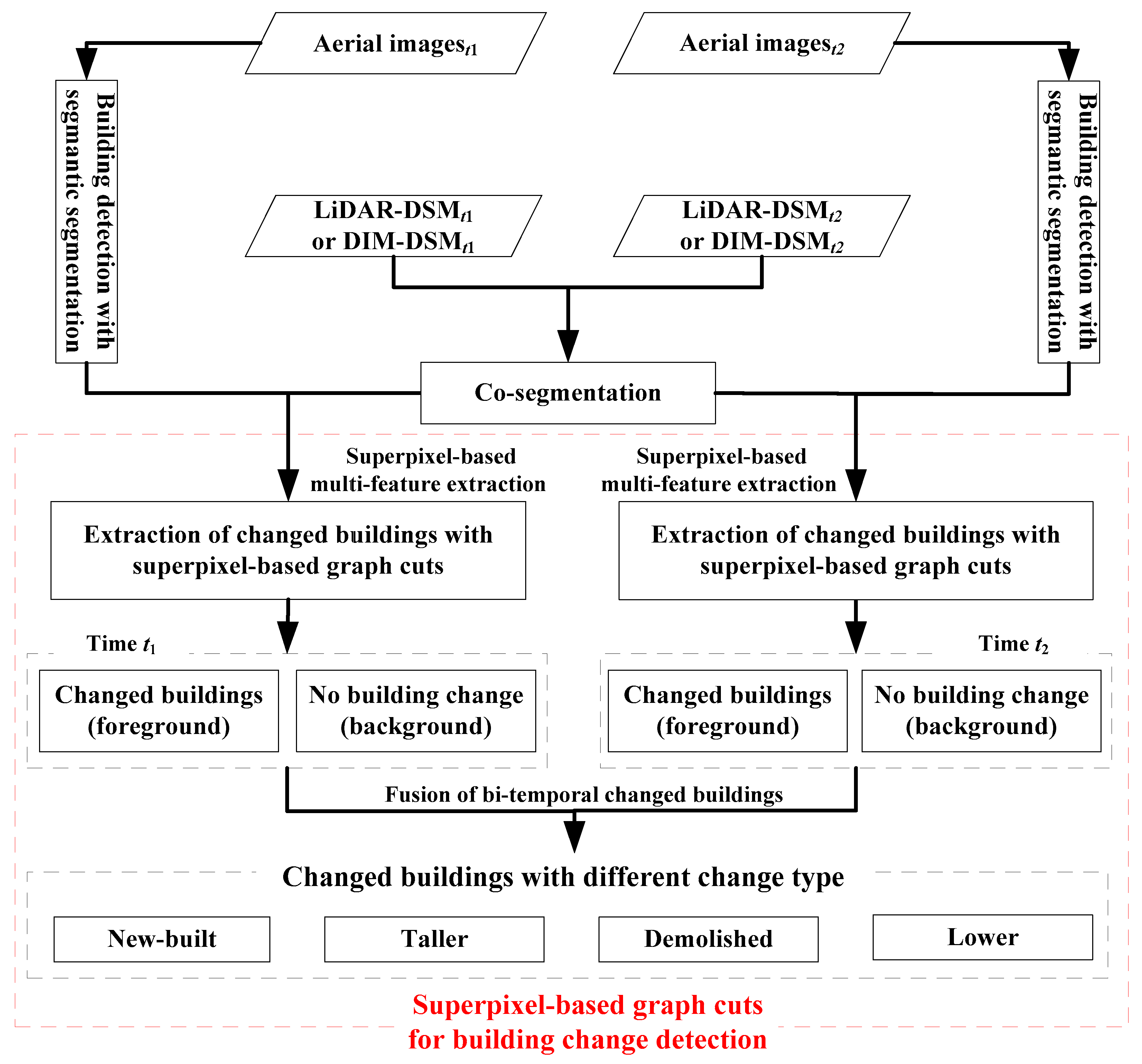
Article

Co-Segmentation and Superpixel-Based Graph Cuts for Building Change Detection from Bi-Temporal Digital Surface Models and Aerial Images

1
School of Educational Information Technology, Central China Normal University, Wuhan 430079, China
2
Collaborative Innovation Center of Geospatial Technology, Wuhan University, Wuhan 430079, China
3
School of Resource and Environmental Sciences, Wuhan University, Wuhan 430079, China
4
School of Remote Sensing and Information Engineering, Wuhan University, Wuhan 430079, China
5
Beijing Insititute of Surveying and Mapping, Beijing 100038, China
6
Beijing Key Laboratory of Urban Spatial Information Engineering, Beijing 100038, China
*
Author to whom correspondence should be addressed.
Submission received: 25 February 2019 / Revised: 19 March 2019 / Accepted: 23 March 2019 / Published: 26 March 2019
(This article belongs to the Special Issue Change Detection Using Multi-Source Remotely Sensed Imagery)

Abstract

:
Thanks to the recent development of laser scanner hardware and the technology of dense image matching (DIM), the acquisition of three-dimensional (3D) point cloud data has become increasingly convenient. However, how to effectively combine 3D point cloud data and images to realize accurate building change detection is still a hotspot in the field of photogrammetry and remote sensing. Therefore, with the bi-temporal aerial images and point cloud data obtained by airborne laser scanner (ALS) or DIM as the data source, a novel building change detection method combining co-segmentation and superpixel-based graph cuts is proposed in this paper. In this method, the bi-temporal point cloud data are firstly combined to achieve a co-segmentation to obtain bi-temporal superpixels with the simple linear iterative clustering (SLIC) algorithm. Secondly, for each period of aerial images, semantic segmentation based on a deep convolutional neural network is used to extract building areas, and this is the basis for subsequent superpixel feature extraction. Again, with the bi-temporal superpixel as the processing unit, a graph-cuts-based building change detection algorithm is proposed to extract the changed buildings. In this step, the building change detection problem is modeled as two binary classifications, and acquisition of each period’s changed buildings is a binary classification, in which the changed building is regarded as foreground and the other area as background. Then, the graph cuts algorithm is used to obtain the optimal solution. Next, by combining the bi-temporal changed buildings and digital surface models (DSMs), these changed buildings are further classified as “newly built,” “taller,” “demolished”, and “lower”. Finally, two typical datasets composed of bi-temporal aerial images and point cloud data obtained by ALS or DIM are used to validate the proposed method, and the experiments demonstrate the effectiveness and generality of the proposed algorithm.

1. Introduction

Building change detection, which is the process of identifying changed buildings through comparison and analysis of bi-temporal or multi-temporal high-resolution remote sensing data, plays an important role in geospatial information services including urban village renovation, identification of illegal or unauthorized buildings, and monitoring of urban growth. In previous years, some scholars [1,2,3,4,5,6,7,8] proposed detecting building changes from bi-temporal or multi-temporal high-resolution remote sensing imagery on the basis of spectral information alone. However, due to the factors of shadows, occlusions, relief displacement, and spectral variation of buildings, it is difficult to obtain highly accurate building changes and guarantee the reliability and stability of these methods. Owing to the breakthrough of laser scanner hardware and the technology of dense image matching (DIM), which can effectively obtain the digital surface model (DSM) and supply the robust height feature of buildings [9], an increasing number of scholars are studying 3D building change detection.
Following the category of 3D change detection proposed by Qin [10], current 3D building change detection can be divided into two categories: (1) Geometric comparison; and (2) Geometric-spectral analysis.
In terms of geometric comparison, some scholars proposed detecting building changes with height differencing [11,12,13,14] and projection-based differences [15]. In such methods, DSM is generally derived from an airborne laser scanner (ALS). The DSM obtained by ALS is accurate and reliable. These methods are easy to implement and have achieved promising results. However, due to the high cost of acquiring point cloud data by ALS, in most cases, there are no appropriate bi-temporal or multi-temporal ALS point cloud data available for building change detection, to some extent limiting the practicality of such methods.
On the other hand, some scholars proposed detecting building changes based on geometric-spectral analysis, and the main challenge of these methods is how to effectively integrate these two information sources into a 3D building change detection framework. According to different combinations, Qin [10] subdivided them into three ways: (1) Post-refinement, (2) Direct feature fusion, and (3) Post-classification.
In post-refinement, using multi-temporal aerial stereo pairs, Jung [16] first compared two DSMs to initially locate the changed areas and then classified the resulting regions of interest with decision trees to find changed buildings. Furthermore, Pang et al. [9] proposed a building change detection framework to extract changed buildings with different change types from bi-temporal dense-matching point cloud and aerial images. In this method, changed objects above ground were firstly extracted by graph cuts, then a structural feature extracted from an aerial image was constructed to classify the candidate changed building objects into building and non-building. Next, by combining bi-temporal classifications and DSMs, these changed building objects were further classified as “newly built,” “taller,” “demolished”, and “lower”. In such methods, parameters are easy to understand and tune, and the algorithms are flexible and efficient. These methods are suitable when the quality of the DSMs is good. However, when the DSM is of poor quality, the performance may worsen. Furthermore, the initial changes rely solely on the geometric comparison, and the false negative cannot be recovered in the subsequent steps [10].
In direct feature fusion, Tian et al. [17] proposed a region-based method for change detection by integrating the height and the radiometric differences of Cartosat-1 datasets into a weighted change vector analysis framework. A subsequent work in Tian et al. [18] adopted Dempster–Shafer fusion theory to combine height changes derived by DSM and the Kullback–Liebler divergence similarity measure between the original images to extract real building changes. In addition, rule-based classification [19,20,21], decision-tree [22], graph cuts [23], and random forest [24] were also used to fuse multiple features to achieve building change detection. These methods consider both geometric and spectral information at the same time, and in the algorithm framework it is easy to combine other information sources for change detection [10]. However, the parameter setting of the fusion algorithm in such methods is critical, and inappropriate parameter settings may cause errors in the final change detection.
In addition, considering that the bi-temporal or multi-temporal data may be from different sources or different shooting times, it is difficult to directly compare the geometry and texture between the two datasets. To this end, some scholars have proposed post-classification methods. Post-classification methods propose detecting objects of interest or performing land-cover classification before comparing the resulting labels (classes), which avoids direct comparison of the spectral and height information [10]. Qin et al. [25,26] proposed an object-based 3D building change detection from multi-temporal stereo images based on supervised classification. In this method, for each period of data, the Meanshift algorithm was firstly used to segment the object; secondly, features of the object were extracted and fed to the framework combining decision tree and Support Vector Machine (SVM) for supervised classification; finally, a comparative analysis was performed to achieve the change detection. In such methods, DSMs are usually aggregated into the classification or detection methods as an additional channel, and the proposed classification methods also include SVM [27], decision trees, and so on. Increasing 3D information can improve the accuracy of classification and object detection. Each period of data in the time series is classified independently, thus avoiding direct comparison of unrectified geometry and spectral features, and it is robust to the interference caused by different data sources or different acquisition conditions (different seasons, lighting, etc.). However, the change detection results of such methods usually depend on the classification accuracy. Single-phase classification errors may be accumulated in the final change detection results.
Strictly speaking, the proposed method belongs to the subclass of direct feature fusion in the second category. Moreover, since the datasets for building change detection involve bi-temporal high-resolution remote sensing data, the pixel-based method can easily produce salt and pepper noise and pixels are inappropriate processing units for building change detection. Three types of superpixel-based analysis units generated from different ways of segmentation have been proposed in remote sensing change detection studies: (1) image–object overlay, which is to segment one of the images in the time series to generate image–objects, and a simple overlay is made to other images for comparison; (2) image–object comparison, which is to segment each period of data in the time series independently; and (3) multi-temporal image–object, which is generated by segmenting the entire time series together [28]. The multi-temporal image–object considers all series of the data at the same time and it has a distinct advantage of minimizing sliver errors and potentially honoring key multi-temporal boundaries. Thus, in this paper, we propose segmenting the bi-temporal data together to generate bi-temporal superpixels (i.e., bi-temporal image–object), and the process is called co-segmentation in this paper. Then, on the basis of co-segmentation, the building change detection problem is converted into two binary classifications, and each period’s changed building extraction is a binary classification in which the changed building is the foreground and the other area is the background. Additionally, a superpixel-based graph cuts algorithm is designed to classify the superpixels into changed buildings or unchanged objects. Next, by fusion of the bi-temporal changed buildings and DSMs, the changed buildings are further classified as “newly built,” “taller,” “demolished”, and “lower”. Finally, two typical datasets composed of bi-temporal point cloud data and aerial images are used to verify the effectiveness and generality of the proposed method.
The main contribution of this paper lies in the following three aspects:
  • A novel co-segmentation algorithm is proposed to jointly segment bi-temporal DSMs into bi-temporal superpixels. The superpixels are consistent with both periods of high-resolution remote sensing data. It can effectively avoid salt and pepper noise and minimize sliver objects caused by segmentation of each period of data independently.
  • An effective superpixel-graph-cuts-based building change detection framework is proposed to extract changed buildings with different change types, in which bi-temporal superpixels are taken as the processing unit, building change detection is converted into binary classifications, and the graph cuts algorithm is used to achieve a global optimal solution with three-dimensional information and CNN-based semantic segmentation as the superpixel features.
  • The proposed framework is general and can be applied to point cloud data obtained by ALS and DIM. Different data sources (i.e., LiDAR-DSM and DIM-DSM) from the same region are used to validate the proposed method, which is of great significance to the selection of data sources in engineering practice.
The rest of this paper is organized as follows: Section 2 describes the proposed co-segmentation and superpixel-based graph cuts for building change detection, Section 3 presents the results, followed by the discussion in Section 4, and conclusions are drawn in Section 5.

2. Co-Segmentation and Superpixel-Based Graph Cuts for Building Change Detection

A novel building change detection framework based on co-segmentation and superpixel-based graph cuts from bi-temporal point cloud data and aerial images is proposed in this work, as shown in Figure 1. In this framework, bi-temporal aerial images and point cloud data obtained by ALS or DIM are taken as the input and changed buildings with the change types of “newly built”, “taller”, “demolished”, and “lower” are extracted as the output. This framework is composed of three parts: co-segmentation of bi-temporal DSMs (Section 2.1), building detection with semantic segmentation (Section 2.2), and superpixel-based graph cuts for building change detection (Section 2.3). The details are described from Section 2.1, Section 2.2 and Section 2.3.

2.1. Co-Segmentation of Bi-Temporal DSMs

For high-resolution remote sensing data, superpixels are considered to be the basic unit for change analysis. To obtain superpixels, several commonly used segmentation algorithms are available, such as simple linear iterative clustering (SLIC) [29], watershed [30], Meanshift [31], etc. The superpixels obtained by the SLIC algorithm have good consistency, compactness, and adherence to boundaries, and extension to supervoxel generation is straightforward [27]. Moreover, the data to be segmented in this paper involved different periods of data and multi-temporal image–object is considered to be the most appropriate analysis unit for change detection, thus, co-segmentation of bi-temporal DSMs is designed to obtain superpixels (i.e., bi-temporal image-object) with the SLIC algorithm in this paper.
Before the co-segmentation, gridded DSMs are firstly interpreted. The details of the interpolation are as follows: First, the points are assigned a grid index, and the grid size is set to a specific distance which is twice the space between neighbor points. Then, the median of points in each grid cell is selected as the value of the grid cell. With the same grid size, gridding is repeated on the bi-temporal point cloud to obtain gridded DSMt1 and DSMt2, respectively. To achieve the co-segmentation, bi-temporal gridded DSMs are combined, and the vector of each gridded point composed of bi-temporal coordinates and Lab color values can be expressed as [ x , y , z , z , l , a , b , l , a , b ] . A co-segmentation is performed on the combined gridded DSMs with the SLIC algorithm.
Herein, the co-segmentation process with the SLIC algorithm is similar to the traditional SLIC algorithm. The only difference is the distance measure D s . In addition, considering that the elevation change has an important impact on superpixel formation and subsequent change detection, a coefficient N H is added to the distance measure D s to adjust the impact of elevation change on superpixel formation. The corresponding D s is adjusted as follows:
{ d c = ( l j l i ) 2 + ( a j a i ) 2 + ( b j b i ) 2 + ( l j l i ) 2 + ( a j a i ) 2 + ( b j b i ) 2 d s = ( x j x i ) 2 + ( y j y i ) 2 d h = ( z j z i ) 2 + ( z j z i ) 2 D s = ( d c N C ) 2 + ( d s N S ) 2 + ( d h N H ) 2
where l i , a i , b i and l j , a j , b j are the Lab color value of the pixel i and the pixel j at Time t1; l i , a i , b i and l j , a j , b j are the Lab color value of the pixel i and the pixel j at Time t2, x i , y i and x j , y j are the column and row number of the grid of the pixel i and the pixel j . z i and z j are the height of the pixel i and the pixel j at Time t1; z i and z j are the height of the pixel i and the pixel j at Time t2. d c represents the color distance, d s represents the plane spatial distance, d h represents the height distance, and N S is the maximum spatial distance within the superpixel which is related to the minimum detected building area S. N C is the maximum color distance within the superpixel, and it is usually set to the range of [10.0–40.0]. N H is the maximum height distance within the superpixel, and it is set to 1.0 in this paper.
It should be pointed out that the proposed co-segmentation is also suitable for the point cloud data without RGB values. Their RGB values are assumed to be 0. The resulting co-segmentation of bi-temporal point cloud data with and without RGB is shown in Figure 2. From Figure 2, it can be seen that the superpixels obtained by the proposed co-segmentation are of good consistency and compactness, adhere to boundaries, and are consistent with bi-temporal datasets.

2.2. Building Detection with Semantic Segmentation

Deep learning has shown great potential in semantic segmentation and in object detection and classification, especially convolutional neural network (CNN)-based deep learning. Building detection in this paper also falls into this category, considering that the CNN-based dual multi-scale manifold ranking (DMSMR) network [32] is end-to-end, and this network utilizes dilated and non-dilated networks to jointly optimize the results. Furthermore, the network combined with multi-scale (MS), broader receptive field (Dilated) and manifold ranking optimization (MR-Opti) strategies enables training without additional aides. Thus, DMSMR network-based semantic segmentation is adopted in this paper to classify each pixel into one of the given categories, and the categories include “background”, “building”, “road”, “farmland”, “garden”, “woodland”, “grassland”, “structures”, “digging pile”, “desert”, and “waters”. More details about the training data (e.g., EvLab-SS Dataset) and model parameter settings can be seen in Reference [32]. In addition, it should be known that other CNN-based semantic segmentation algorithms for aerial images are also suitable for building detection in this paper.
In this paper, semantic segmentation is applied to the aerial images instead of the gridded RGB images. There are multiple classifications in the overlapping area, and inconsistencies may exist between different classifications. Thus, it is necessary to fuse the classification results of the overlapping area and the strategy of “winner takes all” is used as the law. Details of the fusion are as follows: (1) For each grid point P ( X , Y , Z ) , find the aerial images which contain this grid point; (2) Calculate the coordinates p i ( x i , y i ) of the grid point on each related aerial image S i according to the projection equation and obtain its corresponding classification, as shown in Figure 3; and (3) Fuse the classification of the grid point according to the law of “winner takes all”. That is to say, the most frequently occurring classification is taken as the classification of this grid point. Finally, (4) Traverse all the grid points to obtain the fused classification results of the entire region.
Considering that this paper focuses on building change detection, only the category of buildings is selected here, and all the other categories are assigned a value of 0. The gridded RGB image and its corresponding building detection with semantic segmentation at Time t1 can be seen in Figure 4.
The above building detection shown in Figure 4 is only an example for one period of building detection (i.e., Time t1). In this paper, the same processing, including semantic segmentation and fusion of the classification of grid points, needs to be performed on the bi-temporal aerial images separately and the building detections of bi-temporal grid points realized.

2.3. Superpixel-Based Graph Cuts for Building Change Detection

In this paper, the building change detection problem is converted into two binary classifications. For each period of data, with the bi-temporal superpixel as the processing unit, the extraction of changed buildings is a binary classification in which the changed buildings are the foreground and the other objects are the background, and a superpixel-based graph cuts algorithm is designed to achieve a global optimal solution. Next, by fusion of bi-temporal changed buildings and DSMs, the changed buildings are further classified as “newly built,” “taller,” “demolished”, and “lower”. After briefly introducing the overview of our superpixel-based graph cut, detailed extraction of changed buildings with superpixel-based graph cuts is described, followed by fusion of bi-temporal changed buildings.

2.3.1. Overview of Our Superpixel-Based Graph Cuts

For each period of data, extraction of the changed building is a graph-cuts-based binary classification, in which changed buildings are the foreground and the other objects are the background. The graph cuts algorithm which was initially proposed by Boykov et al. [33] is used to construct a weight map and the max-flow/min-cut algorithm [34] is adopted to find the optimal solution in this paper. The objective of the graph cuts algorithm is to assign a label (including foreground and background) to each superpixel by minimizing the following energy function E [34]:
E ( L ) = p P D p ( L p ) + ( p , q ) N V p , q ( L p , L q )
where L = { L p | p P } is the labels of all superpixels, and L p { f g , b g } represents the label of the superpixel p, in which ‘fg’ and ‘bg’ are abbreviations of foreground and background, respectively, corresponding to changed building objects and unchanged objects; P is the set of all superpixels (corresponding to nodes in the graph), D p ( L p ) represents the cost of assigning the label L p to the superpixel p. N is the set of all superpixel pairs in the neighborhood (corresponding to edges in the graph), p and q are two neighbor superpixels, and V p , q ( L p , L q ) defines the cost of assigning the labels L p and L q to the superpixel pair p and q. V p , q ( L p , L q ) encourages spatial coherence by penalizing discontinuities between neighboring superpixels. The key to the superpixel-based graph cuts for extraction of changed buildings is the energy definition including the data term and the smooth term, which will be introduced in the next section.

2.3.2. Extraction of the Changed Buildings with Superpixel-Based Graph Cuts

In this paper, the data term of graph cuts is calculated from multi-features of the superpixel. The multi-features contain the difference of DSM (dDSM), normalized DSM (nDSM), and the buildings detected by semantic segmentation. dDSM is mainly used to locate changed areas; meanwhile, nDSM and the buildings detected by semantic segmentation are combined to jointly extract the accurate buildings, so as to eliminate interference from non-buildings. For the data at Time t1, the data term is calculated as follows:
D p ( L p ) = { ( 1 C d D S M × C b l d _ t 1 ) , i f L p = f g C d D S M × C b l d _ t 1 , i f L p = b g
where C d D S M is calculated by dDSM, and C b l d _ t 1 is calculated by nDSM and the buildings detected by semantic segmentation at Time t1. Details are as follows:
C d D S M : The dDSM is derived from the difference of the bi-temporal gridded DSMs. The changed area has the characteristics of | d D S M | T 1 , and the threshold T 1 is determined by experience, which is set to the range of [1.0 m–1.5 m] in this paper. Furthermore, considering that the processing unit is the superpixel, for each superpixel, the C d D S M is calculated from the probability of the grid points with | d D S M | larger than T 1 , and C d D S M is calculated as follows:
C d D S M = T [ P R O | d D S M | T 1 > 0.5 ]
P R O | d D S M | T 1 = N u m | d D S M | T 1 N u m s p l
T [ x ] = { 1 , i f x i s t r u e 0 , i f x i s f a l s e
where P R O | d D S M | T 1 is the probability of the grid points with | d D S M | larger than T 1 in the superpixel, N u m | d D S M | T 1 is the number of grid points with | d D S M | T 1 in the superpixel, and N u m s p l is the total number of all grid points in the superpixel. The role of T function is to exclude some small errors.
C b l d _ t 1 : C b l d _ t 1 measures the probability of the superpixel belonging to the building class. The building detection with semantic segmentation can effectively extract buildings, as shown in Figure 4. However, in this paper, as the buildings were extracted by semantic segmentation using only two-dimensional spectral information, the utilization of 3D information is limited, and there are still a few errors, for example, the road in the rectangle of Figure 5 is misjudged as buildings. The nDSM which is obtained by subtracting DTM from the DSM can effectively refine these errors, as shown in Figure 5. Thus, it is necessary to further refine the building extractions obtained by semantic segmentation by combining the nDSM. In this paper, the nDSM is mainly used to exclude ground points from the building detection with semantic segmentation, and a filtering of point cloud data with harsh thresholds by the progressive TIN algorithm [35] is more inclined to obtain satisfactory results; in this process, the buildings are rarely misclassified as ground. Thus, in this paper, the building detection by semantic segmentation combined with the nDSM to extract buildings expressed as C b l d _ t 1 is as follows:
C b l d _ t 1 = T [ P R O c l a s s t 1 = b l d > 0.5 ] × T [ P R O n D S M t 1 T 2 > 0.5 ]
P R O c l a s s t 1 = b l d = N u m c l a s s t 1 = b l d N u m s p l
P R O n D S M t 1 T 2 = N u m n D S M t 1 T 2 N u m s p l
where the function T [ . ] is the same as the T [ . ] in Equation (6). P R O c l a s s t 1 = b l d represents the probability of the grid points classified as a building by semantic segmentation in superpixels at Time t1, and P R O n D S M t 1 T 2 represents the probability of the grid points with n D S M t 1 larger than T 2 in superpixels at Time t1. T 2 is the minimum building height determined by prior knowledge (i.e., 2.2 m). N u m c l a s s t 1 = b l d is the number of grid points classified as buildings in superpixels at Time t1, and N u m s p l is the total number of all grid points in superpixels. N u m n D S M t 1 T 2 is the number of grid points with n D S M t 1 T 2 in superpixels at Time t1.
For the smooth term, in addition to requiring that the labels between adjacent superpixels be as identical as possible, the average Z-value difference of the DSM between two neighbor superpixels is also considered, and the smooth term V p , q ( L p , L q ) is defined as:
V p , q ( L p , L q ) = { 0 i f   d L e n < T d L e n 1 or L p = L q d L e n T d L e n 1 T d L e n 2 T d L e n 1 β i f   T d L e n 1 d L e n < T d L e n 2 and L p L q β i f   d L e n T d L e n 2 and L p L q
d L e n = f a b s ( Z p ¯ Z q ¯ )
where d L e n is the absolute difference of the average Z-value of the D S M t 1 between two adjacent superpixels. Z p ¯ and Z q ¯ are the average Z-values of the D S M t 1 of the two adjacent superpixels p and q. The greater the difference, the greater the cost of the smooth term. T d L e n 1 and T d L e n 2 are minimum and maximum thresholds of the absolute difference of the superpixel-based average Z-value. In this study, T d L e n 1 and T d L e n 2 are set to 0.1 and 0.5 m, respectively. β is a scaling coefficient between the data term and the smooth term.
After the data term and the smooth term are defined, the minimum cut is obtained by the max-flow/min-cut algorithm and the superpixels are classified into changed building objects or other objects.
The changed building objects obtained by the above graph cuts are superpixel-based and a truly changed building may be divided into multiple superpixels. Thus, it is necessary to perform the post-processing of merging these superpixels to remove those small objects and interference. Details are as follows: First, connectivity is used to remove small objects with an area smaller than a defined threshold T S (e.g., 50 m2, which is set according to the specific task requirements). Then, for each changed object larger than the defined threshold, a region growing process [36] is used to form changed building objects and the growth criterion is based on the distance between two neighbor points. In this study, the distance threshold is set to 0.3–0.4 m. After the region growing process, the objects with a smooth area larger than half of the defined threshold are labelled as changed buildings. Next, traversing the superpixels, the superpixels composed of changed points greater than half are marked as changed, otherwise they are marked as unchanged.
The above processing is to obtain the changed buildings at Time t1. For extraction of the changed buildings at Time t2, the process is consistent with that of Time t1. The difference is that the extraction of the changed buildings at Time t1 with the superpixel-based graph cuts uses semantic segmentation, nDSM, and DSM at Time t1. Meanwhile, for the extraction of the changed buildings at Time t2, these corresponding data need to be replaced by semantic segmentation, nDSM, and DSM at Time t2. Details will not be repeated here. After the superpixel-based changed buildings at Time t2 are obtained, the same post-processing with the same threshold is performed to obtain the final changed buildings at Time t2.
The extraction of the changed buildings with superpixel-based graph cuts after post-processing at Time t1 and t2 is shown in Figure 6a,b.

2.3.3. Fusion of Bi-Temporal Changed Buildings

After obtaining the bi-temporal changed buildings with the above processing, these bi-temporal changed buildings are combined to further classify as “newly built”, “taller”, “demolished”, and “lower”. The rules are summarized as shown in Table 1.

3. Results

To verify the effectiveness and generality of the proposed algorithm, two datasets composed of bi-temporal point cloud data and aerial images are used for experiments. In this work, bi-temporal datasets were georeferenced and registered. The point cloud data can be obtained by ALS (i.e., LiDAR-DSM) or DIM (i.e., DIM-DSM) from the corresponding stereo aerial images. After a brief description of the datasets and accuracy assessment measures, the experimental results and evaluation of the proposed method are given below.

3.1. Description of Datasets

3.1.1. Dataset 1: Nanning

The first dataset is situated in Nanning, Guangxi Zhuang Autonomous Region, China. The size of this area is 1000 m × 1000 m. This area is a typical suburban area with sparse housing and dense farmland. There are also a few residential buildings surrounded by trees. An overview of the dataset and its enlarged subsets is shown in Figure 7. This dataset was composed of bi-temporal stereo aerial images acquired with the same type of camera and flight plans, and details including shooting time, camera, focal length, image size, pixel size, Ground Sample Distance (GSD), related number of images, forward lap, and side lap are shown in Table 2. The point cloud data (i.e., DIM-DSM) were generated by software inpho 6.0 from the stereo aerial images. The spacing between neighbor points was approximately 0.5 m. In this study, a software called TerraSolid was used to filter point cloud data (i.e., DIM-DTM). The parameters were as follows: max building size was set to 100 m, terrain angle was set to 88 degrees, iteration angle was set to 3 degrees, and iteration distance was set to 0.7 m.

3.1.2. Dataset 2: Guangzhou

The second dataset is situated in Guangzhou, Guangdong Province, China. The size of this area is 2000 m × 2000 m. This area is a complex urban scene including residential area with scattered dense buildings, industrial area with dense large buildings, suburban area with small buildings, residential area with buildings densely aligned along the street, and high-rise buildings, as shown in Figure 8. This dataset is composed of bi-temporal point cloud data acquired by airborne LiDAR Trimble 5700 and color images synchronously shot by a camera P65+, and details are shown in Table 3. The point density of the bi-temporal ALS data is 4 points/m2 to 6 points/m2. The ground points (i.e., LiDAR-DTM) are obtained by the commercial software named TerraSolid with the default parameters (i.e., max building size was set to 100 m, terrain angle was set to 88 degrees, iteration angle was set to 6 degrees, and iteration distance was set to 1.4 m). To compare the difference of building change detection between two different data sources (i.e., LiDAR-DSM and DIM-DSM), bi-temporal dense-matching point cloud data of this dataset were also generated by software inpho 6.0 from the corresponding stereo aerial images. The spacing between neighbor points was approximately 0.5 m, and the ground points (i.e., DIM-DTM) were extracted by TerraSolid with the same parameters as Dataset 1.

3.2. Accuracy Assessment Measures

In this paper, the ground truths are delineated manually. Three measures, including correctness (Cr), completeness (Cm), and quality (Q) derived from a confusion matrix are calculated to assess the accuracy of the proposed building change detection method. In the evaluation, the object is considered as the unit. As long as the changed object detected by the proposed method has an overlap with the ground truths larger than the minimum detected building area T S and the same change type as the ground truths, the detection is considered correct, otherwise it is considered incorrect. Considering that the building change detection has a different change type, a confusion matrix with different change types is recommended, as shown in Table 4. The correctness, completeness, and quality are defined as follows:
C o r r e c t n e s s = T P T P + F P 1 + F P
C o m p l e t e n e s s = T P T P + F N
Q u a l i t y = T P + T N T P + F N + F P 1 + F P + T N

3.3. Results and Evaluation

3.3.1. Evaluation of Semantic Segmentation

To better analyze the effect of building change detection, it is necessary to firstly analyze and evaluate the accuracy of semantic segmentation. Orthophotos, ground truth, the results, and corresponding evaluation of semantic segmentation of the two datasets are shown in Figure 9. There are four rows and four columns. Each row represents a set of semantic segmentation results and the left-to-right four figures are orthophoto, ground truth, semantic segmentation result, and result evaluation. The first and second rows are the semantic segmentation results of the Nanning dataset in 2011 and 2012, respectively. The third and fourth rows are the semantic segmentation results of the Guangzhou dataset in 2012 and 2013, respectively. Figure 9 shows that the semantic segmentation results are ideal and close to the ground truth. Compared to the Guangzhou dataset, the Nanning dataset has less salt and pepper noise. The false negatives (FNs) mainly occur on small buildings. The false positives (FPs) are mainly concentrated on bare land in building areas and some roads.
Their corresponding pixel-based statistics are shown in Table 5. The calculation of three measures are similar to the description in Section 3.2. Table 5 shows that compared to the Guangzhou dataset, the correctness and completeness of the Nanning dataset is worse. This is mainly attributed to the small number of buildings in this dataset. There is some bare land in building areas classified as buildings and some small buildings are misclassified as non-buildings. In terms of quality statistics, Nanning’s results are slightly better than Guangzhou’s.

3.3.2. Evaluation of Building Change Detection

In this section, two datasets, namely, the Nanning and Guangzhou datasets, are used to verify the effectiveness and generality of the proposed method. During the experiment, the parameters of the two datasets are the same, and they are as follows: the parameters of the co-segmentation are ( N S , N C , N H ) = ( 25 , 10 , 1.0 ) , the thresholds of the dDSM T 1 , nDSM T 2 , and minimum detected building area T S are 1.5 m, 2.2 m, and 50 m2, respectively. The scaling coefficient of the data term and smooth term of superpixel-based graph cuts β is set to 0.2; T L e n 1 and T L e n 2 are 0.1 m and 0.5 m, respectively.
A. Comparison with other methods
To verify the effectiveness of the proposed method, a comparison between the proposed method and the other three methods, namely the image-based post-classification method (e.g., SemanticDIF, which is the differencing of semantic segmentation), DSMDIF (DSM differencing) [13], and the post-refinement method [9], is performed over the Nanning dataset. The results and evaluations of the methods are shown in Figure 10. From Figure 10, it can be seen that the proposed method extracted more accurate changed buildings than the other methods. SemanticDIF uses only spectral information without 3D information. It is not able to detect the changed buildings with change types of “taller” and “lower”, which is the main reason for the FN in Figure 10f. DSMDIF detected a great deal of changes according to the elevation difference. However, much work is still needed to eliminate the salt and pepper noise and the disturbances caused by non-buildings. The post-refinement method extracted most changed buildings with the right change type. However, there still exist some FNs and FPs. Compared with the post-refinement method, the proposed method has less FPs. The results of the proposed method are consistent with the ground truth and it is proved that the proposed method is effective.
Table 6 shows the statistics of the comparison over the Nanning dataset. For pixel-based statistics, DSMDIF achieves the highest completeness, but it has the lowest accuracy and quality. The proposed method achieves the highest accuracy and quality. In terms of completeness, although SemanticDIF has many FNs, there is little difference from those achieved by Post-refinement and the proposed method (62.6% for Post-refinement and 64.0% for Proposed). The same is true in terms of quality. To this end, we add object-based statistics for Post-refinement and the proposed method, and object-based statistics is mainly used in the follow-up experiments.
For object-based statistics, correctness, completeness, and quality of the proposed method in the Nanning dataset are 92.9%, 96.8%, and 90.1%. Compared with the post-refinement method proposed in Reference [9] whose correctness, completeness, and quality of the dataset 1 are 88.6%, 98%, and 86.9%, respectively, there are some improvements in the correctness and the quality. This is mainly attributed to the semantic segmentation used in this paper which can accurately extract the building area. The FPs are mainly caused by errors in DSM for textureless areas and occlusion areas. However, there is a slight reduction in the completeness. This is mainly due to 3 FNs caused by wrong semantic segmentation (2/3) and nDSM (1/3). The biggest reason lies in the model of semantic segmentation in this paper which is a general model for most aerial and satellite image data (GSD range from 0.1–10.0 m). The 5 misclassified detections (e.g., FP1) are mainly attributed to the following aspects: errors in DSM caused by buildings under construction (2/5), wrong semantic segmentation (1/5), and small buildings whose smooth area is smaller than the area threshold (2/5), as shown in Figure 11.
B. Comparison from different data sources
To verify the generality of the proposed method and to guide the selection of data sources in engineering practice, dataset 2 covering very complex scenes composed of LiDAR-DSM and DIM-DSM is also selected for the result evaluation. Compared with the first Nanning dataset, the second Guangzhou dataset, where some buildings are scattered and dense and the streets are narrow, poses a great challenge to the building change detection. The results from LiDAR-DSM, the result evaluations, and object-based statistics of building change detection from two data sources are shown in Figure 12 and Figure 13 and Table 7.
Figure 12 shows that the proposed building change detection from bi-temporal LiDAR-DSMs and images is almost consistent with the ground truth. The FP is rare. This is mainly attributed to the proposed superpixel-based graph cuts with dDSM and CNN-based semantic segmentation combined with LiDAR-DTM, as the features presented in this paper can accurately detect changed buildings.
Figure 13 shows the results of proposed building change detection from two different data sources (i.e, LiDAR-DSM and DIM-DSM) in the same area. It can be seen that the proposed algorithm from two different data sources can obtain effective building change detections for the six selected areas. However, compared to the results from LiDAR-DSM, the results from DIM-DSM have more FPs for the residential areas with scattered dense buildings (A and F in Figure 13b). This is mainly due to the dense-image-matching errors in these areas, and more details will be explained in Discussion 4.1.
However, because of the complexity of dataset 2, there is still a small amount of FPs, FNs, and FP1, as shown in Table 7. For the LiDAR-DSM, the small amount of FPs is mainly caused by the following aspects: interference of suspected building objects (i.e., cars, sunshade), penetrating objects with two layers (i.e., skylight, roofs built with penetrating materials), interference of terrain change, as shown in Figure 14. Meanwhile, for the DIM-DSM, besides the above reasons, the errors caused by DIM and the filtering of point cloud data are the two biggest reasons, especially for the villages in the city (i.e., dense scattered building areas). Moreover, there are a few FNs and FP1s for dataset 2. The main reasons are as follows: broken roofs composed of several small roofs, small changed buildings sheltered by trees, and confused changed buildings, as shown in Figure 15.
C. Comparison between whether DTM data are included and different sources of DTM
To evaluate the necessity of DTM (i.e., the necessity of nDSM) for building change detection, comparisons are made between whether DTM data are included and different sources of DTM. The object-based statistics are shown in Table 8.
Table 8 shows that the existence of LiDAR-DTM can significantly improve the correctness, completeness, and quality of building change detection, from (75.6%, 92.4%, 71.2%) to (87.9%, 92.4%, 81.9%) for LiDAR and from (59.8%, 89.7%, 56.0%) to (70.7%, 89.8%, 65.4%) for DIM. However, for the existence of DIM-DTM, different scenarios may have different improvements. The correctness, completeness, and quality of dataset 1 are increased from (82.4%, 96.7%, 80.2%) to (92.9%, 96.8%, 90.1%), while the correctness, completeness, and quality of dataset 2 are increased from (59.8%, 89.7%, 56.0%) to (66.6%, 86.8%, 60.5%). This is mainly because the scene of Dataset 2 is more complicated, and Dataset 2 contains a large number of dense scattered buildings and narrow streets. There are no ground points in these areas, and the DIM-DTM may contain some errors. Therefore, for DIM-DTM, a certain degree of manual inspection and correction can improve and ensure the quality of building change detection.
In addition, it can also be seen from Table 8 that for the complex urban scenes, including dense scatter building areas (i.e., villages in the city) and narrow streets, the quality of building change detection from LiDAR-DSM is higher and more reliable than that from DIM-DSM. Meanwhile, for the suburban area, DIM-DSM-based building change detection is sufficient.

4. Discussion

4.1. Difference of LiDAR-DSM and Dense Image Matching Digital Surface Models (DIM-DSM)

To evaluate the difference between LiDAR-DSM and DIM-DSM, dataset 2 at Time t1 and t2 is used for statistics, and the overview and its enlarged subsets are shown in Figure 16. The corresponding histograms of difference of LiDAR-DSM and DIM-DSM are shown in Figure 17.
Figure 16 shows an overview at Time t1 and enlarged subsets of difference of LiDAR-DSM and DIM-DSM, and the corresponding orthophotos of dataset 2 at Time t1 and t2, and the large difference is concentrated in building boundaries, narrow streets between dense buildings, water areas, and vegetation areas. Corresponding histograms from Figure 17 show that the difference between the two data sources is mainly within a certain range (concentrated between [−0.27m ~1.28m] for t1 and [−0.14m~1.75m] for t2). These indicate that building change detection from DIM-DSM for general area should usually be sufficient. However, for the dense scattered building areas (i.e., villages in the city), DIM-DSM may contain some errors at Time t1 or t2 as shown in Figure 16 Area A and C, and these errors may result in FPs. Thus, for these areas, LiDAR-DSM may be more appropriate for building change detection with high precision requirements.

4.2. Parameter Selection

Taking into account the fact that the minimum height of detected building ( T 2 ) and the minimum area of detected building ( T S ) are related to engineering practice requirements, different minimum height of detected building and minimum area of detected building will have different ground truths. Thus, we only discuss the threshold of co-segmentation ( N S , N C , N H ) , threshold of dDSM T 1 , and scaling coefficient between the data term and the smooth term β. With dataset 2 (i.e., DIM-DSM) as an example, we fix several other items and change the item to be evaluated. The object-based statistics are shown in Figure 18. Figure 18a–d shows that the proposed method is insensitive to the changes of these four parameters ( N S , N C , N H , β ) . Figure 18e shows that when T 1 ranges from 0.5 to 2.5 m and ( N S , N C , N H , β ) = ( 0.5 S , 10 , 1.0 , 0.2 ) , T 1 = 1.5 achieves the optimal correctness, completeness, and quality of building change detection, thus we choose T 1 = 1.5 . ( N S , N C , N H , β , T 1 ) = ( 0.5 S , 10 , 1.0 , 0.2 , 1.5 ) is the optimal parameter for the proposed building change detection.

5. Conclusions

A novel building change detection framework based on co-segmentation and superpixel-based graph cuts from bi-temporal digital surface models and aerial images is proposed in this paper. In this method, bi-temporal superpixels are first obtained by the co-segmentation of bi-temporal DSMs with the SLIC algorithm. Then, for each period of data, with the dDSM, nDSM, and building semantic information as the features, changed buildings are extracted with the superpixel-based graph cuts. Next, by combination of the bi-temporal changed buildings and DSMs, these changed buildings are further classified as “newly built”, “taller”, ”demolished”, and “lower”. Finally, two typical datasets composed of DSM and aerial images are selected to verify the effectiveness and generality of the proposed algorithm. Extensive experiments show that the proposed building change detection algorithm is effective and general. It is suitable for both LiDAR-DSM and DIM-DSM. Two different data sources covering the same area show the significance of DTM and the different influence of DTM from different data sources on building change detection. Furthermore, different data sources also show their respective applicability for building change detection. This is important to guide the selection of data sources in engineering practice.
However, the proposed building change detection algorithm is related to semantic segmentation and DTM. The FN caused by semantic segmentation and DTM cannot be recovered in the subsequent graph cuts optimization. Furthermore, the post-processing of graph cuts algorithm operates under the assumption that the building roof is composed of a smooth area that is larger than a certain threshold. If the building roof is rough (e.g., the roofs with debris piled up), the proposed algorithm may fail.
The following should be noted: (1) our semantic segmentation only considers two-dimensional image spectral information, while the existence of accurate 3D information (e.g., LiDAR-nDSM) can effectively improve the accuracy of building detection and change detection, and (2) our building change detection framework is not an end-to-end CNN-based method. Therefore, in our future research, we will mainly focus on the following aspects: (1) a CNN-based semantic segmentation algorithm with LiDAR-nDSM added as a new channel; and (2) an end-to-end CNN-based change detection method.

Author Contributions

S.P. conceived and designed the experiments, and she also wrote the manuscript; X.H. guided the algorithm design and revised the manuscript; M.Z. realized the semantic segmentation. Z.C. guided the organization and writing of the manuscript, and he also revised the manuscript. F.L. aided the experimental verification and revised the manuscript.

Funding

This study was partially supported by National Natural Science Foundation of China (Project No. 41701389 and 41771363), the research funding by Guangzhou Science, Technology and Innovation Commission (Project No. 201802030008), China Postdoctoral Science Foundation funded project (Project No. 2016M602363), Beijing Postdoctoral Research Foundation (Project No. 2018046) and Funded by Beijing Key Laboratory of Urban Spatial Information Engineering (Project No. 2019208).

Acknowledgments

The authors would like to thank Guangzhou Jiantong Surveying, Mapping and Geoinfo Co., Ltd. for providing the Guangzhou dataset. The authors would like to thank Zhiqi Zuo for his work of data preparation including bi-temporal data registration and DSM generation. The authors would like to thank Kai Deng for his processing of semantic segmentation.

Conflicts of Interest

The authors declare no conflict of interest.

References

  1. Argialas, D.; Michailidou, S.; Tzotsos, A. Change detection of buildings in suburban areas from high resolution satellite data developed through object based image analysis. Surv. Rev. 2013, 45, 441–450. [Google Scholar] [CrossRef]
  2. Bouziani, M.; Goïta, K.; He, D.-C. Automatic change detection of buildings in urban environment from very high spatial resolution images using existing geodatabase and prior knowledge. ISPRS J. Photogramm. Remote Sens. 2010, 65, 143–153. [Google Scholar] [CrossRef]
  3. Huang, X.; Zhang, L.; Zhu, T. Building change detection from multitemporal high-resolution remotely sensed images based on a morphological building index. IEEE J. Sel. Top. Appl. Earth Obs. Remote Sens. 2014, 7, 105–115. [Google Scholar] [CrossRef]
  4. Li, P.; Xu, H.; Guo, J. Urban building damage detection from very high resolution imagery using ocsvm and spatial features. Int. J. Remote Sens. 2010, 31, 3393–3409. [Google Scholar] [CrossRef]
  5. Tang, Y.; Huang, X.; Zhang, L. Fault-tolerant building change detection from urban high-resolution remote sensing imagery. IEEE Geosci. Remote Sens. Lett. 2013, 10, 1060–1064. [Google Scholar] [CrossRef]
  6. Vu, T.T.; Ban, Y. Context-based mapping of damaged buildings from high-resolution optical satellite images. Int. J. Remote Sens. 2010, 31, 3411–3425. [Google Scholar] [CrossRef]
  7. Hou, B.; Wang, Y.; Liu, Q. A saliency guided semi-supervised building change detection method for high resolution remote sensing images. Sensors 2016, 16, 1377. [Google Scholar] [CrossRef]
  8. Sofina, N.; Ehlers, M. Building change detection using high resolution remotely sensed data and gis. IEEE J. Sel. Top. Appl. Earth Obs. Remote Sens. 2017, 9, 3430–3438. [Google Scholar] [CrossRef]
  9. Pang, S.; Hu, X.; Cai, Z.; Gong, J.; Zhang, M. Building change detection from bi-temporal dense-matching point clouds and aerial images. Sensors 2018, 18, 966. [Google Scholar] [CrossRef] [PubMed]
  10. Qin, R.; Tian, J.; Reinartz, P. 3d change detection—Approaches and applications. ISPRS J. Photogramm. Remote Sens. 2016, 122, 41–56. [Google Scholar] [CrossRef]
  11. Pang, S.; Hu, X.; Wang, Z.; Lu, Y. Object-based analysis of airborne lidar data for building change detection. Remote Sens. 2014, 6, 10733–10749. [Google Scholar] [CrossRef]
  12. Teo, T.-A.; Shih, T.-Y. Lidar-based change detection and change-type determination in urban areas. Int. J. Remote Sens. 2013, 34, 968–981. [Google Scholar] [CrossRef]
  13. Murakami, H.; Nakagawa, K.; Hasegawa, H.; Shibata, T.; Iwanami, E. Change detection of buildings using an airborne laser scanner. ISPRS J. Photogramm. Remote Sens. 1999, 54, 148–152. [Google Scholar] [CrossRef] [Green Version]
  14. Awrangjeb, M.; Gilani, S.; Siddiqui, F. An effective data-driven method for 3-d building roof reconstruction and robust change detection. Remote Sens. 2018, 10, 1512. [Google Scholar] [CrossRef]
  15. Qin, R.J. Change detection on lod 2 building models with very high resolution spaceborne stereo imagery. ISPRS J. Photogramm. Remote Sens. 2014, 96, 179–192. [Google Scholar] [CrossRef]
  16. Jung, F. Detecting building changes from multitemporal aerial stereopairs. ISPRS J. Photogramm. Remote Sens. 2004, 58, 187–201. [Google Scholar] [CrossRef]
  17. Tian, J.; Reinartz, P.; d’Angelo, P.; Ehlers, M. Region-based automatic building and forest change detection on cartosat-1 stereo imagery. ISPRS J. Photogramm. Remote Sens. 2013, 79, 226–239. [Google Scholar] [CrossRef]
  18. Tian, J.; Cui, S.; Reinartz, P. Building change detection based on satellite stereo imagery and digital surface models. IEEE Trans. Geosci. Remote Sens. 2014, 52, 406–417. [Google Scholar] [CrossRef]
  19. Tian, J.; Nielsen, A.A.; Reinartz, P. Building damage assessment after the earthquake in haiti using two post-event satellite stereo imagery and dsms. Int. J. Image Data Fusion 2013, 6, 155–169. [Google Scholar] [CrossRef]
  20. Tian, J.; Chaabouni-Chouayakh, H.; Reinartz, P. 3d Building Change Detection from High Resolution Spaceborne Stereo Imagery. In Proceedings of the International Workshop on Multi-Platform/Multi-Sensor Remote Sensing and Mapping, Xiamen, China, 10–12 January 2011; pp. 1–7. [Google Scholar]
  21. Wenzhuo, L.; Sun, K.; Li, D.; Bai, T.; Sui, H. A new approach to performing bundle adjustment for time series uav images 3d building change detection. Remote Sens. 2017, 9, 625. [Google Scholar]
  22. Qin, R. An object-based hierarchical method for change detection using unmanned aerial vehicle images. Remote Sens. 2014, 6, 7911–7932. [Google Scholar] [CrossRef]
  23. Du, S.; Zhang, Y.; Qin, R.; Yang, Z.; Zou, Z.; Tang, Y.; Fan, C. Building change detection using old aerial images and new lidar data. Remote Sens. 2016, 8, 1030. [Google Scholar] [CrossRef]
  24. Chen, B.; Chen, Z.; Deng, L.; Zhou, J.; Zhou, J. Building change detection with rgb-d map generated from uav images. Neurocomputing 2016, 208, 350–364. [Google Scholar] [CrossRef]
  25. Qin, R.; Tian, J.; Reinartz, P. Spatiotemporal inferences for use in building detection using series of very-high-resolution space-borne stereo images. Int. J. Remote Sens. 2016, 37, 3455–3476. [Google Scholar] [CrossRef]
  26. Qin, R.; Huang, X.; Gruen, A.; Schmitt, G. Object-based 3-d building change detection on multitemporal stereo images. IEEE J. Sel. Top. Appl. Earth Obs. Remote Sens. 2017, 8, 2125–2137. [Google Scholar] [CrossRef]
  27. Arozarena, A. Change detection of buildings from satellite imagery and lidar data. Int. J. Remote Sens. 2013, 34, 1652–1675. [Google Scholar]
  28. Tewkesbury, A.P.; Comber, A.J.; Tate, N.J.; Lamb, A.; Fisher, P.F. A critical synthesis of remotely sensed optical image change detection techniques. Remote Sens. Environ. 2015, 160, 1–14. [Google Scholar] [CrossRef] [Green Version]
  29. Achanta, R.; Shaji, A.; Smith, K.; Lucchi, A.; Fua, P.; Süsstrunk, S. Slic superpixels compared to state-of-the-art superpixel methods. IEEE Trans. Pattern Anal. Mach. Intell. 2012, 34, 2274–2282. [Google Scholar] [CrossRef]
  30. Beucher, S.; Mathmatique, C.D.M. The watershed transformation applied to image segmentation. Scanning Microsc. Suppl. 1991, 6, 299–314. [Google Scholar]
  31. Comaniciu, D.; Meer, P. Mean shift: A robust approach toward feature space analysis. IEEE Trans. Pattern Anal. Mach. Intell. 2002, 24, 603–619. [Google Scholar] [CrossRef]
  32. Zhang, M.; Hu, X.; Zhao, L.; Lv, Y.; Luo, M.; Pang, S. Learning dual multi-scale manifold ranking for semantic segmentation of high-resolution images. Remote Sens. 2017, 9, 500. [Google Scholar] [CrossRef]
  33. Boykov, Y. Interactive graph cuts for optimal boundary and region segmentation of objects in n-d images. ICCV 2001, 1, 105–112. [Google Scholar]
  34. Boykov, Y.; Kolmogorov, V. An experimental comparison of min-cut/max-flow algorithms for energy minimization in vision. IEEE Trans. Pattern Anal. Mach. Intell. 2004, 26, 1124–1137. [Google Scholar] [CrossRef] [PubMed]
  35. Axelsson, P. Dem generation from laser scanner data using adaptive tin models. Int. Arch. Photogramm. Remote Sens. 2000, 33, 110–117. [Google Scholar]
  36. Adams, R.; Bischof, L. Seeded region growing. IEEE Trans. Pattern Anal. Mach. Intell. 2002, 16, 641–647. [Google Scholar] [CrossRef]
Figure 1. Workflow of the proposed algorithm for building change detection from point cloud data and aerial images.
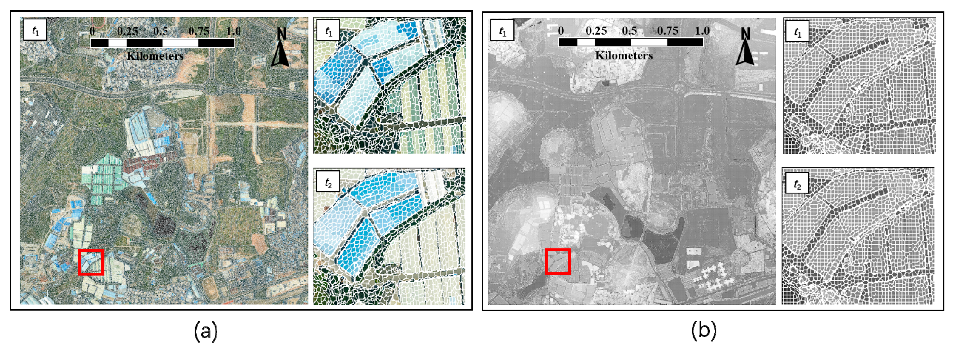
Remotesensing 11 00729 g001
Figure 2. Superposition of the co-segmentation and the gridded RGB images composed of RGB values of gridded color points at Time t1 and its enlarged subsets of the bi-temporal images. (a) Superposition of the co-segmentation and the gridded RGB image at Time t1, and the enlarged subsets of the bi-temporal modeled in the red rectangle; (b) Superposition of the co-segmentation and the gridded gray elevation image at Time t1, and the enlarged subsets of the bi-temporal gray elevation images in the red rectangle.
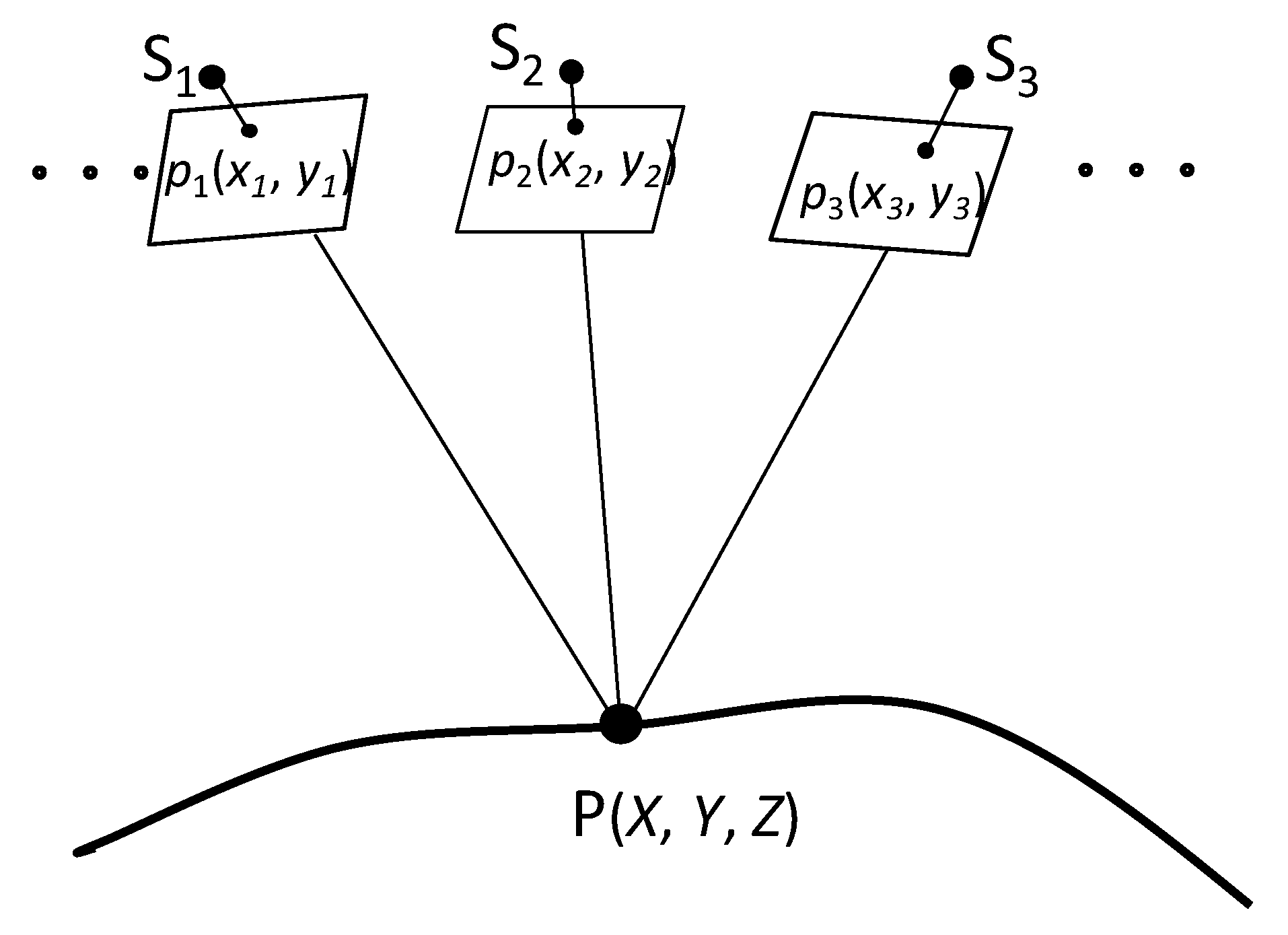
Remotesensing 11 00729 g002
Figure 3. An example of a grid point and its corresponding image points obtained by projection equation.
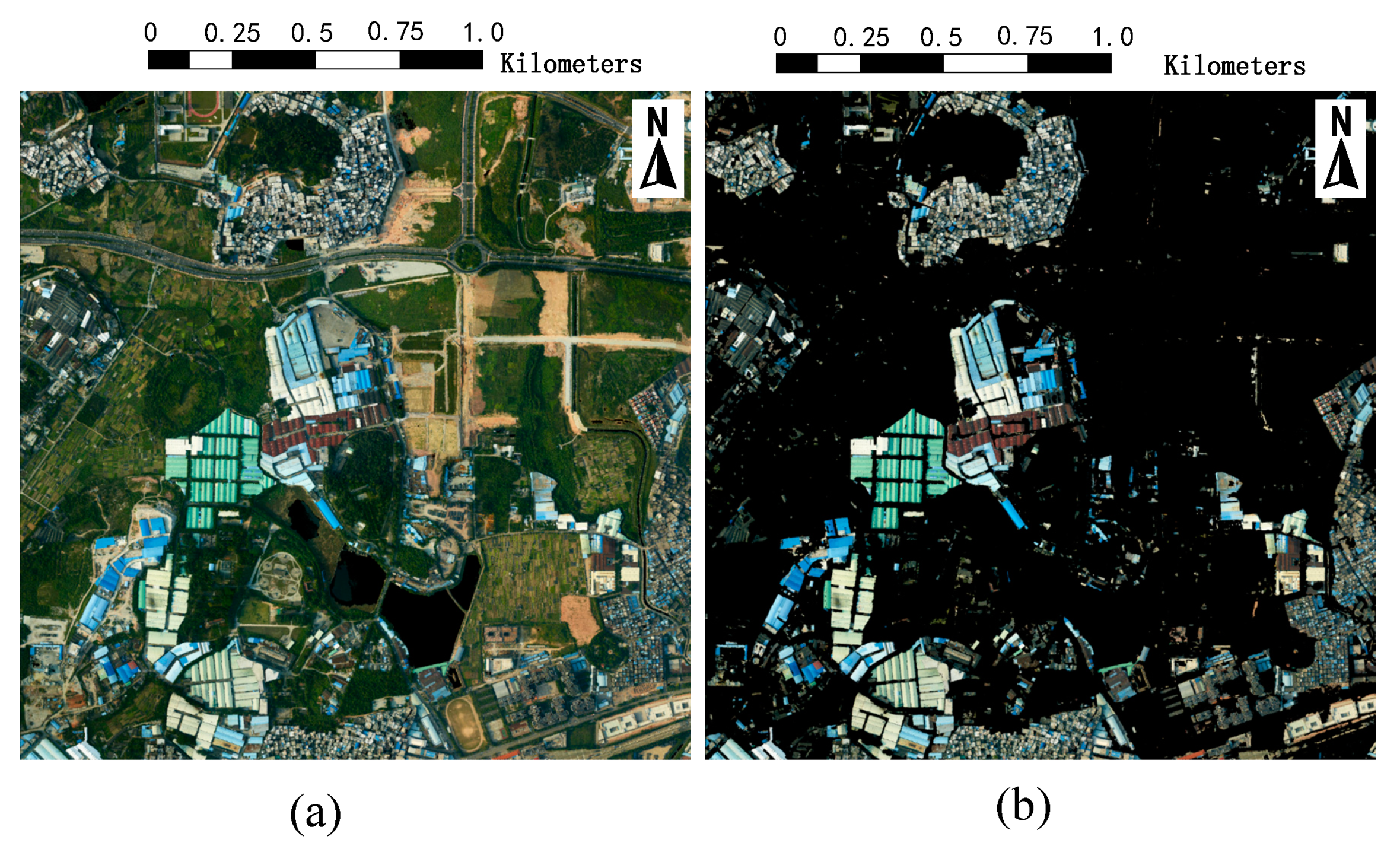
Remotesensing 11 00729 g003
Figure 4. The gridded RGB image and its corresponding building detection with semantic segmentation at Time t1. (a) The gridded RGB image; (b) Building detection with semantic segmentation.
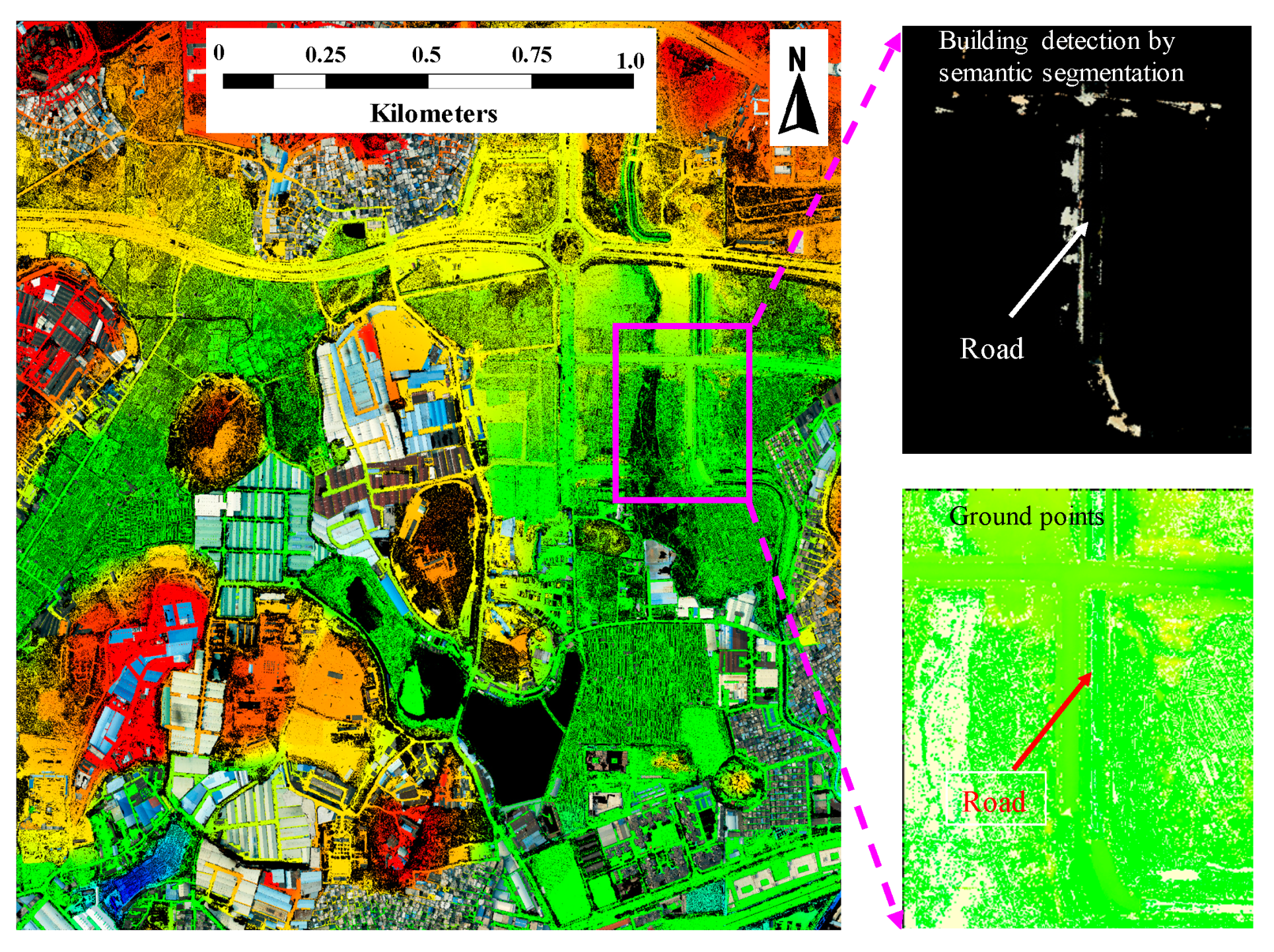
Remotesensing 11 00729 g004
Figure 5. Superposition of the building detection with semantic segmentation and the ground points from LiDAR-DSM, and its corresponding subsets of building detection and ground points.
Remotesensing 11 00729 g005
Figure 6. Extraction of the changed buildings at Time t1 and t2. (a) Extraction of the changed buildings at Time t1; (b) Extraction of the changed buildings at Time t2.
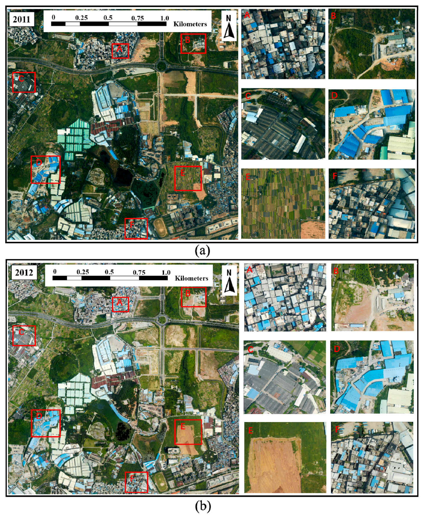
Remotesensing 11 00729 g006
Figure 7. Overview of the dataset 1 and its enlarged subsets. (a) Overview of the dataset 1 at Time t1 and its enlarged subsets; (b) Overview of the dataset 1 at Time t2 and its enlarged subsets.
Remotesensing 11 00729 g007
Figure 8. Overview of dataset 2 and its enlarged subsets. (a) Time t1; (b) Time t2.
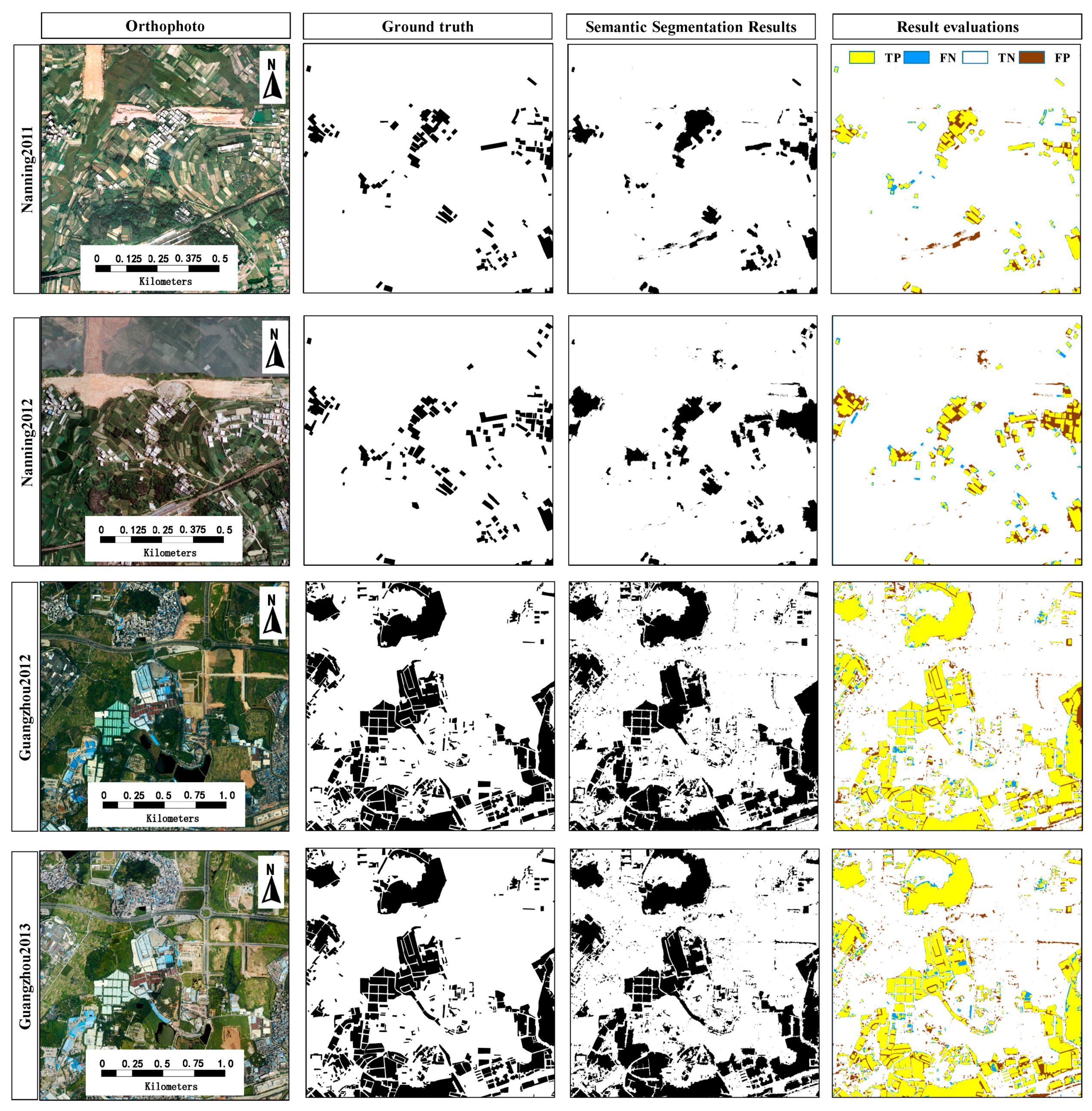
Remotesensing 11 00729 g008
Figure 9. Orthophotos, ground truth, semantic segmentation results, and result evaluations.
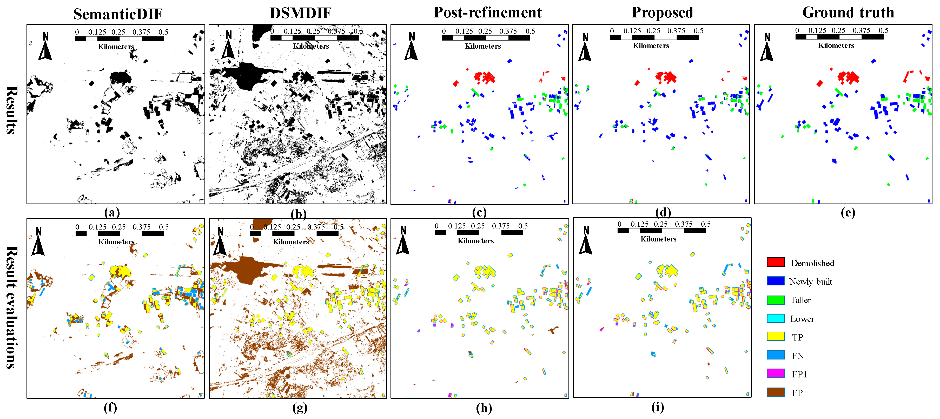
Remotesensing 11 00729 g009
Figure 10. Results and evaluations of the methods on the Nanning dataset. (ad) are the results of semantic differencing (SemanticDIF), digital surface model difference (DSMDIF), Post-refinement, and the proposed method, respectively; (e) is the ground truth of the Nanning dataset; (fi) are the result evaluations of SemanticDIF, DSMDIF, Post-refinement, and the proposed method, respectively.
Remotesensing 11 00729 g010
Figure 11. Examples of FN and FP1 of dataset 1. (a) FN caused by semantic segmentation at Time t1 and t2; (b) FN caused by normalized digital surface models (nDSM) at Time t1 and t2; (c) FP1 caused by errors in digital surface models (DSM) at Time t1 and t2; (d) FP1 caused by small buildings at Time t1 and t2.
Remotesensing 11 00729 g011
Figure 12. Ground truth and results of the proposed method of dataset 2. (a) Ground truth; (b) Results of the proposed method from bi-temporal LiDAR-DSMs and aerial images.
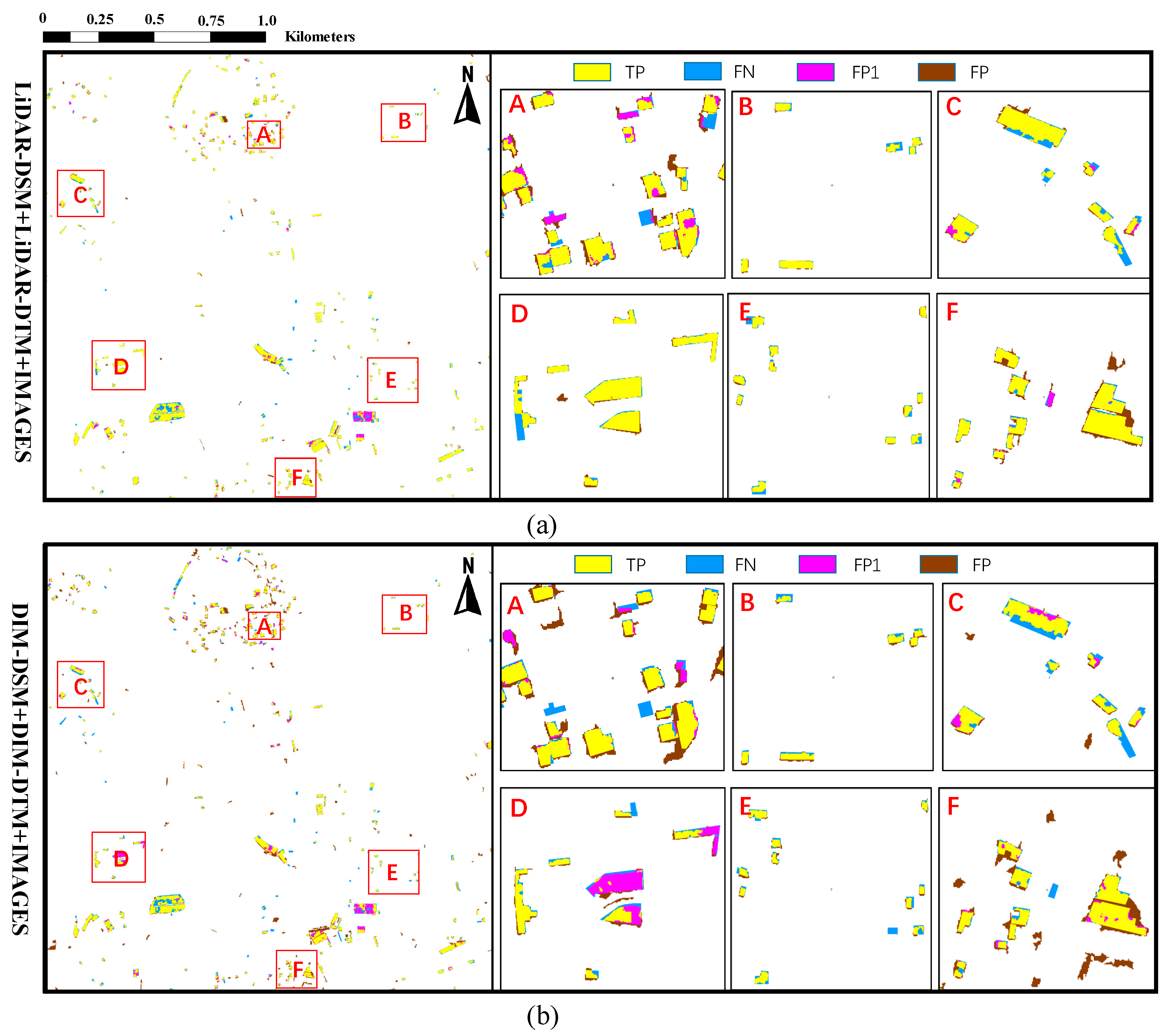
Remotesensing 11 00729 g012
Figure 13. Corresponding result evaluations of dataset 2 from LiDAR-DSM and dense image matching digital surface models (DIM-DSM). (a) Result evaluation from LiDAR-DSM and its enlarged subsets; (b) Result evaluation from DIM-DSM and its enlarged subsets.
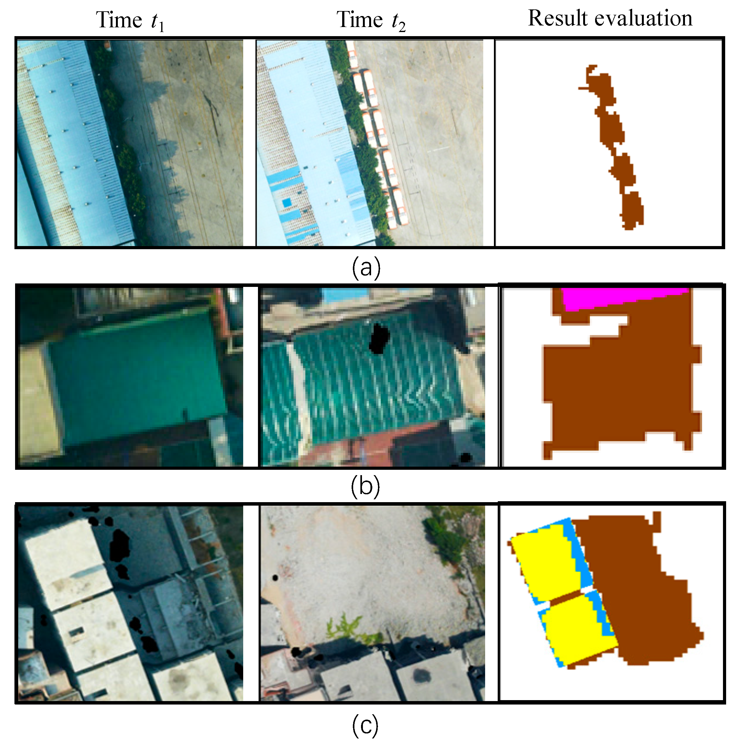
Remotesensing 11 00729 g013
Figure 14. Examples of FPs of dataset 2 from LiDAR-DSM. (a) FP caused by suspected building objects; (b) FP caused by penetrating objects; (c) FP caused by terrain change.
Remotesensing 11 00729 g014
Figure 15. Examples of FP1 and FN of dataset 2. (a) FP1 caused by broken roofs; (b) FN caused by small changed buildings sheltered by trees; (c) FN caused by confused changed buildings.
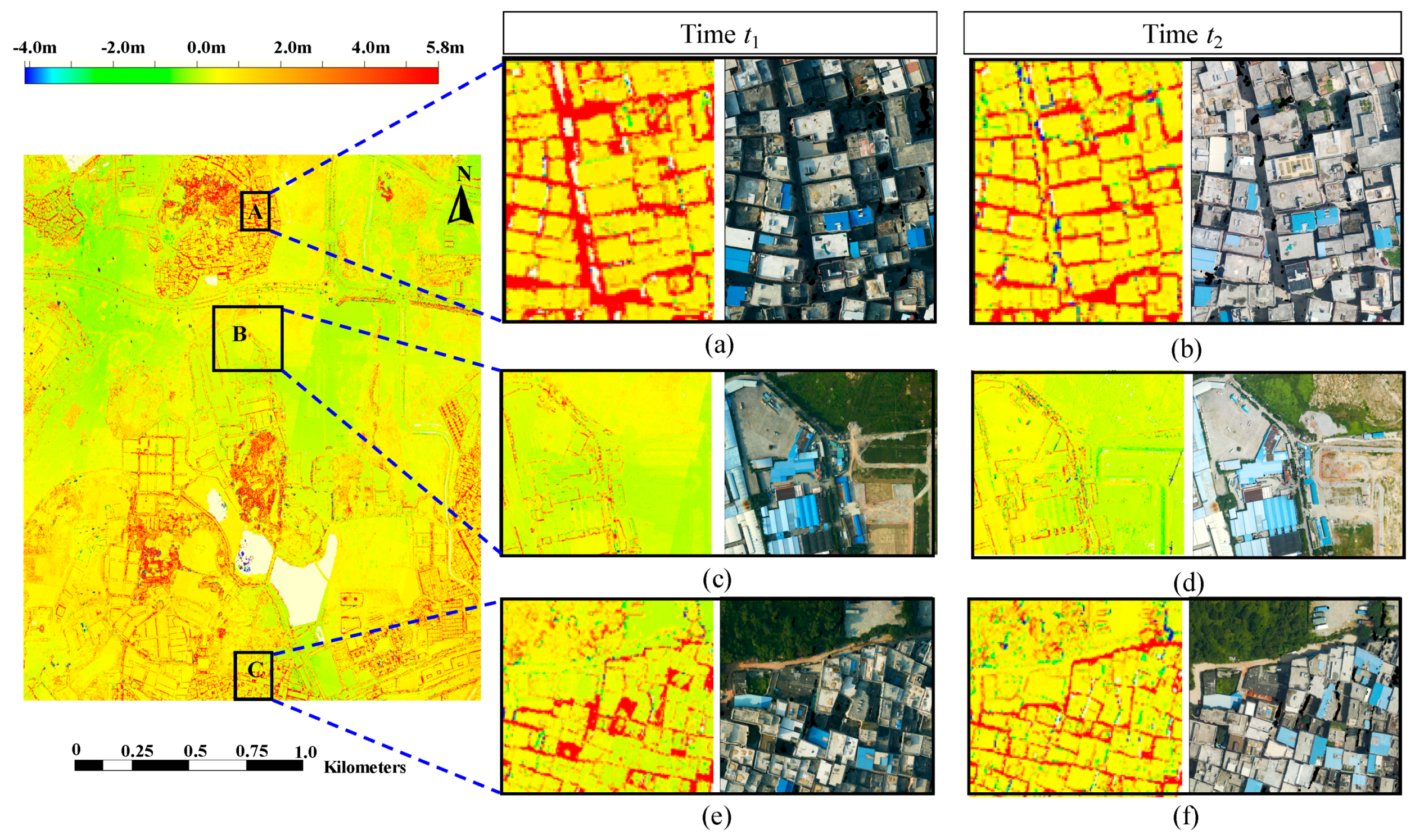
Remotesensing 11 00729 g015
Figure 16. Overview at Time t1 and enlarged subsets of difference of LiDAR-DSM and dense image matching digital surface models (DIM-DSM), and the corresponding orthophotos of dataset 2 at Time t1 and t2. (a) Enlarged subset of difference of LiDAR-DSM and DIM-DSM, and its corresponding orthophoto of area A at Time t1; (b) Enlarged subset of difference of LiDAR-DSM and DIM-DSM, and its corresponding orthophoto of area A at Time t2; (c) Enlarged subset of difference of LiDAR-DSM and DIM-DSM, and its corresponding orthophoto of area B at Time t1; (d) Enlarged subset of difference of LiDAR-DSM and DIM-DSM, and its corresponding orthophoto of area B at Time t2; (e) Enlarged subset of difference of LiDAR-DSM and DIM-DSM, and its corresponding orthophoto of area C at Time t1; (f) Enlarged subset of difference of LiDAR-DSM and DIM-DSM, and its corresponding orthophoto of area C at Time t2.
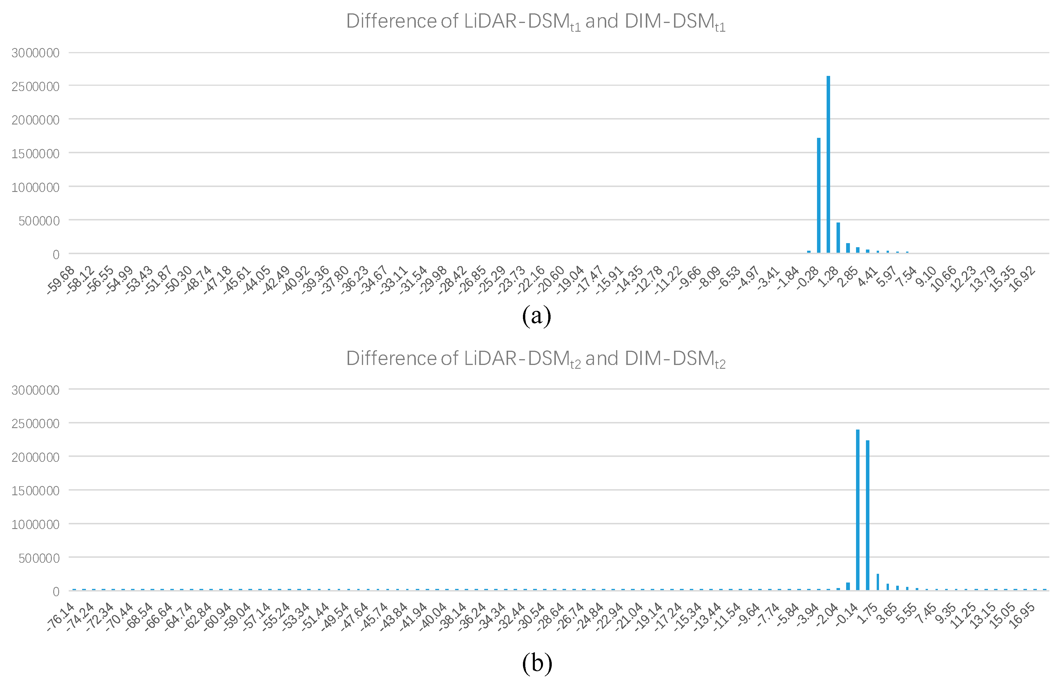
Remotesensing 11 00729 g016
Figure 17. Histograms of difference of LiDAR-DSM and dense image matching digital surface models (DIM-DSM) of dataset 2 at Time t1 and t2. (a) Histograms of difference of LiDAR-DSM and DIM-DSM of dataset 2 at Time t1; (b) Histograms of difference of LiDAR-DSM and DIM-DSM of dataset 2 at Time t2.
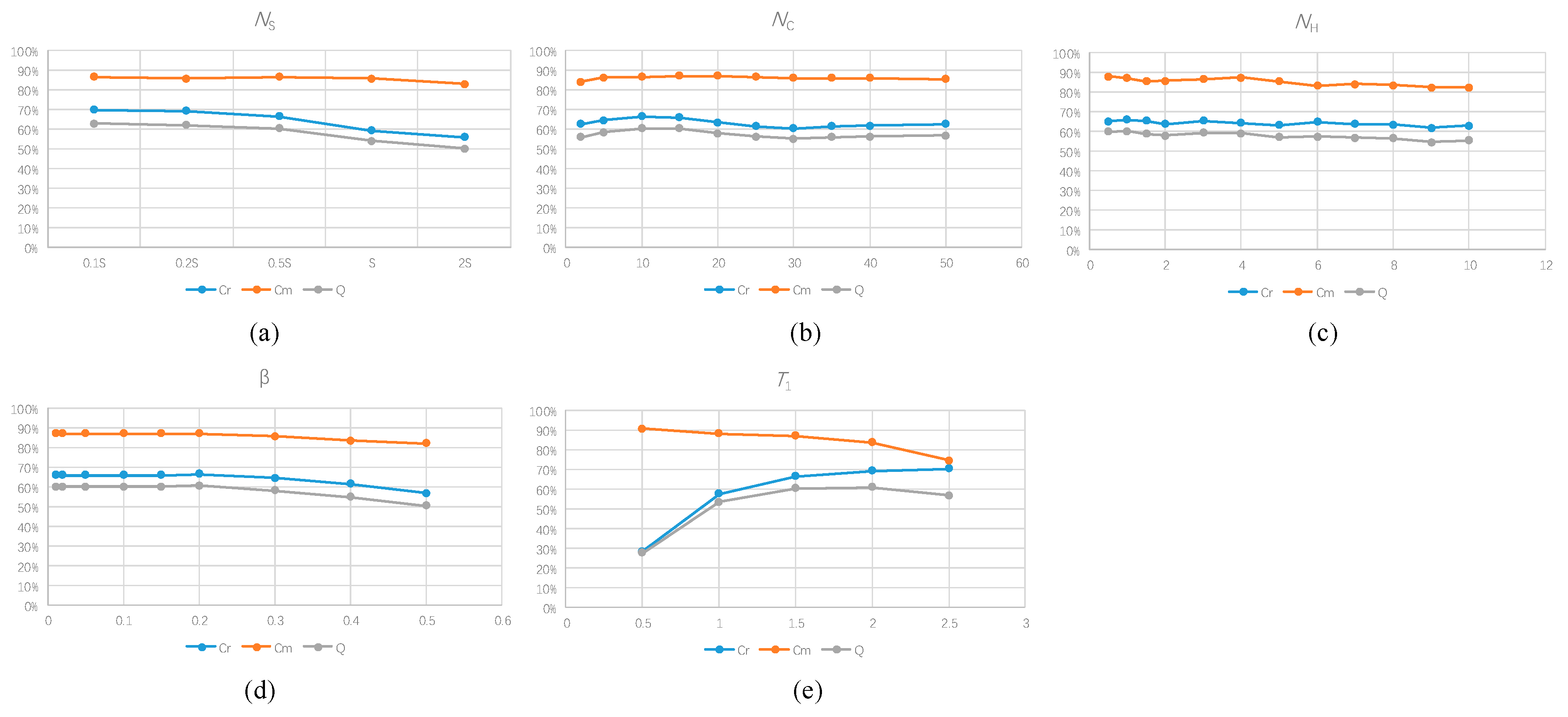
Remotesensing 11 00729 g017
Figure 18. Object-based statistics of building change detection with different parameters. (a) Object-based statistics of building change detection with ( N C , N H , β , T 1 ) = ( 10 , 1.0 , 0.2 , 1.5 ) and NS ranging from 0.1S to 2S; (b) Object-based statistics of building change detection with ( N S , N H , β , T 1 ) = ( 0.5 S , 1.0 , 0.2 , 1.5 ) and NC ranging from 2 to 50; (c) Object-based statistics of building change detection with ( N S , N C , β , T 1 ) = ( 0.5 S , 10 , 0.2 , 1.5 ) and NH ranging from 0.5 to 10; (d) Object-based statistics of building change detection with ( N S , N C , N H , T 1 ) = ( 0.5 S , 10 , 1.0 , 1.5 ) and β ranging from 0.01 to 0.5; (e) Object-based statistics of building change detection with ( N S , N C , N H , β ) = ( 0.5 S , 10 , 1.0 , 0.2 ) and T 1 ranging from 0.5 to 2.5.
Remotesensing 11 00729 g018
Table 1. Change type determination with the guidance of a priori knowledge.
Time t1/Time t2Changed BuildingNo Building Change
Changed BuildingTaller, if DSMt1 < DSMt2
Lower, if DSMt1 > DSMt2
Demolished
No building changeNewly builtNo building change
Table 2. Details of the bi-temporal stereo aerial images of dataset 1.
DatasetShooting TimeCameraFocal LengthImage SizePixel SizeGSDNumber of ImagesForward LapSide Lap
t12012DMC120 mm7680 × 13,82412 µm17 cm1065%35%
t22013DMC120 mm7680 × 13,82412 µm17 cm1065%35%
Table 3. Details of the bi-temporal stereo aerial images of dataset 2.
DatasetShooting TimeCameraFocal LengthImage SizePixel SizeGSDNumber of ImagesForward Lap
t1September 2011P65+52 mm5989 × 44889 µm13 cm5570%
t2August 2012P65+52 mm5989 × 44889 µm13 cm6670%
Table 4. Confusion matrix with different change types, where yellow represents true positive (TP), blue represents false negative (FN), rose and brown represent two types of false positive (e.g., FP1 and FP), and white represents true negative (TN).
Proposed\Ground TruthNo Building ChangeNewly Built TallerDemolishedLower
No building changeN11N12N13N14N15
Newly builtN21N22N23N24N25
TallerN31N32N33N34N35
DemolishedN41N42N43N44N45
LowerN51N52N53N54N55
Table 5. Pixel-based statistics of semantic segmentation of the two datasets.
DatasetsPixel-Based Statistics
CrCmQ
Nanning201173.8%87.2%97.7%
201262.4%83.3%95.7%
Guangzhou201282.1%92.4%93.2%
201381.0%90.9%92.3%
Table 6. Statistics of the comparison over the Nanning dataset.
MethodsPixel-Based StatisticsObject-Based Statistics
CrCmQCrCmQ
SemanticDIF37.0%62.8%94.6%---
DSMDIF17.9%86.0%84.8%---
Post-refinement61.2%62.6%97.6%88.6%98.0%86.9%
Proposed64.1%64.0%97.8%92.9%96.8%90.1%
Table 7. Confusion matrix of the building change detection in Dataset 2.
Proposed\Ground TruthNo Building ChangeNewly BuiltTallerDemolishedLower
LiDAR-DSM+LiDAR-DTM+IMAGESNo building change011190
Newly built12101900
Taller1010700
Demolished1101440
Lower10002
Dense image matching digital surface models (DIM-DSM)+ DIM-DTM+
IMAGES
No building change0194130
Newly built5290600
Taller6110500
Demolished4403400
Lower70002
Table 8. Object-based statistics of the proposed building change detection method in the two datasets.
Proposed\Ground TruthDataset 1Dataset 2
CrCmQCrCmQ
LiDARLiDAR-DSM+ LiDAR-DTM+IMAGES-87.9%92.4%81.9%
LiDAR-DSM+IMAGES-75.6%92.4%71.2%
DIMDense image matching digital surface models (DIM-DSM)+ LiDAR-DTM+IMAGES-70.7%89.8%65.4%
DIM-DSM+DIM-DTM+IMAGES92.9%96.8%90.1%66.6%86.8%60.5%
DIM-DSM+IMAGES82.4%96.7%80.2%59.8%89.7%56.0%

