Improving Aboveground Forest Biomass Maps: From High-Resolution to National Scale

Abstract

Forest aboveground biomass (AGB) estimation over large extents and high temporal resolution is crucial in managing Mediterranean forest ecosystems, which have been predicted to be very sensitive to climate change effects. Although many modeling procedures have been tested to assess forest AGB, most of them cover small areas and attain high accuracy in evaluations that are difficult to update and extrapolate without large uncertainties. In this study, focusing on the Region of Murcia in Spain (11,313 km²), we integrated forest AGB estimations, obtained from high-precision airborne laser scanning (ALS) data calibrated with plot-level ground-based measures and bio-geophysical spectral variables (eight different indices derived from MODIS computed at different temporal resolutions), as well as topographic factors as predictors. We used a quantile regression forest (QRF) to spatially predict biomass and the associated uncertainty. The fitted model produced a satisfactory performance (R² 0.71 and RMSE 9.99 t·ha⁻¹) with the normalized difference vegetation index (NDVI) as the main vegetation index, in combination with topographic variables as environmental drivers. An independent validation carried out over the final predicted biomass map showed a satisfactory statistically-robust model (R² 0.70 and RMSE 10.25 t·ha⁻¹), confirming its applicability at coarser resolutions.

1. Introduction

The Mediterranean basin represents a hotspot of biological diversity, being a socioecological system very sensitive to climate change effects [1]. A keystone concern is how to develop adaptive planning for the assessment, monitoring, and management of organic carbon in ecosystems, which is essential to achieve climate change commitments at a national level. Particularly in terrestrial ecosystems, forests play a basic role as carbon sinks containing about 80% of global terrestrial aboveground biomass (AGB). However, such information is difficult to produce, and the uncertainties about magnitude and location are often large [2,3]. Much of this uncertainty is due to the lack of detailed information about the spatial distribution of carbon stored in biomass. Thus, forest biomass is an important measure for environmental management to provide more insights into the amount and spatial distribution of carbon storage for supporting future climate change mitigation actions [4].

The use of light detection and ranging (LiDAR) technology aimed at studying forested ecosystems started in the 1970s, especially airborne laser scanning (ALS) systems. Airborne laser-based acquisitions have been extensively used in forestry inventories following area-based approaches, such as in AGB mapping [5,6,7]. This is due to ALS’s high sensitivity to structural features [8,9,10] and high precision ability to measure stand parameters in three dimensions previously calibrated with plot-level ground-based measures [11,12]. Moreover, several previous studies have proven the use of existing data sets, particularly national forest inventory plots, to be a feasible option to provide training data for stand-level ALS inventories (e.g., [13,14]). ALS data combined with machine learning modeling techniques are able to find substantial accuracy in forest biomass estimates at local scale [15,16]. Applications linking local and national—even global—scales allow the design of dynamic assessment and management planning, therefore increasing the accuracy and predictive capacity of global models predicting forest AGB. Despite technological advancement, the high cost of acquisition of ALS data results in much higher revisit time compared to satellite data, which reduces their continuous temporal and spatial availability, therefore making their use at national scale inoperative. Thus, ongoing efforts are needed to solve the challenges involved in integrating environmental assessment and management at concordant scales in order to address climate change at a national level [17].

In the last few years, different studies have integrated optical satellite data into different spatial and temporal resolutions for land surface monitoring in a highly operative way [18]. Satellite remote sensing technology is considered as the most effective approach to estimate biomass, since it provides adequate methods to produce a high-temporal characterization of vegetation attributes over spatially continuous large areas [19]. The information provided by the moderate resolution imaging spectroradiometer (MODIS) has been extensively applied to monitor forests at regional and large scales since 2010, therefore enabling the derivation of biophysical parameters which are highly valuable for forest management such as forest biomass [20,21]. MODIS offers a short revisit time, and the information acquired in several spectral bands can be summarized in different vegetation indices (VIs) that can be used as proxies of photosynthetic activity of vegetation [22]. The theoretical basis for empirical-based VIs is derived from typical spectral reflectance signatures of contrast between blue-red and near-infrared wavelengths’ response. This contrast can be quantified through the use of ratios, differences, weighted differences or linear band combinations [23]. Hence, a MODIS-based hypertemporal series of VIs allow to extract valuable information about vegetation phenology [24] and to estimate vegetation biomass [25]. On the one hand, the normalized difference vegetation index (NDVI) [26] has been widely used in many forestry applications. The NDVI is the ratio of contrasting reflectance between maximum absorption of red wavelength due to chlorophyll pigments and maximum reflectance of infrared wavelength owing to leaf cellular structure [27,28]. These characteristics have been highly correlated with green biomass, green leaf area index (LAI), and percent green vegetation cover [3,29]. Since forest biomass is conditioned by temporal dynamics, the annual profile of the NDVI time series can be considered as an indicator of seasonal dynamics of forest biomass. Furthermore, NDVI annual mean (as net primary production estimator) and its variation coefficient (as indicator of vegetation seasonality) are commonly used in forest biomass assessment [30]. On the other hand, NDVI shows saturation in dense and multilayered forest canopy [31]. Therefore, substantial efforts have been made to improve and develop new vegetation indices, such as the enhanced vegetation index (EVI), which is considered a modified NDVI. EVI improves sensitivity across regions with high biomass and shows a high vegetation monitoring capability through a decoupling of the canopy background signal with a reduction in atmospheric influences [32]. The soil adjusted vegetation index (SAVI) [33] was generated to minimize the soil reflectance effect. Additionally, Reference [34] noted that NDVI is limited by its nonlinear response, making it insensitive to differences at very low and high densities. Hence, other vegetation indices are considered more linearly related to biophysical parameters of vegetation, such as the renormalized difference vegetation index (RDVI) [35], which was developed to take combined advantage of the difference vegetation index (DVI = NIR – Red) [36] and the NDVI; and the modified simple ratio (MSR) [37], proposed over the RDVI because it shows more sensitivity to various biophysical parameters.

In combination with dynamic and easily updated remotely-sensed VIs, terrain variables have also been used in many studies predicting AGB as supplemental information aimed at increasing predictive power and statistical discrimination [38]. Since topography controls the main landscape processes related to structural characteristics of vegetation, such as water distribution and potential solar radiation [39], the digital elevation model (DEM) and the derivation of DEM-based predictor variables partially explain spatial patterns in AGB [40].

On the basis of the above, the use of high-resolution ALS data is a widely proven tool to collect and subsequently characterize structural forest stand attributes, with some limitations due to cost, revisit time, logistics, and data volumes involved in monitoring and mapping large areas [41]. Optical remote sensing data provide abundant and highly frequent observations to monitor extensive forest areas. However, coarse-resolution satellite data are often limited by the ground-based validation and nature of the measures, which can be largely insensitive to vertically distributed attributes [42]. The main hypothesis of this study is that there is a robust correlation between ALS-based forest AGB and VIs derived from MODIS data. Therefore, forest AGB spatial distribution can be estimated in those places were ALS information is not available. This study aimed to develop a methodological approach to improve nationwide assessment and mapping of AGB through combining high-resolution ALS data with hypertemporal and moderate-resolution satellite images in Mediterranean forests. A two-stage upscaling approach was applied where ALS-based forest AGB assessments, calibrated with plot-level ground-based measures, were used to train a machine learning method (quantile regression forest). Predictor variables consisted of MODIS–derived indices and topographic factors. As an approach of the estimation accuracy in the upscaling processes, the estimated variance of the AGB estimator was assessed according to Reference [43]. This methodology was mainly developed with open source software and always considering free available data.

2. Materials and Methods

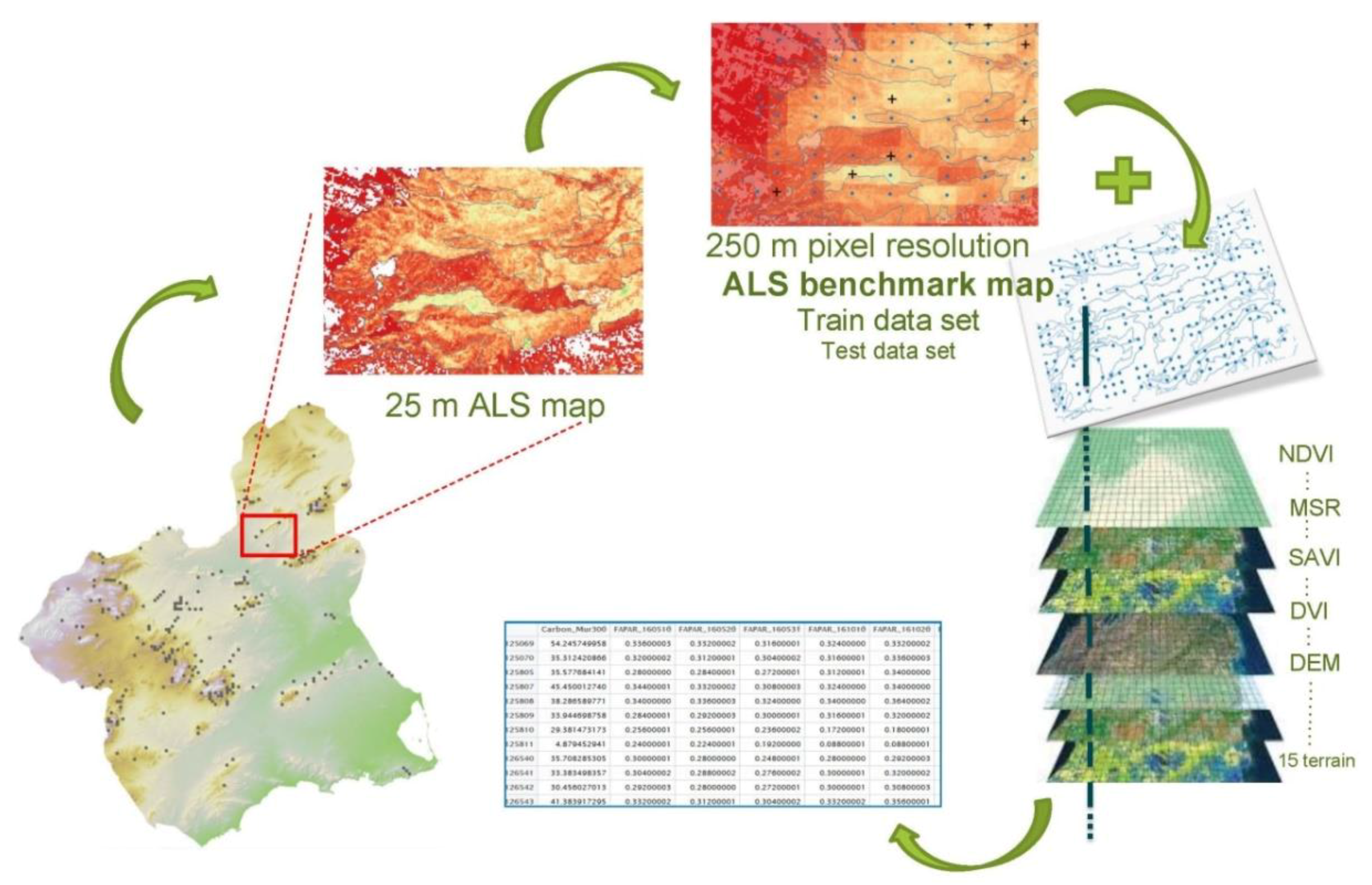
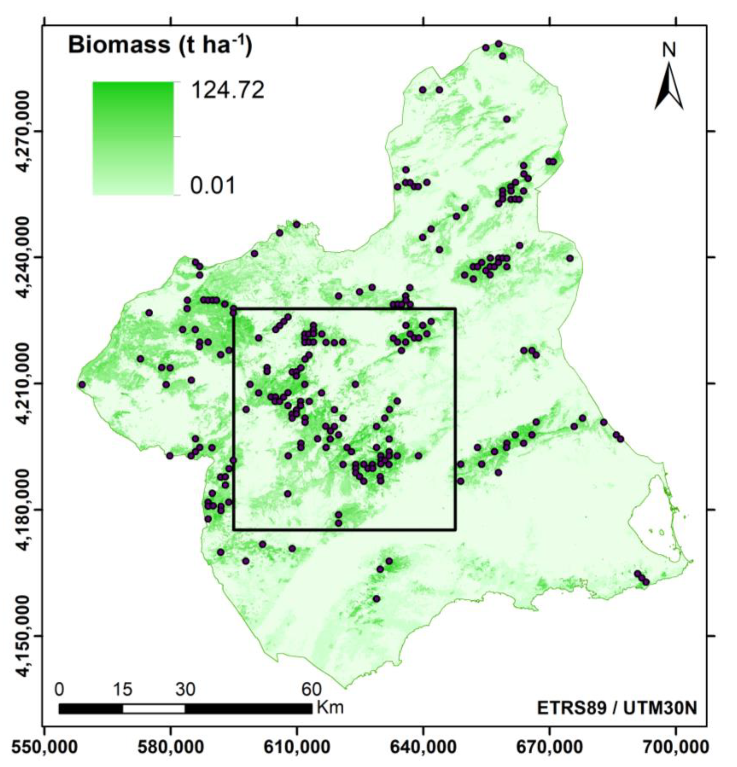
2.1. Study Area

Our study case was a Mediterranean region in Southeastern Iberian Peninsula (Region of Murcia), which is a particularly vulnerable area to global climate change threats due to its environmental characteristics [1]. The area is dominated by a dry, semiarid climate characterized by warm mean annual temperatures (ca. 18 °C), scarce annual rainfall (ca. 300–350 mm), and high mean annual evapotranspiration (ca. 900 mm) [44]. Climate variation is related to a diverse orography, which combines mountainous areas (up to 2000 m asl), high plateaus (500–1000 m), and badlands. The lithology is mainly represented by Calcisols, Leptosols, Regosols, and Fluvisols.

The combination of these environmental conditions shapes the land uses. Most of the Region of Murcia (11,313 km²) is highly influenced by human activity and, therefore, it is occupied by cultivated land. Fragmented forest areas represent approximately 45% of the study area. The wooded area is mostly composed of pine forest, Pinus halepensis Mill being the main species (ca. 90%) along with Pinus nigra Arn salzmanii and Pinus pinaster Ait, and holm oak (Quercus ilex L) to a lesser extent. That is to say, all the main species in this forest community are perennial. The shrubland area covers about of 60% of the forested area in the Region of Murcia.

2.2. From Field Plots to ALS Benchmark Map

2.2.1. Field Data

ALS plot-level biomass models were calibrated from the field plot database of the Fourth Spanish National Forest Inventory (SNFI) measured in 2010 in the Region of Murcia [45]. The SNFI is an extensive systematic survey carried out every 10 years on Spanish-forested areas on a basis of a regular network of 25 m radius plots at a density of 1 plot per km. From the complete database of the SNFI in Murcia (i.e., 1284 SNFI plots), a training dataset (i.e., 242 SNFI plots) was selected according to a stratified random sampling done within six predefined strata that covered the entire range of growing stock volume measures.

The main difficulty when using plots from the SNFI in combination with ALS data is the lack of precision in the plot center coordinates. Global navigation satellite system (GNSS) devices used in SNFI data collection, as other studies showed [46,47], have a nominal accuracy of 5–15 m. Following the methodology and the information sources proposed by Reference [48], the selected plots were relocated manually to improve the accuracy of the plot center coordinates. In this case, plots were shifted an average of 12.5 m in the relocation procedure.

The biomass model was based on four different information sources: (i) 2 m resolution ALS canopy models, (ii) sketches of plot location made by the field teams, (iii) high resolution orthoimagery from the Spanish National Plan for Aerial Orthophotography (PNOA in Spanish), and (iv) total height, species, and location of each measured tree in the field. The plot center relocation was intended to minimize possible errors derived from this lack of precision in the positioning of the plots. The SNFI plot size varies depending on tree diameter at breast height (dbh), that is to say, circular plots with four concentric subplots of a 5, 10, 15, and 25 m radius where trees with a dbh larger than 75, 125, 225, and 425 mm were respectively measured. In the SNFI, percent cover and mean height (in dm) were only estimated for each shrub species in the first plot radius (5 m).

In ALS-based forest inventories, the individual cell size of a grid that covers the entire study area has to be equal to the field plot size [49]. In this study, the selected SNFI plots were converted to plots with a maximum radius of 14.1 m (625 m²), in which we calculated forest AGB and extracted the ALS-derived metrics. Thus, only trees whose distance to the center of the SNFI plot was less than 14.1 m were taken into account to fit a maximum plot area equivalent to a 25 m × 25 m pixel. Therefore, the plots remained with only three concentric subplots of 5, 10, and 14.1 m. We calculated AGB for each selected SNFI plot as the sum of forest AGB related to each shrub species and single tree measured in these three subplots. AGB was scaled up to the hectare level according to the area of each subplot. Tree AGB was calculated through species-specific general models, reporting a goodness-of-fit (adj-R²) that was always higher than 0.95, as a function of dbh and total height [50]. To estimate shrub biomass, we applied a general model for Mediterranean shrublands (adj-R²: 0.63) that considers the shrub cover and its mean height as variables [51]. Grassland was excluded from the estimation due to ALS data inaccuracy to predict attributes related to this cover type.

Since SNFI data were collected over forested areas exclusively (i.e., forests and shrublands), we applied a forest mask to the study area based on the national forest map. The Spanish forest map (SFM) provides a detailed and updated version for the Region of Murcia at 1:25000 [45]. The SFM is the base cartography for the SNFI and describes the current distribution and seral stage of forest cover, based on structural and ecological descriptive items.

2.2.2. ALS Data Acquisition and Processing

ALS data were provided by PNOA. Data from two flight campaigns were used. A recent study demonstrated temporal transferability of pine forest attributes modeling by means of using low-density ALS data, even if data captured with different ALS instruments were considered [52]. In our case, data captured in the campaign of 2009 (one year before SNFI plot survey) were used to fit the aboveground biomass ALS model. ALS data captured in 2016–2017 were employed to implement the model and to obtain an updated prediction of forest biomass. Data from 2009 were captured from October to December 2009 using a Leica ALS50 system (Leica Geosystems AG, Heerbrugg, Switzerland) with a mean density of 0.5 pulse m⁻² and vertical RMSE ≤ 0.20. Data from 2016–2017 were captured from August 2016 to March 2017 using a Leica ALS60 system with a mean density of 0.7 pulse m⁻² and vertical RMSE ≤ 0.08. In both cases, ALS point cloud data were acquired in 2 × 2 km tiles covering the whole region, which were processed using the FUSION software [53].

Firstly, a 2 m resolution DEM was generated to subtract the orthometric elevation of the DEM from the z-coordinate of each ALS return aimed at normalizing the ALS point cloud. This procedure was applied separately to the ALS point cloud from each flight. Then, a normalized ALS point cloud of 2009 was used to compute a total of 15 metrics (

Table 1. Summary statistics of the response variable and the airborne laser scanning (ALS) metrics used for modeling in the set of Fourth Spanish National Forest Inventory (SNFI) plots (n = 242; 14.1 m from the plot center).

Group	Variable	Min	Max	Mean	SD
Response	Aboveground forest biomass (t·ha−1)	6.88	143.51	57.20	28.03
*ALS metrics	Hmean	2.75	13.34	6.38	1.98
	Hsd	0.55	4.86	1.99	0.73
	Hvar	0.30	23.61	4.49	3.55
	Hcv	0.16	0.50	0.31	0.06
	Hiq	0.76	8.13	2.90	1.15
	Hkur	1.43	4.77	2.51	0.56
	Hp01	2.02	5.00	2.39	0.52
	Hp05	2.04	6.97	3.07	1.00
	Hp10	2.06	8.06	3.66	1.28
	Hp25	2.27	10.94	4.93	1.73
	Hp50	2.48	14.00	6.44	2.17
	Hp75	3.10	17.64	7.83	2.45
	Hp90	3.51	19.24	8.94	2.67
	Hp95	3.77	19.59	9.50	2.78
	Hp99	4.24	20.15	10.25	2.94
	CRR	0.29	0.73	0.48	0.09
	TCC	1.88	93.86	44.55	19.87
	Hmean_LS	0.55	1.77	1.07	0.21
	TCC_LS	0.00	95.49	50.40	20.64

*ALS metrics: H = height of total returns above 2 m, sd = standard deviation, var = variance, cv = coefficient of variation, iq = interquartile range, kur = kurtosis, p = percentiles of total returns above 2 m, CRR = canopy relief ratio, TCC = tree canopy cover, Hmean_LS (low stratum) = mean height of the low stratum (total returns above 0.5 m and below 2 m), and TCC_LS = canopy cover of the low stratum.

) for each field plot using a threshold height of 2 m to separate trees from understory vegetation [54]. Amongst these considered metrics, tree canopy cover (TCC) refers to the ratio between the number of first returns above 2 m and the total number of first returns, whereas the canopy relief ratio (CRR) describes the relative canopy shape from altimetric observation [55]. CRR reflects the degree to which canopy surfaces are in the upper (>0.5) or lower (<0.5) portions of the height range [56]. Two other metrics of normalized ALS point cloud for each field plot were computed through filtering from the point cloud those points with a height lower than 2 m and using a height threshold of 0.5 m to separate shrubs from bare soil or herbaceous vegetation. These metrics correspond to mean height of the low stratum (Hmean_LS) and canopy cover of the low stratum (TCC_LS; i.e., the ratio between the number of first returns above 0.5 m and the total number of first returns).

Finally, the normalized ALS point cloud from 2016–2017 was used to compute the same set of metrics for the forest area in the entire region in 25 × 25 m pixels. We used this pixel resolution to reduce the impact on forest biomass scaling-up estimation and because this resolution is compatible with SNFI plot size.

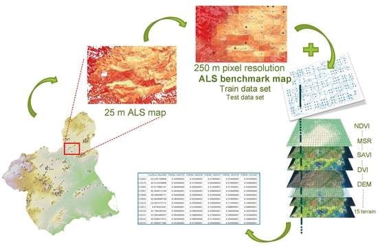
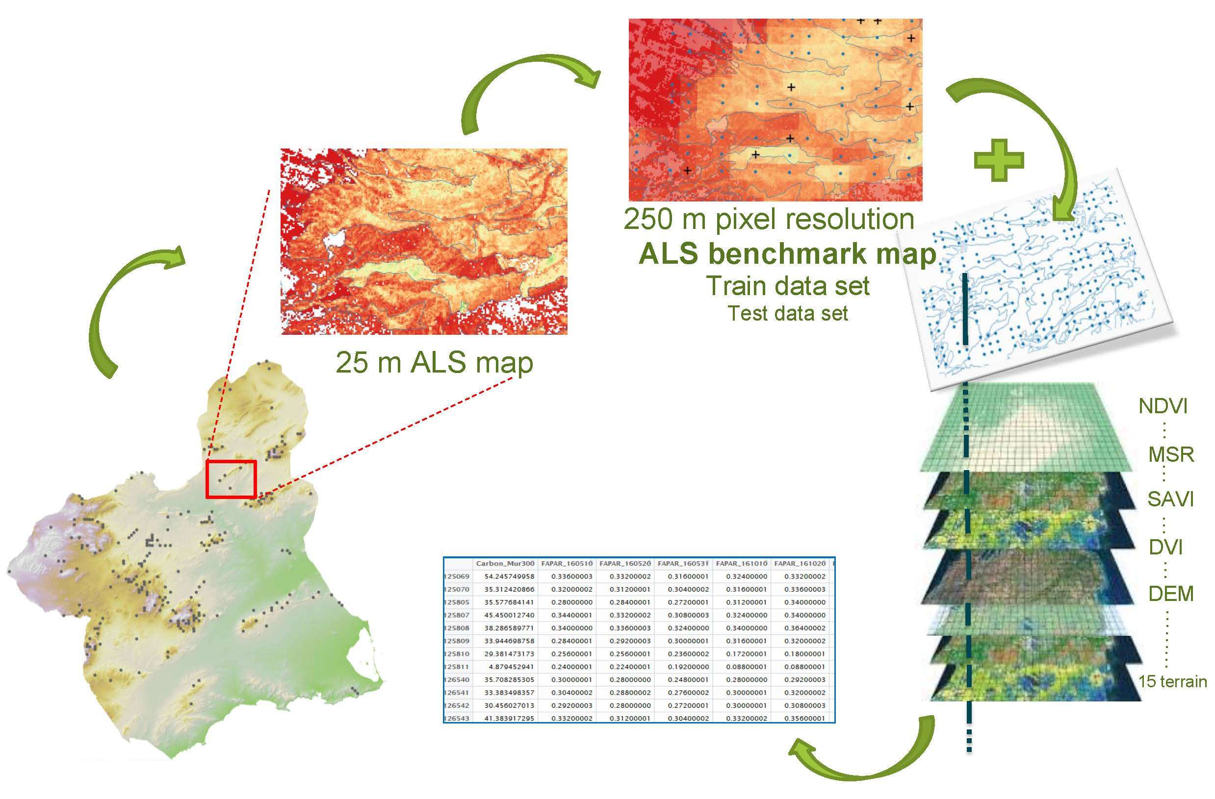
2.2.3. ALS Benchmark Map: Model, Spatial Prediction, and Resampling

The nonparametric regression algorithm random forest [57] was used to model the relationship between ALS-derived metrics with the ground-based measure of forest AGB computed from the SNFI plots (14.1 m radius). Analyses were carried out using the packages randomforest [58], VSURF [59], and rfUtilities [60] implemented in the R statistical software [61]. The VSURF package was applied to identify the combination of ALS metrics that best predicted forest AGB. This package provides an automated method to select predictor variables based on their importance scores while minimizing the redundancy among them. The out-of-bag error statistic provided in RF reports the goodness of model fit but not necessarily the predictive performance. For this reason, an independent data withholding of 10% was performed for a more precise model validation. A bootstrapping validation technique was followed by randomizing the independent data and executing the RF model a thousand times. Withheld data were predicted at each replicate. This cross-validation procedure was used by applying the random forest regression model cross-validation tool implemented in the rfUtilities package. Cross-validated estimates of root-mean-square error (RMSE) were calculated between the observed and predicted values using the training data. RMSE was normalized by the observations mean (RMSE%). The median percentage of explained variation (pseudo-R²) and RMSE% were reported for 1000 cross-validations.

The selected model was applied to the ALS metrics computed over the 2016–2017 point cloud covering forest area in 25 × 25 m pixel resolution. Therefore, a continuous 25 m ALS map of forest AGB in tons per hectare (t·ha⁻¹) was obtained. The resulting spatial cover was resampled to 250 m moderate resolution (MODIS variables resolution, see next subsection) using the bilinear method implemented in the resample package in R [62]. This ALS-based AGB map at 250 m pixel resolution was used as the forest AGB benchmark of the study area, henceforth ALS benchmark map.

2.3. From ALS Benchmark Map to MODIS Map

2.3.1. Optical Remote Sensing and Topographic Variables

A stack based on 1060 environmental predictors was generated according to dynamic and static variables. The dynamic variables refer to 8 VIs calculated using the newly release collection 6 of MOD09Q1 [63] and MOD13Q1 [23] MODIS products. These products respectively consist of 8-day and 16-day composites, both at 250 meters spatial resolution and corresponding to the closest dates to the 2016–2017 ALS data acquisition. Therefore, we obtained data for the years 2015, 2016, and 2017 from the Land Processes Distributed Active Archive Center (LP DAAC) [64]. Images were re-projected to the UTM zone 30, datum WGS-84 using the “MODIS Reprojection Tool” (MRT), and quality flags were decoded using the “Land Data Operational Products Evaluation” tool (LDOPE). Both tools were provided by the LP DAAC.

Several vegetation spectral indices were proposed as potential AGB estimators. We used red and near-infrared reflectance bands provided by the MOD09Q1 product to calculate the NDVI, MSR, DVI, RDVI, SAVI, and MSAVI, whereas near-infrared and short infrared reflectance values were used to calculate NDI7 (see equations in

Table 2. Equations of vegetation indices derived from moderate resolution imaging spectroradiometer (MODIS) data.

Vegetation Index	Equation 1
Normalized difference vegetation index (NDVI)	$NDVI=\frac{{\rho }_{NIR}-{\rho }_{RED}}{{\rho }_{NIR}+{\rho }_{RED}}$	[26]
Enhanced Vegetation Index (EVI)	$EVI=G·\frac{{\rho }_{NIR}-{\rho }_{RED}}{{\rho }_{NIR}+C_1·{\rho }_{RED}-C_2·{\rho }_{BLUE}+L}$	[32]
Normalized Difference Index 7 (NDI7)	$NDI7=\frac{{\rho }_{NIR}-{\rho }_{SWIR3}}{{\rho }_{NIR}+{\rho }_{SWIR3}}$	[65]
Modified Simple Ratio (MSR)	$MSR=\frac{\left(\raisebox{1ex}{${\rho }_{NIR}$}\!\left/ \!\raisebox{-1ex}{${\rho }_{RED}$}\right.\right)-1}{\sqrt{\raisebox{1ex}{${\rho }_{NIR}$}\!\left/ \!\raisebox{-1ex}{${\rho }_{RED}$}\right.}+1}$	[37]
Difference vegetation index (DVI)	$DVI={\rho }_{NIR}-{\rho }_{RED}$	[36]
Renormalized difference vegetation index (RDVI)	$RDVI=\frac{{\rho }_{NIR}-{\rho }_{RED}}{\sqrt{{\rho }_{NIR}+{\rho }_{RED}}}$	[35]
Soil adjusted vegetation index (SAVI)	$SAVI=\frac{\left({\rho }_{NIR}-{\rho }_{RED}\right)·\left(1+L\right)}{{\rho }_{NIR}+{\rho }_{RED}+L}$	[33]
Modified soil adjusted vegetation index (MSAVI)	$MSAVI=0.5·(2{\rho }_{NIR}+2-\sqrt{{\left(2{\rho }_{NIR}+1\right)}^2-8\left({\rho }_{NIR}-{\rho }_{RED}\right)})$	[66]

¹ρR, ρNIR and ρSWIR3 respectively correspond to the reflectance in the red (620–670 nm), near-infrared (841–876 nm), and shortwave infrared (2105–2155 nm) wavelengths. In SAVI, the accommodation coefficient of the soil background is L = 0.5, related to moderate canopy cover areas. In EVI, the canopy background adjustment for correcting the nonlinear is L = 1; the coefficients of the aerosol resistance term—which use the blue band to correct for aerosol influences in the red band—are C1 = 6 and C2 = 7.5, and the gain or scaling factor is G = 2.5.

). Time series were filtered in order to avoid abnormal values caused by clouds and certain atmospheric conditions. Low-quality pixel values were removed based on MODIS quality data bands and replaced by the average of the previous and subsequent date values with good quality in the time series. A smooth filter was also applied to remove outliers that fall outside the mean plus/minus two times the standard deviation within a five-date period window. The anomalous values were also replaced by the average of the previous and subsequent date values in the time series. In addition, time series from the MOD09Q1 product were smoothed with a Savitzky–Golay filter using a window width of 11 observations.

Reflectance bands were compiled, and indices were computed using the Environment for Visualizing Images (ENVI 4.5) software.

The properties of the VIs time-series can be summarized as ecologically relevant measures in a variety of indices [67]. Different variables derived from MODIS VIs time series were estimated to characterize seasonal dynamics of forest biomass in different time frames. To obtain the annual mean profile of each VIs, the 8-day and 16-day composites were layer-stacked to respectively create a 46- and a 23-band image for each year. We calculated the annual profile as the mean corresponding values of the three years considered (2015–2017).

In order to assess the maximum VIs values related to the growing season, for the 8-day composite of the 2015–2017 time period, we generated aggregates for the computed VIs (Table 2) time series using the maximum-value composite (MVC) approach [68]. The assumption behind the MVC technique is that the maximum NDVI value of a set of images will correspond to the ideal atmospheric and vegetation conditions. For the remaining VIs, the value corresponding to the date of the maximum NDVI value was selected.

As long-term ecosystem functioning descriptors, we calculated two variables from the 2001–2016 NDVI time series of the MOD13Q1 product: NDVI mean, as annual primary production prediction factor, and its standard deviation (NDVI sd) as the coefficient of seasonal variation, the latter being an indicator of vegetation seasonality [31]. Both variables were calculated according to the method described in [30].

According to [39,69], a local digital elevation model (DEM) was used to derive the static variables describing the topography to inform models with locally relevant information on landscape position. These static variables were 17 topographic parameters (

Table 3. Initial covariates used in the aboveground biomass predictive model from the airborne laser scanning (ALS) benchmark map to the MODIS map.

Covariate		Description (Time Period)	Product
Dynamic 1	NDVI MSR DVI RDVI SAVI MSAVI	8-day composite time series (2015–2017)	MOD09Q1
		8-day composite mean annual profile (2015–2017)
		Maximum-value composite (2015–2017)
	NDVI EVI NDI7	16-day composite time series (2015–2017)	MOD13Q1
		16-day composite mean annual profile (2015–2017)
	NDVI mean	Mean value (2001–2016)	MOD13Q1
	NDVI sd	Standard deviation (2001–2016)
Static	Topographic	Digital elevation model (DEM), analytical hillshading, slope, aspect, cross-section curvature, longitudinal curvature, convergence index, closed depressions, catchment area, topographic wetness index, Ls factor, channel network base level, vertical distance to channel network, valley depth, relative slope position, multiresolution valley bottom flatness index, multiresolution ridge top flatness index.	Terrain Analyst function in SAGA GIS software

¹ Normalized difference vegetation index (NDVI), enhanced vegetation index (EVI), normalized difference index 7 (NDI7), modified simple ratio (MSR), difference vegetation index (DVI), renormalized difference vegetation index (RDVI), soil adjusted vegetation index (SAVI), modified soil adjusted vegetation index (MSAVI).

) derived from a 25 m DEM, which is available at the Centre of Spanish National Geographic Institute (IGN). The current DEM version was generated by the IGN from ALS data interpolation. We used the SAGA GIS software to derivate the parameters, which were included in the terrain analyst functions [70]. Previously to the terrain parameters computation, the 25 m DEM was aggregated to 250 m through the same method used for the ALS benchmark map.

All the dynamic and static variables were stacked to build the covariate space which matches the same projection, extent, and pixel size. All the statistical and geo-information analyses in this section were performed using the R software.

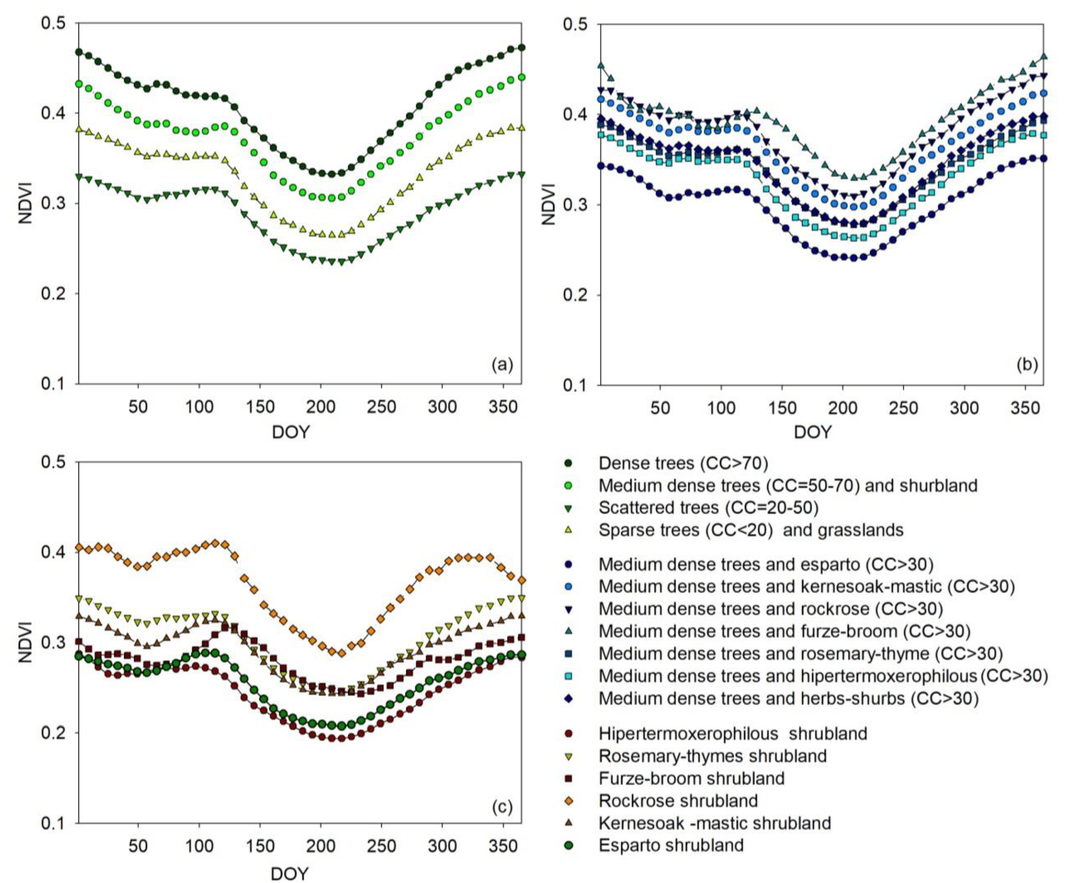
2.3.2. NDVI Annual Profile per Vegetation Type

Before correlating the ALS-based forest AGB assessment and MODIS-derived indices, we carried out a comparison among vegetation type profiles aimed at characterizing the influence of seasonal dynamics of the understory captured by satellite images on multilayer covers. This was performed mainly because grassland was excluded from ALS biomass estimation (see Section 2.2.1). Due to the relationship of the NDVI annual profile with green biomass [27,30], we generated the annual mean profile of an NDVI 8-day composite per vegetation type in the study area. Pixels of forest areas were aggregated into the main homogeneous vegetation formations at different percentages of canopy cover to describe their seasonal patterns. We classified the main vegetation in three cover types based on the SFM information: dense tree cover, mixed tree and shrub/herbs cover, and dense shrub/herbs cover. Each cover type was divided according to the vegetation species and canopy cover, which resulted in a set of 17 classes. To obtain the annual mean profile, the 8-day MODIS composite was layer-stacked to create a 46-band image for each year. We calculated the annual profile as the mean of the corresponding values of the three years considered (2015–2017).

2.3.3. MODIS Map: Spatial Predictive Model and Associated Uncertainty

The pixel values of the ALS benchmark map (250 m resolution) were considered as forest AGB synthetic data representative of the surface covered by the corresponding MODIS pixel. A systematic sample of pixels (39,647 pixels) was selected from the ALS benchmark map, increasing the distribution and sample size of the target variable (forest AGB). Covariate values were then extracted at each location from the covariate stack (Figure 1). The most explicative and low correlated predictors were selected through the VSURF package implemented in the R software [59] in combination with a low variance inflation factor (VIF, car package in R). Prior to the calculation of the VIF criterion, a GLM model was generated through the car package algorithm in R [71].

A machine learning algorithm was applied to model the relationship between the target variable (AGB obtained from the ALS benchmark map) and the covariates (selected MODIS derived indices and topographic factors). Due to the performance problems of RF with high dimensional data [72,73] and the need to conduct pixel-based uncertainty estimation, the extracted pixels of the ALS benchmark map were used to train a quantile regression forest (QRF). QRF is a generalization of RF used to estimate an accurate approximation of the full conditional distribution of the response variable. The QRF infers conditional quantiles to build predicted intervals interpreted as a surrogate of uncertainty associated with the response variable for each pixel value. The quantregForest package [74] was applied in the R software to perform predictive and uncertainty maps. Out-of-bag predictions were used to evaluate the quality of the conditional quantile approximations. We computed 2 maps at 250 m resolution: the predicted values of forest AGB based on MODIS-derived index and topographic factors, henceforth MODIS map, and their associated uncertainty. An independent validation of the predicted MODIS map was performed by testing a random sample of 3000 pixels from the ALS benchmark map. The linear correlation between tested and observed data showed the information values of the final MODIS map validation.

In order to analyze the relationship between estimated values of the final MODIS map and their associated uncertainty, a regression line was plotted to visually depict the forest AGB data and their corresponding relative uncertainty at 250 m pixel resolution.

According to [43], ignoring field-to-LiDAR uncertainty can lead to underestimation of estimator variance in a hierarchical modeling process. To address the analysis of the estimation accuracy in the up-scaling process, a generalized hierarchical model-based (ghmb) estimation was therefore performed based on the previous publication (ghmb, HMB package in R). To make the ghmb model computationally affordable, the dimension of the covariate space has been reduced based on the covariate’s importance measures depicted in the random forest analysis (randomForest package in R). Moreover, to reduce the number of input data (n = 39,647), a representative zone of the study area was selected (Figure 2). The results of the ghmb model are the estimated population mean of AGB and its variance as proxies of the estimation accuracy in the upscaling processes. For the same area, the AGB mean based on ALS map and MODIS map was also assessed to compare with the ghmb model results.

3. Results

3.1. ALS-Based Forest AGB Assessment

The VSURF procedure for variable selection has identified as the best combination of ALS-derived variables to predict forest AGB: mean height of total returns above 2 m (Hmean), 25th percentile of total returns above 2 m (Hp25), 50th percentile of total returns above 2 m (Hp50), tree canopy cover (TCC), and canopy cover of the low stratum (TCC_LS). The RF predictive model was calibrated and subsequently used to predict forest AGB at the field plots which were withheld from the model training subset at each cross-validation bootstrap. The RF model fitted with these variables showed a satisfactory performance in terms of variance explained and RMSE% (explained percentage variance: 69.09; median cross-validation RMSE%: 27.18).

The 25 m ALS map (Figure 2) showed remarkable spatial heterogeneity with a substantial increase in high elevation areas mainly distributed along the northwestern to southeastern axis of the study area. According to the 25 m ALS map prediction, the maximum values corresponded to the most densely forested areas mainly located in the middle and the northwest parts of the study area. By contrast, the minimum values were associated to shrubland areas. In the 25 m ALS map, the mean AGB value attained in forested areas was 25.44 t·ha⁻¹ and 21.7 t·ha⁻¹ standard deviation (sd). In tree cover areas (i.e., excluding pure shrubland area), the mean value of AGB was 37.64 t·ha⁻¹ (15.64 t·ha⁻¹ sd). Since the bilinear interpolation method used to compute the resampling from 25 to 250 m pixel resolution assigns the weighted average of nearest neighboring cells to the output cell value, the biomass mean value decreased at this moderate spatial resolution. Therefore, forest AGB at the 250 m pixel resolution showed a lower mean value and more homogeneous deviation at this coarser spatial resolution: 20.56 t·ha⁻¹ (18.57 t·ha⁻¹ sd). This resampled ALS biomass map was referred to as the forest ALS benchmark map.

3.2. From ALS Benchmark Map to MODIS Map

3.2.1. NDVI Annual Mean Profile per Vegetation Type

The signal of forest cover types was extracted from MODIS hypertemporal series of VIs which allowed to analyze valuable information about the vegetation phenology. The differences in seasonal patterns characterized various types of vegetation based on their NDVI annual profile. The comparison of the mean annual profile (8-day composite of the 2015–2017 time series) among the main vegetation formations allowed a discernment of the influence of vegetation different from tree and shrubland depending on the cover density level. The different forest cover types showed a dominant signal signature comparable to the tree canopy cover reflectance pattern (Figure 3a) even in combination with other shrub or grass vegetation types (Figure 3b,c). Most of the mean seasonal NDVI profiles of the vegetation types were characterized by a bimodal pattern with two maximum values in April–May (0.43 max in pine cover) and December–January (0.47 max in pine cover). The growing seasons started in March/April and September according to spring and autumn in the European Mediterranean basin. The tree-shrubland mixed cover (Figure 3b) presented the same profile pattern (i.e., shape) with slightly lower values than the tree cover (Figure 3a). The mean annual NDVI profile of pure shrubland of different vegetation formations revealed greater differences regarding the others forest cover types (Figure 3c). As stated before, the pure grassland cover was excluded for biomass prediction.

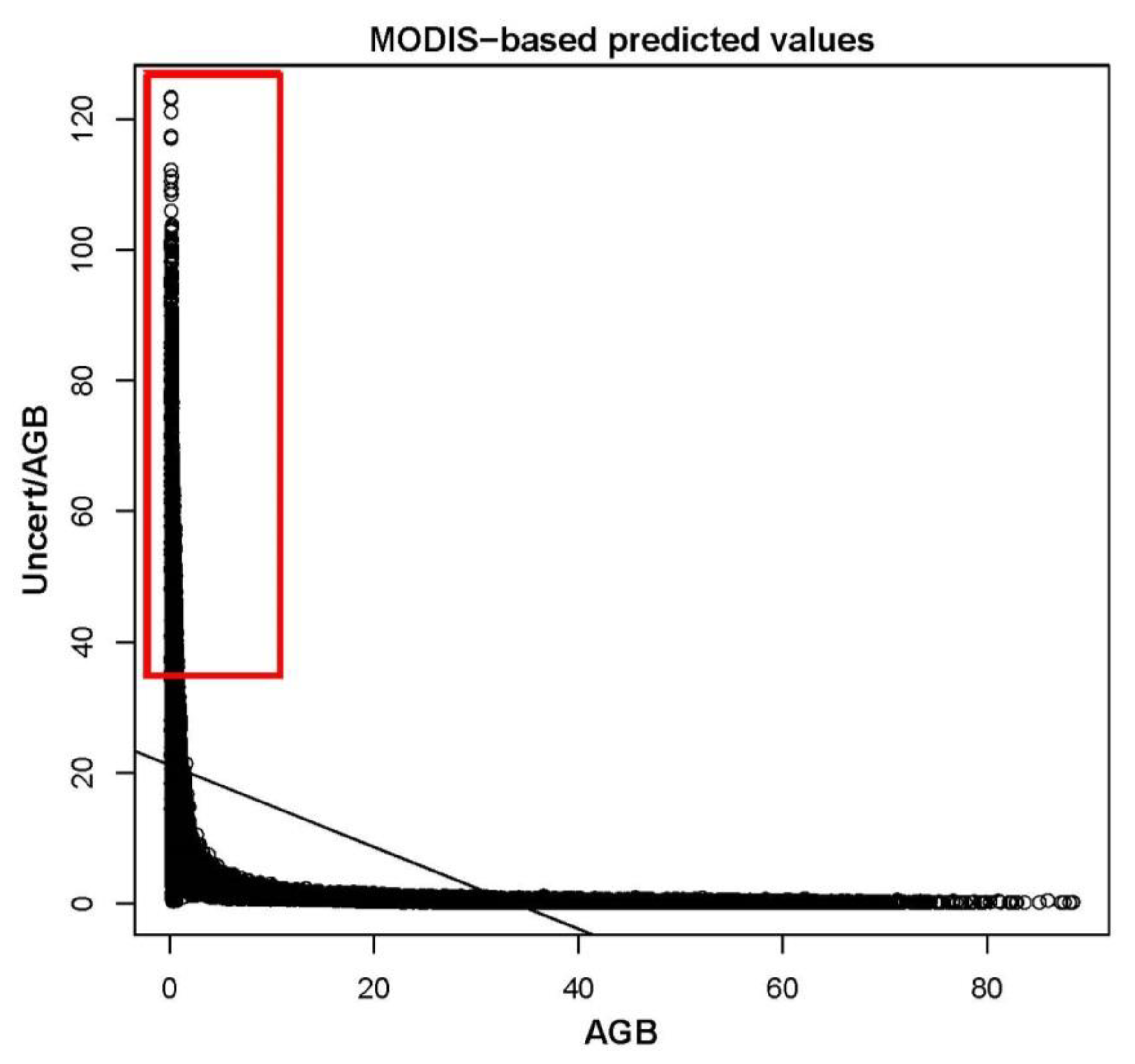
3.2.2. Model Fitting, Spatial Prediction, and Uncertainty Assessment

The previous VSURF selection of the initial set of 1060 covariates aimed to fit the predictive model from ALS benchmark map values decreased the dimension of the covariate space to 35 (

Table 4. Selected covariates in the fitted aboveground biomass predictive modeling of the airborne laser scanning (ALS) benchmark map.

Description	Selected	Covariates 1
8-day composite time series (2015–2017)	14/04/2016; 5&29/09/2016	NDVI,
	15/10/2016	MSR
8-day composite mean annual profile (2015–2017)	9/05; 21/08	NDVI,
16-day composite mean annual profile (2015–2017)	9/05; 13/08	EVI, NDW7
Mean value and standard deviation (2001–2016)	2 indices	NDVImean, NDVIsd
Maximum value (2015–2017)	6 indices	NDVI, MSR, DVI, RDVI, SAVI, MSAVI
Topographic variables	17 parameters	DEM, and 16 derived parameters included in Terrain Analyst functions (SAGA GIS software)

¹ Described in Table 3.

), after taking into account a low VIF criterion in order to minimize the statistical redundancy of the predictors. The dynamic predictive factors were associated to dates in April, early May, late August, September, and early October. NDVI was the main vegetation index at different time frames.

Then, two models were obtained through QFR which corresponded to conditional median for forest AGB (MODIS map) and conditional standard deviation, the latter as a surrogate of uncertainty. Based on the determination coefficient (R²) and the root-mean-square error (RMSE) as model information criteria, a substantial accuracy increase of the biomass estimates was observed in QRF models compared to GLM techniques previously generated to calculate the VIF. The latter showed an R² = 0.52 and RMSE = 12.9 t ha⁻¹ versus R² = 0.71 and RMSE = 9.97 t ha⁻¹ in the QRF model. The spatial interpolation of the two QRF models resulted into a 250 m spatial resolution map with two bands related to forest AGB estimate (MODIS map) and its associated uncertainty in each pixel (Figure 4).

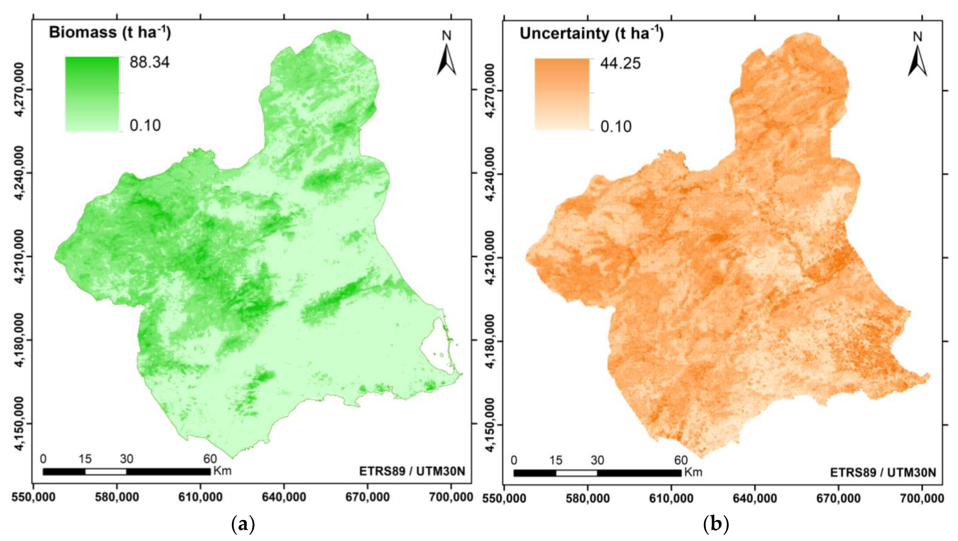
3.2.3. Final Predicted MODIS Map and Validation

Figure 4 depicts the spatial variability of the forest AGB MODIS map in the study area and its associated uncertainty. The biomass values ranged from 0.1 to 88.34 t ha⁻¹ and presented a very similar spatial distribution to the 25 m ALS map (see Figure 2). The highest AGB values also corresponded to tree cover in the central and northwest part of the study area, and the minimum ones were associated to shrubland covers in the southeast. The uncertainty values ranged from 0.1 to 44.25 t ha⁻¹, 11.34 t ha⁻¹, and 4.44 t ha⁻¹ as mean and sd values, respectively. The relationship between the forest AGB of MODIS map predicted values and their relative uncertainty associated the highest values of uncertainty with the lowest values (dots within the red box in Figure 5) and vice versa.

The resulting MODIS map also showed a predicted mean value very similar to the 25 m ALS map and slightly higher than the ALS benchmark map at 250 m: 24.91 t ha⁻¹ (17.16 t ha⁻¹ sd). Considering the associated uncertainty of MODIS-based predicted values, the results revealed a mean value of 18.77 t ha⁻¹ (13.31 t ha⁻¹ sd). The external, independent validation test attained a satisfactory fitting of the predictive model, since it presented a reasonable R² and similar RMSE (0.703 and 10.25 t ha⁻¹, respectively).

According to the AGB estimator for the global two-stage upscaling approach, the 35 selected covariates for AGB MODIS map modeling were reduced to 4 covariates based on the variable importance measures of the QRF model. These covariates were NDVI sd, 16-day NDVI composite of the 04/2016, 16-day EVI composite of the 08/2015 and DEM. The selected area for this analysis (Figure 2) covers an extent of 2773 km², and includes 72 field plots and a sample of 6474 pixels from the ALS benchmark map.

The ghmb model attained values of 41.63 t ha⁻¹ for the estimated AGB mean and 13.22 for the estimated variance with a 95% confidence interval of 34.51–48.76. Likewise, the AGB mean values were 34.72 t ha⁻¹ and 31.01 t ha⁻¹ for ALS and MODIS maps, respectively.

4. Discussion

4.1. Forest AGB Estimate from Local to National Scale

The assessment of forest aboveground biomass at the national extent and, subsequently, carbon stock is a future key challenge still unsolved in Spain with large implications related to climate change. The novelty of this study is to apply a two-stage upscaling process for AGB assessment over large extents using open data. Even though there is a time frequency inconsistence in ALS data in Spain, the provided methodology combines a sample of ALS data to bridge the scale gap between a sparse sample of field plots and satellite images.

The methodological framework presented herein provides a robust approach to map detailed, spatially continuous, and easy to update vegetation biomass from local to large scale. We demonstrated that forest attributes such as biomass can be modeled with relevant accuracy in large areas through optical remote sensing data as long as there is free availability of ALS data and NFI plots, such as in the case of Spain. This methodology has increasingly been employed [15] to estimate AGB across heterogeneous forested landscapes around the world [75]. Nevertheless, some authors such as that of [76] advised that LiDAR-based AGB assessment should be used with great care for further upscaling to satellite imagery, since they found lower uncertainties in NFI-calibrated biomass maps. The studies that considered the technique used in this study for feasible prediction of AGB refer to a reasonable density of training data to calibrate LiDAR data, short time lag data acquisition between NFI plots and LiDAR data, and a representative plot sample area related to LiDAR pixel resolution [38]. Once we addressed these considerations, the discrepancy between ALS biomass estimate and plot-level data was significantly reduced (Table 1) and, therefore, the error propagation, too. We obtained a satisfactory performance of the fitted model in terms of prediction of independent test data (explained percentage variance: 69.09; median cross-validation RMSE%: 27.18). As a general comparison, we contrasted our results with the review conducted by the authors of [77] over other forestry studies, which focused on estimating growing stock volume/biomass/carbon. All the considered studies in the review used field data, mostly from local inventories of NFIs, and contrasting sources of remotely sensed data. To facilitate the comparison of the results accuracy assessment, the RMSE% (defined as RMSE normalized by the mean observed values) was the measure most commonly used and attained a median RMSE% of 37%, with a standard deviation of ± 31.6% across these types of attributes. The studies that used only LiDAR-based feature variables (81 studies) revealed a median RMSE% of 31.3%, with a median reference set size of 124 plots (our study accounted for 242 plots). These studies confirmed that to obtain low RMSE%, large reference sets are necessary depending on the complexity and diversity of the forest. Therefore, our results of the AGB estimated based on the ALS model can be deemed as a promising result relative to these and national benchmarks [78].

Since the pixel values of the ALS benchmark map can be considered as forest AGB synthetic data, we integrated ALS pixel plots in order to increase the distribution and sample size of local data to model AGB at moderate resolution (250 m). As the authors of [41] claimed, this integration mitigates the cost of ground plot installation and offers spatially extensive and representative sampling of calibration and validation data to support the modeling of forest attributes, such as biomass canopy cover (in our study, more than 30,000 ALS plots and 3000 test data, respectively). However, the costs, limited revisited time and spatial continuity, logistics and data volumes involved in PNOA LiDAR data have fostered the combination of field NFI plot data and synthetic ALS dataset with MODIS imagery. As preliminary results, the extrapolation of AGB assessment from ALS to 250 m pixel resolution based on VIs and topographic variables (MODIS map) offered reasonably robust, accurate, and scalable results (R² 0.71 and RMSE 9.97 t ha⁻¹), with a satisfactory model fitting for the external, independent validation (similar R² and RMSE of 0.703 and 10.25 t ha⁻¹, respectively). Our MODIS model relative RMSE (48.47%) was consistent with other studies such as that of Reference [79], which revealed an RMSE% of 69% for aboveground tree biomass estimated by NFI ground plots and 250 m MODIS data. However, other studies, which a large amount of Landsat data, provided lower RMSE% at regional scale [80].

The main limitation of measure in our model was due to a discrepancy between the ALS estimation capacity and the surface reflectance signal captured by MODIS in grasslands. ALS presents measurement constraints related to its operational mode with discrete returns. It only returns a few (up to 4) points per laser shot and, therefore, represents a potential limitation for the measurement of short understory structure [81]. In this sense, canopy attribute measurement was correlated with the MODIS VIs reflectance signal, which also captures variability in understory structure related to composition and configuration of herbaceous species [82]. Our analysis of the NDVI annual profile characterizing the main types of vegetation in the Region of Murcia (Figure 3) showed slight differences in the shapes of seasonal patterns between stands of pure tree and mixed with grass or shrubland cover (Figure 3a–c), in which the pattern of the tree canopy cover was mainly predominant. This may be partially due to an understory scattered cover or an intermediate to dense pine canopy cover, where understory reflectance can be neglected.

In addition, since SNFI plots mainly encompass forest tree areas, biomass in pure shrub areas was estimated without plot-level validation. Therefore, and according to studies carried out by the authors of [83,84], high biomass uncertainties may be found in modeling herbs/shrub areas in the MODIS map generated in this study due to low ground cover or low vegetation height. Even though shrubland biomass estimation was less accurate, the model performance analysis revealed the convenience of including it, thus showing higher final model accuracy. This can be supported by the “edge effect” of the input data aggregation on upscaling [85] created in fragmented forest landscapes such as in the Region of Murcia, where tree canopy cover presented narrower and discontinuous spatial patches in comparison with the enlarged surface of shrubland. This is particularly relevant in forest biomass modeling in Mediterranean areas where fragmentation of forests is highly frequent due to strong human influence and management [86]. Moreover, in Mediterranean fire-prone landscapes, there is a current knowledge gap related to shrubland fuel load at the landscape scale and, therefore, lots of assumptions need to be taken in order to assess fire behavior at large scale [87]. In this sense, despite the acknowledged limitations, the shrubland AGB estimation carried out in this study represents a novel tool with relevant implications regarding fire regime modeling (and subsequently fire management, e.g., prescribed burning).

4.2. Environmental Drivers of Forest AGB Spatial Variability

Apart from the influence of dynamic type variables derived by optical remote sensing on AGB modeling, we also found a strong terrain variable influence. These factors derived from the DEM improved our forest AGB spatial estimate, though biomass changes cannot be detected from them, since topography is a static feature. The combination of both types of ecological drivers (static and dynamic) has overcome this limitation and allows us to monitor and easily update the biomass forest environmental changes.

Regarding the dynamic type variables, the previous covariates selection before modeling forest AGB at moderate spatial resolution showed that NDVI, combined with MSR and EVI, exerted a strong influence as environmental drivers among the estimated MODIS VIs. Because of the widely acknowledged close relationship between vegetation characteristics described by satellite data and biomass, remote sensing data are often used to calculate biomass estimates, showing a high correlation mainly with NDVI and describing similar insights as ours [88]. Moreover, our results revealed the importance of other covariates regarding different time dynamics which span from short to large time-scale, including seasonal mean dynamics.

The implementation of QRF to a large data set allows capturing complex hidden patterns between covariates and the response variable which are difficult to detect, or even difficult to interpret ecologically. In this sense, the results of our analysis showed quite consistent ecological interpretations. In the VIs time series, we found that the strongest correlation between forest AGB and VIs variables were associated with dates in April, September, and October 2016. This short-time response was related to the data acquisition during the 2016 ALS flight (from August to November), hence highlighting the importance of a short time lag in data acquisition between NFI plots and LiDAR data to minimize the outcome uncertainty [38]. In annual mean VIs profiles, we detected strong correlations with May and August dates coinciding with the end of the spring growing season and the start of the autumn growing season, respectively. While some covariates of short-time and annual mean scales were linked to different moments of the high photosynthetic activity in spring (beginning in March–April and reaching a maximum in May), the remaining covariates were related to the summer drought recovery, which is typical in the European Mediterranean region. Finally, long-term ecosystem functioning factors were represented by the mean annual and standard deviation of the NDVI time series as annual primary production and vegetation seasonality indicators [89].

In spite of the satisfactory model accuracy reported in this research, the fitted AGB model should be tested including other ground cover specific variables, such as forest canopy cover, and accounting for more species-specific equations to calculate AGB for Mediterranean shrubland. The latter may improve the assessment of forest AGB and its associated uncertainty, relevant in the two-stage upscaling methods due to the error propagation at all scales. In this sense, this can be checked when comparing the AGB mean assessed in each stage with the ghmb model results. The AGB mean of the ALS map for the specified testing area was within the 95% confidence interval of the ghmb model, whilst the MODIS map AGB mean was slightly out of the lower limit. Therefore, as [43] claimed, ignoring the uncertainty in the AGB benchmark map may lead to under-estimation of estimator variance in a hierarchical process. However, both methodologies—ghmb and random forest—are not totally comparable since they are based on different modeling approaches (linear regression vs. decision trees, respectively) and the number of covariates also differs. Despite this, an independent, external ground-based validation of the final MODIS map would be desirable, as it would allow the analysis of the accuracy and reduce the high uncertainty estimates which limit the understanding of the spatial variability of AGB.

5. Conclusions

The methodology proposed here has been shown to provide a cost-effective and easy to update model aimed at generating spatially extensive maps at management scales concordant with AGB complexity. This confirms our hypothesis regarding the correlation between ALS-based forest AGB and MODIS–derived VIs. In this study, we specifically leveraged the benefits of two complementary remote sensing technologies to map forest AGB over large areas and integrated ALS pixel plots as a means to increase the distribution and sample size of target data for modeling AGB as a function of VIs moderate resolution composites (MODIS).

The information necessary to perform the methodology tested in this study is available for the entire Spanish national territory and free to access. Even though there is a date inconsistency in ALS data in Spain with several years of time lag between two different areas owing to the time frequency of ALS flights each 6–7 years, enough networks of airborne ALS transect can be used to bridge the scale gap between field samples and satellite images. Due to the high temporal availability and moderate spatial resolution, MODIS imagery was shown to be feasible in forest AGB estimation for regional, even national, land use planning and management. The two-stage upscaling method for AGB assessment tested in this study can be applied over large areas, such as the whole country, to gain insights into national forest aboveground biomass, and subsequently into carbon stock, which remains a key challenge still unsolved in Spain.

References

1. Barredo, J.I.; Mauri, A.; Caudullo, G. Assessing Shifts of Mediterranean and Arid Climates Under RCP4.5 and RCP8.5 Climate Projections in Europe. Pure Appl. Geophys. 2018, 175, 3955–3971. [Google Scholar] [CrossRef] [Green Version]
2. Ometto, J.P.; Aguiar, A.P.; Assis, T.; Soler, L.; Valle, P.; Tejada, G.; Lapola, D.M.; Meir, P. Amazon forest biomass density maps: Tackling the uncertainty in carbon emission estimates. Clim Chang. 2014, 124, 545–560. [Google Scholar] [CrossRef]
3. Saatchi, S.; Houghton, R.A.; Dos Santos Alvalá, R.C.; Soares, J.V.; Yu, Y. Distribution of aboveground live biomass in the Amazon basin. Glob. Chang. Biol. 2007, 13, 816–837. [Google Scholar] [CrossRef] [Green Version]
4. Canadell, J.G.; Raupach, M.R. Managing forests for climate change mitigation. Science 2008, 320, 1456–1457. [Google Scholar] [CrossRef]
5. González-Jaramillo, V.; Fries, A.; Zeilinger, J.; Homeier, J.; Paladines-Benitez, J.; Bendix, J. Estimation of Above Ground Biomass in a Tropical Mountain Forest in Southern Ecuador Using Airborne LiDAR Data. Remote Sens. 2018, 10, 660. [Google Scholar] [CrossRef]
6. Navarro Cerrillo, R.M.; González Ferreiro, E.; García Gutiérrez, J.; Ceacero Ruiz, C.J.; Hernández Clemente, R. Impact of plot size and model selection on forest biomass estimation using airborne LiDAR: A case study of pine plantations in southern Spain. J. For. Sci. 2017, 63, 88–97. [Google Scholar] [CrossRef] [Green Version]
7. Næsset, E.; Gobakken, T. Estimation of above-and below-ground biomass across regions of the boreal forest zone using airborne laser. Remote Sens. Environ. 2008, 112, 3079–3090. [Google Scholar] [CrossRef]
8. White, J.C.; Coops, N.C.; Wulder, M.A.; Vastaranta, M.; Hilker, T.; Tompalski, P. Remote sensing technologies for enhancing forest inventories: A review. Can. J. Remote Sens. 2016, 42, 619–641. [Google Scholar] [CrossRef]
9. Valbuena, R.; De Blas, A.; Martín Fernández, S.; Maltamo, M.; Nabuurs, G.J.; Manzanera, J.A. Within-Species Benefits of Back-projecting Laser Scanner and Multispectral Sensors in Monospecific P. sylvestris Forests. Eur. J. Remote Sens. 2013, 46, 491–509. [Google Scholar] [CrossRef]
10. Bottalico, F.; Chirici, G.; Giannini, R.; Mele, S.; Mura, M.; Puxeddu, M.; McRoberts, R.E.; Valbuena, R.; Travaglini, D. Modeling Mediterranean Forest Structure Using Airborne Laser Scanning Data. Int. J. Appl. Earth Obs. 2017, 57, 145–153. [Google Scholar] [CrossRef]
11. Kauranne, T.; Joshi, A.; Gautam, B.; Manandhar, U.; Nepal, S.; Peuhkurinen, J.; Hämäläinen, J.; Junttila, V.; Gunia, K.; Latva-Käyrä, P.; et al. LiDAR-Assisted Multi-Source Program (LAMP) for Measuring Above Ground Biomass and Forest Carbon. Remote Sens. 2017, 9, 154. [Google Scholar] [CrossRef]
12. Molina, P.X.; Asner, G.P.; Farjas Abadía, M.; Ojeda Manrique, J.C.; Sánchez Diez, L.A.; Valencia, R. Spatially-Explicit Testing of a General Aboveground Carbon Density Estimation Model in a Western Amazonian Forest Using Airborne LiDAR. Remote Sens. 2016, 8, 9. [Google Scholar] [CrossRef]
13. Maltamo, M.; Packalén, P.; Suvanto, A.; Korhonen, K.T.; Mehtätalo, L.; Hyvönen, P. Combining ALS and NFI training data for forest management planning: A case study in Kuortane, Western Finland. Eur. J. For. Res. 2009, 128, 305. [Google Scholar] [CrossRef]
14. Nelson, R.; Gobakken, T.; Næsset, E.; Gregoire, T.; Ståhl, G.; Holm, S.; Flewelling, J. Lidar sampling—Using an airborne profiler to estimate forest biomass in Hedmark County, Norway. Remote Sens. Environ. 2012, 123, 563–578. [Google Scholar] [CrossRef]
15. Fassnacht, F.E.; Latifi, H.; Hartig, F. Using synthetic data to evaluate the benefits of large field plots for forest biomass estimation with LiDAR. Remote Sens. Environ. 2018, 213, 115–128. [Google Scholar] [CrossRef]
16. Hudak, A.T.; Strand, E.K.; Vierling, L.A.; Byrne, J.C.; Eitel, J.U.H.; Martinuzzi, S.; Falkowski, M.J. Quantifying aboveground forest carbon pools and fluxes from repeat LiDAR surveys. Remote Sens. Environ. 2012, 123, 25–40. [Google Scholar] [CrossRef]
17. Cash, D.W.; Moser, S.C. Linking global and local scales: Designing dynamic assessment and management processes. Glob. Environ. Chang. 2000, 10, 109–120. [Google Scholar] [CrossRef]
18. Lu, D. The potential and challenge of remote sensing-based biomass estimation. Int. J. Remote Sens. 2006, 27, 1297–1328. [Google Scholar] [CrossRef]
19. Xiao, J.; Moody, A. Photosynthetic activity of US biomes: Responses to the spatial variability and seasonality of precipitation and temperature. Glob Chang Biol. 2004, 10, 437–451. [Google Scholar] [CrossRef]
20. Blackard, J.A.; Finco, M.V.; Helmer, E.H.; Holden, G.R.; Hoppus, M.L.; Jacobs, D.M.; Lister, A.J.; Moisen, G.G.; Nelson, M.D.; Riemann, R.; et al. Mapping U.S. forest biomass using nationwide forest inventory data and moderate resolution information. Remote Sens. Environ. 2008, 112, 1658–1677. [Google Scholar] [CrossRef]
21. Chi, H.; Sun, G.; Huang, J.; Guo, Z.; Ni, W.; Fu, A. National Forest Aboveground Biomass Mapping from ICESat/GLAS Data and MODIS Imagery in China. Remote Sens. 2015, 7, 5534–5564. [Google Scholar] [CrossRef] [Green Version]
22. Jin, Y.; Yang, X.; Qiu, J.; Li, J.; Gao, T.; Wu, Q.; Zhao, F.; Ma, H.; Yuand, H.; Xu, B. Remote sensing-based biomass estimation and its spatio-temporal variations in temperate grassland, Northern China. Remote Sens. 2014, 6, 1496–1513. [Google Scholar] [CrossRef]
23. Didan, K. MOD13Q1 MODIS/Terra Vegetation Indexes 16-Day L3 Global 250 m SIN Grid V006 [Data Set]; NASA EOSDIS LP DAAC: Sioux Falls, SD, USA, 2015. [CrossRef]
24. Reed, B.C.; Schwartz, M.D.; Xiangming, X. Remote sensing phenology: Status and the way forward. In Phenology of Ecosystem Processes; Noormets, A., Ed.; Springer: New York, NY, USA, 2009; pp. 231–246. ISBN 978-1-4419-0026-5. [Google Scholar]
25. Le, L.; Guo, Q.; Tao, S.; Kelly, M.; Xu, G. Lidar with multi-temporal MODIS provide a means to upscale predictions of forest biomass. ISPRS J. Photogramm. Remote Sens. 2015, 102, 198–208. [Google Scholar] [CrossRef]
26. Tucker, C.J. Red and photographic infrared linear combinations for monitoring vegetation. Remote Sens. Environ. 1979, 8, 127–150. [Google Scholar] [CrossRef] [Green Version]
27. Paruelo, J.M.; Epstein, H.E.; Lauenroth, W.K.; Burke, I.C. ANPP estimates from NDVI for the central grassland region of the United States. Ecology 1997, 78, 953–958. [Google Scholar] [CrossRef]
28. Piao, S.; Friedlingstein, P.; Ciais, P.; de Noblet-Ducoudré, N.; Labat, D.; Zaehle, S. Changes in climate and land use have a larger direct impact than rising CO2 on global river runoff trends. Proc. Natl. Acad. Sci. USA 2007, 4, 15242–15247. [Google Scholar] [CrossRef] [PubMed]
29. Yan, F.; Wu, B.; Wang, Y. Estimating spatiotemporal patterns of aboveground biomass using Landsat TM and MODIS images in the Mu Us Sandy Land, China. Agric. For. Meteorol. 2015, 200, 119–128. [Google Scholar] [CrossRef]
30. Alcaraz-Segura, D.; Cabello, J.; Paruelo, J.; Delibes, M. Use of Descriptors of Ecosystem Functioning for Monitoring a National Park Network: A Remote Sensing Approach. Environ. Manag. 2009, 43, 38–48. [Google Scholar] [CrossRef]
31. Tenkabail, P.S.; Smith, R.B.; Pauw, E.D. Hyperspectral vegetation indices and their relationships with agricultural crop characteristics. Remote Sens. Environ. 2000, 75, 158–182. [Google Scholar] [CrossRef]
32. Liu, Q.; Huete, A. A feedback based modification of the NDVI to minimize canopy background and atmospheric noise. IEEE Trans. Geosci. Remote Sens. 1995, 33, 457–465. [Google Scholar] [CrossRef]
33. Huete, A.R. A soil adjusted vegetation index (SAVI). Remote Sens. Environ. 1988, 25, 295–309. [Google Scholar] [CrossRef]
34. Mutanga, O.; Skidmore, A.K. Narrow band vegetation indices solve the saturation problem in biomass estimation. Int. J. Remote Sens. 2004, 25, 3999–4014. [Google Scholar] [CrossRef]
35. Rougean, J.L.; Breon, F.M. Estimating PAR absorbed by vegetation from bidirectional reflectance measurements. Remote Sens. Environ. 1995, 51, 375–384. [Google Scholar] [CrossRef]
36. Jordan, C.F. Derivation of leaf area index from quality of light on the forest floor. Ecology 1969, 50, 663–666. [Google Scholar] [CrossRef]
37. Chen, J. Evaluation of vegetation indexes and modified simple ratio for boreal applications. Can. J. Remote Sens. 1996, 22, 229–242. [Google Scholar] [CrossRef]
38. Matasci, G.; Hermosilla, T.; Wulder, M.A.; White, J.C.; Coops, N.C.; Hobart, G.W.; Zald, H.S. Large-area mapping of Canadian boreal forest cover, height, biomass and other structural attributes using Landsat composites and lidar plots. Remote Sens. Environ. 2018, 209, 90–106. [Google Scholar] [CrossRef]
39. Moore, I.D.; Grayson, R.B.; Ladson, A.R. Digital terrain modelling: A review of hydrological, geomorphological, and biological applications. Hydrol. Process. 1991, 5, 3–30. [Google Scholar] [CrossRef]
40. Mendoza Ponce, A.; Corona Núñez, R.; Kraxnera, F.; Leduca, S.; Patrizioa, P. Identifying effects of land use cover changes and climate change on terrestrial ecosystems and carbon stocks in Mexico. Glob. Environ. Chang. 2018, 53, 12–23. [Google Scholar] [CrossRef]
41. Wulder, M.A.; White, J.C.; Nelson, R.F.; Næsset, E.; Ørka, H.O.; Coops, N.C.; Hilker, T.; Bater, C.B.; Gobakken, T. Lidar sampling for large-area forest characterization: A review. Remote Sens. Environ. 2012, 121, 196–209. [Google Scholar] [CrossRef] [Green Version]
42. Navarro, J.A.; Algeet, N.; Fernández-Landa, A.; Esteban, J.; Rodríguez-Noriega, P.; Guillén-Climent, M.L. Integration of UAV, Sentinel-1, and Sentinel-2 Data for Mangrove Plantation Aboveground Biomass Monitoring in Senegal. Remote Sens. 2019, 11, 77. [Google Scholar] [CrossRef]
43. Saarela, S.; Holm, S.; Grafström, A.; Schnell, S.; Næsset, E.; Gregoire, T.G.; Nelson, R.F.; Ståhl, G. Hierarchical model-based inference for forest inventory utilizing three sources of information. Ann. For. Sci. 2016, 73, 895–910. [Google Scholar] [CrossRef] [Green Version]
44. Papadakis, J. Climates of the World and their Agricultural Potentialities; J. Papadakis: Buenos Aires, Argentina, 1966; ISBN 19670701017. [Google Scholar]
45. Ministerio de Agricultura, Alimentación y Medio Ambiente (MAGRAMA). Cuarto Inventario Forestal Nacional. Región de Murcia; Organismo Autónomo Parques Nacionales: Madrid, Spain, 2012; 44p, ISBN 978-84-8014-820-7. [Google Scholar]
46. Murgaš, V.; Sačkov, I.; Sedliak, M.; Tunák, D.; Chudý, F. Assessing horizontal accuracy of inventory plots in forests with different mix of tree species composition and development stage. J. For. Sci. 2018, 64, 478–485. [Google Scholar] [CrossRef]
47. Mauro, F.; Valbuena, R.; Manzanera, J.A.; García-Abril, A. Influence of Global Navigation Satellite System errors in positioning inventory plots for tree-height distribution studies. Can. J. For. Res. 2011, 41, 11–23. [Google Scholar] [CrossRef]
48. Fernández-Landa, A.; Fernández-Moya, J.; Tomé, J.L.; Algeet-Abarquero, N.; Guillén-Climent, M.L.; Vallejo, R.; Marchamalo, M. High resolution forest inventory of pure and mixed stands at regional level combining National Forest Inventory field plots, Landsat, and low density lidar. Int. J. of Rem. Sen. 2018, 39, 4830–4844. [Google Scholar] [CrossRef]
49. Magnussen, S.; Boudewyn, P. Derivations of stand heights from airborne laser scanner data with canopy-based quantile estimators. Can. J. For. Res. 1998, 28, 1016–1031. [Google Scholar] [CrossRef]
50. Montero, G.; Ruiz-Peinado, R.; Muñoz, M. Producción de Biomasa y fijación de CO2 por los Bosques Españoles; INIA (MEC): Madrid, Spain, 2005; ISBN 9788474985122. [Google Scholar]
51. Montero, G.; Pasalodos-Tato, M.; López-Senespleda, E.; Onrubia, R.; Madrigal, G. Ecuaciones para la Estimación de la Biomasa en Matorrales y arbustedos mediterráneos. 6º Congreso Forestal Español; Sociedad Española de Ciencias Forestales: Vitoria-Gasteiz, Spain, 2013. [Google Scholar]
52. Domingo, D.; Alonso, R.; Lamelas, M.T.; Montealegre, A.L.; Rodríguez, F.; de la Riva, J. Temporal Transferability of Pine Forest Attributes Modeling Using Low-Density Airborne Laser Scanning Data. Remote Sens. 2019, 11, 261. [Google Scholar] [CrossRef]
53. McGaughey, R.J.; Carson, W.W. Fusing LIDAR data, photographs, and other data using 2D and 3D visualization techniques. Proc. Terrain Data Appl. Vis.—Mak. Connect. 2003, 28–30. Available online: https://bit.ly/2UaNGlm (accessed on 18 November 2018).
54. Næsset, E. Predicting Forest Stand Characteristics with Airborne Scanning Laser Using a Practical Two-Stage Procedure and Field Data. Remote Sens. Environ. 2002, 80, 88–99. [Google Scholar] [CrossRef]
55. Pike, R.J.; Wilson, S.E. Elevation-Relief Ratio, Hypsometric Integral, and Geomorphic Area-Altitude Analysis. GSA Bull. 1971, 82, 1079–1084. [Google Scholar] [CrossRef]
56. Parker, G.G.; Russ, M.E. The Canopy Surface and Stand Development: Assessing Forest Canopy Structure and Complexity with near-Surface Altimetry. For. Ecol. Manag. 2004, 189, 307–315. [Google Scholar] [CrossRef]
57. Breiman, L. Random forests. Mach. Learn. 2001, 45, 5–32. [Google Scholar] [CrossRef]
58. Liaw, A.; Wiener, M. Classification and regression by random forest. R News 2002, 2, 18–22. [Google Scholar]
59. Genuer, R.; Poggi, J.M.; Tuleau-Malot, C.; Genuer, M.R. Package ‘vsurf’. Pattern Recognit. Lett. 2015, 14, 2225–2236. [Google Scholar]
60. Evans, J.S.; Murphy, M.A. rfUtilities. R Package Version 2.1-3. 2018. Available online: https://cran.r-project.org/web/packages/rfUtilities/index.html (accessed on 18 November 2018).
61. R Development Core Team. R: A Language and Environment for Statistical Computing; R Development Core Team: Vienna, Austria, 2014. [Google Scholar]
62. Hijmans, R.J. Package ‘raster’. R Package Version 2.8-4. 2018. Available online: https://cran.r-project.org/web/packages/raster/index.html (accessed on 20 November 2018).
63. Vermote, E. MOD09Q1 MODIS/Terra Surface Reflectance 8-Day L3 Global 250 m SIN Grid V006 [Data Set]; NASA EOSDIS LP DAAC: Sioux Falls, SD, USA, 2015.
64. NASA Land Processes Distributed Active Archive Center. Available online: https://lpdaac.usgs.gov/ (accessed on 25 October 2018).
65. Gao McNairn, H.; Protz, R. Mapping corn residue cover on agricultural fields in Oxford County, Ontario, using Thematic Mapper. Can. J. Remote Sens. 1993, 19, 152–159. [Google Scholar] [CrossRef]
66. Qi, J.; Chehbouni, A.; Huete, A.R.; Kerr, Y.H.; Sorooshian, S. A modified soil adjusted vegetation index. Remote Sens. Environ. 1994, 48, 119–126. [Google Scholar] [CrossRef]
67. Pettorelli, N.; Vik, J.O.; Mysterud, A.; Gaillard, J.M.; Tucker, C.J.; Stenseth, N.C. Using the satellite-derived NDVI to assess ecological responses to environmental change. Trends Ecol. Evol. 2005, 20, 503–510. [Google Scholar] [CrossRef] [PubMed]
68. Holben, B.N. Characteristics of maximum value composite images for temporal AVHRR data. Int. J. Remote Sens. 1986, 7, 1417–1437. [Google Scholar] [CrossRef]
69. Wilson, D.S.; Jamieson, S.S.; Barrett, P.J.; Leitchenkov, G.; Gohl, K.; Larter, R.D. Antarctic topography at the Eocene–Oligocene boundary. Palaeogeogr. Palaeoclimatol. Palaeoecol. 2012, 335–336, 24–34. [Google Scholar] [CrossRef]
70. Conrad, O.; Bechtel, B.; Bock, M.; Dietrich, H.; Fischer, E.; Gerlitz, L.; Wehberg, J.; Wichmann, V.; Böhner, J. System for Automated Geoscientific Analyses (SAGA) v. 2.1.4. Geosci. Model Dev. 2015, 8, 1991–2007. [Google Scholar] [CrossRef]
71. Fox, J. Applied Regression Analysis and Generalized Linear Models, 3rd ed.; SAGE: Thousand Oaks, CA, USA, 2016; ISBN 978-1-4522-0566. [Google Scholar]
72. Do, T.N.; Lenca, P.; Lallich, S.; Pham, N.K. Classifying very-high-dimensional data with random forests of oblique decision trees. In Advances in Knowledge Discovery and Management; Guillet, F., Pinaud, B., Venturini, G., Zighed, D.A., Eds.; Springer: Berlin/Heidelberg, Germany, 2010; pp. 39–55. ISBN 978-3-642-00580-0. [Google Scholar]
73. Xu, B.; Huang, J.Z.; Williams, G.; Wang, Q.; Ye, Y. Classifying very high-dimensional data with random forests built from small subspaces. Int. J. Data Wareh. Min. 2012, 8, 44–63. [Google Scholar] [CrossRef]
74. Meinshausen, N. quantregForest: Quantile Regression Forests. R Package version 1.3-7, 2017. Available online: https://CRAN.R-project.org/package=quantregForest (accessed on 22 November 2018).
75. Flilnt, R.; Gregory, P.A.; Baldwine, J.A.; Mascaroc, J.; Bufild, L.K.K.; Knappb, D.E. Estimating aboveground carbon density across forest landscapes of Hawaii: Combining FIA plot-derived estimates and airborne LiDAR. For. Ecol. Manag. 2018, 424, 323–337. [Google Scholar] [CrossRef]
76. Urbazaev, M.; Thiel, C.; Cremer, F.; Dubayah, R.; Migliavacca, M.; Reichstein, M.; Schmullius, C. Estimation of forest aboveground biomass and uncertainties by integration of field measurements, airborne lidar, and sar and optical satellite data in México. Carbon Balance Manag. 2018, 13, 5. [Google Scholar] [CrossRef]
77. Chirici, G.; Mura, M.; Mcinerney, D.; Py, N.; Tomppo, E.O.; Waser, L.T.; Travaglini, D.; Mcroberts, R.E. A meta-analysis and review of the literature on the k-Nearest Neighbors technique for forestry applications that use remotely sensed data. Remote Sens. Environ. 2016, 176, 282–294. [Google Scholar] [CrossRef]
78. Domingo, D.; Lamelas, M.T.; Montealegre, A.L.; García-Martín, A.; De la Riva, J. Estimation of Total Biomass in Aleppo Pine Forest Stands Applying Parametric and Nonparametric Methods to Low-Density Airborne Laser Scanning Data. Forests 2018, 9, 158. [Google Scholar] [CrossRef]
79. Beaudoin, A.; Bernier, P.Y.; Guindon, L.; Villemaire, P.; Guo, X.J.; Stinson, G.; Magnussen, S.; Hall, R.J. Mapping attributes of Canada’s forests at moderate resolution through kNN and MODIS imagery. Can. J. For. Res. 2014, 44, 521–532. [Google Scholar] [CrossRef]
80. Nguyen, T.H.; Jones, S.; Soto-Berelov, M.; Haywood, A.; Hislop, S. A Comparison of Imputation Approaches for Estimating Forest Biomass Using Landsat Time-Series and Inventory Data. Remote Sens. 2018, 10, 1825. [Google Scholar] [CrossRef]
81. Hancock, S. Measurement of fine-spatial-resolution 3D vegetation structure with airborne waveform lidar: Calibration and validation with voxelised terrestrial lidar. Remote Sens. Environ. 2016, 188, 37–50. [Google Scholar] [CrossRef]
82. Ozdemir, I. Linear transformation to minimize the effects of variability in understory to estimate percent tree canopy cover using RapidEye data. GIsci. Remote Sens. 2014, 51, 288–300. [Google Scholar] [CrossRef]
83. Li, A.; Dhakal, S.; Glenn, N.F.; Spaete, L.P.; Shinneman, D.J.; Pilliod, D.S.; Arkle, R.S.; McIlroy, S.K. Lidar aboveground vegetation biomass estimates in shrublands: Prediction, uncertainties and application to coarser scales. Remote Sens. 2017, 9, 903. [Google Scholar] [CrossRef]
84. Glenn, N.F.; Neuenschwander, A.; Vierling, A.A.; Spaete, L.P.; Li, A.; Shinneman, D.; Pilliod, D.S.; Arkle, R.; McIlroy, S. Landsat 8 and ICESat-2: Performance and potential synergies for quantifying dryland ecosystem vegetation cover and biomass. Remote Sens. Environ. 2016, 185, 233–242. [Google Scholar] [CrossRef]
85. He, S.H.; Ventura, J.S.; Mladenoff, J.D. Effects of spatial aggregation approaches on classified satellite imagery. Int. J. Geogr. Inf. Syst. 2002, 16, 93–109. [Google Scholar] [CrossRef] [Green Version]
86. Doblas-Miranda, E.; Martínez-Vilalta, J.; Lloret, F.; Álvarez, A.; Ávila, A.; Bonet, F.J.; Brotons, L.; Castro, J.; Curiel Yuste, J.; Díaz, M.; et al. Reassessing global change research priorities in Mediterranean terrestrial ecosystems: How far have we come and where do we go from here? Glob. Ecol. Biogeogr. 2014, 24, 25–43. [Google Scholar] [CrossRef]
87. Duane, A.; Aquilué, N.; Gil-Tena, A.; Brotons, L. Integrating fire spread patterns in fire modelling at landscape scale. Environ. Model. Softw. 2016, 86, 219–231. [Google Scholar] [CrossRef]
88. Mura, M.; Bottalico, F.; Giannetti, F.; Bertani, R.; Giannini, R.; Mancini, M.; Orlandini, S.; Travaglini, D.; Chirici, G. Exploiting the capabilities of the Sentinel-2 multi spectral instrument for predicting growing stock volume in forest ecosystems. Int. J. Appl. Earth Obs. Geoinf. 2018, 66, 126–134. [Google Scholar] [CrossRef]
89. Huete, A.; Didan, K.; Miura, T.; Rodriguez, E.P.; Gao, X.; Ferreira, L.G. Overview of the radiometric and biophysical performance of the MODIS vegetation indexes. Remote Sens. Environ. 2002, 83, 195–213. [Google Scholar] [CrossRef]
Figure 1. Methodological scheme of the target and predictor variables extraction for modeling the final moderate-resolution aboveground biomass.
Remotesensing 11 00795 g001
Figure 2. 25 m airborne laser scanning (ALS) map of aboveground biomass estimation (t ha−1) in the Region of Murcia (Spain), which was calibrated with plot-level ground-based measures (14.1 m radius plots were represented as black dots and were based on the SNFI). The inner rectangle depicts the selected testing area to estimate the global estimator variance through ghmb.
Remotesensing 11 00795 g002
Figure 3. (ac): NDVI annual mean profile of the 8-day MODIS composite of the 2015–2017 time series per main vegetation types and percentage of canopy cover (CC) based on Spanish forest map (SFM) information. DOY: day of the year.
Remotesensing 11 00795 g003
Figure 4. Maps of (a) MODIS-based predicted values of aboveground forest biomass (t ha−1) in the Region of Murcia (Spain) and (b) associated uncertainty estimated through the quantile regression forest (QRF) method. The display has been stretched by means of a cumulative pixel count cut method (default range 2–98%).
Remotesensing 11 00795 g004
Figure 5. Contrast between the predicted values of the MODIS-based aboveground biomass (AGB) and their associated relative uncertainty (uncertainty/AGB).
Remotesensing 11 00795 g005