Classification of North Africa for Use as an Extended Pseudo Invariant Calibration Sites (EPICS) for Radiometric Calibration and Stability Monitoring of Optical Satellite Sensors

Abstract

Pseudo invariant calibration sites (PICS) have been extensively used for the radiometric calibration and temporal stability monitoring of optical satellite sensors. Due to limited knowledge about the radiometric stability of North Africa, only a limited number of sites in the region are used for this purpose. This work presents an automated approach to classify North Africa for its potential use as an extended PICS (EPICS) covering vast portions of the continent. An unsupervised classification algorithm identified 19 “clusters” representing distinct land surface types was used; three clusters were identified with spatial uncertainties within approximately 5% in the shorter wavelength bands and 3% in the longer wavelength bands. A key advantage of the cluster approach is that large numbers of pixels are aggregated into contiguous homogeneous regions sufficiently distributed across the continent to allow multiple imaging opportunities per day, as opposed to imaging a typical PICS once during the sensor’s revisit period. This potential increase in temporal resolution could result in increased sensitivity for the quicker identification of changes in sensor response.

1. Introduction

For over 45 years, data from Earth observing satellite sensors have been used to increase the understanding of long-term global change. Thus, the quality of data produced by previous and currently operational sensors is a primary concern, as it critically depends on accurate radiometric calibration for each sensor. Accurate radiometric calibration also allows meaningful comparisons of data acquired by different sensors to be combined into a continuous record [1]. Radiometric calibration needs to be performed both before launch (to establish an initial operating state) and at regular intervals after launch (to account for degradations in response due to launch stresses, aging and effects relating to conditions in near-Earth orbit). Sensors often include onboard calibrators (e.g., solar diffuser panels, lamps, thermal blackbody radiators) intended to provide data for radiometric calibration and long-term stability monitoring.

Since an onboard calibrator experiences conditions similar to the sensor, its data will likely show similar degradation in radiometric response. Onboard calibrator systems can increase the design, building, and operating costs of a sensor and are thus not included in all satellites, especially those designed with shortened operating lifetimes. Alternatively, image data from locations on the earth’s surface exhibiting minimal temporal change and other desirable properties have been identified and are increasingly used as a calibration data source; these sites are known as pseudo-invariant calibration sites (PICS) [2]. Any changes in a sensor’s radiometric response can then be attributed to changes in the sensor itself, rather than to changes at the PICS. Teillet et al. [3,4] provided a comprehensive list of PICS suitable for post launch radiometric calibration, sensor cross calibration, and long-term stability monitoring. Some of these sites have since been endorsed by the Committee on Earth Observing Sensors (CEOS).

Primarily, PICS are used for three purposes: long term trending to assess sensor radiometric stability, cross calibration of sensors, and absolute radiometric calibration. PICS are most widely used to monitor the post launch degradation of sensors [5,6,7,8,9,10,11]. Using data from the CEOS-recommended standard PICS, Chander et al. [5] investigated on-orbit stability of the Terra MODIS and ETM+ sensors, and found that both sensors’ measured TOA reflectances changed less than 0.4% per year. Several researchers have used PICS for cross calibration of sensors as well [12,13,14,15,16]. Li et al. [17] used PICS to cross calibrate the recently launched Sentinel-2A MSI to the OLI and estimated agreement between the corresponding bands to approximately 1% or better. Furthermore, absolute calibration predicts the TOA reflectance, or radiance, observed by the sensor at any given geometry [18,19,20,21,22]. A recent absolute radiometric calibration model develop by Bouvet can accurately simulate the VNIR band TOA reflectance of Libya 4 to within 1% of observed values [23].

1.1. Historical Approach for Identifying Candidate PICS

Previous work in the search for suitable PICS has been limited to a few regions within the Sahara Desert, often based on visual inspection of cloud-free image data to identify candidate spatially homogeneous areas. Using Meteosat-4 data, Cosnefroy et al. [24] selected 20 desert sites of size 100 × 100 km in North Africa and Saudi Arabia with estimated spatial uncertainties of 3% or less and temporal uncertainties between approximately 1% and 2%. They determined, for some of the selected sites and over short time intervals, that the most spatially stable sites also tended to be the most temporally stable sites. Helder et al. [2] developed an automated technique to locate temporally and spatially optimal stable regions. Using Landsat 5 TM image data, they found six individual sites in the Sahara and Middle East exhibiting spatial and temporal uncertainties on the order of 2% in the VNIR region and 2–3% in the SWIR region.

1.2. Limitations of Using Traditional PICS

Imaging of individual PICS such as Libya 4 is limited by a sensor’s orbital path, field of view (FOV), and occurrence of cloud cover, which results in an observation frequency far lower than that potentially offered by the sensor’s revisit cycle and assuming cloud-free conditions. As a result, more time is required to build a time series dataset with sufficient observations to allow reasonable radiometric analyses with adequate sensitivity. An additional limitation of PICS used for cross-calibration is a lack of surface hyperspectral knowledge at most of the sites.

This limitation imposed by traditional PICS can be addressed by extending PICS to a larger region than it used to be. Ruchira [25] performed an initial study on searching worldwide PICS and she showed that majority region of North Africa are stable to some degree. These stable surfaces are of different intensity level so it is necessary to identify the stable regions having similar spectral profiles in order to expand them for developing extended PICS. These spectrally similar regions of North Africa can be found by developing a classification map of North Africa.

1.3. Previous Classification of North Africa

Loveland et al. [26] applied an unsupervised classification algorithm to Advanced Very High-Resolution Radiometer (AVHRR) image data to develop a land cover characteristics database for the conterminous US. Using a supervised algorithm, Hansen et al. [27] developed the first global land cover classification using 1 km spatial resolution AVHRR data; their training dataset was previously generated from higher spatial resolution data. Interestingly, both classification methods identified a generic “barren” class, which was defined as land cover having less than 10% vegetation throughout the year; this class included all soils, rocks, and sands. A similar global land cover product was also generated for Terra MODIS using a supervised classification algorithm, with training datasets derived from higher resolution image data and ground-based surface reflectance measurements when available [28]. It also identified a generic “barren” class across North Africa.

To the present time, the “barren” classification is still used to group all soil, sand, and rock land cover types into a single land cover type, as most applications using land cover data do not require such a fine distinction. However, this “barren” land cover also includes spatially and temporally stable ground cover types that are highly desirable with respect to PICS-based radiometric calibration. Consequently, the “barren” land cover type identified in North Africa should be resolved into subclasses, which would allow the evaluation of their radiometric intensity and stability for potential use in calibration across wider portions of a sensor’s dynamic range.

1.4. Current Approach for Extending PICS

Spectral properties of North Africa have been only studied superficially due to lack of its significance to the scientific community. As its majority of regions are stable, it should be studied more rigorously in order to utilize these regions for radiometric calibration of optical satellite sensors. So, the primary concern of this work is to characterize the temporal variability throughout all of North Africa from Egypt to the Atlantic Ocean (latitude: 36°N to 15°N and longitude: 18°W to 35°E longitude), rather than characterizing limited regions based on manual procedures for identifying specific “optimal” regions. Along with the temporal variability of North Africa, its spectral properties are also studied in order to develop North Africa as continental-scale EPICS. To perform this analysis, a dataset from a well calibrated sensor is necessary so Landsat 8 OLI images acquired over three years, from launch through March 2017, were used. Then, the temporally stable pixels of every image were classified according to the unique spectral response using a classification algorithm. Pixels with spectrally similar responses were then aggregated into continental scale regions. These regions were then considered suitable for future evaluation of their potential for sensor calibration and stability monitoring which will be described in a future paper.

These EPICS can be used for all the radiometric calibration purposes for which traditional PICS have been used such as long term trending, cross-calibration, and developing an absolute calibration model. The key advantage of the EPICS over traditional PICS is its spatial extent which provides a significantly large number of calibration data points than the traditional PICS. The increased number of calibration data points enables the ability to detect the sensor degradation quickly and with more sensitivity than the traditional PICS. It can also help to build the larger cross calibration data set contributing to achieve a cross calibration quality similar to that of individual PICS in a significantly shorter time interval. Similarly, EPICS based absolute calibration model can significantly increase the temporal resolution of the calibration opportunities to a daily or nearly daily basis.

This paper is organized as follows. Section 1 provides a brief overview of the topic. Section 2 presents the materials and methods used in the analysis. Section 3 demonstrate the resulting cluster classification map of North Africa and its validation. Section 4 discusses different thresholds used in the classification of North Africa, cluster properties and potential directions for future research into this topic. Finally, Section 5 provides a brief summary of this work.

2. Materials and Methods

2.1. Google Earth Engine (GEE)

Google Earth Engine (GEE) is a cloud based platform which provides access to global geospatial datasets and significant processing power [29]. By using the GEE, a user can process petabytes of image data currently contained in the Landsat and other image archives. Images within GEE are stored as tiles in their original projections, spatial resolutions, and bit depth, and arranged into collections for each sensor; this avoids potential issues with degradation of data quality. The image tiles are also placed into a pyramid whose levels consist of the image data down sampled by a factor of two. Whenever users request any particular portion of an image, only the tile(s) from the appropriate pyramid level are retrieved, which significantly reduces the required computational time.

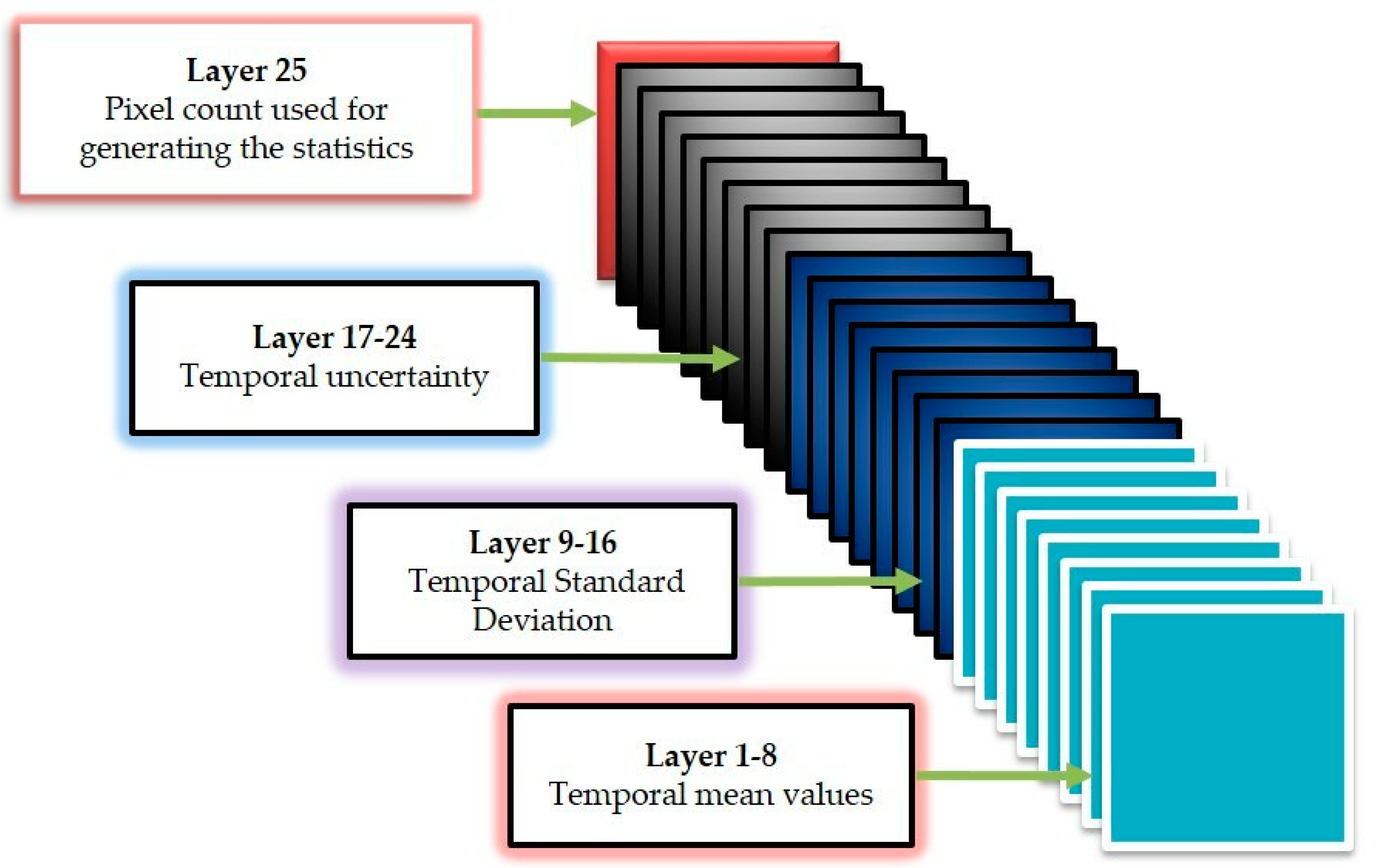
2.2. SDSU Derived Data Product

Landsat 8 OLI data were chosen for this work, as the analyses of Knight et al. [30] and Markham et al. [31] reported an OLI reflectance calibration accuracy of approximately 3%. The key spectral and spatial characteristics of the OLI are presented in

Table 1. Salient characteristics of Landsat-8 Operational Land Imager (OLI).

Wavelength Range	Band Number	Center Wavelength (nm)	Bandwidth (nm)	Spatial Resolution (m)
Coastal	1	443	16	30
Blue	2	492	60	30
Green	3	561	57	30
Red	4	654	37	30
NIR	5	865	28	30
Cirrus	9	1373	20	30
SWIR1	6	1609	85	30
SWIR2	7	2201	187	30
Panchromatic	8	590	172	15

. Through the use of the GEE system, all pixels of North Africa acquired by the OLI over the three-year period were screened for clouds/cloud shadows and saturated pixels. These data were spatially resampled from the native resolution of 30 × 30 meters to 300 × 300 meters. A temporal mean, standard deviation, and uncertainty (ratio of temporal standard deviation to temporal mean) were calculated for each pixel location, along with a count of the number of measurements that went into the statistics calculations. These summary statistics data were then “stacked” into data cubes and “tiled” into 1° latitude by 1° longitude images. The image and pixel sizes were chosen as a practical trade-off between the amount of data retrievable from GEE and the current processing and storage capabilities of the South Dakota State University (SDSU) Image Processing Laboratory systems. In addition, resampling the tiles to 300 m spatial resolution did not significantly degrade the information obtainable from them as much of North Africa is relatively spatially uniform.

Figure 1 shows the concept behind a processed data cube. It consists of 25 layers. Layers 1–8 are the temporal mean statistics image for each VNIR/SWIR multispectral band, ordered by band number starting with the Coastal/Aerosol band and ending with the Cirrus band. Layers 9–16 and 17–24 are the standard deviation and uncertainty images, respectively, again ordered by band number. The final layer consists of the number of resampled image pixels used to calculate the summary statistics.

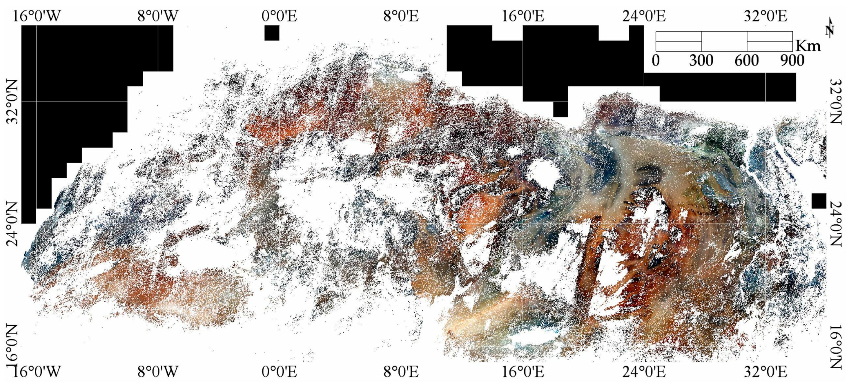
2.3. Mosaic Image of North Africa

Once the processed data tiles were retrieved from GEE and processed locally into data cubes, the temporal mean images were mosaicked to generate composite images of North Africa. The resulting mosaics covered an area from 36°N to 15°N latitude and 18°W to 35°E longitude. In all, approximately 1003 data cubes were used to generate the North Africa mosaics. As part of the mosaicking process, each pixel in a temporal mean tile was screened for a temporal uncertainty of 5% or less, and sufficient resampled pixel count (25 or greater, as it represented approximately one third of the potential cloud-free acquisitions). Helder et al. [2] used a threshold of 3% temporal stability to identify the individual PICS. Since this work focuses on finding continental scale PICS, the temporal variability criteria was relaxed to 5% in order to account for extra variability likely arising due to the large spatial extent of the PICS.

2.4. Classification of North African Land Cover

Landcover maps identifying spectrally similar pixels can be generated through supervised or unsupervised classification algorithms. In supervised classifications (e.g., decision trees, maximum likelihood, and minimum distance [32,33]), reference “training” datasets are used to perform the classification. In unsupervised classifications (e.g., isodata and k-means [34]), standard image processing techniques are directly applied to the image data to perform the classification. There is no consensus regarding the superiority of supervised or unsupervised methods used by themselves; the suitability of the classification method depends on the available reference data. Other research [35,36] suggests that combination of supervised and unsupervised methods can provide more accurate land cover classification results.

This work performs, for the first time, a higher-resolution classification of land cover across all of North Africa. K-means unsupervised classification was chosen as the classification method due to (i) its computational simplicity, which is critical when performing analyses at a continental scale [37,38]; and (ii) the lack of prior knowledge of spectral information for that region. The K-means algorithm is presented below:

• Step 1: Estimate initial mean values for K = 2 clusters:

  $${\displaystyle \sum }_{\mathrm{j}=1}^{\mathrm{NoOfClusters}}{\displaystyle \sum }_{\mathrm{i}=1}^{\mathrm{NoOfBands}}{\mathsf{\mu }}_{\mathrm{ij}}$$

  (1)
• Step 2: Calculate the Euclidean distances between each mosaicked image pixel and initial cluster means:

  $${\displaystyle \sum }_{\mathrm{m}=1,\mathrm{n}=1}^{\mathrm{Row},\mathrm{Column}}{\displaystyle \sum }_{\mathrm{j}=1}^{\mathrm{NoOfClusters}}{\mathrm{D}}_{\mathrm{jmn}}={\displaystyle \sum }_{\mathrm{m}=1,\mathrm{n}=1}^{\mathrm{Row},\mathrm{Column}}{[{\displaystyle \sum }_{\mathrm{j}=1}^{\mathrm{NoOfClusters}}{\displaystyle \sum }_{\mathrm{i}=1}^{\mathrm{NoOfBands}}({\mathrm{x}}_{\mathrm{imn}}-{\mathsf{\mu }}_{\mathrm{ij}})]}^{1/2}$$

  (2)
• Step 3: Classify pixels based on the minimum distance to a cluster:

  $${\sum }_{\mathrm{j}=1}^{\mathrm{NoOfClusters}}{\sum }_{\mathrm{i}=1}^{\mathrm{NoOfBands}}{\mathrm{ClassifiedPixels}}_{\mathrm{ij}}=\min \left({\sum }_{\mathrm{m}=1,\mathrm{n}=1}^{\mathrm{Row},\mathrm{Column}}{\sum }_{\mathrm{j}=1}^{\mathrm{NoOfClusters}}{\mathrm{D}}_{\mathrm{jmn}}\right)$$

  (3)
• Step 4: Calculate the new cluster mean:

  $${\mathsf{\mu }}_{\mathrm{ijnew}}={\displaystyle \sum }_{\mathrm{j}=1}^{\mathrm{NoOfClusters}}{\displaystyle \sum }_{\mathrm{i}=1}^{\mathrm{NoOfBands}}\frac{\mathrm{sum}({\mathrm{ClassifiedPixels}}_{\mathrm{ij}})}{\mathrm{Count}({\mathrm{ClassifiedPixels}}_{\mathrm{ij}})}$$

  (4)
• Step 5: If max(|(${\mathsf{\mu }}_{\mathrm{ij}}-{\mathsf{\mu }}_{\mathrm{ijnew}}$)|) > 0.0001 replace the old cluster mean with the new cluster mean calculated in Step 4, then return to Step 2. Otherwise, proceed to Step 6.
• Step 6: Calculate the spatial uncertainty of all pixels within each cluster.
• Step 7: If the maximum spatial uncertainty of any cluster is greater than 5%, increase the number of clusters by one and return to Step 1. Otherwise, terminate the algorithm.

K-means algorithm was initially “seeded” with cluster means represented by the temporal means of two randomly chosen pixels from the mosaicked images. The Euclidean distance between cluster means (two randomly chosen pixels) and each pixel of the mosaicked image pixels is calculated in Step 2. Third step classifies all the pixels of North Africa based on their minimum distance to the cluster’s mean. The average of the new classified pixels is calculated and considered as the new cluster mean in Step 4. The difference between the current cluster mean and the new cluster mean is computed and if the difference is more than the threshold 0.0001 then current cluster mean is replaced by newly computed cluster mean and again start from Step 2. A mean difference threshold of 0.0001 was used to determine whether new clusters should be created; this threshold value was chosen to ensure that final convergence of the classification remained independent of the chosen starting pixels. For cluster mean differences of less than the difference threshold, the spatial uncertainties of the current set of clusters was calculated. If any cluster’s spatial uncertainty exceeded 5% in any band, the current cluster count was incremented by 1, and the classification process was repeated; otherwise, the classification process terminated at the current cluster count. A 5% spatial uncertainty threshold was selected in order to balance aggregation within cluster regions (i.e., minimizing the creation of smaller cluster regions that are more widely spread) while ensuring lower spatial uncertainty. For this work, the classification process identified 19 distinct clusters.

3. Results and Validation

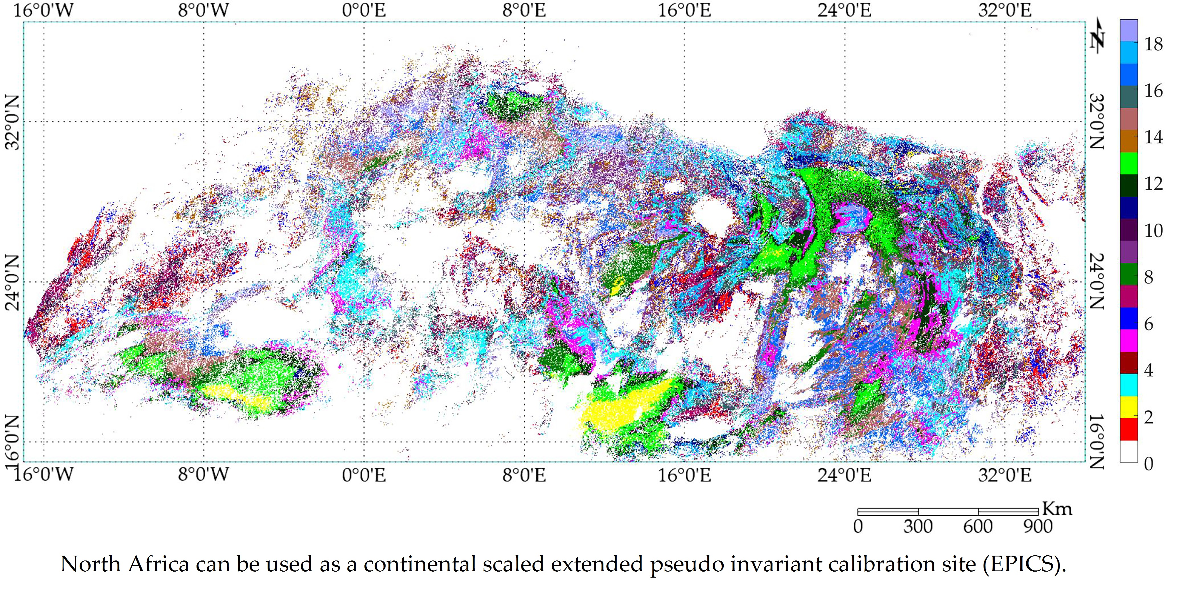
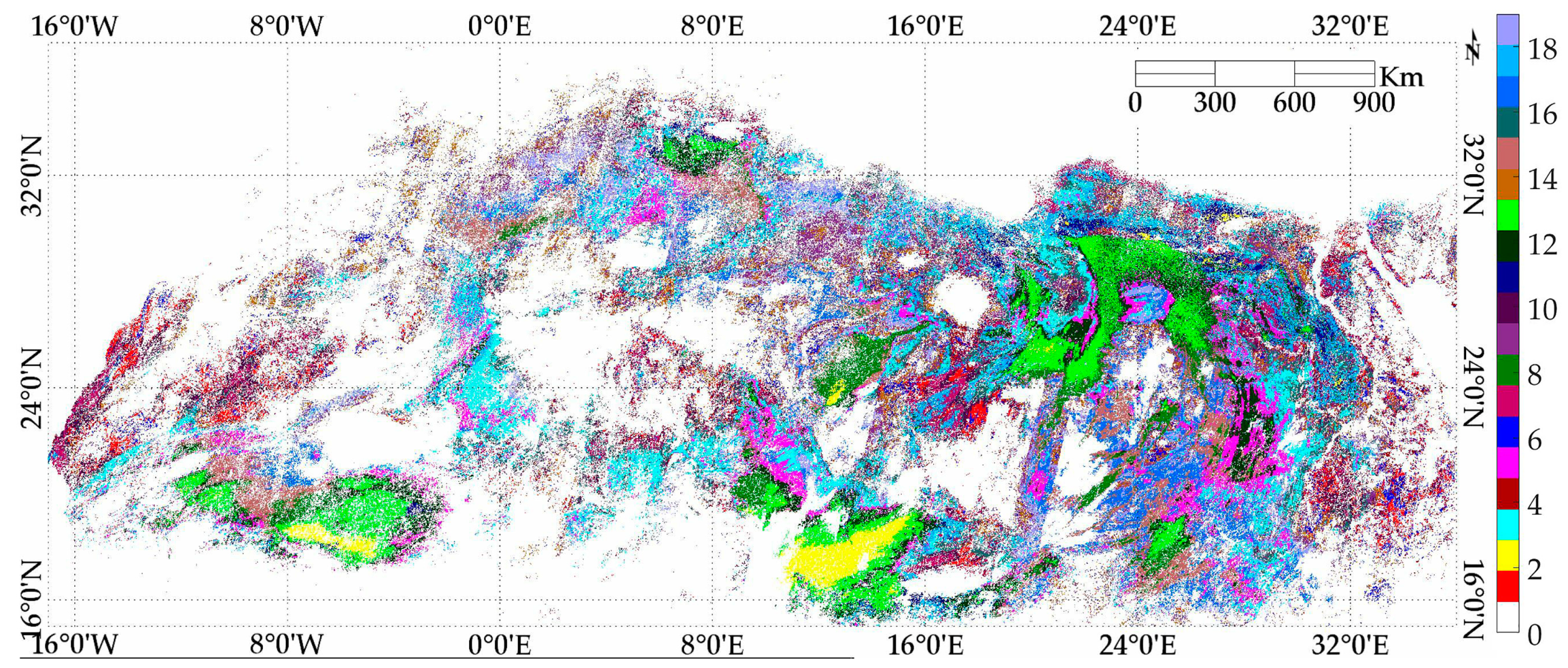
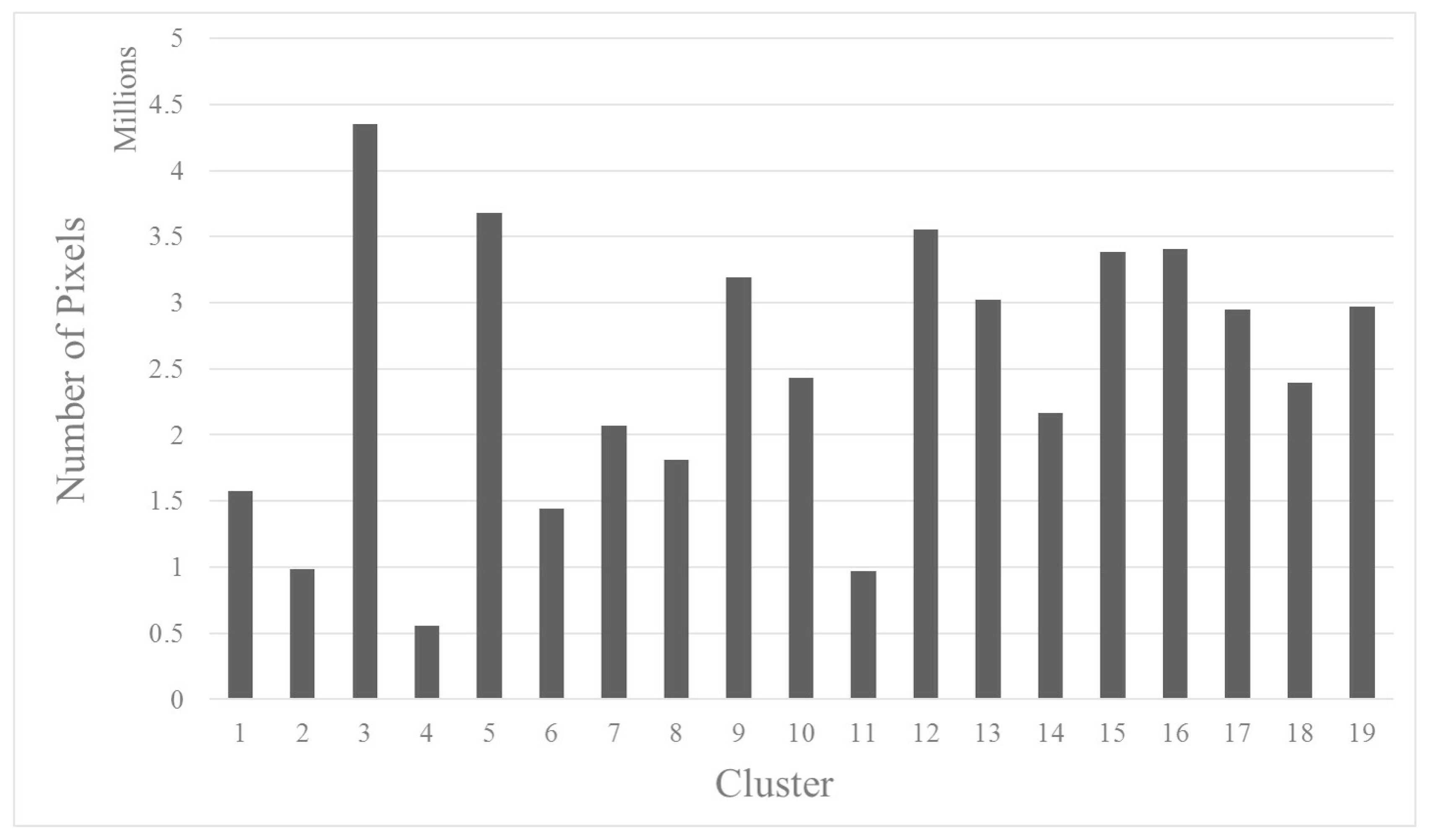
3.1. Classification of North Africa

Figure 2 shows the resulting red/green/blue composite mosaicked image of North Africa after filtering for temporally unstable pixels and pixel count threshold. The white areas represent pixels excluded due to temporal instability and pixels identified as having clouds/cloud shadows and/or small water bodies. The black pixels represent “fill” over regions beyond the African continent.

Figure 3 shows the 19 distinct clusters identified in the classification. All of the identified clusters have contiguous regions widely distributed across the continent, potentially allowing a much higher imaging frequency rather than an imaging frequency of several days for most moderate resolution sensors over a single PICS.

Figure 4 shows a bar graph of the resulting pixel counts for each cluster. Among the clusters, Cluster 3 has the largest number of pixels (approximately 4.3 million). Cluster 13 (the light green graph in Figure 3 has approximately 3 million pixels. Although Cluster 3 has the largest pixel count, its pixels are more widely distributed in non-contiguous regions. The Cluster 13 pixels, on the other hand, are grouped into large contiguous regions widely distributed across North Africa, making this cluster a potential candidate for EPICS-based calibration.

3.2. Spatial Uncertainty of Clusters

Table 2. Cluster Spatial Uncertainties, by Band.

Spatial Uncertainty of Each Cluster of North Africa
Cluster	Coastal	Blue	Green	Red	NIR	SWIR1	SWIR2
1	5.73	6.31	5.37	3.88	3.87	4.14	4.86
2	7.19	7.27	4.83	3.24	2.60	2.06	3.54
3	4.95	5.31	3.94	2.89	2.78	2.36	3.27
4	8.31	9.66	9.82	8.77	8.10	9.67	9.16
5	4.57	4.75	3.44	2.69	2.47	2.23	2.57
6	7.75	8.94	8.03	5.51	5.27	5.89	5.19
7	5.49	5.85	4.68	3.50	3.35	4.05	5.13
8	5.35	5.89	5.03	2.84	2.93	2.54	2.38
9	5.93	6.71	5.67	3.61	3.73	3.19	4.30
10	5.91	6.46	5.21	3.87	3.38	3.37	4.61
11	5.36	5.77	5.07	4.05	3.33	3.45	6.13
12	4.79	5.05	3.34	2.62	2.23	2.03	2.66
13	4.59	4.80	3.08	2.71	2.11	1.78	2.62
14	5.95	6.88	6.38	4.38	4.49	3.87	4.48
15	5.20	5.91	5.16	2.48	2.46	2.15	1.96
16	4.71	5.03	4.02	3.28	2.99	2.95	3.99
17	5.58	6.25	5.28	3.23	3.15	2.53	2.61
18	4.71	4.94	4.14	3.15	2.70	3.15	4.56
19	5.43	6.15	5.39	3.31	3.79	2.88	3.59

shows the final spatial uncertainties (ratio of spatial standard deviation to spatial mean) estimated for each cluster when the classification process was terminated. Due to more pronounced atmospheric scatter in shorter wavelengths, the spatial uncertainties are generally higher in the shorter wavelength bands (the exception being Cluster 4, which exhibited greater uncertainty in the SWIR 1 band). Despite its widespread extent, the Cluster 13 spatial uncertainties are within 5% in the Coastal/Aerosol and Blue bands, and within 3% in the longer wavelength bands. As a result, it should be quite useful for radiometric calibration and radiometric stability assessment.

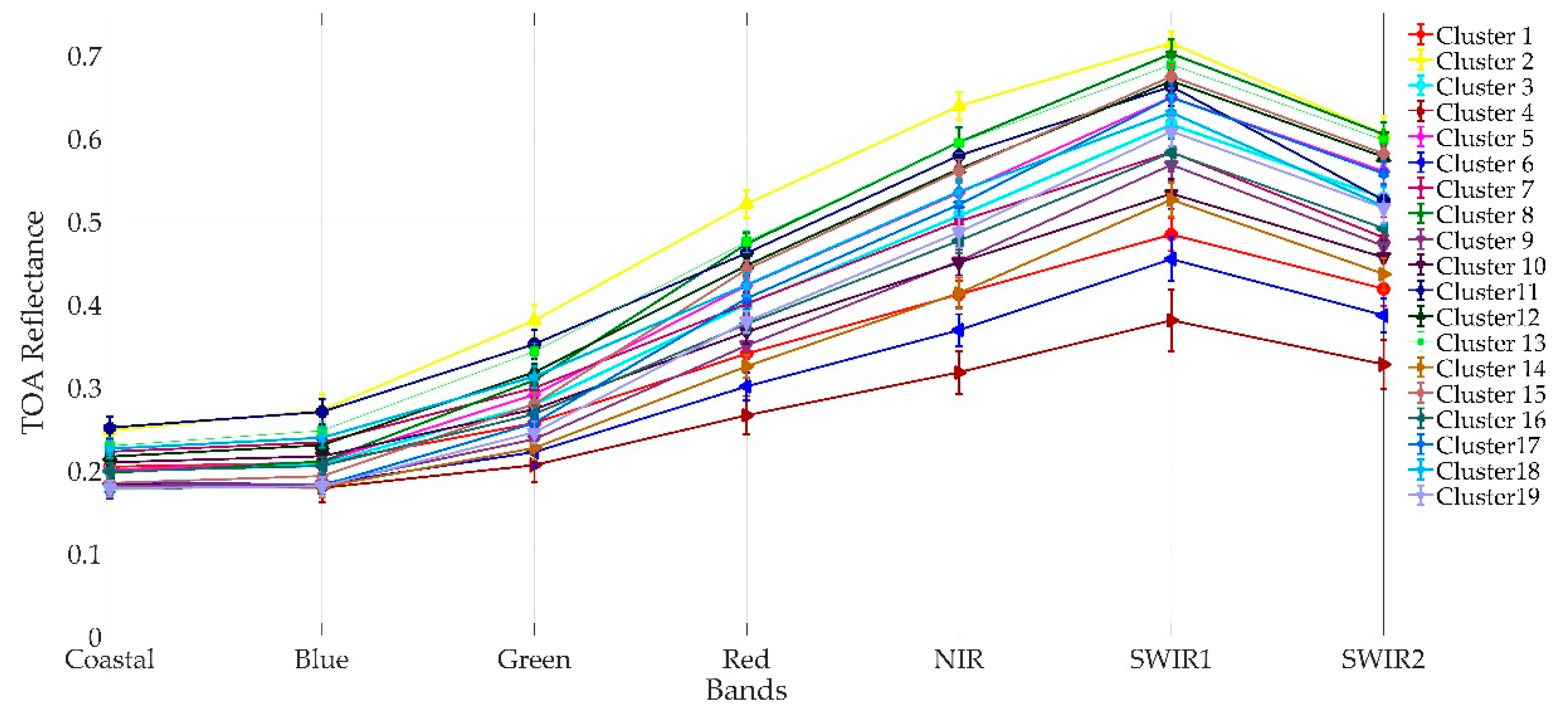
3.3. Cluster Spectral Signatures

Figure 5 shows the multispectral signature of each cluster represented by the mean TOA reflectance and ±1σ standard deviation.

At shorter wavelengths, the surface cover is less reflective; the range of TOA reflectance is narrower, and the standard deviations of different clusters exhibit greater overlap. Conversely, the surface cover is more reflective at longer wavelengths; the range of TOA reflectance is wider, and the standard deviations of different clusters exhibit much less overlap, suggesting that the clusters represent distinct surface cover types.

Cluster 4 (represented by the bottom reddish brown plot) has the lowest overall reflectance levels, while cluster 2 (represented by the top yellow plot) has the highest reflectance levels. This distribution allows sensor calibration across wider portions of the dynamic range, especially at longer wavelengths.

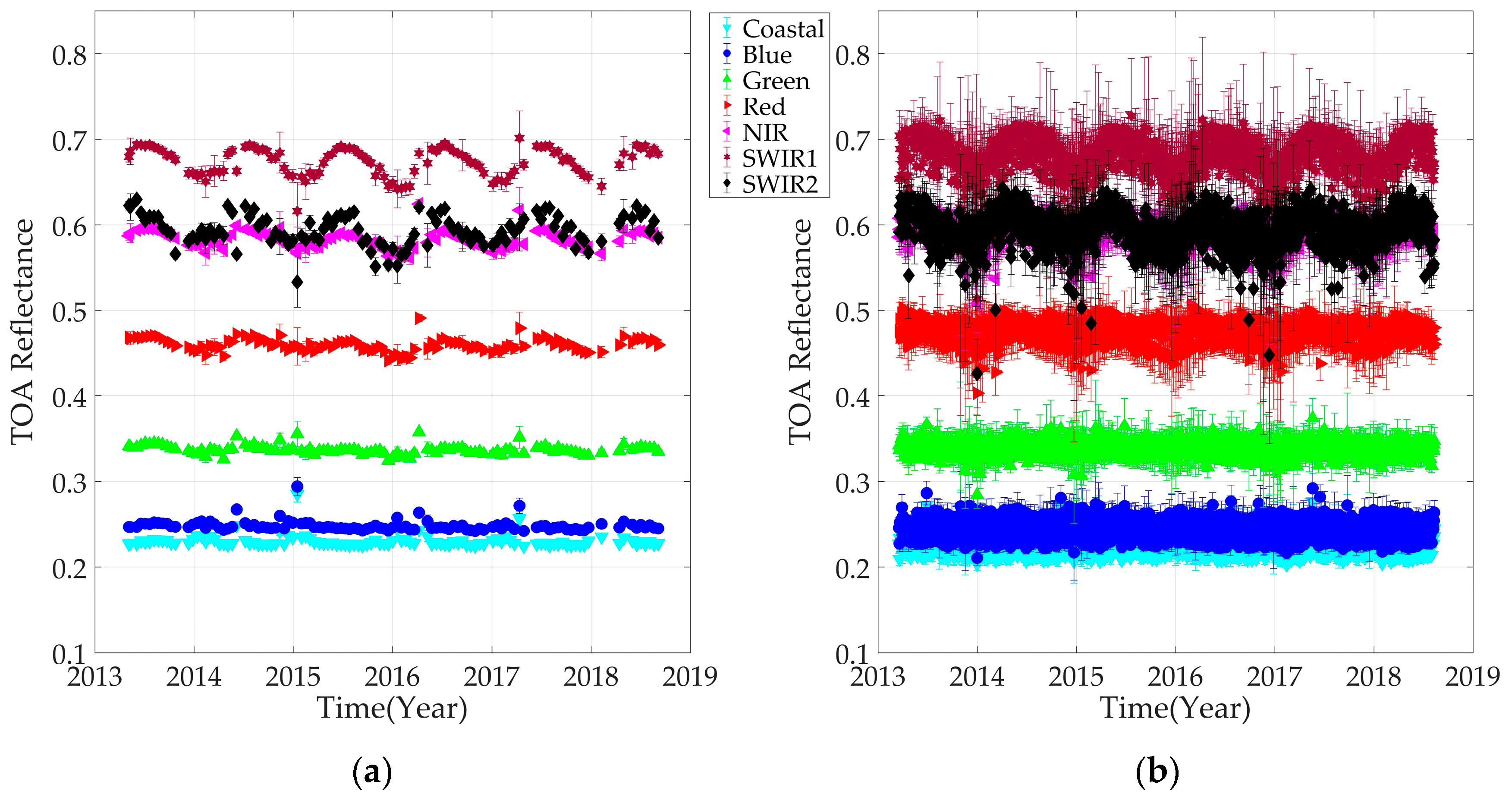
3.4. Comparison of Traditional PICS and Cluster 13 Behaviour

As Cluster 13 spread across the continent, it also includes one of the most widely used traditional PICS i.e., Libya 4, so the temporal behavior of Cluster 13, using selected 16 paths and rows, is compared with Libya 4 temporal behavior as shown in Figure 6. For comparison, Libya 4 CNES (French: Centre national d’études spatiales) region of interest (ROI) is chosen as it is regarded as one of the best regions by CNES based on the long term trending of North African and Arabian desert [2,39]. In Figure 6, the left and right figure present the temporal trend of Libya 4 and Cluster 13, since launch to mid-August 2018, using Landsat 8 OLI. The behavior of Cluster 13 is the same as the behavior of traditional PICS, Libya 4, but it provides a significantly large number of acquisitions than Libya 4 within the same interval of time, i.e., Libya 4 provides 110 could-free observations since launch to mid-August 2018 whereas Cluster 13 provides nearly daily observation and offers 1434 cloud-free observations within the same interval of time. The temporal mean (±2 sigma) of Cluster 13 and Libya 4 are also compared in Figure 7. As Libya 4 temporal mean lies within the uncertainty bar of Cluster 13 temporal mean, the temporal mean of both Libya 4 and Cluster 13 are same. This implies that despite its continental scale spatial extent, Cluster 13 has the same response like the Libya 4 CNES ROI.

3.5. Validation of North African Classification

To validate the North Africa classification results, cloud-free, full-resolution Landsat-7 ETM+ scenes imaging Cluster 13 were obtained. To reduce the amount of data to process, images were limited to 9 distinct WRS-2 path/row combinations from different acquisition dates; these path/row combinations maximized the intersection between the ETM+ images and Cluster 13 region boundaries and provided near-daily imaging frequency during the ETM+’s 16-day revisit period. Binary masks were generated for each path/row image and were used to exclude (i) pixels identified in other clusters; and Cluster 13 pixels with 5% or greater temporal uncertainty. For the purposes of this work, the masks were created at 30 m spatial resolution in order to match the spatial resolution of ETM+; the mask generation procedure is sufficiently general in nature and can generate masks at any required spatial resolution for any sensor.

Figure 8 shows the resulting temporal TOA reflectance trend of Cluster 13 using selected WRS- 2 paths and rows. All the Landsat 7 images used in this analysis were screened for 5% cloud cover due to which the density of Landsat 7 data sample increases after 2014. The error bar of each data points represents its spatial uncertainty. The cluster means, spatial uncertainty, temporal uncertainty and the corresponding statistics from the temporal trend are listed in

Table 3. Comparison of K-Means Cluster 13 Statistics and Scene-Based Cluster 13 Statistics.

Cluster 13	K Means Algorithm			Selected Landsat 7 Scenes
Band	Mean	Spatial Uncertainty (%)	Temporal Uncertainty (%)	Mean	Spatial Uncertainty (%)	Temporal Uncertainty (%)
Coastal	0.23	4.59	5.00	N/A	N/A	N/A
Blue	0.25	4.80	5.00	0.25	4.82	3.96
Green	0.34	3.08	5.00	0.34	4.30	2.22
Red	0.47	2.71	5.00	0.47	4.13	2.86
NIR	0.59	2.11	5.00	0.60	4.07	2.88
SWIR1	0.69	1.78	5.00	0.69	4.09	2.85
SWIR2	0.60	2.62	5.00	0.60	4.41	3.65

. The overall cluster means and temporal trend from different WRS2 paths and rows are essentially the same for most of the band except NIR band where there is an offset of 0.01 reflectance unit. The lifetime time series of Cluster 13 TOA reflectance using Landsat 7 shows a trend in some bands and also exhibits apparent seasonal effects in the longer wavelength bands, indicating the necessity for additional drift and BRDF correction. It is possible that the observed reflectance differences are due to (i) no application of BRDF correction to the data; (ii) no application of drift correction to the data, and (iii) potential outliers in the data. As mentioned earlier, all pixels used as input to the K-means algorithm exhibited temporal uncertainties of 5% or less. Not surprisingly, the Cluster 13 trend data also exhibits approximately 5% or less temporal uncertainty.

In general, the image-estimated spatial uncertainties are larger than the corresponding classification-estimated spatial uncertainties; however, they are within 5% in all bands. The large image-estimated spatial uncertainty is due to the reason that the selected path/row images intersect sub-regions within Cluster 13 exhibiting more heterogeneous reflectance values, resulting in a larger standard deviation and corresponding spatial uncertainty.

4. Discussion

This work has developed a novel procedure for classification of Landsat-8 OLI image data of North Africa, demonstrating the region’s potential for use as an extended PICS. The classification, based on a standard k-means unsupervised classification, is computationally simple and does not require prior knowledge of the region’s spectral characteristics. The proposed procedure allows efficient storage and processing of large amounts of OLI image data by resampling them to 300 m spatial resolution; due to the relative uniformity of the region, resampling does not lead to significant loss of spectral information that would adversely impact the resulting classification. The procedure relies on a maximum 5% temporal uncertainty threshold to account for additional variability resulting from use of a much larger region size. Overall, the proposed procedure represents a significant advance over previous efforts that relied heavily upon visual inspection to identify much smaller candidate PICS regions [2,24], and can be applied “as is” to any sensor. The proposed procedure identified 19 distinct “clusters” of pixels exhibiting temporal uncertainty of 5% or less. Processing in the procedure terminated when the spatial uncertainty within any given cluster was 5% or less across all bands. The 5% spatial uncertainty threshold represents a practical compromise to avoid the extremes of (i) lower spatial uncertainty within a larger number of clusters; or (ii) higher spatial uncertainty within a smaller number of clusters, either of which would yield a less accurate calibration.

Previous landcover classifications had identified North Africa as “barren”, containing less than 10% vegetation and composed primarily of some combination of sand, bare soil, and rock [27,28,40]. The “barren” classification has largely remained to the present time, as the scientific community did not demand a finer classification. However, this landcover classification applies to many current PICS extensively used for sensor radiometric calibration and performance analysis, such as Libya 4, Mauritania 1, and Algeria 1 [5,8,21,22]. Choi et al. [41] studied the spectral stability of the Libya 4, Libya 1 and Mauritania 2 PICS using average deviation (AD) and spectral angle mapper (SAM) where average deviation is the absolute reflectance difference and SAM is the spectral angle between the test and reference spectrum [42,43]. This is the earliest attempt to study the spectral similarity of PICS and in this study, they found that ROIs chosen parallel to the along-track direction were spectrally stable for spectral angle mapper values up to ±2 degrees, with an average deviation of ±1.7% in reflectance scale. In contrast to previous work, this work presents the classification of North Africa by studying each and every pixel and group together the pixels with similar characteristics in order to develop extended pseudo invariant calibration sites.

Clusters found by the unsupervised classification algorithm possess different spectral characteristics. Even if the spectral signature of clusters appears to be similar in multiple bands, they are distinct if they are observed across all the bands. The spectral separation between different clusters is wavelength dependent, as shown in Figure 5. Longer wavelengths have very distinct spectral separation; the SWIR1 band has the most distinct spectral separation of 0.33 reflectance units whereas the coastal band has poor spectral separation, just separated by 0.07 reflectance units. So, on the basis of different intensity levels, North Africa offers a better dynamic range for sensor calibration at longer wavelengths than at shorter wavelengths as shown in Figure 5.

Factors to consider when performing a cluster-based analysis include the cluster size (represented by the number of pixels in the cluster) and its distribution across a region, as well as the degree of contiguity of the cluster pixels. The “optimal” cluster for calibration and performance monitoring balances a lower spatial uncertainty, a larger size and distribution (in order to cover a larger geographic area), and a greater degree of pixel contiguity (in order to minimize effects due to geometric misregistration between images); this becomes particularly important for sensors with higher (<30 m) spatial resolution.

Two of the clusters identified by the proposed procedure (Clusters 2 and 3) exhibit similar levels of spatial uncertainty at longer wavelengths. With respect to cluster size and distribution across the region, Cluster 3 would be considered optimal; however, with respect to cluster contiguity, Cluster 2 would be considered optimal. For sensors with lower geometric accuracy, Cluster 2 would be preferred for radiometric calibration and sensor performance analysis.

Cluster 3 has the largest number of pixels (approximately 4.3 million) as shown in Figure 4, however, as mentioned above, its pixels are relatively non-contiguous. In contrast, Cluster 13 possesses a similar intensity level to Cluster 3, and contains a slightly smaller number of pixels that are almost as widely distributed across northern Africa. However, its spatial uncertainty is smaller than Cluster 3’s across most bands, and its pixels form much more contiguous subregions. While other clusters might be preferable to Cluster 13 with respect to spatial uncertainty and cluster characteristics in specific bands (e.g., Clusters 5 and 15 in the Red and SWIR2 bands), Cluster 13 exhibits favorable characteristics across the majority of bands, making it an ideal bright target cluster for calibration purposes.

Similarly, Clusters 4 and 6 provide a lower intensity level that would help widen the dynamic range for PICS based calibration. Between them, Cluster 4 is slightly darker, but it has a spatial uncertainty of approximately 8% to 9% across all bands; in addition, it contains the smaller number of pixels forming less contiguous subregions. Cluster 6 would be preferred due to its larger number of pixels, more contiguous sub-regions and lower spatial uncertainty.

Some of the key advantages that this classification of North Africa offered to the radiometric calibration community are highlighted as follows:

• Historically, PICS-based calibration work used bright desert targets due to there being no universally recognized set of darker PICS exhibiting sufficient temporal and spatial stability. As the proposed procedure identifies clusters with 5% or better temporal stability, it offers the potential for improving calibration accuracy by extending the dynamic range over which calibration can be performed.
• Previously, PICS such as Libya 4 has only one image acquisition corresponding to the satellite revisit cycle but Cluster 13 found by the classification of North Africa is observed in nearly a daily fashion. As Libya 4 lies within Cluster 13, it is similar to observing Libya 4 in a daily manner in contrast to 16 days’ period which helps to quickly detect the drift of any satellite sensors with greater sensitivity.
• One of the major application of PICS is the cross-calibration of optical satellite sensors [14,16,44]. Previously, limited cross calibration opportunities were available as PICS are observed once in 16 days. However, Cluster 13 provides more cross-calibration opportunities as it spreads across the continent which helps to decrease the cross-calibration gain and bias uncertainties between any optical satellite sensor pairs. In addition, it helps to achieve a cross calibration quality similar to that of individual PICS in a significantly shorter time interval.
• Several researchers have developed data driven absolute calibration model in order to simulate the TOA reflectance of an individual PICS, such as Libya 4 [19,20,21,22,23]. The number of Libya 4 observations is limited due to orbital pattern and cloud cover. As Cluster 13 has a significantly large number of observations than an individual PICS, it enhances the model’s ability to predict the TOA reflectance more accurately as more training datasets are available for developing the EPICS based absolute calibration model. Furthermore, EPICS based absolute calibration model can increase the temporal resolution of calibration opportunities to a daily or nearly daily basis for any optical satellite sensor.

This paper only presents initial cluster classification results. Since Cluster 13 has more than 3 million pixels, offers lower spatial uncertainty across most bands, and forms more contiguous subregions widely distributed across North Africa, it stands out as a viable first candidate for EPICS based calibration. Future directions for this work would investigate the use of cluster regions, beginning with Cluster 13, to perform long-term stability assessment and sensor cross calibration. The following sections discuss these potential cluster-based applications in greater detail.

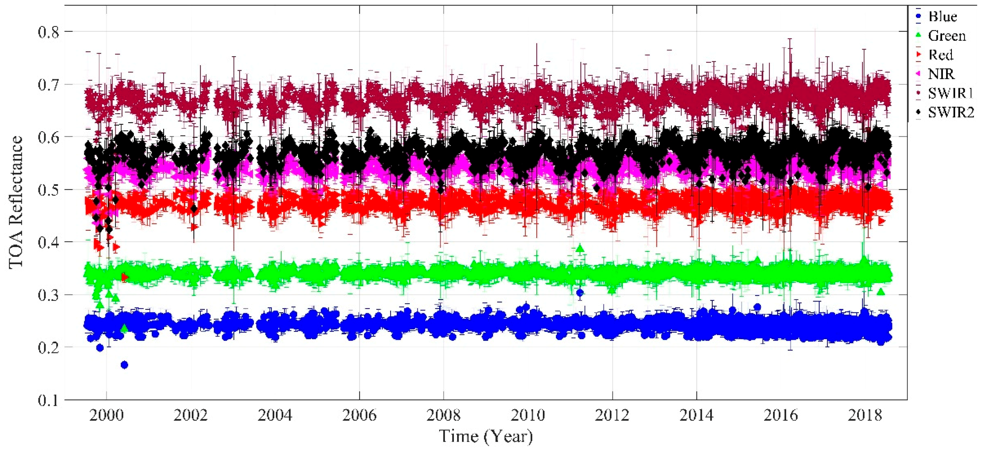
4.1. Long Term Monitoring of Sensor Radiometric Stability

Cluster-based analyses of long-term sensor stability can potentially benefit from a significant increase in temporal resolution over that provided by individual PICS, since a cluster is considered as a group of spectrally similar pixels, with each cluster containing contiguous regions distributed across the continent. Preliminary investigation into this topic has begun with Cluster 13, as its contiguous regions tended to be the largest in size among all the clusters and were more widely distributed. Figure 9 shows the intersection of Landsat WRS-2 path/rows (black lines) and Cluster 13 region boundaries (red). In all, 25 WRS-2 path/rows imaging these regions were identified, potentially allowing multiple image acquisitions per day within the 16-day revisit period. This potential increase in temporal resolution could result in quicker detection of sensor response changes over time, which would be especially desirable for sensors with shorter life expectancies and greater variability in detector response.

4.2. Hyperspectral Data Availability for Cross Calibration

A cluster-based cross calibration approach would need to have accurate knowledge of the cluster’s expected hyperspectral response, in order to derive appropriate scaling factors to compensate for spectral response differences between a well calibrated “reference” sensor and the sensor to be calibrated. In the absence of ground truth measurements, this knowledge can be derived from available hyperspectral image data. Figure 10 shows a simplified diagram of the five largest contiguous regions of Cluster 13 across North Africa (represented by the blue color) and a map of the available Hyperion coverage over the same regions (represented by the red color). Hyperion is a hyperspectral pushbroom sensor imaging the Earth’s surface in the 400–2500 nm portion of the solar spectrum, in 242 overlapping bands with a spectral resolution of approximately 10 nm; 196 of these bands are well calibrated. It images a 7 km by 100 km swath at a spatial resolution of 30 m [45,46,47,48]. Preliminary investigation has identified a set of 731 Hyperion scenes imaging these regions. After filtering the set for 10% or less cloud cover and sensor view angles within ± 5° of nadir, 101 scenes were identified that could be used to determine the hyperspectral profile. As Cluster 13 regions are spectrally similar (as determined by the classification process), it could be expected that the hyperspectral profile of a region may be used as a “representative” profile for the entire cluster.

5. Conclusions

This work demonstrated the potential of using the whole of North Africa as a continental PICS. Traditionally, only a few locations in North Africa have been used due to the lack of knowledge about the temporal stability of most of North Africa. This work analyzed each and every pixel of North Africa and found that the majority of North Africa is temporally stable and could potentially be used for the radiometric calibration of satellite sensors.

Conventionally, all these pixels were broadly categorized as a “barren” surface type which includes soil, sand, and rock. This work developed a first-ever high-resolution classification of this “barren” surface type of North Africa using Landsat 8 OLI image data and sub classified it into finer classes using an unsupervised classification algorithm. The algorithm identified 19 clusters each representing a distinct surface type having different spectral characteristics. The range of TOA reflectance at shorter wavelengths is narrow, but wider at longer wavelengths which offers a wide dynamic range to calibrate optical satellite sensors.

All of the identified clusters contained a large number of pixels grouped in contiguous regions potentially useable for sensor calibration and stability assessment. Among all the clusters, Cluster 13 possessed the largest contiguous region, lowest overall spatial uncertainty and was also more widely distributed across North Africa. Due to their spatial extent, most of the clusters allowed multiple imaging opportunities per day in contrast to a typical once during the sensor’s revisit time. Multiple imaging opportunities obtained through a cluster, or EPICS, approach increases the temporal resolution of a calibration time series which leads to increased sensitivity for quicker identification of changes in sensor response.

While some obvious next steps need to take place, as indicated in the discussion sections, the results presented in this paper are very promising. They represent an advance towards the development of an extended PICS (EPICS) with large areal extent, and the ability to evaluate any sensor system on a daily basis using a potentially continent-wide site that behaves as a point site. The cluster-based approach could lead to a new way to calibrate and monitor sensor radiometric performance on orbit. More importantly, this approach could address a very new and serious problem of calibration monitoring for shorter-lived sensor missions, such as low-cost small satellite-based systems, where more pronounced degradation in radiometric performance is possible.

References

1. Six, D.; Fily, M.; Alvain, S.; Henry, P.; Benoist, J.-P. Surface characterisation of the Dome Concordia area (Antarctica) as a potential satellite calibration site, using Spot 4/Vegetation instrument. Remote Sens. Environ. 2004, 89, 83–94. [Google Scholar] [CrossRef]
2. Helder, D.L.; Basnet, B.; Morstad, D.L. Optimized identification of worldwide radiometric pseudo-invariant calibration sites. Can. J. Remote Sens. 2010, 36, 527–539. [Google Scholar] [CrossRef]
3. Teillet, P.; Chander, G. Terrestrial reference standard sites for postlaunch sensor calibration. Can. J. Remote Sens. 2010, 36, 437–450. [Google Scholar] [CrossRef]
4. Teillet, P.; Barsi, J.; Chander, G.; Thome, K. Prime candidate earth targets for the post-launch radiometric calibration of space-based optical imaging instruments. In Proceedings of the Earth Observing Systems XII, San Diego, CA, USA, 26–30 August 2007; p. 66770S. [Google Scholar]
5. Chander, G.; Xiong, X.J.; Choi, T.J.; Angal, A. Monitoring on-orbit calibration stability of the Terra MODIS and Landsat 7 ETM+ sensors using pseudo-invariant test sites. Remote Sens. Environ. 2010, 114, 925–939. [Google Scholar] [CrossRef]
6. Kim, W.; He, T.; Wang, D.; Cao, C.; Liang, S. Assessment of long-term sensor radiometric degradation using time series analysis. IEEE Trans. Geosci. Remote Sens. 2014, 52, 2960–2976. [Google Scholar] [CrossRef]
7. Angal, A.; Chander, G.; Xiong, X.; Choi, T.J.; Wu, A. Characterization of the Sonoran desert as a radiometric calibration target for Earth observing sensors. J. Appl. Remote Sens. 2011, 5, 059502. [Google Scholar] [CrossRef] [Green Version]
8. Angal, A.; Xiong, X.; Choi, T.; Chander, G.; Wu, A. Using the Sonoran and Libyan Desert test sites to monitor the temporal stability of reflective solar bands for Landsat 7 enhanced thematic mapper plus and Terra moderate resolution imaging spectroradiometer sensors. J. Appl. Remote Sens. 2010, 4, 043525. [Google Scholar] [CrossRef]
9. Smith, D.L.; Mutlow, C.T.; Rao, C.N. Calibration monitoring of the visible and near-infrared channels of the Along-Track Scanning Radiometer-2 by use of stable terrestrial sites. Appl. Opt. 2002, 41, 515–523. [Google Scholar] [CrossRef] [PubMed]
10. Li, C.; Xue, Y.; Liu, Q.; Guang, J.; He, X.; Zhang, J.; Wang, T.; Liu, X. Post calibration of channels 1 and 2 of long-term AVHRR data record based on SeaWiFS data and pseudo-invariant targets. Remote Sens. Environ. 2014, 150, 104–119. [Google Scholar] [CrossRef]
11. Doelling, D.R.; Wu, A.; Xiong, X.; Scarino, B.R.; Bhatt, R.; Haney, C.O.; Morstad, D.; Gopalan, A. The radiometric stability and scaling of collection 6 Terra-and Aqua-MODIS VIS, NIR, and SWIR spectral bands. IEEE Trans. Geosci. Remote Sens. 2015, 53, 4520–4535. [Google Scholar] [CrossRef]
12. Chander, G.; Meyer, D.J.; Helder, D.L. Cross calibration of the Landsat-7 ETM+ and EO-1 ALI sensor. IEEE Trans. Geosci. Remote Sens. 2004, 42, 2821–2831. [Google Scholar] [CrossRef]
13. Chander, G.; Angal, A.; Choi, T.J.; Meyer, D.J.; Xiong, X.J.; Teillet, P.M. Cross-calibration of the Terra MODIS, Landsat 7 ETM+ and EO-1 ALI sensors using near-simultaneous surface observation over the Railroad Valley Playa, Nevada, test site. In Proceedings of the Earth Observing Systems XII, San Diego, CA, USA, 26–30 August 2007; p. 66770Y. [Google Scholar]
14. Chander, G.; Angal, A.; Choi, T.; Xiong, X. Radiometric cross-calibration of EO-1 ALI with L7 ETM+ and Terra MODIS sensors using near-simultaneous desert observations. IEEE J. Sel. Top. Appl. Earth Obs. Remote Sens. 2013, 6, 386–399. [Google Scholar] [CrossRef]
15. Pinto, C.; Ponzoni, F.; Castro, R.; Leigh, L.; Mishra, N.; Aaron, D.; Helder, D. First in-flight radiometric calibration of MUX and WFI on-board CBERS-4. Remote Sens. 2016, 8, 405. [Google Scholar] [CrossRef]
16. Mishra, N.; Haque, M.O.; Leigh, L.; Aaron, D.; Helder, D.; Markham, B. Radiometric cross calibration of Landsat 8 operational land imager (OLI) and Landsat 7 enhanced thematic mapper plus (ETM+). Remote Sens. 2014, 6, 12619–12638. [Google Scholar] [CrossRef]
17. Li, S.; Ganguly, S.; Dungan, J.L.; Wang, W.; Nemani, R.R. Sentinel-2 MSI radiometric characterization and cross-calibration with Landsat-8 OLI. Adv. Remote Sens. 2017, 6, 147. [Google Scholar] [CrossRef]
18. Govaerts, Y.M.; Clerici, M. Evaluation of radiative transfer simulations over bright desert calibration sites. IEEE Trans. Geosci. Remote Sens. 2004, 42, 176–187. [Google Scholar] [CrossRef]
19. Govaerts, Y.; Sterckx, S.; Adriaensen, S. Optical sensor calibration using simulated radiances over desert sites. In Proceedings of the 2012 IEEE International Geoscience and Remote Sensing Symposium (IGARSS), Munich, Germany, 22–27 July 2012; pp. 6932–6935. [Google Scholar]
20. Govaerts, Y.; Sterckx, S.; Adriaensen, S. Use of simulated reflectances over bright desert target as an absolute calibration reference. Remote Sens. Lett. 2013, 4, 523–531. [Google Scholar] [CrossRef]
21. Mishra, N.; Helder, D.; Angal, A.; Choi, J.; Xiong, X. Absolute calibration of optical satellite sensors using Libya 4 pseudo invariant calibration site. Remote Sens. 2014, 6, 1327–1346. [Google Scholar] [CrossRef]
22. Helder, D.; Thome, K.J.; Mishra, N.; Chander, G.; Xiong, X.; Angal, A.; Choi, T. Absolute radiometric calibration of Landsat using a pseudo invariant calibration site. IEEE Trans. Geosci. Remote Sens. 2013, 51, 1360–1369. [Google Scholar] [CrossRef]
23. Bouvet, M. Radiometric comparison of multispectral imagers over a pseudo-invariant calibration site using a reference radiometric model. Remote Sens. Environ. 2014, 140, 141–154. [Google Scholar] [CrossRef]
24. Cosnefroy, H.; Leroy, M.; Briottet, X. Selection and characterization of Saharan and Arabian desert sites for the calibration of optical satellite sensors. Remote Sens. Environ. 1996, 58, 101–114. [Google Scholar] [CrossRef]
25. Tabassum, R. Worldwide Optimal Pics Search; South Dakota State University: Brookings, SD, USA, 2017. [Google Scholar]
26. Loveland, T.; Merchant, J.; Brown, J.; Ohlen, D. Development of a land-cover characteristics database for the conterminous U. S. Photogramm. Eng. Remote Sens. 1991, 57, 1453–1463. [Google Scholar]
27. Hansen, M.C.; DeFries, R.S.; Townshend, J.R.; Sohlberg, R. Global land cover classification at 1 km spatial resolution using a classification tree approach. Int. J. Remote sens. 2000, 21, 1331–1364. [Google Scholar] [CrossRef] [Green Version]
28. Friedl, M.A.; McIver, D.K.; Hodges, J.C.; Zhang, X.; Muchoney, D.; Strahler, A.H.; Woodcock, C.E.; Gopal, S.; Schneider, A.; Cooper, A. Global land cover mapping from MODIS: Algorithms and early results. Remote Sens. Environ. 2002, 83, 287–302. [Google Scholar] [CrossRef]
29. Gorelick, N.; Hancher, M.; Dixon, M.; Ilyushchenko, S.; Thau, D.; Moore, R. Google Earth Engine: Planetary-scale geospatial analysis for everyone. Remote Sens. Environ. 2017, 202, 18–27. [Google Scholar] [CrossRef]
30. Knight, E.J.; Kvaran, G. Landsat-8 operational land imager design, characterization and performance. Remote Sens. 2014, 6, 10286–10305. [Google Scholar] [CrossRef]
31. Markham, B.; Barsi, J.; Kvaran, G.; Ong, L.; Kaita, E.; Biggar, S.; Czapla-Myers, J.; Mishra, N.; Helder, D. Landsat-8 operational land imager radiometric calibration and stability. Remote Sens. 2014, 6, 12275–12308. [Google Scholar] [CrossRef]
32. Lu, D.; Weng, Q. A survey of image classification methods and techniques for improving classification performance. Int. J. Remote Sens. 2007, 28, 823–870. [Google Scholar] [Green Version]
33. Hurd, J.D.; Civco, D.L. Creating an image dataset to meet your classification needs: A proof-of-concept study. In Proceedings of the ASPRS Annual Conference, Baltimore, MD, USA, 9–13 March 2009. [Google Scholar]
34. Kanniah, K.D.; Wai, N.S.; Shin, A.; Rasib, A.W. Per-pixel and sub-pixel classifications of high-resolution satellite data for mangrove species mapping. Appl. GIS 2007, 3, 1–22. [Google Scholar]
35. Castellana, L.; D’Addabbo, A.; Pasquariello, G. A composed supervised/unsupervised approach to improve change detection from remote sensing. Pattern Recognit. Lett. 2007, 28, 405–413. [Google Scholar] [CrossRef]
36. Rozenstein, O.; Karnieli, A. Comparison of methods for land-use classification incorporating remote sensing and GIS inputs. Appl. Geogr. 2011, 31, 533–544. [Google Scholar] [CrossRef]
37. Pelleg, D.; Moore, A.W. X-means: Extending k-means with efficient estimation of the number of clusters. In Proceedings of the Seventeenth International Conference on Machine Learning ICML, Stanford, CA, USA, 29 June–2 July 2000; pp. 727–734. [Google Scholar]
38. Kanungo, T.; Mount, D.M.; Netanyahu, N.S.; Piatko, C.D.; Silverman, R.; Wu, A.Y. A local search approximation algorithm for k-means clustering. Comput. Geom. 2004, 28, 89–112. [Google Scholar] [CrossRef] [Green Version]
39. Chander, G.; Mishra, N.; Helder, D.L.; Aaron, D.B.; Angal, A.; Choi, T.; Xiong, X.; Doelling, D.R. Applications of spectral band adjustment factors (SBAF) for cross-calibration. IEEE Trans. Geosci. Remote Sens. 2013, 51, 1267–1281. [Google Scholar] [CrossRef]
40. Loveland, T.R.; Reed, B.C.; Brown, J.F.; Ohlen, D.O.; Zhu, Z.; Yang, L.; Merchant, J.W. Development of a global land cover characteristics database and IGBP DISCover from 1 km AVHRR data. Int. J. Remote Sens. 2000, 21, 1303–1330. [Google Scholar] [CrossRef] [Green Version]
41. Choi, T.J.; Xiong, X.; Angal, A.; Chander, G.; Qu, J.J. Assessment of the spectral stability of Libya 4, Libya 1, and Mauritania 2 sites using Earth Observing One Hyperion. J. Appl. Remote Sens. 2014, 8, 083618. [Google Scholar] [CrossRef]
42. Kruse, F.A.; Lefkoff, A.; Boardman, J.; Heidebrecht, K.; Shapiro, A.; Barloon, P.; Goetz, A. The spectral image processing system (SIPS)—Interactive visualization and analysis of imaging spectrometer data. Remote Sens. Environ. 1993, 44, 145–163. [Google Scholar] [CrossRef]
43. Yuhas, R.H.; Goetz, A.F.; Boardman, J.W. Discrimination among Semi-Arid landscape Endmembers Using the Spectral Angle Mapper (SAM) Algorithm. 1992. Available online: https://ntrs.nasa.gov/search.jsp?R=19940012238 (accessed on 3 April 2019).
44. Angal, A.; Xiong, X.; Wu, A.; Chander, G.; Choi, T. Multitemporal cross-calibration of the Terra MODIS and Landsat 7 ETM+ reflective solar bands. IEEE Trans. Geosci. Remote Sens. 2013, 51, 1870–1882. [Google Scholar] [CrossRef]
45. Folkman, M.A.; Pearlman, J.; Liao, L.B.; Jarecke, P.J. EO-1/Hyperion hyperspectral imager design, development, characterization, and calibration. In Proceedings of the Hyperspectral Remote Sensing of the Land and Atmosphere, Sendai, Japan, 9–12 October 2000; pp. 40–52. [Google Scholar]
46. Pearlman, J.; Segal, C.; Liao, L.B.; Carman, S.L.; Folkman, M.A.; Browne, W.; Ong, L.; Ungar, S.G. Development and operations of the EO-1 Hyperion imaging spectrometer. In Proceedings of the Earth Observing Systems V, San Diego, CA, USA, 30 July–4 August 2000; pp. 243–254. [Google Scholar]
47. Ungar, S.G.; Pearlman, J.S.; Mendenhall, J.A.; Reuter, D. Overview of the earth observing one (EO-1) mission. IEEE Trans. Geosci. Remote Sens. 2003, 41, 1149–1159. [Google Scholar] [CrossRef]
48. Pearlman, J.S.; Barry, P.S.; Segal, C.C.; Shepanski, J.; Beiso, D.; Carman, S.L. Hyperion, a space-based imaging spectrometer. IEEE Trans. Geosci. Remote Sens. 2003, 41, 1160–1173. [Google Scholar] [CrossRef]
Figure 1. SDSU Data Tile Layers Derived from Google Earth Engine (GEE).
Remotesensing 11 00875 g001
Figure 2. North Africa Mosaic After Filtering Temporally Unstable Pixels.
Remotesensing 11 00875 g002
Figure 3. K-Means Classification of North Africa to 5% Spatial Uncertainty.
Remotesensing 11 00875 g003
Figure 4. Number of pixels in each North African cluster.
Remotesensing 11 00875 g004
Figure 5. Spectral Signature of Clusters, by Band.
Remotesensing 11 00875 g005
Figure 6. Comparison between traditional PICS (Libya 4) (a) and Cluster 13 (b) behavior. Figures (a,b) show the trending of Libya 4 and Cluster 13, as a function of time since launch to August 2018, using Landsat 8 OLI.
Remotesensing 11 00875 g006
Figure 7. Comparison between the temporal mean and its standard deviation between traditional PICS (Libya 4 CNES ROI) and Cluster 13. Red and Blue symbols represent the temporal mean of Libya 4 CNES ROI and Cluster 13 respectively.
Remotesensing 11 00875 g007
Figure 8. Lifetime OLI TOA Reflectance of Cluster 13 using Landsat 7, No BRDF Correction.
Remotesensing 11 00875 g008
Figure 9. Cluster 13 coverage over North Africa and corresponding WRS2 paths and rows.
Remotesensing 11 00875 g009
Figure 10. Cluster 13 Extent Across North Africa with Corresponding Hyperion Coverage.
Remotesensing 11 00875 g010