Shallow Landslide Prediction Using a Novel Hybrid Functional Machine Learning Algorithm

 ,
,  , , , ,
  ,
,  ,
,  , ,
, ,  , , and
Abstract
:
1. Introduction
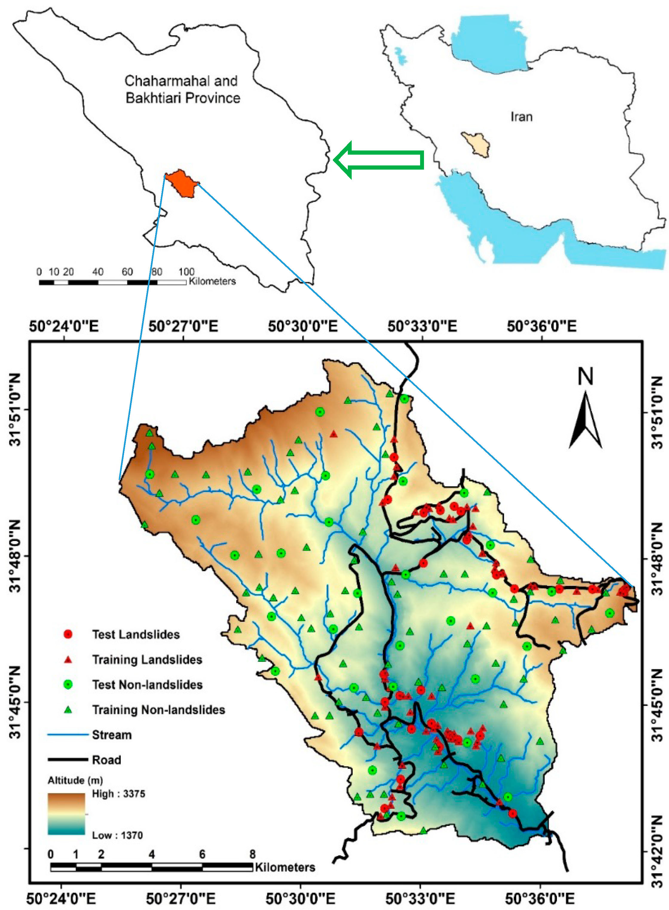
2. Study Area
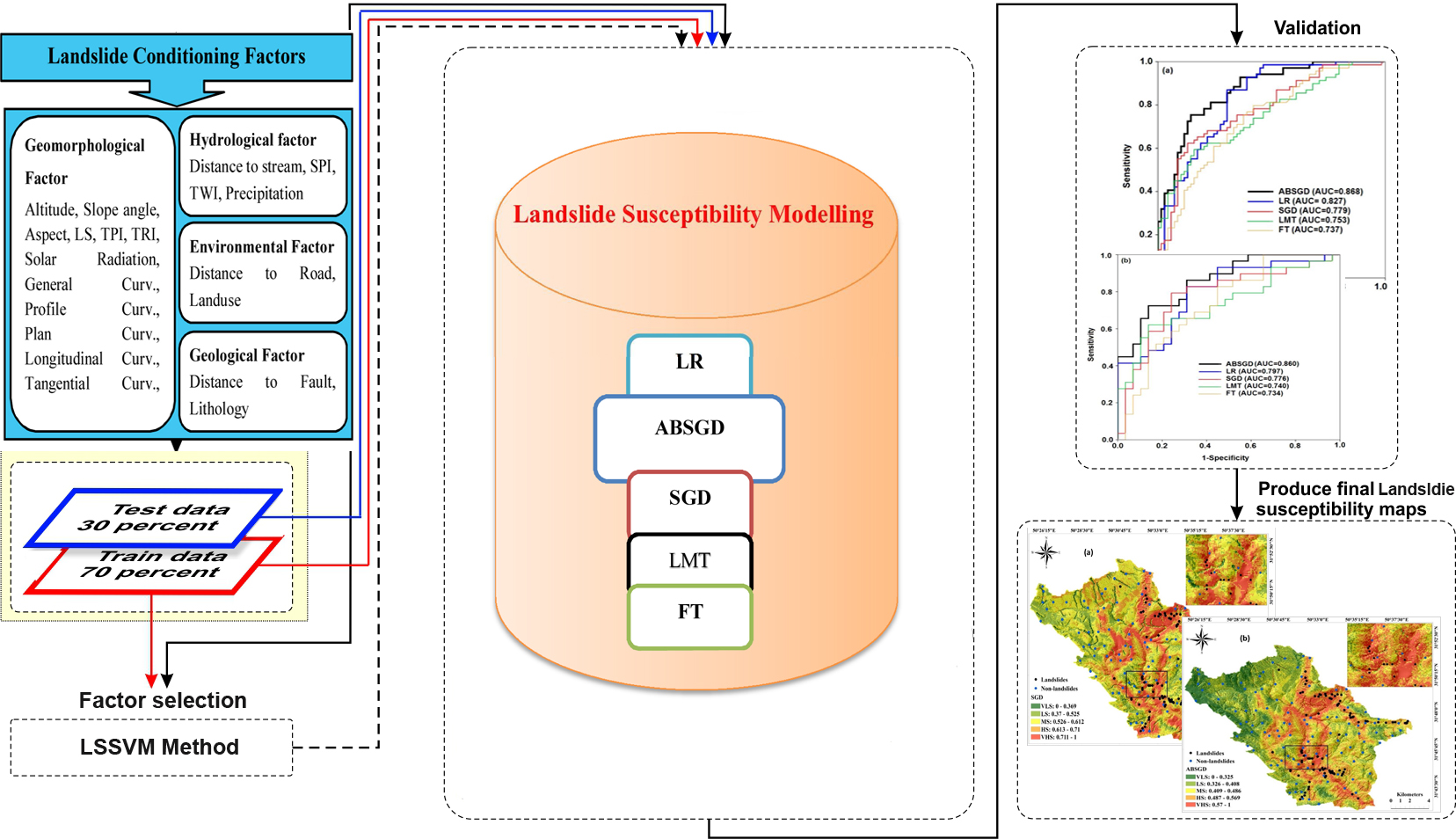
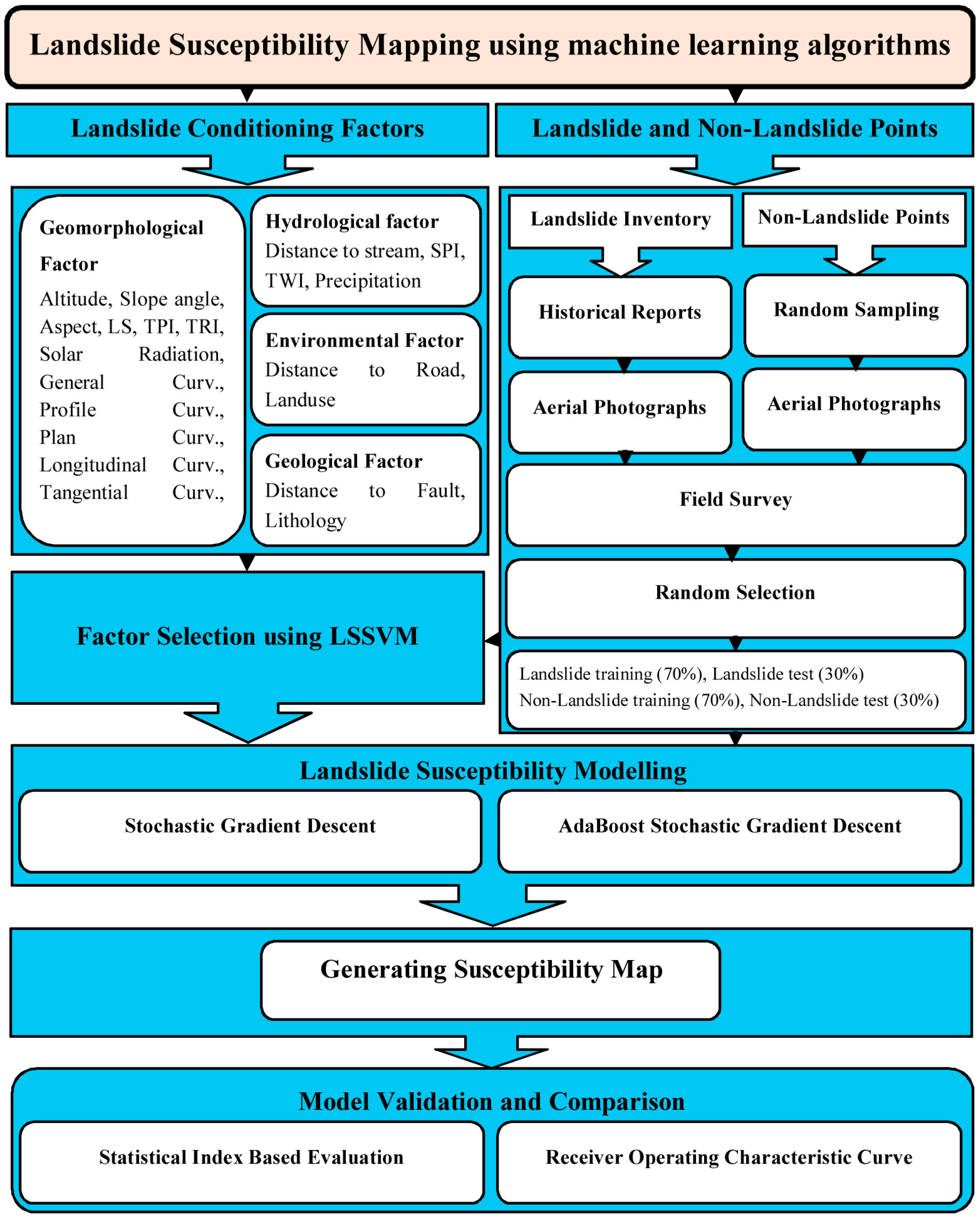
3. Methodology
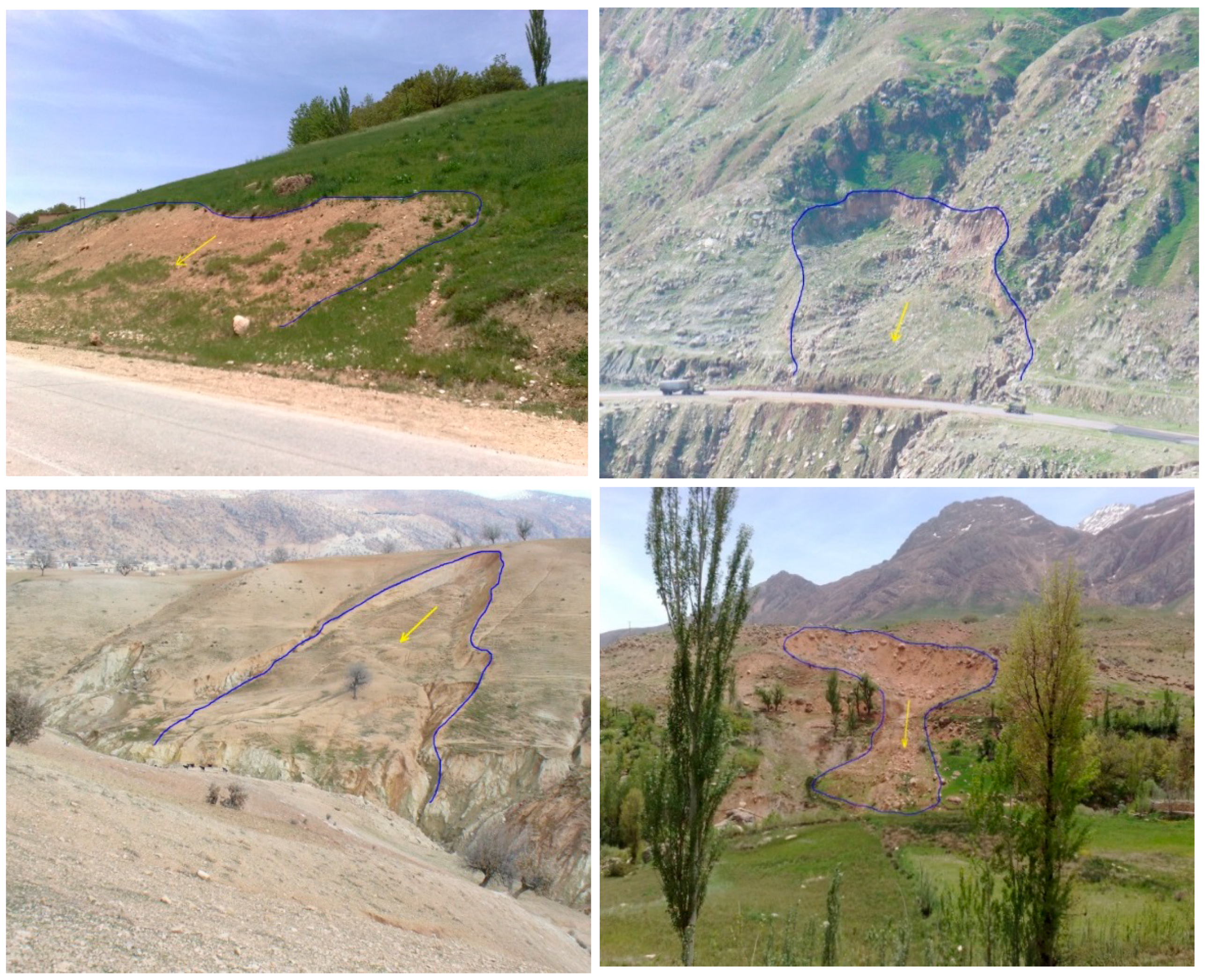
3.1. Landslide Inventory Map (LIM)
3.2. Landslide Conditioning Factors
3.3. AdaBoost Meta Classifier
3.4. Stochastic Gradient Descent Algorithm
3.5. Logistic Regression
3.6. Logistic Model Tree
3.7. Functional Tree
3.8. Factor Selection Using the Least Square Support Vector Machine (LSSVM)
3.9. Evaluation and Comparison of Algorithms
3.9.1. Statistical Index-Based Evaluation
3.9.2. AUC
4. Results and Analysis
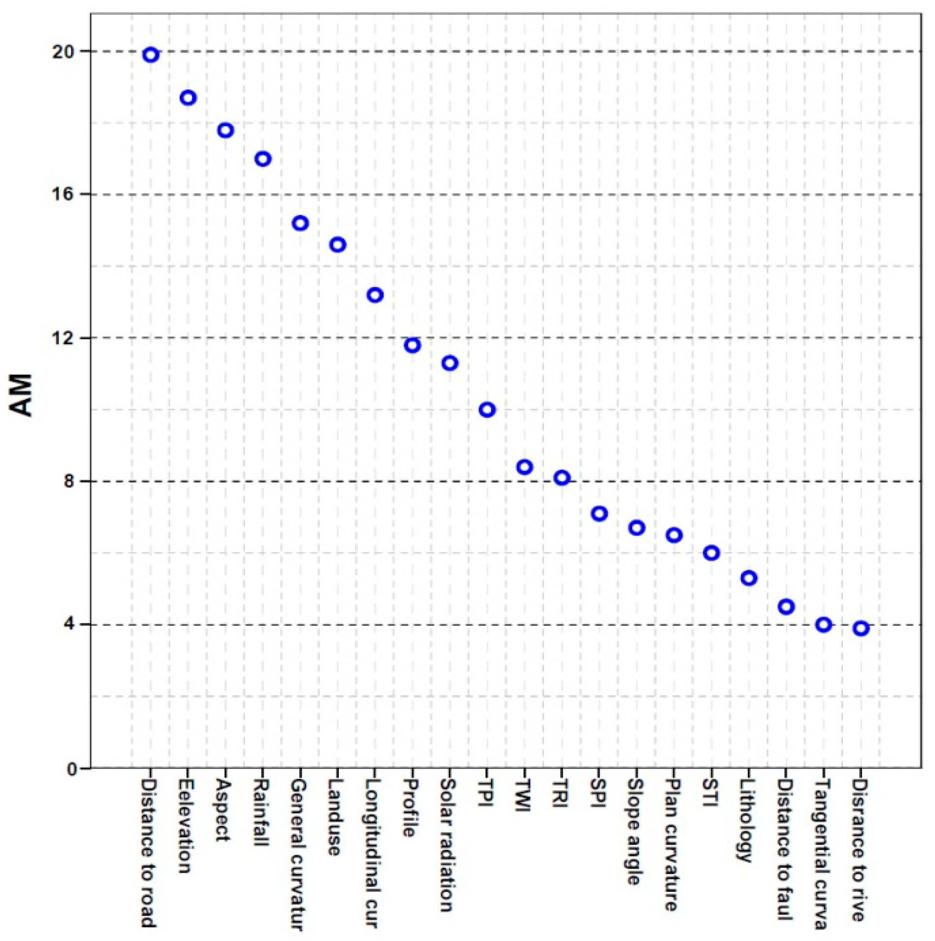
4.1. The Most Significant Conditioning Factors in the Modeling Process
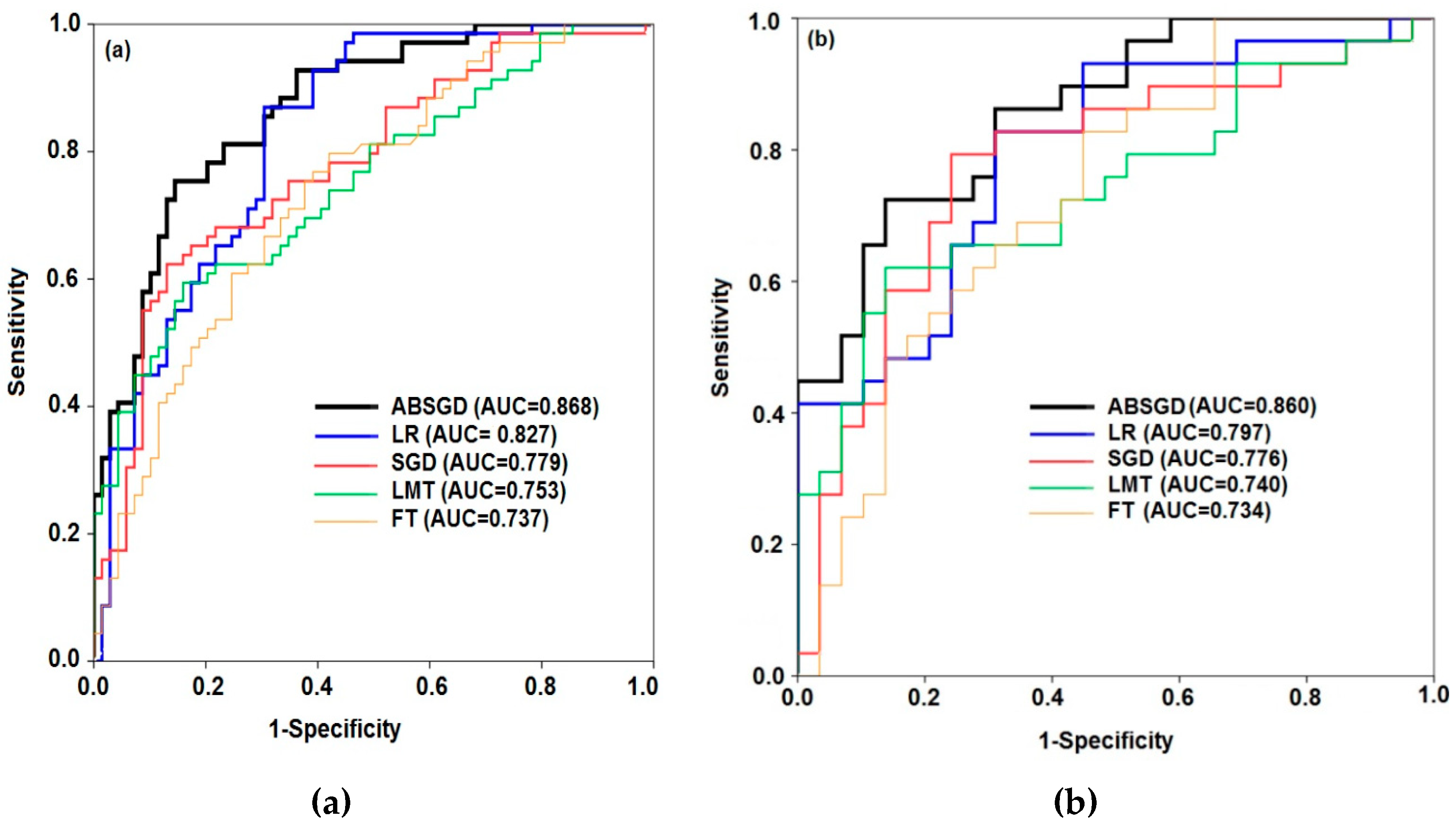
4.2. Model Validation and Comparison
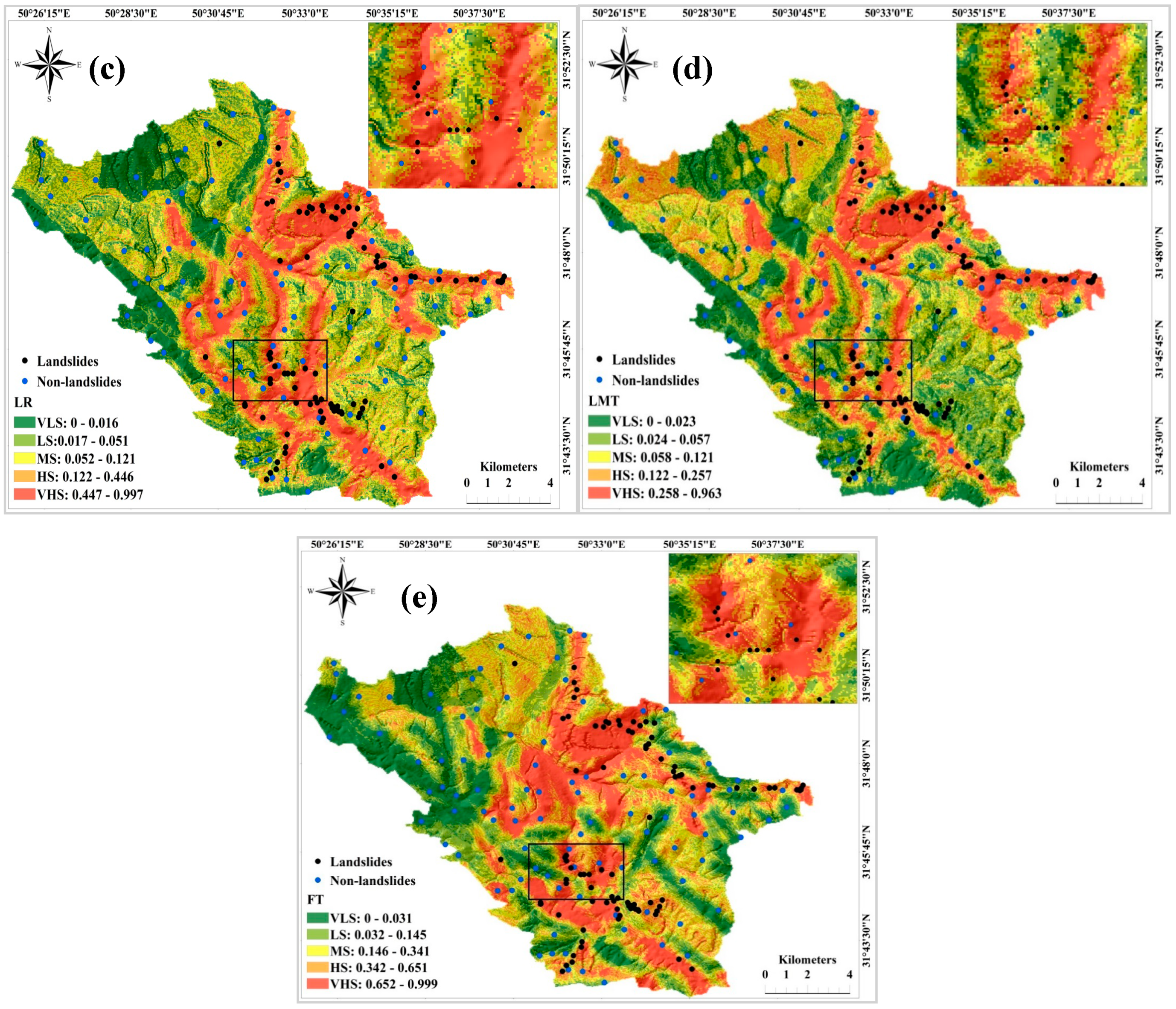
4.3. Landslide Susceptibility Mapping
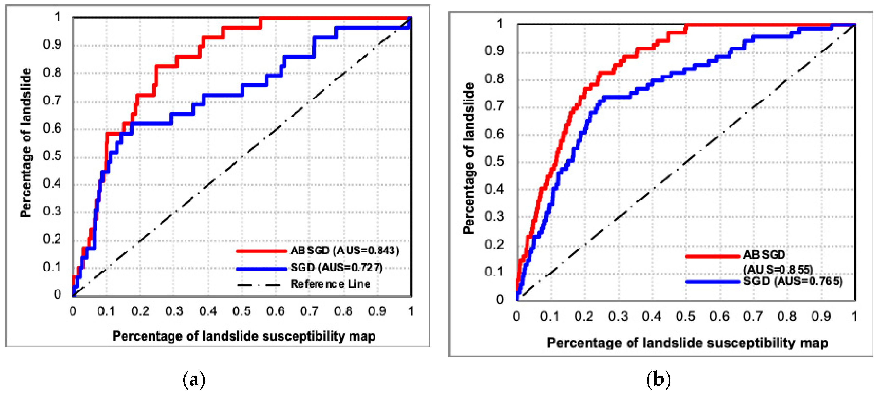
4.4. Map Verification and Comparison
5. Discussion
6. Conclusions
Author Contributions
Funding
Conflicts of Interest
References
- Dehnavi, A.; Aghdam, I.N.; Pradhan, B.; Varzandeh, M.H.M. A new hybrid model using step-wise weight assessment ratio analysis (swara) technique and adaptive neuro-fuzzy inference system (anfis) for regional landslide hazard assessment in iran. Catena 2015, 135, 122–148. [Google Scholar] [CrossRef]
- Petley, D. Global patterns of loss of life from landslides. Geology 2012, 40, 927–930. [Google Scholar] [CrossRef]
- Aleotti, P.; Chowdhury, R. Landslide hazard assessment: Summary review and new perspectives. Bull. Eng. Geol. Environ. 1999, 58, 21–44. [Google Scholar] [CrossRef]
- Sassa, K.; Canuti, P. Landslides-Disaster Risk Reduction; Springer Science & Business Media: Berlin/Heidelberg, Germany, 2008. [Google Scholar]
- Nadim, F.; Kjekstad, O.; Peduzzi, P.; Herold, C.; Jaedicke, C. Global landslide and avalanche hotspots. Landslides 2006, 3, 159–173. [Google Scholar] [CrossRef]
- Dowling, C.A.; Santi, P.M. Debris flows and their toll on human life: A global analysis of debris-flow fatalities from 1950 to 2011. Nat. Hazards 2014, 71, 203–227. [Google Scholar] [CrossRef]
- Chen, W.; Peng, J.; Hong, H.; Shahabi, H.; Pradhan, B.; Liu, J.; Zhu, A.-X.; Pei, X.; Duan, Z. Landslide susceptibility modelling using gis-based machine learning techniques for chongren county, jiangxi province, china. Sci. Total Environ. 2018, 626, 1121–1135. [Google Scholar] [CrossRef]
- Corominas, J.; van Westen, C.; Frattini, P.; Cascini, L.; Malet, J.-P.; Fotopoulou, S.; Catani, F.; Van Den Eeckhaut, M.; Mavrouli, O.; Agliardi, F. Recommendations for the quantitative analysis of landslide risk. Bull. Eng. Geol. Environ. 2014, 73, 209–263. [Google Scholar] [CrossRef]
- Shadman Roodposhti, M.; Aryal, J.; Shahabi, H.; Safarrad, T. Fuzzy shannon entropy: A hybrid gis-based landslide susceptibility mapping method. Entropy 2016, 18, 343. [Google Scholar] [CrossRef]
- Shafizadeh-Moghadam, H.; Minaei, M.; Shahabi, H.; Hagenauer, J. Big data in geohazard; pattern mining and large scale analysis of landslides in iran. Earth Sci. Inform. 2019, 12, 1–17. [Google Scholar] [CrossRef]
- Ercanoglu, M.; Gokceoglu, C. Use of fuzzy relations to produce landslide susceptibility map of a landslide prone area (west black sea region, turkey). Eng. Geol. 2004, 75, 229–250. [Google Scholar] [CrossRef]
- Zhao, C.; Lu, Z. Remote Sensing of Landslides—A Review; Multidisciplinary Digital Publishing Institute: Basel, Switzerland, 2018. [Google Scholar]
- Zhao, C.; Kang, Y.; Zhang, Q.; Lu, Z.; Li, B. Landslide identification and monitoring along the jinsha river catchment (wudongde reservoir area), china, using the insar method. Remote Sens. 2018, 10, 993. [Google Scholar] [CrossRef]
- Shahabi, H.; Hashim, M. Landslide susceptibility mapping using gis-based statistical models and remote sensing data in tropical environment. Sci. Rep. 2015, 5, 9899. [Google Scholar] [CrossRef]
- Golovko, D.; Roessner, S.; Behling, R.; Wetzel, H.-U.; Kleinschmit, B. Evaluation of remote-sensing-based landslide inventories for hazard assessment in southern kyrgyzstan. Remote Sens. 2017, 9, 943. [Google Scholar] [CrossRef]
- Kutlug Sahin, E.; Ipbuker, C.; Kavzoglu, T. Investigation of automatic feature weighting methods (fisher, chi-square and relief-f) for landslide susceptibility mapping. Geocarto Int. 2017, 32, 956–977. [Google Scholar] [CrossRef]
- Reichenbach, P.; Rossi, M.; Malamud, B.D.; Mihir, M.; Guzzetti, F. A review of statistically-based landslide susceptibility models. Earth-Sci. Rev. 2018, 180, 60–91. [Google Scholar] [CrossRef]
- Pradhan, B.; Seeni, M.I.; Kalantar, B. Performance evaluation and sensitivity analysis of expert-based, statistical, machine learning and hybrid models for producing landslide susceptibility maps. In Laser Scanning Applications in Landslide Assessment; Springer: Cham, Switzerland, 2017; pp. 193–232. [Google Scholar]
- Trigila, A.; Frattini, P.; Casagli, N.; Catani, F.; Crosta, G.; Esposito, C.; Iadanza, C.; Lagomarsino, D.; Mugnozza, G.S.; Segoni, S. Landslide susceptibility mapping at national scale: The italian case study. In Landslide Science and Practice; Springer: Berlin/Heidelberg, Germany, 2013; pp. 287–295. [Google Scholar]
- Kayastha, P.; Dhital, M.R.; De Smedt, F. Landslide susceptibility mapping using the weight of evidence method in the tinau watershed, nepal. Nat. Hazards 2012, 63, 479–498. [Google Scholar] [CrossRef]
- Tsangaratos, P.; Ilia, I.; Hong, H.; Chen, W.; Xu, C. Applying information theory and gis-based quantitative methods to produce landslide susceptibility maps in nancheng county, china. Landslides 2017, 14, 1091–1111. [Google Scholar] [CrossRef]
- Yalcin, A. Gis-based landslide susceptibility mapping using analytical hierarchy process and bivariate statistics in ardesen (turkey): Comparisons of results and confirmations. Catena 2008, 72, 1–12. [Google Scholar] [CrossRef]
- Park, S.; Choi, C.; Kim, B.; Kim, J. Landslide susceptibility mapping using frequency ratio, analytic hierarchy process, logistic regression and artificial neural network methods at the inje area, korea. Environ. Earth Sci. 2013, 68, 1443–1464. [Google Scholar] [CrossRef]
- Alizadeh, M.; Hashim, M.; Alizadeh, E.; Shahabi, H.; Karami, M.; Beiranvand Pour, A.; Pradhan, B.; Zabihi, H. Multi-criteria decision making (mcdm) model for seismic vulnerability assessment (sva) of urban residential buildings. ISPRS Int. J. Geo-Inf. 2018, 7, 444. [Google Scholar] [CrossRef]
- Choi, J.; Oh, H.-J.; Lee, H.-J.; Lee, C.; Lee, S. Combining landslide susceptibility maps obtained from frequency ratio, logistic regression and artificial neural network models using aster images and gis. Eng. Geol. 2012, 124, 12–23. [Google Scholar] [CrossRef]
- Regmi, A.D.; Devkota, K.C.; Yoshida, K.; Pradhan, B.; Pourghasemi, H.R.; Kumamoto, T.; Akgun, A. Application of frequency ratio, statistical index and weights-of-evidence models and their comparison in landslide susceptibility mapping in central nepal himalaya. Arabian J. Geosci. 2014, 7, 725–742. [Google Scholar] [CrossRef]
- Shirzadi, A.; Chapi, K.; Shahabi, H.; Solaimani, K.; Kavian, A.; Ahmad, B.B. Rock fall susceptibility assessment along a mountainous road: An evaluation of bivariate statistic, analytical hierarchy process and frequency ratio. Environ. Earth Sci. 2017, 76, 152. [Google Scholar] [CrossRef]
- Shahabi, H.; Ahmad, B.; Khezri, S. Evaluation and comparison of bivariate and multivariate statistical methods for landslide susceptibility mapping (case study: Zab basin). Arabian J. Geosci. 2013, 6, 3885–3907. [Google Scholar] [CrossRef]
- Chen, W.; Shahabi, H.; Shirzadi, A.; Hong, H.; Akgun, A.; Tian, Y.; Liu, J.; Zhu, A.-X.; Li, S. Novel hybrid artificial intelligence approach of bivariate statistical-methods-based kernel logistic regression classifier for landslide susceptibility modeling. Bull. Eng. Geol. Environ. 2018. [Google Scholar] [CrossRef]
- Akgun, A. A comparison of landslide susceptibility maps produced by logistic regression, multi-criteria decision and likelihood ratio methods: A case study at İzmir, turkey. Landslides 2012, 9, 93–106. [Google Scholar] [CrossRef]
- Pham, B.T.; Pradhan, B.; Bui, D.T.; Prakash, I.; Dholakia, M. A comparative study of different machine learning methods for landslide susceptibility assessment: A case study of uttarakhand area (india). Environ. Modell. Softw. 2016, 84, 240–250. [Google Scholar] [CrossRef]
- Michael, E.A.; Samanta, S. Landslide vulnerability mapping (lvm) using weighted linear combination (wlc) model through remote sensing and gis techniques. Mode. Earth Syst. Environ. 2016, 2, 88. [Google Scholar] [CrossRef]
- He, X.; Hong, Y.; Yu, X.; Cerato, A.B.; Zhang, X.; Komac, M. Landslides susceptibility mapping in oklahoma state using gis-based weighted linear combination method. In Landslide Science for a Safer Geoenvironment; Springer: Cham, Switzerland, 2014; pp. 371–377. [Google Scholar]
- Hong, H.; Shahabi, H.; Shirzadi, A.; Chen, W.; Chapi, K.; Ahmad, B.B.; Roodposhti, M.S.; Hesar, A.Y.; Tian, Y.; Bui, D.T. Landslide susceptibility assessment at the wuning area, china: A comparison between multi-criteria decision making, bivariate statistical and machine learning methods. Nat. Hazards 2018. [Google Scholar] [CrossRef]
- Conoscenti, C.; Ciaccio, M.; Caraballo-Arias, N.A.; Gómez-Gutiérrez, Á.; Rotigliano, E.; Agnesi, V. Assessment of susceptibility to earth-flow landslide using logistic regression and multivariate adaptive regression splines: A case of the belice river basin (western sicily, italy). Geomorphology 2015, 242, 49–64. [Google Scholar] [CrossRef]
- Chen, W.; Pourghasemi, H.R.; Naghibi, S.A. Prioritization of landslide conditioning factors and its spatial modeling in shangnan county, china using gis-based data mining algorithms. Bull. Eng. Geol. Environ. 2017. [Google Scholar] [CrossRef]
- Chen, W.; Pradhan, B.; Li, S.; Shahabi, H.; Rizeei, H.M.; Hou, E.; Wang, S. Novel hybrid integration approach of bagging-based fisher’s linear discriminant function for groundwater potential analysis. Nat. Resour. Res. 2019. [Google Scholar] [CrossRef]
- Azareh, A.; Rahmati, O.; Rafiei-Sardooi, E.; Sankey, J.B.; Lee, S.; Shahabi, H.; Ahmad, B.B. Modelling gully-erosion susceptibility in a semi-arid region, iran: Investigation of applicability of certainty factor and maximum entropy models. Sci. Total Environ. 2019, 655, 684–696. [Google Scholar] [CrossRef]
- Pradhan, B. Remote sensing and gis-based landslide hazard analysis and cross-validation using multivariate logistic regression model on three test areas in malaysia. Adv. Space Res. 2010, 45, 1244–1256. [Google Scholar] [CrossRef]
- Althuwaynee, O.F.; Pradhan, B.; Park, H.-J.; Lee, J.H. A novel ensemble bivariate statistical evidential belief function with knowledge-based analytical hierarchy process and multivariate statistical logistic regression for landslide susceptibility mapping. Catena 2014, 114, 21–36. [Google Scholar] [CrossRef]
- Chen, W.; Xie, X.; Peng, J.; Shahabi, H.; Hong, H.; Bui, D.T.; Duan, Z.; Li, S.; Zhu, A.-X. Gis-based landslide susceptibility evaluation using a novel hybrid integration approach of bivariate statistical based random forest method. Catena 2018, 164, 135–149. [Google Scholar] [CrossRef]
- Tien Bui, D.; Shahabi, H.; Shirzadi, A.; Chapi, K.; Alizadeh, M.; Chen, W.; Mohammadi, A.; Ahmad, B.; Panahi, M.; Hong, H. Landslide detection and susceptibility mapping by airsar data using support vector machine and index of entropy models in cameron highlands, malaysia. Remote Sens. 2018, 10, 1527. [Google Scholar] [CrossRef]
- Catani, F.; Lagomarsino, D.; Segoni, S.; Tofani, V. Landslide susceptibility estimation by random forests technique: Sensitivity and scaling issues. Nat. Hazards Earth Syst. Sci. 2013, 13, 2815–2831. [Google Scholar] [CrossRef]
- Guzzetti, F.; Reichenbach, P.; Ardizzone, F.; Cardinali, M.; Galli, M. Estimating the quality of landslide susceptibility models. Geomorphology 2006, 81, 166–184. [Google Scholar] [CrossRef]
- Jaafari, A.; Zenner, E.K.; Panahi, M.; Shahabi, H. Hybrid artificial intelligence models based on a neuro-fuzzy system and metaheuristic optimization algorithms for spatial prediction of wildfire probability. Agric. For. Meteorol. 2019, 266, 198–207. [Google Scholar] [CrossRef]
- Goetz, J.N.; Guthrie, R.H.; Brenning, A. Integrating physical and empirical landslide susceptibility models using generalized additive models. Geomorphology 2011, 129, 376–386. [Google Scholar] [CrossRef]
- Taheri, K.; Shahabi, H.; Chapi, K.; Shirzadi, A.; Gutiérrez, F.; Khosravi, K. Sinkhole susceptibility mapping: A comparison between bayes-based machine learning algorithms. Land Degrad. Dev. 2019. [Google Scholar] [CrossRef]
- Abedini, M.; Ghasemian, B.; Shirzadi, A.; Shahabi, H.; Chapi, K.; Pham, B.T.; Bin Ahmad, B.; Tien Bui, D. A novel hybrid approach of bayesian logistic regression and its ensembles for landslide susceptibility assessment. Geocarto Int. 2018. [Google Scholar] [CrossRef]
- Chen, W.; Shahabi, H.; Shirzadi, A.; Li, T.; Guo, C.; Hong, H.; Li, W.; Pan, D.; Hui, J.; Ma, M. A novel ensemble approach of bivariate statistical-based logistic model tree classifier for landslide susceptibility assessment. Geocarto Int. 2018. [Google Scholar] [CrossRef]
- Vahidnia, M.H.; Alesheikh, A.A.; Alimohammadi, A.; Hosseinali, F. A gis-based neuro-fuzzy procedure for integrating knowledge and data in landslide susceptibility mapping. Comput. Geosci. 2010, 36, 1101–1114. [Google Scholar] [CrossRef]
- Dickson, M.E.; Perry, G.L. Identifying the controls on coastal cliff landslides using machine-learning approaches. Environ. Modell. Softw. 2016, 76, 117–127. [Google Scholar] [CrossRef]
- Hong, H.; Liu, J.; Zhu, A.-X.; Shahabi, H.; Pham, B.T.; Chen, W.; Pradhan, B.; Bui, D.T. A novel hybrid integration model using support vector machines and random subspace for weather-triggered landslide susceptibility assessment in the wuning area (china). Environ. Earth Sci. 2017, 76, 652. [Google Scholar] [CrossRef]
- Pradhan, B. A comparative study on the predictive ability of the decision tree, support vector machine and neuro-fuzzy models in landslide susceptibility mapping using gis. Comput. Geosci. 2013, 51, 350–365. [Google Scholar] [CrossRef]
- Chen, W.; Zhang, S.; Li, R.; Shahabi, H. Performance evaluation of the gis-based data mining techniques of best-first decision tree, random forest and naïve bayes tree for landslide susceptibility modeling. Sci. Total Environ. 2018, 644, 1006–1018. [Google Scholar] [CrossRef]
- Bui, D.T.; Tuan, T.A.; Klempe, H.; Pradhan, B.; Revhaug, I. Spatial prediction models for shallow landslide hazards: A comparative assessment of the efficacy of support vector machines, artificial neural networks, kernel logistic regression and logistic model tree. Landslides 2016, 13, 361–378. [Google Scholar]
- Chen, W.; Pourghasemi, H.R.; Panahi, M.; Kornejady, A.; Wang, J.; Xie, X.; Cao, S. Spatial prediction of landslide susceptibility using an adaptive neuro-fuzzy inference system combined with frequency ratio, generalized additive model and support vector machine techniques. Geomorphology 2017, 297, 69–85. [Google Scholar] [CrossRef]
- Rahmati, O.; Naghibi, S.A.; Shahabi, H.; Bui, D.T.; Pradhan, B.; Azareh, A.; Rafiei-Sardooi, E.; Samani, A.N.; Melesse, A.M. Groundwater spring potential modelling: Comprising the capability and robustness of three different modeling approaches. J. Hydrol. 2018, 565, 248–261. [Google Scholar] [CrossRef]
- Ermini, L.; Catani, F.; Casagli, N. Artificial neural networks applied to landslide susceptibility assessment. Geomorphology 2005, 66, 327–343. [Google Scholar] [CrossRef]
- Bui, D.T.; Pradhan, B.; Lofman, O.; Revhaug, I.; Dick, O.B. Spatial prediction of landslide hazards in hoa binh province (vietnam): A comparative assessment of the efficacy of evidential belief functions and fuzzy logic models. Catena 2012, 96, 28–40. [Google Scholar]
- Tsai, F.; Lai, J.-S.; Chen, W.W.; Lin, T.-H. Analysis of topographic and vegetative factors with data mining for landslide verification. Ecol. Eng. 2013, 61, 669–677. [Google Scholar] [CrossRef]
- Pham, B.T.; Bui, D.; Prakash, I.; Dholakia, M. Evaluation of predictive ability of support vector machines and naive bayes trees methods for spatial prediction of landslides in uttarakhand state (india) using gis. J. Geomat. 2016, 10, 71–79. [Google Scholar]
- He, Q.; Shahabi, H.; Shirzadi, A.; Li, S.; Chen, W.; Wang, N.; Chai, H.; Bian, H.; Ma, J.; Chen, Y. Landslide spatial modelling using novel bivariate statistical based naïve bayes, rbf classifier and rbf network machine learning algorithms. Sci. Total Environ. 2019, 663, 1–15. [Google Scholar] [CrossRef]
- Zhang, T.; Han, L.; Chen, W.; Shahabi, H. Hybrid integration approach of entropy with logistic regression and support vector machine for landslide susceptibility modeling. Entropy 2018, 20, 884. [Google Scholar] [CrossRef]
- Tien Bui, D.; Shahabi, H.; Shirzadi, A.; Chapi, K.; Pradhan, B.; Chen, W.; Khosravi, K.; Panahi, M.; Bin Ahmad, B.; Saro, L. Land subsidence susceptibility mapping in south korea using machine learning algorithms. Sensors 2018, 18, 2464. [Google Scholar] [CrossRef]
- Pham, B.T.; Prakash, I.; Singh, S.K.; Shirzadi, A.; Shahabi, H.; Bui, D.T. Landslide susceptibility modeling using reduced error pruning trees and different ensemble techniques: Hybrid machine learning approaches. CATENA 2019, 175, 203–218. [Google Scholar] [CrossRef]
- Shirzadi, A.; Bui, D.T.; Pham, B.T.; Solaimani, K.; Chapi, K.; Kavian, A.; Shahabi, H.; Revhaug, I. Shallow landslide susceptibility assessment using a novel hybrid intelligence approach. Environ. Earth Sci. 2017, 76, 60. [Google Scholar] [CrossRef]
- Bui, D.T.; Pradhan, B.; Revhaug, I.; Nguyen, D.B.; Pham, H.V.; Bui, Q.N. A novel hybrid evidential belief function-based fuzzy logic model in spatial prediction of rainfall-induced shallow landslides in the lang son city area (vietnam). Geomat. Nat. Hazards Risk 2015, 6, 243–271. [Google Scholar] [CrossRef]
- He, S.; Pan, P.; Dai, L.; Wang, H.; Liu, J. Application of kernel-based fisher discriminant analysis to map landslide susceptibility in the qinggan river delta, three gorges, china. Geomorphology 2012, 171, 30–41. [Google Scholar] [CrossRef]
- Aghdam, I.N.; Varzandeh, M.H.M.; Pradhan, B. Landslide susceptibility mapping using an ensemble statistical index (wi) and adaptive neuro-fuzzy inference system (anfis) model at alborz mountains (iran). Environ. Earth Sci. 2016, 75, 1–20. [Google Scholar] [CrossRef]
- Chang, S.-H.; Wan, S. Discrete rough set analysis of two different soil-behavior-induced landslides in national shei-pa park, taiwan. Geosci. Front. 2015, 6, 807–816. [Google Scholar] [CrossRef]
- Nguyen, V.V.; Pham, B.T.; Vu, B.T.; Prakash, I.; Jha, S.; Shahabi, H.; Shirzadi, A.; Ba, D.N.; Kumar, R.; Chatterjee, J.M. Hybrid machine learning approaches for landslide susceptibility modeling. Forests 2019, 10, 157. [Google Scholar] [CrossRef]
- Chen, W.; Panahi, M.; Tsangaratos, P.; Shahabi, H.; Ilia, I.; Panahi, S.; Li, S.; Jaafari, A.; Ahmad, B.B. Applying population-based evolutionary algorithms and a neuro-fuzzy system for modeling landslide susceptibility. Catena 2019, 172, 212–231. [Google Scholar] [CrossRef]
- Jaafari, A.; Panahi, M.; Pham, B.T.; Shahabi, H.; Bui, D.T.; Rezaie, F.; Lee, S. Meta optimization of an adaptive neuro-fuzzy inference system with grey wolf optimizer and biogeography-based optimization algorithms for spatial prediction of landslide susceptibility. Catena 2019, 175, 430–445. [Google Scholar] [CrossRef]
- Berberian, M.; King, G. Towards a paleogeography and tectonic evolution of iran. Can. J. Earth Sci. 1981, 18, 210–265. [Google Scholar] [CrossRef]
- Azarnivand, H.; Alizadeh, E.; Sour, A.; Hajibeglo, A. The effects of range management plans of soil properties and rangelands vegetation (case study: Eshtehard rangelands). J. Rangel. Sci. 2012, 2, 625–633. [Google Scholar]
- Dhakal, A.S.; Amada, T.; Aniya, M. Landslide hazard mapping and its evaluation using gis: An investigation of sampling schemes for a grid-cell based quantitative method. Photogramm. Eng. Remote Sens. 2000, 66, 981–989. [Google Scholar]
- Congalton, R.G.; Green, K. Assessing the Accuracy of Remotely Sensed Data: Principles and Practices; CRC Press: Boca Raton, FL, USA, 2008. [Google Scholar]
- Neuhäuser, B.; Damm, B.; Terhorst, B. Gis-based assessment of landslide susceptibility on the base of the weights-of-evidence model. Landslides 2012, 9, 511–528. [Google Scholar] [CrossRef]
- Chen, W.; Shahabi, H.; Zhang, S.; Khosravi, K.; Shirzadi, A.; Chapi, K.; Pham, B.; Zhang, T.; Zhang, L.; Chai, H. Landslide susceptibility modeling based on gis and novel bagging-based kernel logistic regression. Appl. Sci. 2018, 8, 2540. [Google Scholar] [CrossRef]
- Tien Bui, D.; Shahabi, H.; Shirzadi, A.; Chapi, K.; Hoang, N.-D.; Pham, B.; Bui, Q.-T.; Tran, C.-T.; Panahi, M.; Bin Ahamd, B. A novel integrated approach of relevance vector machine optimized by imperialist competitive algorithm for spatial modeling of shallow landslides. Remote Sens. 2018, 10, 1538. [Google Scholar] [CrossRef]
- Freund, Y.; Schapire, R.E. A decision-theoretic generalization of on-line learning and an application to boosting. J. Comput. Syst. Sci. 1997, 55, 119–139. [Google Scholar] [CrossRef]
- Sun, J.; Jia, M.-Y.; Li, H. Adaboost ensemble for financial distress prediction: An empirical comparison with data from chinese listed companies. Expert Syst. Appl. 2011, 38, 9305–9312. [Google Scholar] [CrossRef]
- Wang, S.-J.; Mathew, A.; Chen, Y.; Xi, L.-F.; Ma, L.; Lee, J. Empirical analysis of support vector machine ensemble classifiers. Expert Syst. Appl. 2009, 36, 6466–6476. [Google Scholar] [CrossRef] [Green Version]
- West, D.; Dellana, S.; Qian, J. Neural network ensemble strategies for financial decision applications. Comput. Oper. Res. 2005, 32, 2543–2559. [Google Scholar] [CrossRef]
- Hong, H.; Liu, J.; Bui, D.T.; Pradhan, B.; Acharya, T.D.; Pham, B.T.; Zhu, A.-X.; Chen, W.; Ahmad, B.B. Landslide susceptibility mapping using j48 decision tree with adaboost, bagging and rotation forest ensembles in the guangchang area (china). Catena 2018, 163, 399–413. [Google Scholar] [CrossRef]
- Schwenk, H.; Bengio, Y. Boosting neural networks. Neural Comput. 2000, 12, 1869–1887. [Google Scholar] [CrossRef]
- Roe, B.P.; Yang, H.-J.; Zhu, J.; Liu, Y.; Stancu, I.; McGregor, G. Boosted decision trees as an alternative to artificial neural networks for particle identification. Nuclear Instrum. Methods Phys. Res. Sect. A 2005, 543, 577–584. [Google Scholar] [CrossRef] [Green Version]
- Bottou, L. Large-scale machine learning with stochastic gradient descent. In Proceedings of the 19th International Conference on Computational Statistics, Paris, France, 22–27 August 2010; pp. 177–186. [Google Scholar]
- Tsuruoka, Y.; Tsujii, J.I.; Ananiadou, S. Stochastic gradient descent training for l1-regularized log-linear models with cumulative penalty. In Proceedings of the Joint Conference of the 47th Annual Meeting of the ACL and the 4th International Joint Conference on Natural Language, Singapore, 2–7 August 2009; pp. 477–485. [Google Scholar]
- Gardner, W.A. Learning characteristics of stochastic-gradient-descent algorithms: A general study, analysis and critique. Signal Process. 1984, 6, 113–133. [Google Scholar] [CrossRef]
- Pham, B.T.; Tien Bui, D.; Prakash, I.; Nguyen, L.H.; Dholakia, M.B. A comparative study of sequential minimal optimization-based support vector machines, vote feature intervals and logistic regression in landslide susceptibility assessment using gis. Environ. Earth Sci. 2017, 76, 371. [Google Scholar] [CrossRef]
- Bai, S.-B.; Wang, J.; Lü, G.-N.; Zhou, P.-G.; Hou, S.-S.; Xu, S.-N. Gis-based logistic regression for landslide susceptibility mapping of the zhongxian segment in the three gorges area, china. Geomorphology 2010, 115, 23–31. [Google Scholar] [CrossRef]
- Lee, S.; Pradhan, B. Landslide hazard mapping at selangor, malaysia using frequency ratio and logistic regression models. Landslides 2007, 4, 33–41. [Google Scholar] [CrossRef]
- Landwehr, N.; Hall, M.; Frank, E. Logistic model trees. Mach. Learn. 2005, 59, 161–205. [Google Scholar] [CrossRef]
- Chen, W.; Xie, X.; Wang, J.; Pradhan, B.; Hong, H.; Bui, D.T.; Duan, Z.; Ma, J. A comparative study of logistic model tree, random forest and classification and regression tree models for spatial prediction of landslide susceptibility. Catena 2017, 151, 147–160. [Google Scholar] [CrossRef]
- Pham, B.T.; Tien Bui, D.; Pourghasemi, H.R.; Indra, P.; Dholakia, M.B. Landslide susceptibility assesssment in the uttarakhand area (india) using gis: A comparison study of prediction capability of naïve bayes, multilayer perceptron neural networks and functional trees methods. Theor. Appl. Climatol. 2015, 122, 1–19. [Google Scholar] [CrossRef]
- Suykens, J.A.; De Brabanter, J.; Lukas, L.; Vandewalle, J. Weighted least squares support vector machines: Robustness and sparse approximation. Neurocomputing 2002, 48, 85–105. [Google Scholar] [CrossRef]
- Suykens, J.A.; Vandewalle, J. Least squares support vector machine classifiers. Neural Process. Lett. 1999, 9, 293–300. [Google Scholar] [CrossRef]
- Smola, A.J.; Schölkopf, B.; Müller, K.-R. The connection between regularization operators and support vector kernels. Neural Netw. 1998, 11, 637–649. [Google Scholar] [CrossRef] [Green Version]
- Beguería, S. Validation and evaluation of predictive models in hazard assessment and risk management. Nat. Hazards 2006, 37, 315–329. [Google Scholar] [CrossRef]
- Pham, B.T.; Nguyen, V.-T.; Ngo, V.-L.; Trinh, P.T.; Ngo, H.T.T.; Bui, D.T. A novel hybrid model of rotation forest based functional trees for landslide susceptibility mapping: A case study at kon tum province, vietnam. In Proceedings of the International Conference on Geo-Spatial Technologies and Earth Resources, Hanoi, Vietnam, 5–6 October 2017; pp. 186–201. [Google Scholar]
- Pham, B.T.; Prakash, I.; Bui, D.T. Spatial prediction of landslides using a hybrid machine learning approach based on random subspace and classification and regression trees. Geomorphology 2018, 303, 256–270. [Google Scholar] [CrossRef]
- Shirzadi, A.; Solaimani, K.; Roshan, M.H.; Kavian, A.; Chapi, K.; Shahabi, H.; Keesstra, S.; Ahmad, B.B.; Bui, D.T. Uncertainties of prediction accuracy in shallow landslide modeling: Sample size and raster resolution. Catena 2019, 178, 172–188. [Google Scholar] [CrossRef]
- Bui, D.T.; Ho, T.-C.; Pradhan, B.; Pham, B.-T.; Nhu, V.-H.; Revhaug, I. Gis-based modeling of rainfall-induced landslides using data mining-based functional trees classifier with adaboost, bagging and multiboost ensemble frameworks. Environ. Earth Sci. 2016, 75, 1101. [Google Scholar]
- Gorsevski, P.V.; Gessler, P.E.; Foltz, R.B.; Elliot, W.J. Spatial prediction of landslide hazard using logistic regression and roc analysis. Trans. GIS 2006, 10, 395–415. [Google Scholar] [CrossRef]
- Shafizadeh-Moghadam, H.; Valavi, R.; Shahabi, H.; Chapi, K.; Shirzadi, A. Novel forecasting approaches using combination of machine learning and statistical models for flood susceptibility mapping. J. Environ. Manag. 2018, 217, 1–11. [Google Scholar] [CrossRef]
- Khosravi, K.; Pham, B.T.; Chapi, K.; Shirzadi, A.; Shahabi, H.; Revhaug, I.; Prakash, I.; Bui, D.T. A comparative assessment of decision trees algorithms for flash flood susceptibility modeling at haraz watershed, northern iran. Sci. Total Environ. 2018, 627, 744–755. [Google Scholar] [CrossRef]
- Bui, D.T.; Ho, T.C.; Revhaug, I.; Pradhan, B.; Nguyen, D.B. Landslide susceptibility mapping along the national road 32 of vietnam using gis-based j48 decision tree classifier and its ensembles. In Cartography from Pole to Pole; Springer: Berlin/Heidelberg, Germany, 2014; pp. 303–317. [Google Scholar]
- Li, X.; Wang, L.; Sung, E. Adaboost with svm-based component classifiers. Eng. Appl. Artif. Intell. 2008, 21, 785–795. [Google Scholar] [CrossRef]
- Viola, P.; Jones, M. Robust Real-Time Face Detection; IEEE: Piscataway Township, NJ, USA, 2001; p. 747. [Google Scholar]


| Factors | Classes | GIS Data Type | Scale | Classification Method |
|---|---|---|---|---|
| Land use | (1) Dry farming; (2) Sparse forest; (3) Dense forest; (4) Poor rangeland; (5) Good rangeland; (6) Residential area; (7) Rock outcrop | Polygon | 1:25,000 | Supervised classification |
| Lithology * | (1) Mmm; (2) MPlsma; (3) PlCb; (4) Qal; (5) Q2t; (6) Q3t; (7) Edj; (8) Klt; (9) Kmg; (10) KlSi | Polygon | 1: 100,000 | Lithological classification |
| Average annual precipitation (mm) | (1) 523–650; (2) 650–800 (3) 800–950; (4) 950–1100; (5) 1100–1250; (6) 1250< | GRID | 10 m × 10 m | Natural breaks |
| Altitude (m) | (1) 1370–1620; (2) 1620–1870; (3) 1870–2120; (4) 2120–2370; (5) 2370–2620; (6) 2620–2870; (7) 2870–3120; (8) 3120–3375 | GRID | 10 m × 10 m | Natural breaks |
| Slope angle (˚) | (1) 0–5; (2) 5–10; (3) 10–15; (4) 15–20; (5) 20–30; (6) 30–45; (7) 45< | GRID | 10 m × 10 m | Manual |
| Aspect (˚) | (1) −1–0; (2) 0–22.5, 337.5–360; (3) 22.5–67.5; (4) 67.5–112.5; (5) 112.5–157.5; (6) 157.5–202.5; (7) 202.5–247.5; (8) 247.5–292.5; (9) 292.5–337.5 | GRID | 10 m × 10 m | Azimuth classification |
| LS | (1) <−70: (2) −70–−45; (3) −45–−15; (4) −15–15; (5) 15–45; (6) 45< | GRID | 10 m × 10 m | Natural breaks |
| General curvature | (1) <−0.1; (2) −0.1–−0.05; (3) −0.05–0; (4) 0–0.05; (5) 0.05< | GRID | 10 m × 10 m | Natural breaks |
| Profile curvature | (1) −1.369- −0.084; (2) −0.084–−0.008; (3) −0.008–0.26 | GRID | 10 m × 10 m | Natural breaks |
| Plan curvature | (1) −49.714–−0.0119; (2) −0.0119–0.0008; (3) 0.0008–0.0143; (4) 0.0143–8.3923 | GRID | 10 m × 10 m | Natural breaks |
| Longitudinal curvature | (1) <−0.1; (2) −0.1–−0.05; (3) −0.05–0; (4) 0–0.05; (5) 0.05–1; (6) 0.1–1.37 | GRID | 10 m × 10 m | Natural breaks |
| Tangential curvature | (1) −1.21–−0.051; (2) −1.21–−0.004; (3) −0.004–0.28 | GRID | 10 m × 10 m | Natural breaks |
| Solar radiation | (1) <350,000; (2) 350,000–700,000 (3) 700,000–1,050,000; (4) 1,050,000–1,400,000; (5) 1,400,000–1,750,000; (6) 1,750,000< | GRID | 10 m × 10 m | Natural breaks |
| SPI | (1) 4–6; (2) 6–8; (3) 8–10; (4) 10–12; (5) 12–14; (6) 14–16; (7) 16–18; (8) 18–20 | GRID | 10 m × 10 m | Natural breaks |
| TPI | (1) <−30; (2) −30–−15; (3) −15–0; (4) 0–15; (5) 15–30; (6) 30< | GRID | 10 m × 10 m | Natural breaks |
| TWI | (1) 4.71–6.69; (2) 6.69–8.67; (3) 8.67–10.56; (4) 10.56–12.64; (5) 12.64–14.62; (6) 14.62–16.60; (7) 16.60–18.58; (8) 18.58–20.56 | GRID | 10 m × 10 m | Natural breaks |
| TRI | (1) <5; (2) 5–15; (3) 15–25; (4) 25–35; (5) 35–45; (6) 45< | GRID | 10 m × 10 m | Natural breaks |
| Distance to stream (m) | (1) 0–100; (2) 100–200; (3)200–300; (4) 300–400; (5) 400–500, (6) 500< | Line | 1:25,000 | Manual |
| Distance to road (m) | (1) 0–100; (2) 100–200; (3)200–300; (4) 300–400; (5) 400–500, (6) 500< | Line | 1:25,000 | Manual |
| Distance to fault (m) | (1) 0–100; (2) 100–200; (3)200–300; (4) 300–400; (5) 400–500, (6) 500< | Line | 1: 100,000 | Manual |
| Predicted class | Actual class | ||
| Landslide (1) | Non-landslide (0) | ||
| Landslide (1) | TP | FP | |
| Non-landslide (0) | FN | TN | |
| ABSGD | SGD | LR | LMT | FT | |||||||
|---|---|---|---|---|---|---|---|---|---|---|---|
| T | V | T | V | T | V | T | V | T | V | ||
| TP | 61 | 20 | 56 | 19 | 58 | 21 | 54 | 18 | 52 | 18 | |
| TN | 57 | 25 | 58 | 23 | 60 | 22 | 59 | 25 | 59 | 21 | |
| FP | 8 | 9 | 13 | 10 | 11 | 8 | 12 | 12 | 10 | 11 | |
| FN | 12 | 4 | 11 | 6 | 9 | 7 | 15 | 4 | 17 | 8 | |
| SST | 0.836 | 0.833 | 0.836 | 0.760 | 0.866 | 0.750 | 0.783 | 0.818 | 0.754 | 0.692 | |
| SPC | 0.877 | 0.735 | 0.817 | 0.697 | 0.845 | 0.733 | 0.831 | 0.676 | 0.855 | 0.656 | |
| ACC | 0.855 | 0.776 | 0.826 | 0.724 | 0.855 | 0.741 | 0.807 | 0.729 | 0.804 | 0.672 | |
| RMSE | 0.323 | 0.411 | 0.446 | 0.531 | 0.338 | 0.443 | 0.451 | 0.536 | 0.502 | 0.540 | |
| AUC | 0.941 | 0.861 | 0.904 | 0.830 | 0.917 | 0.839 | 0.871 | 0.731 | 0.819 | 0.708 | |
| Algorithm | Parameters |
|---|---|
| SGD | Bach size, 100; Debug, False; Do not check capability, False; Not normalized, true; Do not replace missing, False; Epoch, 500; Epsilon, 0.001; Lambda, 0.0001; Learning rate, 0.01, Loss function, Logistic regression; Number of decimal places, 2; Number of seeds, 1. |
| ABSGD | Batch size, 100; Classifier, SGD; Debug, False; Do not check capability, False; Number of decimal places, 2; Number of iterations, 10; Number of seeds, 1; Use resampling, False; Weight threshold, 100. |
© 2019 by the authors. Licensee MDPI, Basel, Switzerland. This article is an open access article distributed under the terms and conditions of the Creative Commons Attribution (CC BY) license (http://creativecommons.org/licenses/by/4.0/).
Share and Cite
Tien Bui, D.; Shahabi, H.; Omidvar, E.; Shirzadi, A.; Geertsema, M.; Clague, J.J.; Khosravi, K.; Pradhan, B.; Pham, B.T.; Chapi, K.; et al. Shallow Landslide Prediction Using a Novel Hybrid Functional Machine Learning Algorithm. Remote Sens. 2019, 11, 931. https://0-doi-org.brum.beds.ac.uk/10.3390/rs11080931
Tien Bui D, Shahabi H, Omidvar E, Shirzadi A, Geertsema M, Clague JJ, Khosravi K, Pradhan B, Pham BT, Chapi K, et al. Shallow Landslide Prediction Using a Novel Hybrid Functional Machine Learning Algorithm. Remote Sensing. 2019; 11(8):931. https://0-doi-org.brum.beds.ac.uk/10.3390/rs11080931
Chicago/Turabian StyleTien Bui, Dieu, Himan Shahabi, Ebrahim Omidvar, Ataollah Shirzadi, Marten Geertsema, John J. Clague, Khabat Khosravi, Biswajeet Pradhan, Binh Thai Pham, Kamran Chapi, and et al. 2019. "Shallow Landslide Prediction Using a Novel Hybrid Functional Machine Learning Algorithm" Remote Sensing 11, no. 8: 931. https://0-doi-org.brum.beds.ac.uk/10.3390/rs11080931