Article

Determination of Bathing Water Quality Using Thermal Images Landsat 8 on the West Coast of Tangier: Preliminary Results

by
El Khalil Cherif
1,*,
Farida Salmoun
1 and
Francisco Javier Mesas-Carrascosa
2
1
Laboratory of Physical Chemistry of Materials, Natural Substances and Environment, Sciences and Technology Faculty, Abdelmalek Essaadi University, Tangier 90090, Morocco
2
Department of Graphic Engineering and Geomatics, University of Cordoba, Campus de Rabanales, 14071 Córdoba, Spain
*
Author to whom correspondence should be addressed.
Submission received: 22 March 2019 / Revised: 18 April 2019 / Accepted: 18 April 2019 / Published: 23 April 2019

Abstract

:
Bathing water quality has been monitored in the west coast of Tangier, Morocco due to increased urban and industrial discharge through the Boukhalef river, using in-situ bacteriological measurements which demand high economical and temporal costs. In this study, Landsat 8 Thermal Infrared Sensor (TIRS) images were used as an alternative to the classical method, for determining bathing water quality to help decision makers obtain up-to-date and cost-effective information for coastal environment protection. For this purpose, during spring and summer 2017, seven sampling points were examined in terms of bacteriological parameters: Total Coliforms (TC), Faecal Coliforms (FC), Intestinal Enterococci (IE) and Escherichia coli (E. coli). Also, a spatial-temporal analysis was performed in this temporal window to detect temperature anomalies and their spatial distribution along the coastal bathing area. In addition, a relationship between in-situ bacteriological parameter measurements and temperature from satellite images was analyzed. The results of the water temperature distribution showed the highest values next to the Boukhalef river mouth, as well as the poorest water quality according to in-situ measurements, while lower values and better water quality status were observed moving away from the Boukhalef river mouth. The relationship between water temperature and bacterial concentration showed a high correlation coefficient (R2 = 0.85). Consequently, the model development approaches used may be useful in estimating bacterial concentration in coastal bathing areas and can serve to create a monitoring system to support decision makers in the protection actions of the coast.

Graphical Abstract

1. Introduction

Over 40% of the world’s population lives alongside the coastal zone [1]. Coastal waters offer some of the best landscape areas used for recreational activities [2] and for other important purposes; marine aquaculture, commercial navigation or as a repository for sewage and industrial waste [3]. Such activities are not always compatible with one another. Moreover, their increase can cause changes to this ecosystem and can endanger human health and the habitats of aquatic organisms [4,5]. Therefore, sustainable coastal water requires water resource control and continuous monitoring. In addition, water treatment requires an understanding of the quality of water bodies.
Water quality takes into account the thermal, physical, chemical, and biological characteristics of a body of water. It is used as an index to determine the water’s suitability for human consumption or recreational use. Defining water quality can be difficult, as its usage varies widely: For example, parameters of water that are suitable for crop irrigation differ from those for human consumption. Furthermore, it is usually linked to water consumer safety. There is a wide range of both chemical and microbial contaminants that may be found in drinking water, some of which can have negative health effects on consumers. Understanding the nature of sources of pollutants and how these may enter the water supply is important for assuring water safety.
In this context, water quality has a direct relation to urban, agricultural and industrial discharges. Furthermore, urban waste waters cause fecal pollution of surface water which is a worldwide concern. In addition, urban storm water runoff, containing large quantities of fecal microbes, has been shown to contribute to surface water quality [6]. It has an important effect on both public health and the economy as a result of beach closures, limited fishing or degradation of drinking water sources [7]. On the other hand, agricultural run-off and industrial waste water contribute to eutrophication processes causing an accumulation of phytoplankton. The nutrient increment supports the excessive growth of plants that causes the water to become more turbid, affects fish populations or accelerates algae blooms [8]. Therefore, the quality of water affects all components of the aquatic ecosystem [9]
Key water quality indicators would include dissolved oxygen, water temperature, pH, Escherichia coli (E. coli), specific conductance, nitrates, transparency and the visual test [10]. These water quality indicators, including physical, chemical and biological properties, are traditionally determined by in-situ measurements and collected samples to be analyzed in the laboratory [11], and are compared with their standard value to determine water body status [12]. Moreover, several water quality indexes have been developed by translating these water quality indicators into numerical scores [13]. Effective assessment of water consumer safety is based on probabilistic data, expert opinions and linguistic descriptions; in addition, it is also associated with subjective factors [14]. Therefore, new methods, such as neural networks, are needed to manage water consumer safety [15]. Although, the classical method of determining these water quality indicators offers valuable information it requires high economical and temporal costs [16] and it is not feasible to obtain these water quality parameters regularly on a regional scale [17].
With advances in Earth observation programs, remote sensing techniques have become useful tools for monitoring and evaluating water quality in a more efficient manner, being in use since the 1970s [18,19]. Most of the studies using remote sensing techniques have focused on optical properties as well as chlorophyll [20,21], total suspended matters [22], turbidity [23] and dissolved organic matters [24,25]. These studies were performed using different sensors onboard satellites or aircraft platforms with different spatial and spectral resolutions, being necessary to understand their properties to choose the most adequate for the objectives of the study [11].
Water temperature surface is an important parameter for biological, chemical and physical processes occurring within water. Moreover, air and water temperature interaction is important because it regulates these processes. Changes in water temperature have an important environmental impact [26]. Therefore, mapping and monitoring coastal waters is necessary to protect the health of the coastal marine ecosystem and to ensure bathers’ health. Sea Surface Temperature (SST) is an important factor that represents gradient in the first several centimeters of the water, which is usually sustained by the atmospheric heat flux [27]. Traditional shipboard SST measurements provide accurate temperature values, however they are time-consuming and expensive [16]. On the other hand, thermal images from satellite or aircraft platforms provide a regular sampling of SST, improving measurement capability [27,28]. SST measurements from thermal bands have been used to study the impact of nuclear power plants in the coastal ecosystem [29], its relationship with earthquakes [30], to monitor thermal stress in marine ecosystems [31,32], turbidity [33] or to detect groundwater discharge areas [34] or oil spills [35].
Coastal water quality is often monitored through bacteriological analyses [4,36,37]. Generally, the control of coastal waters quality is carried out measuring the concentration of Escherichia Coli, Intestinal Enterococci, Total Coliforms, Faecal Coliforms [38]. These parameters indicate the quality of the coastal waters and assess the environmental problems [39]. It has been demonstrated that Escherichia coli is commonly used as a good indicator of fecal contamination in rivers and coastal waters [40,41]. However, since most coastal zones stretch for thousands of kilometers, it is not an easy task to identify the coastal reaches that require early and increased attention. In this context, remote sensing emerges as a potentially important source of information for the detection of marine pollution [42,43,44,45].
Fecal bacteria models have been attempted in limited applications [46], for example in beach recreation areas [47], storm water ponds [48] and shellfish management settings [49]. These models use different predictors, including in-situ water temperature measurements. The survival of fecal micro-organisms in water may be significantly influenced by the combination of high temperature, low conductivity and low pH [50]. Focused on fecal pollutants, remotely sensed images have been used mainly to determine land covers in stream watersheds [51,52,53]. Showing that water quality indicators, temperature and fecal pollutants, are related.
In the present study, fecal bacteria were measured in bathing waters and their association with SST measurements was tested from remotely sensed thermal images in the west coast of Tangier, Morocco. This study focused first on analyzing spatio-temporal variation of bacteriological pollutant and SST, and second on building a statistical model based on SST values from remotely sensed images to predict bacteria concentrations in bathing waters.

2. Material and methods

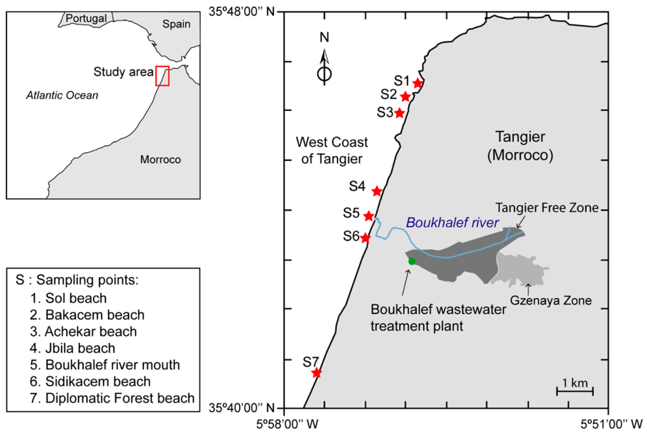
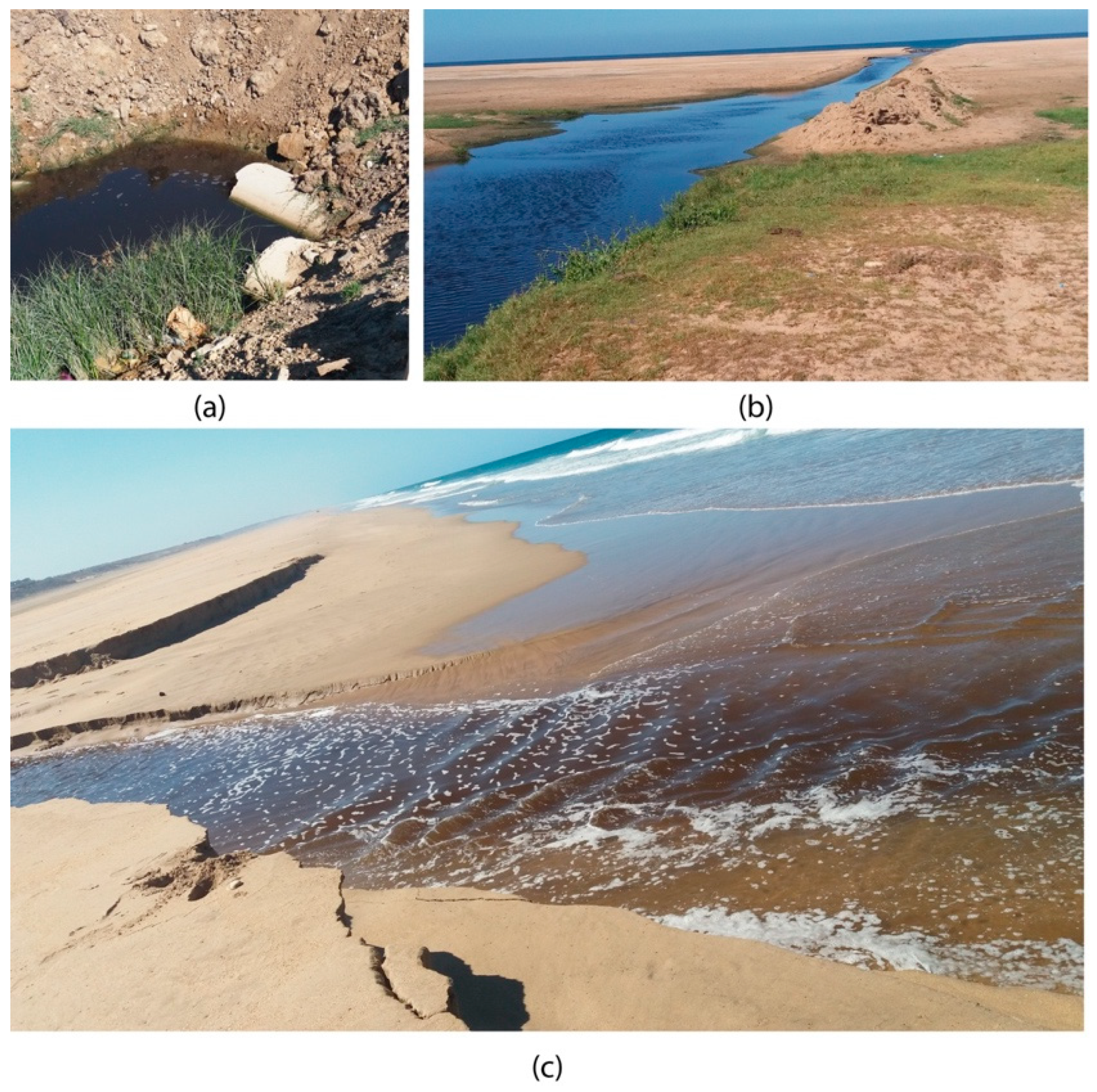
2.1. Site Description

The study area is located in north-western Morocco (Figure 1), (upper left 35°46′38″N, 5°57′53″W; lower right 35°40′32″N, 5°55′38″W, coordinate reference system WGS-84) and occupies a coastal stretch of 15 km, along the west coast of Tangier, covering six beaches from Sol beach to the Diplomatic Forest beach, including the Boukhalef watershed. The west coast of Tangier is one of the most important popular tourist destinations on the Atlantic coast [54]. There are numerous human activities in the area including industries, urban areas and a series of seaside resorts and hotels along the coastline that have a negative impact on the Boukhalef river [55]. Figure 2 represents a point of pollutant discharge into the Boukhalef river (Figure 2a), following its stream (Figure 2b) until the coast is reached (Figure 2c) at the river mouth (Figure 1, S5). The waste waters of these activities are often characterized by a high concentration of pollution parameters [56]. Therefore, the absence or weakness of treatment of this industrial drainage leads to potential hazards. However, close to the Boukhalef river mouth there is a wastewater treatment station and two industrial zones, as well as areas with touristic and urban activities. In addition, the distribution of discharges from the Boukhalef river is under the effect of the wind, coastal currents and rain conditions, meaning that the western coast of Morocco is characterized by strong hydrodynamic conditions. Moreover, two coastal beaches, Jbila (Figure 1, S4) and Sidikacem (Figure 1, S6), are known to be chronically contaminated due to large volumes of industrial liquid discharge from the Boukhalef river. These two beaches are at a distance of 800 m from S5.
To complete this study, four beaches at different distances to point S5 have been included to map out the area of influence from the river mouth. To the north, the following beaches have been taken into account: Sol (S1, 5300 m), Bacacem (S2, 4600 m) and Achekar (S3, 4000 m), while in the southern part, the Diplomatic Forest has been considered (S7, 6100 m).

2.2. Landsat Imagery

A total of four Landsat 8 images covering the west coast of Tangier have been used in this study, from April–August 2017 (Table 1). The month of July has not been included in the study because we did not have a cloud-free image for that period of time. Landsat 8 carries two sensors; the Operational Land Imager (OLI) and the Thermal Infrared Sensor (TIRS). OLI collects data in nine spectral bands with a spatial resolution of 30 m (15 m for panchromatic band 8) [57]. TIRS measures thermal data at 100 m spatial resolution using two bands at 10 and 12 μm [58]. In this study, we used standard terrain corrected data, level 1 T.

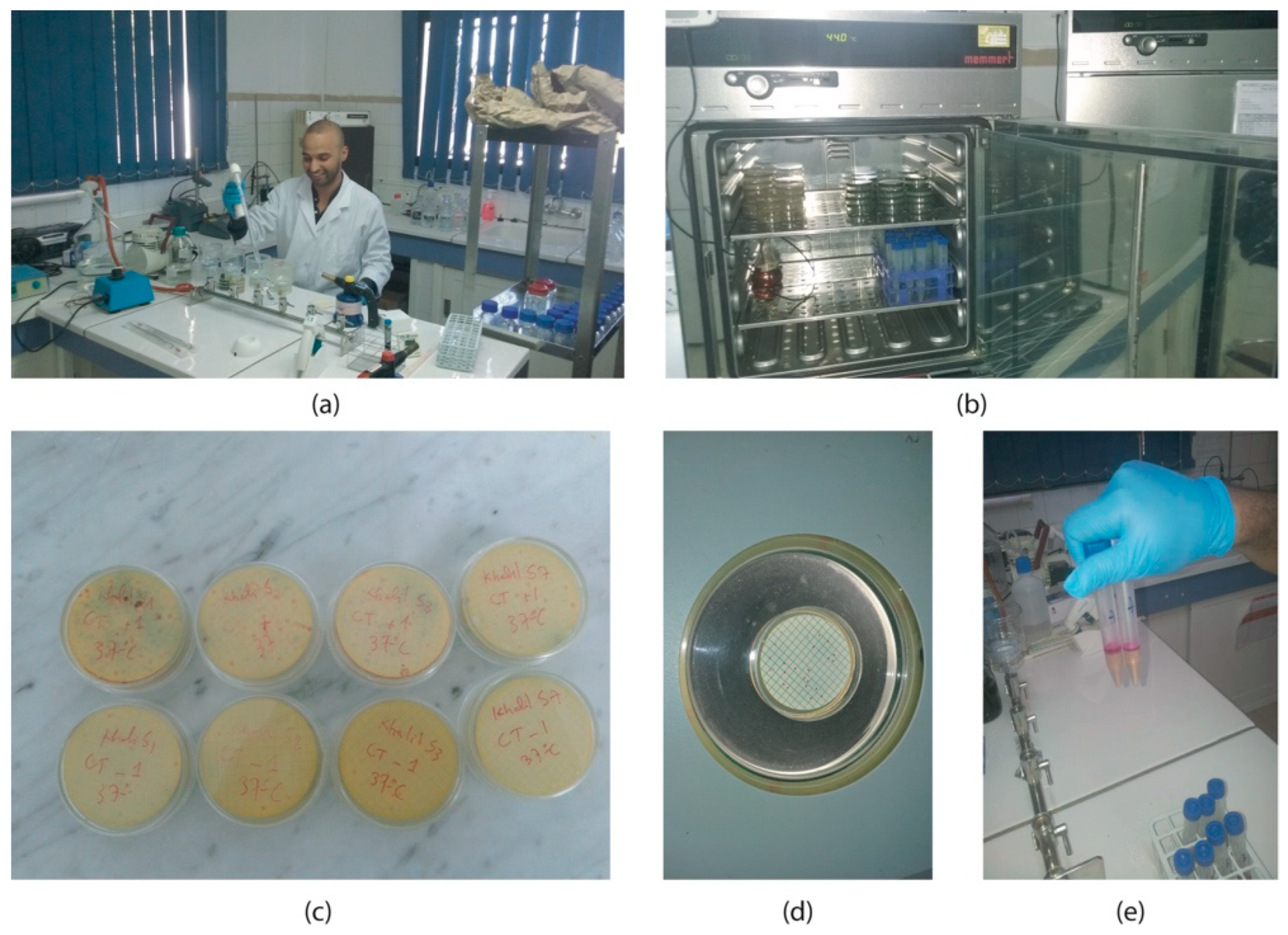
2.3. In-Situ Measurements

Based on their vulnerability to contamination [59,60,61,62], seven sampling points were selected along the west coast of Tangier for bacteriological analyses (Figure 1). At these points, samples of bathing water were collected the same day and time of images acquisition. Each sample was georeferenced using a GNSS receiver Leica 1200 (Hexagon AB, Stockholm, Sweden). The samples were performed from 50 cm up to 1 m depth using sterilized glass bottles. All samples were kept in cooled boxes during the transport and labeled with location and date, being analyzed within 24 h.
Bacterial pathogen analyses were performed following standard methods for: Total Coliforms (TC), Faecal Coliforms (FC) and Escherichia coli (E. coli) according to ISO 9308-1 [63] and Intestinal Enterococci (IE) according to ISO 7899-2 [64]. Water samples of 500 mL each were filtered (pore size: 0.45 µm) (Figure 3a), transferred onto selective media and then incubated at an appropriate temperature (Figure 3b). All measurements were confirmed before being determined as Colony Forming Units per 100 mL (CFU/100 mL) (Figure 3c–e). All bacteriological parameters measured were being compared to the Moroccan quality standards adopted by the Ministry of Energy, Mines, Water and Environment of Morocco (NM 03.7.200) [65].

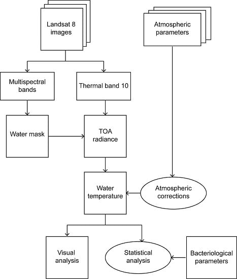
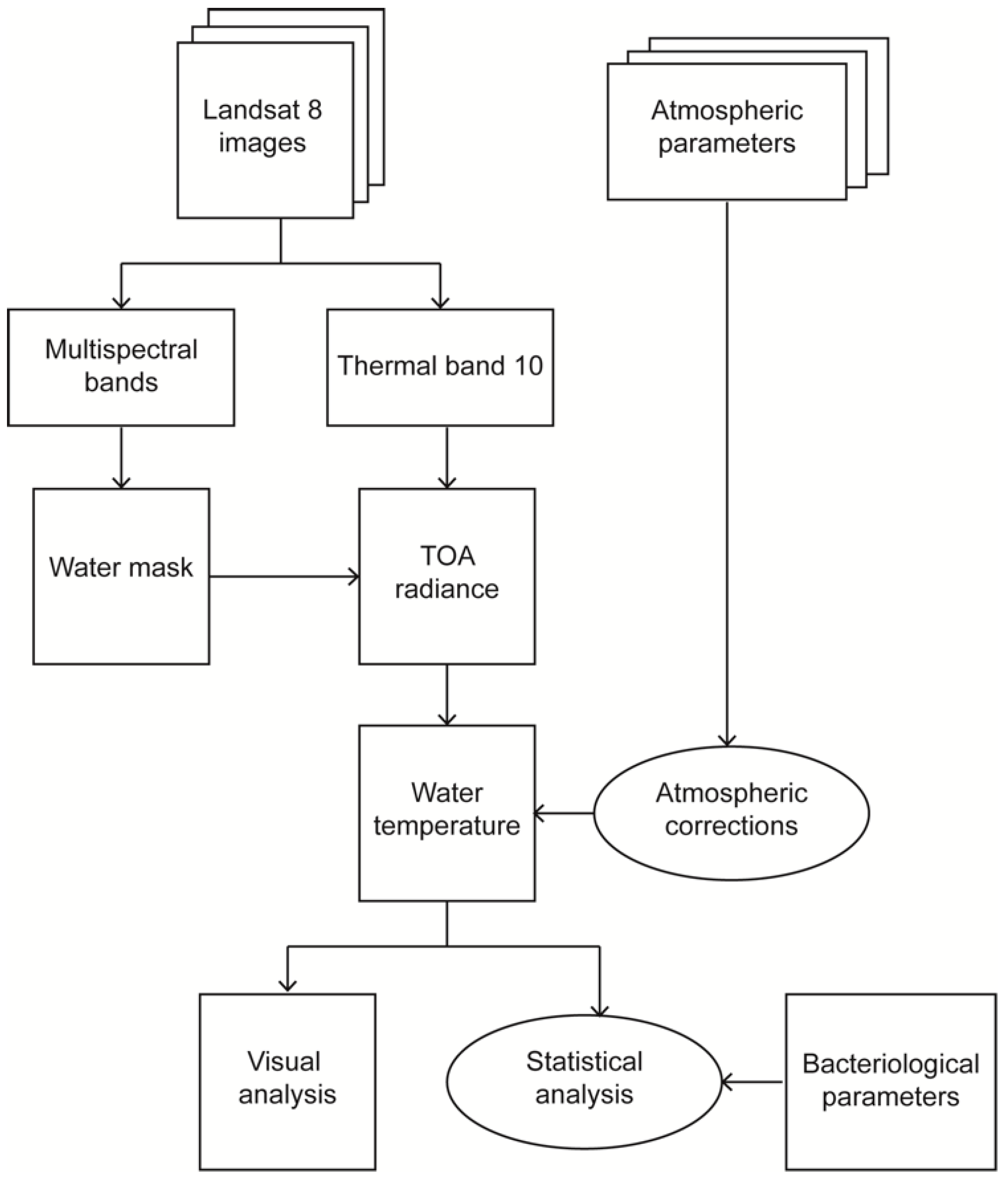
2.4. Study Procedure

In this study, the spatio-temporal pattern of thermal pollution was analyzed using Landsat 8 images through the steps shown in Figure 4 and explained in detail in the following sections.
Firstly, a water mask was generated using near infrared band from the OLI sensor. Land and sea surface were differentiated since the reflectance of water is nearly equal to zero in reflective infrared bands while reflectance of land cover is greater than water [66]. As a result, a water mask was applied to thermal band 10 to isolate water surface.

2.4.1. Water Surface Temperature Estimation

Digital Numbers (DNs) for each water pixel of thermal band 10 from Landsat 8 scenes were used to calculate Sea Surface Temperature (SST). Thermal infrared remote sensing measures the radiant energy emitted by the Earth’s surface, which makes it possible to compute the SST. By detecting the emitted radiation, it is possible to determine SST and map even small temperature variations [67]. For this, it was necessary to remove the effects of the atmosphere in order to use thermal band image for absolute temperature studies. The emitted signal from a target on the ground is both attenuated and enhanced by the atmosphere. Therefore, it is necessary to take into account the atmospheric interaction and use a Radiative Transfer Model (RTM) to remove atmospheric effects. A simplified radiative transfer equation to define apparent radiance received by a sensor is equal to Equation (1) [68]:
L s e n s o r , λ ( T ) = τ λ ϵ s , λ B λ ( T ) + L a t m , λ + τ λ ( 1 ϵ s , λ ) L a t m , λ
where:
  • L s e n s o r , λ : spectral at-sensor radiance (top of atmosphere) [ W · m 2 · sr 1 · μ m 1 ]
  • τ λ : atmospheric transmittance at λ [unitless].
  • ϵ s , λ : surface spectral emissivity [unitless].
  • B λ : ground radiance at a temperature T [K].
  • L a t m , λ : upwelling atmospheric radiance in a λ window [ W · m 2 · sr 1 · μ m 1 ].
  • L a t m , λ : downwelling atmospheric radiance in a λ window [ W · m 2 · sr 1 · μ m 1 ].
Landsat Level-1 thermal band was converted to spectral radiance at sensor ( L s e n s o r , λ ) using the radiance rescaling factor (Equation (2)) [69]:
L s e n s o r , λ = M L · Q c a l + A L
where:
  • M L : band-specific multiplicative rescaling factor.
  • A L : band-specific additive rescaling factor.
  • Q c a l : Quantized and calibrated standard product pixel values.
In this study, the emissivity of water was set as 0.9885 according to Simon et al. [70] The other three parameters; transmission, upwelling and downwelling radiance were calculated using the Atmospheric Correction Parameter Calculator (https://atmcorr.gsfc.nasa.gov) [71].
According to Plank’s law B λ can be expressed as Equation (3) [72]:
B λ = 2 h c 2 λ 5 ( exp ( h c / λ k T s ) 1 )
where:
  • T s : land/water surface temperature.
  • c : light speed, equal to 2.9979 × 10⁸ m/s.
  • h : Planck constant, equal to 6.6261 × 10⁻³⁴ J·s.
  • λ : wavelength.
Finally, sea surface temperature can be calculated by inverting Plank’s law as (Equation (4)) [73]:
T s = K 2 L n ( 1 + K 1 B λ )
where K 1   and K 2 are pre-launch calibration constant provided by the United States Geological Survey (USGS) [74].
In addition, to validate estimated SST values, a comparison with in-situ observed water temperature values using a thermometer were done, applying a simple regression model. These in-situ temperature measurements were performed at the same time as bathing water sampling, as described in Section 2.3.

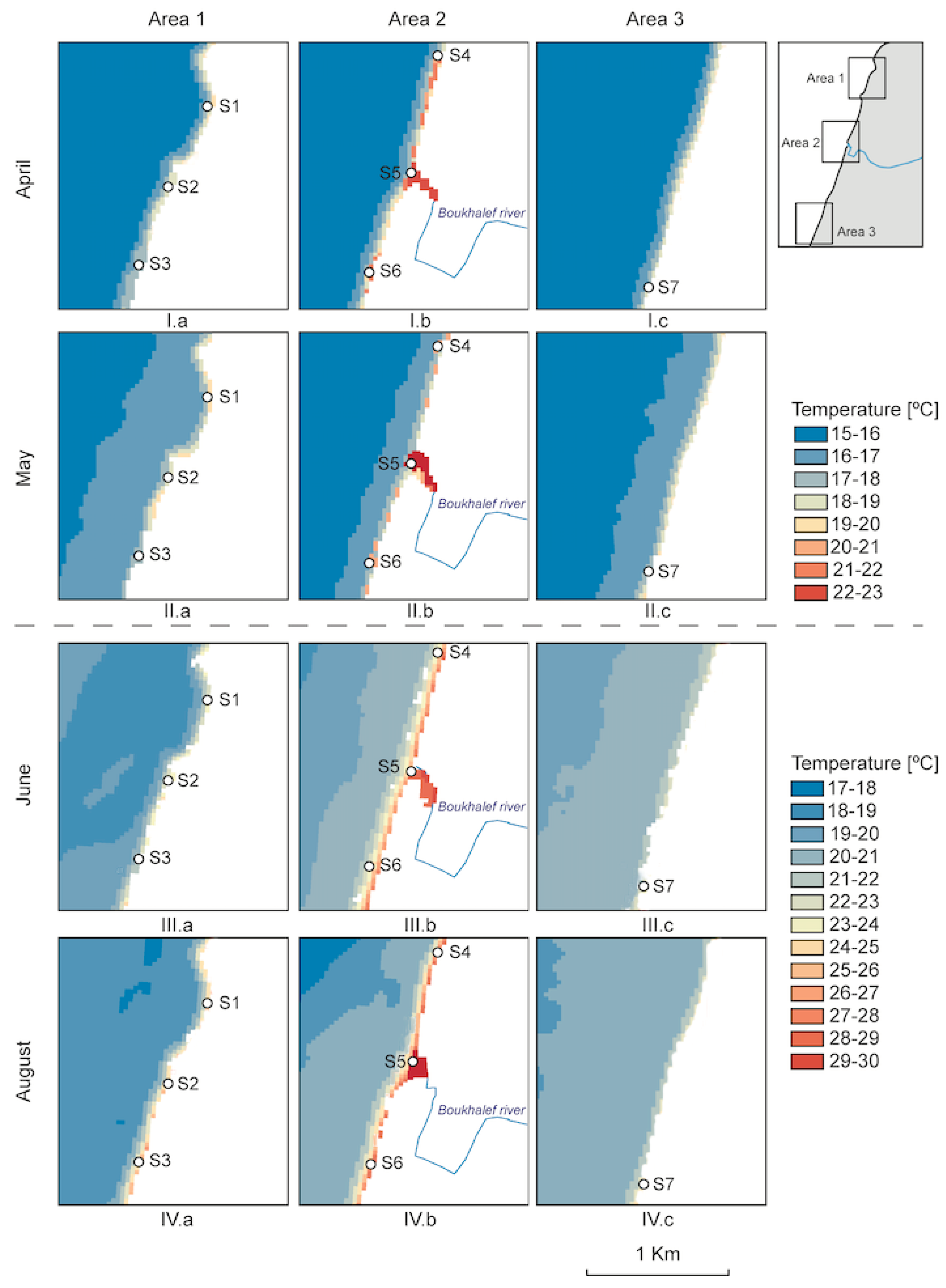
2.4.2. Spatio-Temporal Analysis
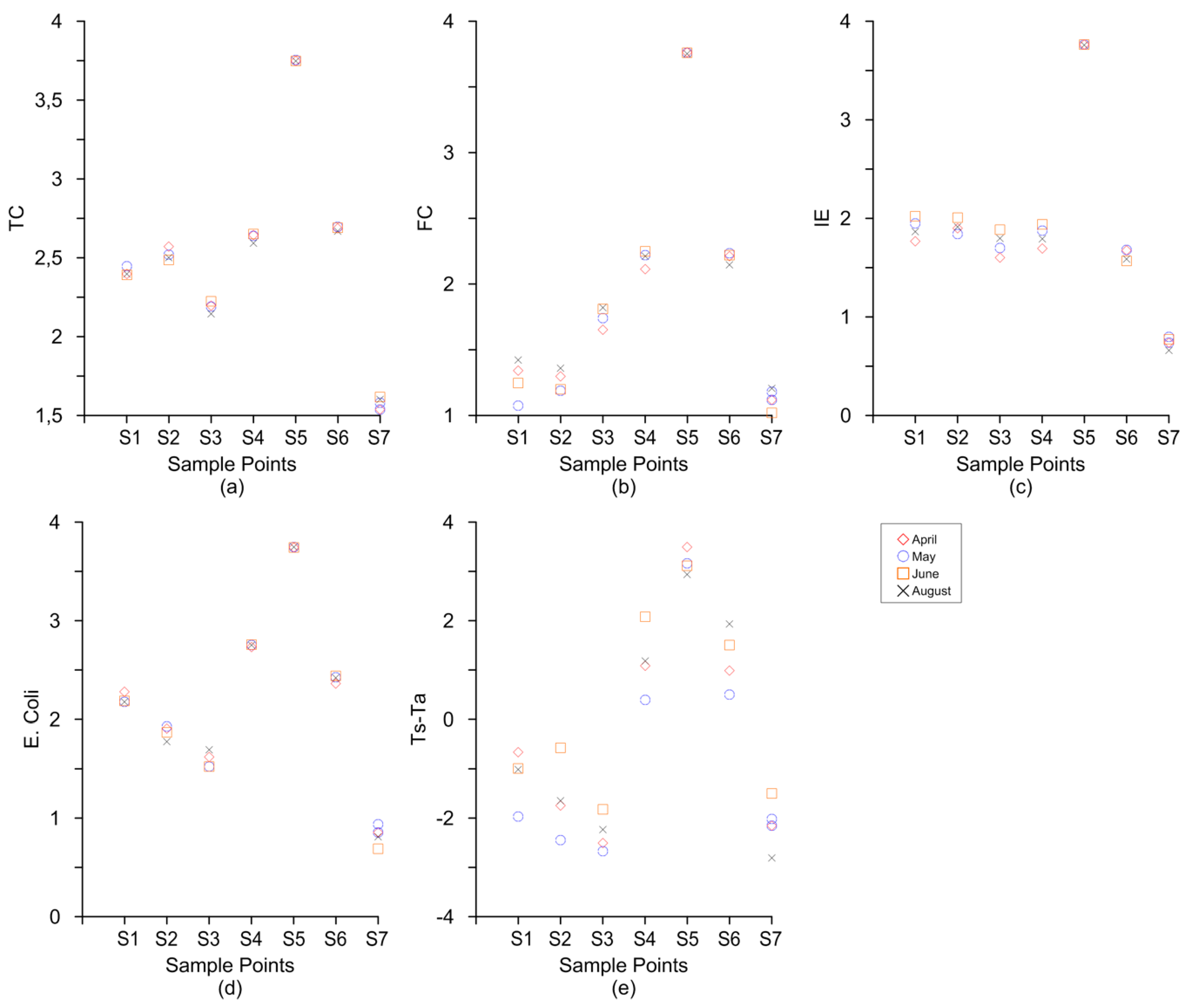
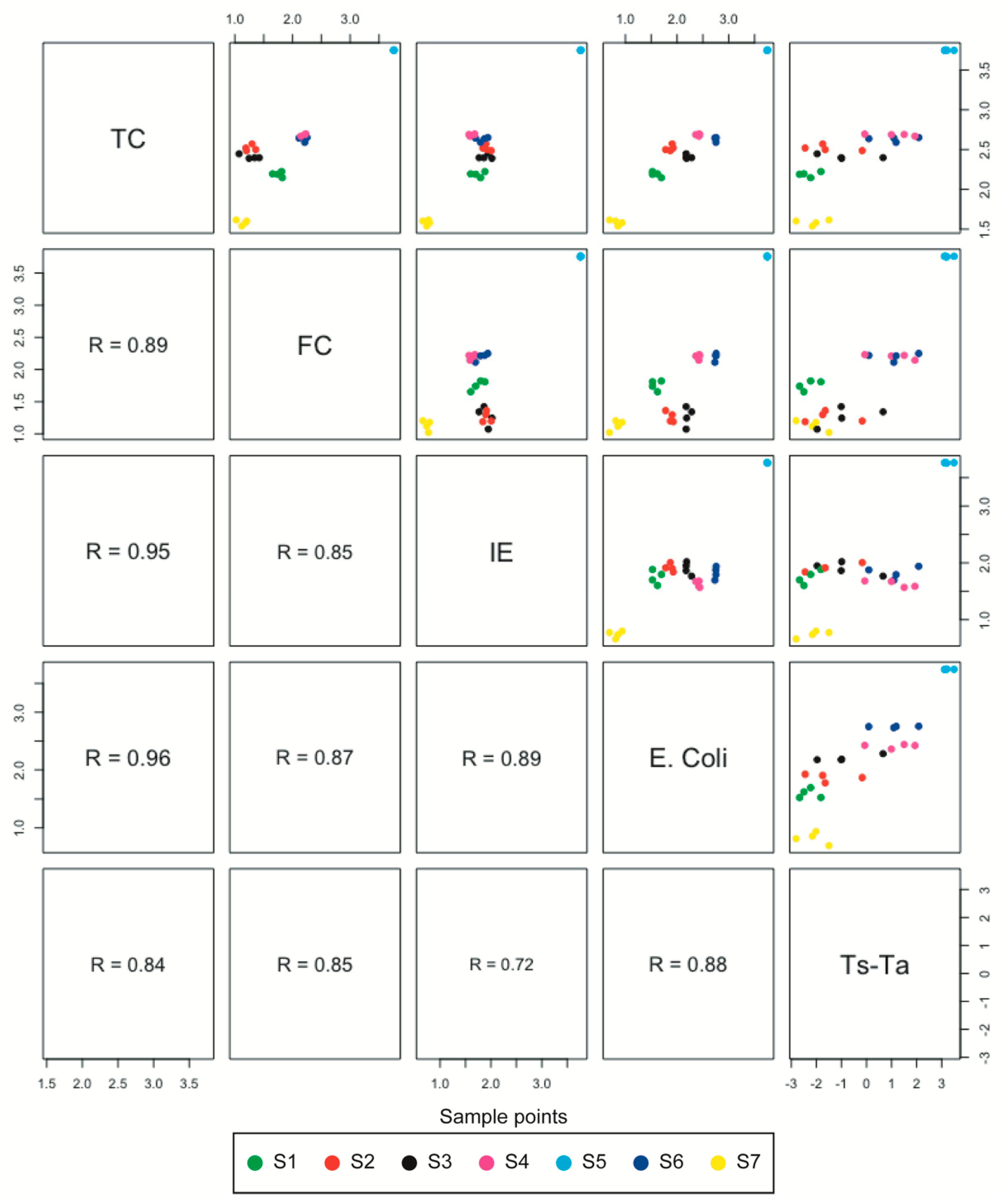
Sample points were characterized in terms of SST and bacteriological water quality. Variations between sample months and sample points, as well as possible correlations between bacteriological data and temperature, were analyzed. To remove seasonal cycle variations, we took into account the difference between sea and air temperature (Ts-Ta). First of all, a visual analysis was performed to detect temperature anomalies and the spatial distribution along the coastal bathing area. Following, the relationship between bacteriological parameters and Ts-Ta were evaluated and, finally, a model to explain the relationship between them was created. Statistical analyses were done using R [75].

3. Results

SST estimated values from Landsat 8 images and in-situ temperature measurements showed a significant correlation coefficient, range from 0.89–0.98 (p < 0.001). Errors were acceptable in all temperature images, root mean square error ranged from 0.67–0.75 °C, and showed good adjustment.
Figure 5 shows SST variations over four different months in three areas: Area 1 and Area 3 are located north and south of the Boukhalef river mouth respectively, Area 2 represents Jbila beach (S4), the Boukhalef river mouth (S5) and Sidikacem beach (S6). The SST was characterized by differentiation and variation of values from Area 1, 2 and 3 during spring and summer 2017. The highest temperature values were observed in Area 2 in the Boukhalef river mouth (S5). This area includes industrial zones that have an adverse impact on the quality of bathing waters [56].
As the distance to the mouth increases, the temperature in Area 1 and 3 decreases, which is proved by the lowest SST found in these areas in April and May, 17 °C and 18 °C respectively (Figure 5 I.a, II.a, I.c and II.c), and in June and August, 23 °C and 24 °C respectively (Figure 5 III.a, IV.a, III.c and IV.c). In Area 2, S5 showed the highest SST in all the months: April, 23.58 °C (Figure 5 I.b); May, 23.42 °C (Figure 5 II.b); June, 28.61 °C (Figure 5 III.b), and August, 29.75 °C (Figure 5 IV.b).
Table 2 summarizes the results of bacteriological in-situ measurements of the western coastal waters of Tangier per sampling point and month. Additionally, quality class of bathing waters, SST and air temperature are shown. Quality classes were assigned following Moroccan quality standards [65]. This standard defines class A as good quality, B as medium quality, C as temporally polluted and D as poor quality. A Davis Vantage Pro2 weather station (Davis Instrument Corp., Hayward, CA, USA) was used to monitor air temperature.
The in-situ measurements showed that the bathing waters of S5 were classified as class D while S4 was class C during the four months, reflecting the presence of industrial activities, tourism and important urbanization. On the other hand, S1, classified as B, and S2, S3 and S7 were classified as good quality (class A). Nonetheless, this bacteriological analysis result shows heavy bacterial contamination in agreement with those found by Bourouhou et al. (2018) [76] in the vicinity of Tangier region, north of Morocco, which is in close proximity to our study area. The high concentration of E. coli in S5 suggests that the local conditions favor the dispersion and reproduction of the E. coli at this point, due to the surface run off and Boukhalef river water quality. In addition, from a preliminary analysis of Table 2, it is observed that SST in the river mouth is always higher than the air temperature in S5. S4 and S6 showed SST similar to the air temperature in spring and a little higher in summer. On the other hand, samples distant from the river mouth (S1, S2, S3 and S7) always have SST values lower than the air temperature.
Figure 6 shows a comparative for each bacteriological parameter and Ts-Ta for each sample point and month. In-situ measurements showed that S7 had the lowest bacteriological concentration values while S5, close to the river mouth, had the highest values. In addition, S1, S2 and S3 were less contaminated than S4 and S6, in closer proximity to S5 (Figure 6a–d). Furthermore, Ts-Ta had similar behavior as pollutants. The highest values of Ts-Ta were found in S5; in agreement with the observed high bacteriological pollution during all months (Figure 6e) while S7, which represents Area 3 showed the lowest values during all months. Therefore, Ts-Ta showed behavior equal to the bacteriological concentration.
Figure 7 shows the relation of bacteriological parameters (TC, FC, IE and E. coli) and Ts-Ta for the seven sample points in the four months of sampling. Comparing the relationship between bacteriological parameters, they showed an adequate positive correlation between 0.85 (TC and IE) and 0.96 (TC and E. coli) (level of significance p < 0.05). From the comparison of the different scatterplots between pollutants, it was observed that in all of them, the lowest concentration was at point S7. On the other hand, S5 showed the highest concentration. This relationship between all bacteriological parameters was logical because they appeared in the same medium, in the same biological conditions and for the same cause. In addition, their presence is confirmed by the existence of each other. Comparison between bacteriological parameters and Ts-Ta showed also a positive correlation range from 0.72 (IE and Ts-Ta) to 0.88 (E. coli and Ts-Ta) (level of significance p < 0.05). Consequently, it can be assumed that as Ts-Ta increases, the concentration of contaminants in the water also increases.
It is agreed that Escherichia coli is the most commonly used bacterial indicator of fecal pollution [77]. Figure 8 shows in detail the relation between Ts-Ta and Escherichia coli. Both variables showed a lineal relationship with a correlation coefficient higher than 0.85 (p-value < 0.05). Figure 9 shows a diagnosis of the lineal model. First of all, residuals are equally spread around dot horizontal line (Figure 9a). It indicates there is a linear relationship between fitted values and residuals. Normal Q-Q plot (Figure 9b) shows how residuals are normally distributed, following a straight line not being deviated severely. Shapiro–Wilk normality test was applied to residuals getting W = 0.9568 and p-value = 0.292. From this result, the p-value is higher than 0.05 and therefore residual distribution is not significantly different from normal distribution. Figure 9c shows how residuals are spread equally along the ranges of predictors, and therefore have equal variance. Finally, extreme values used in this value are not influential to determine regression model. Figure 9d shows how any sample is outside the Cook’s distance and therefore the regression results will not be altered if any measurement is excluded.
Although these results allow information at a regional scale, it is necessary to improve the temporal resolution of the data source. The changing conditions of coastal systems demand updated information as time passes. Earth observation programs with medium spatial resolution, such as Landsat, offer information every 15 days, therefore it is not possible to have daily data. Moreover, it is necessary to take into account the presence of clouds masking the working area. Other programs, e.g., MODIS, offer daily surface temperature with one-kilometer spatial resolution, as such it is not adequate to monitor small areas of bathing water. These first results invite continuing research in order to develop a predictive model for determining fecal pollutant concentration in bathing waters by remote satellite images. This predictive model will be based on in-situ measurements, wind models and remote sensing thermal images among others. It will allow a reduction of temporal and economic costs when sampling the field. Moreover, it will permit obtaining up-to-date information supporting policies aimed at the conservation of the environment and creating a surveillance system, allowing the creation of alerts for high concentrations of pollutants. Finally, it is possible to develop applications that inform the bather of the quality of the bathing waters, favoring the development of tourism activities.

4. Conclusions

The results of the present study showed a high fecal pollution concentration and SST values in Jbila and Sidikacem beach waters on the west coast of Tangier where discharges of the Boukhalef river meet the ocean after it runs along a heavily industrialized area. In addition, low fecal pollution concentration and SST values were located in other beaches moving away from the Boukhalef river mouth. Therefore, a significant correlation between water remote sensing temperature from Landsat 8 images and different bacteriological parameters were found.
Also, the study presents a relatively simple model based on SST that can assist beach closure decision makers. The regression model provides evaluation and detection of potential pollution in the coast. Therefore, remotely sensed water temperature data can provide low cost, yet high temporal and spatial resolution information for the assessment and regular monitoring of this region’s marine water quality indicator. This is relevant because identification of certain bacterial groups and individual species is very costly.
Hence, the study demonstrates the potential of remote sensing data as a useful indicator of bacterial pollution in bathing waters in general, and in particular the importance of using thermal satellite images as well as Landsat 8 TIRS bands in determining bathing waters’ quality, which could be a cost-effective technique compared to classical methods.
Thereby, remote sensing images can provide a basis for modeling bathing water quality, being a starting point for further research related to water quality objectives. Results will support decision makers in establishing adequate policies to prevent environmental hazards and achieving good water quality in the west coast of Tangier, Morocco in the future.
The present study should be taken as a preliminary result. Some objectives following this study are as follows:
-
In relation to the evaluation of water consumer safety, more robust and complex models have to be developed, such as neuronal networks. These future models will manage information from different sources, providing information to support decision makers based on complex classifications.
-
A dedicated campaign in the western coastal waters of Tangier, Morocco should be established to provide a huge amount of necessary data as input to identify he network’s rules.
-
Real-time modeling of bacteria concentrations is necessary as it aids decision makers in their judgment of bathing water. This new service will be supported by predicted models based on remote sensing thermal images and other data sources including, but not limited to, wind models and in-situ measurements.
Finally, this research represents an additional step towards the development of this type of model based on additional data sets from coastal observing systems or weather forecast.

Author Contributions

E.K.C. and F.S. conceived and designed and performed the experiment; E.K.C., F.S. and F.J.M.-C. analyzed the data; E.K.C. and F.J.M.-C. wrote the paper.

Funding

This research did not receive any specific grant from funding agencies in the public, commercial, or not-for-profit sectors.

Acknowledgments

The authors would like to thank all researchers who have worked hard to advance knowledge and improve outcomes of seawater quality evaluation. This study was supported by the National Office of Food Safety (ONSSA) and the National Office of Drinking Water (ONEP) in Tangier, Morocco by providing the materials and equipment for Bacteriological and physico-chemical analysis.

Conflicts of Interest

The authors declare no conflict of interest.

References

  1. Sloggett, D.; Srokosz, M.; Aiken, J.; Boxall, S. Operational Uses of Ocean Colour Data-Perspectives for the OCTOPUS Programme; Balkema Publishers: Rotterdam, The Netherlands, 1995. [Google Scholar]
  2. Gravari-Barbas, M.; Jacquot, S. Atlas Mondial du Tourisme et des Loisirs; Autrement: Paris, France, 2018. [Google Scholar]
  3. Le Tixerant, M. Human Activities Dynamic in Coastal Sea. Application to the Iroise Sea. Ph.D. Thesis, Université de Bretagne Occidentale, Brest, France, 2004. [Google Scholar]
  4. Moubarrad, F.-Z.L.; Assobhei, O. The health effects of wastewater on the prevalence of ascariasis among the children of the discharge zone of El Jadida, Morocco. Int. J. Environ. Health Res. 2005, 15, 135–142. [Google Scholar] [CrossRef]
  5. Paraskevas, P.A.; Giokas, D.L.; Lekkas, T.D. Wastewater management in coastal urban areas: The case of Greece. Water Sci. Technol. 2002, 46, 177–186. [Google Scholar] [CrossRef] [PubMed]
  6. Selvakumar, A.; Borst, M. Variation of microorganism concentrations in urban stormwater runoff with land use and seasons. J. Water Health 2006, 4, 109–124. [Google Scholar] [CrossRef]
  7. Burton, G.A., Jr.; Pitt, R. Stormwater Effects Handbook: A Toolbox for Watershed Managers, Scientists, and Engineers; CRC Press: Boca Raton, FL, USA, 2001. [Google Scholar]
  8. Kosenius, A.-K. Heterogeneous preferences for water quality attributes: The case of eutrophication in the Gulf of Finland, the Baltic Sea. Ecol. Econ. 2010, 69, 528–538. [Google Scholar] [CrossRef]
  9. Ritchie, J.C.; Schiebe, F.R. Water quality. In Remote Sensing in Hydrology and Water Management; Springer: Berlin/Heidelberg, Germany, 2000; pp. 287–303. [Google Scholar]
  10. CRWN. Colorado River Watch Network Water Quality Monitoring; CRWN: Austin, TX, USA, 2012. [Google Scholar]
  11. Gholizadeh, M.; Melesse, A.; Reddi, L. A Comprehensive Review on Water Quality Parameters Estimation Using Remote Sensing Techniques. Sensors 2016, 16, 1298. [Google Scholar] [CrossRef] [PubMed]
  12. Mohebbi, M.R.; Saeedi, R.; Montazeri, A.; Vaghefi, K.A.; Labbafi, S.; Oktaie, S.; Abtahi, M.; Mohagheghian, A. Assessment of water quality in groundwater resources of Iran using a modified drinking water quality index (DWQI). Ecol. Indic. 2013, 30, 28–34. [Google Scholar] [CrossRef]
  13. Boyacioglu, H. Development of a water quality index based on a European classification scheme. Water SA 2007, 33. [Google Scholar] [CrossRef]
  14. Pietrucha-Urbanik, K. Assessment model application of water supply system management in crisis situations. Glob. Nest J. 2014, 16, 893–900. [Google Scholar]
  15. Pietrucha-Urbanik, K.; Tchorzewska-Cieslak, B. Water Supply System operation regarding consumer safety using Kohonen neural network. In Safety, Reliability and Risk Analysis: Beyond the Horizon; Taylor & Francis Group: London, UK, 2014; pp. 1115–1120. [Google Scholar]
  16. Thomas, A.; Byrne, D.; Weatherbee, R. Coastal sea surface temperature variability from Landsat infrared data. Remote Sens. Environ. 2002, 81, 262–272. [Google Scholar] [CrossRef]
  17. Duan, W.; He, B.; Takara, K.; Luo, P.; Nover, D.; Sahu, N.; Yamashiki, Y. Spatiotemporal evaluation of water quality incidents in Japan between 1996 and 2007. Chemosphere 2013, 93, 946–953. [Google Scholar] [CrossRef]
  18. Morel, A.; Prieur, L. Analysis of variations in ocean color 1. Limnol. Oceanogr. 1977, 22, 709–722. [Google Scholar] [CrossRef]
  19. Anding, D.; Kauth, R. Estimation of sea surface temperature from space. Remote Sens. Environ. 1970, 1, 217–220. [Google Scholar] [CrossRef]
  20. Tilstone, G.H.; Lotliker, A.A.; Miller, P.I.; Ashraf, P.M.; Kumar, T.S.; Suresh, T.; Ragavan, B.R.; Menon, H.B. Assessment of MODIS-Aqua chlorophyll-a algorithms in coastal and shelf waters of the eastern Arabian Sea. Cont. Shelf Res. 2013, 65, 14–26. [Google Scholar] [CrossRef]
  21. Santini, F.; Alberotanza, L.; Cavalli, R.M.; Pignatti, S. A two-step optimization procedure for assessing water constituent concentrations by hyperspectral remote sensing techniques: An application to the highly turbid Venice lagoon waters. Remote Sens. Environ. 2010, 114, 887–898. [Google Scholar] [CrossRef]
  22. Sudheer, K.P.; Chaubey, I.; Garg, V. Lake water quality assessment from Landsat thematic mapper data using neural network: An approch to optimal band combination selection. J. Am. Water Resour. Assoc. 2006, 42, 1683–1695. [Google Scholar] [CrossRef]
  23. He, B.; Oki, K.; Wang, Y.; Oki, T. Using remotely sensed imagery to estimate potential annual pollutant loads in river basins. Water Sci. Technol. 2009, 60, 2009–2015. [Google Scholar] [CrossRef]
  24. Giardino, C.; Bresciani, M.; Cazzaniga, I.; Schenk, K.; Rieger, P.; Braga, F.; Matta, E.; Brando, V. Evaluation of Multi-Resolution Satellite Sensors for Assessing Water Quality and Bottom Depth of Lake Garda. Sensors 2014, 14, 24116–24131. [Google Scholar] [CrossRef] [Green Version]
  25. Brando, V.E.; Dekker, A.G. Satellite hyperspectral remote sensing for estimating estuarine and coastal water quality. IEEE Trans. Geosci. Remote Sens. 2003, 41, 1378–1387. [Google Scholar] [CrossRef]
  26. Eric, S.; David, B.; Mark, D.B.; Steven, D.G. Flow, food supply and acorn barnacle population dynamics. Mar. Ecol. Prog. Ser. 1994, 104, 49–62. [Google Scholar]
  27. Donlon, C.J.; Minnett, P.J.; Gentemann, C.; Nightingale, T.J.; Barton, I.J.; Ward, B.; Murray, M.J. Toward Improved Validation of Satellite Sea Surface Skin Temperature Measurements for Climate Research. J. Clim. 2002, 15, 353–369. [Google Scholar] [CrossRef] [Green Version]
  28. Tang, D.; Kester, D.R.; Wang, Z.; Lian, J.; Kawamura, H. AVHRR satellite remote sensing and shipboard measurements of the thermal plume from the Daya Bay, nuclear power station, China. Remote Sens. Environ. 2003, 84, 506–515. [Google Scholar] [CrossRef] [Green Version]
  29. Ahn, Y.-H.; Shanmugam, P.; Lee, J.-H.; Kang, Y.Q. Application of satellite infrared data for mapping of thermal plume contamination in coastal ecosystem of Korea. Mar. Environ. Res. 2006, 61, 186–201. [Google Scholar] [CrossRef]
  30. Ouzounov, D.; Bryant, N.; Logan, T.; Pulinets, S.; Taylor, P. Satellite thermal IR phenomena associated with some of the major earthquakes in 1999–2003. Phys. Chem. Earth Parts ABC 2006, 31, 154–163. [Google Scholar] [CrossRef]
  31. Peñaflor, E.L.; Skirving, W.J.; Strong, A.E.; Heron, S.F.; David, L.T. Sea-surface temperature and thermal stress in the Coral Triangle over the past two decades. Coral Reefs 2009, 28, 841–850. [Google Scholar] [CrossRef]
  32. Liu, G.; Heron, S.; Eakin, C.; Muller-Karger, F.; Vega-Rodriguez, M.; Guild, L.; De La Cour, J.; Geiger, E.; Skirving, W.; Burgess, T.; et al. Reef-Scale Thermal Stress Monitoring of Coral Ecosystems: New 5-km Global Products from NOAA Coral Reef Watch. Remote Sens. 2014, 6, 11579–11606. [Google Scholar] [CrossRef] [Green Version]
  33. Hadjimitsis, D.G.; Hadjimitsis, M.G.; Clayton, C.; Clarke, B.A. Determination of Turbidity in Kourris Dam in Cyprus Utilizing Landsat TM Remotely Sensed Data. Water Resour. Manag. 2006, 20, 449–465. [Google Scholar] [CrossRef]
  34. Mallast, U.; Siebert, C.; Wagner, B.; Sauter, M.; Gloaguen, R.; Geyer, S.; Merz, R. Localisation and temporal variability of groundwater discharge into the Dead Sea using thermal satellite data. Environ. Earth Sci. 2013, 69, 587–603. [Google Scholar] [CrossRef] [Green Version]
  35. Casciello, D.; Lacava, T.; Pergola, N.; Tramutoli, V. Robust Satellite Techniques for oil spill detection and monitoring using AVHRR thermal infrared bands. Int. J. Remote Sens. 2011, 32, 4107–4129. [Google Scholar] [CrossRef]
  36. Salama, Y.; Chennaoui, M.; Mountadar, M.; Rihani, M.; Assobhei, O. The physicochemical and bacteriological quality and environmental risks of raw sewage rejected in the coast of the city of El Jadida (Morocco). Carpathian J. Earth Environ. Sci. 2013, 8, 39–48. [Google Scholar]
  37. Moubarrad, F.-Z.L.; Assobhei, O. Health risks of raw sewage with particular reference to Ascaris in the discharge zone of El Jadida (Morocco). Desalination 2007, 215, 120–126. [Google Scholar] [CrossRef]
  38. European Union. Directive 2006/7/EC of the European Parliament and of the Council of 15 February 2006 concerning the management of bathing water quality and repealing Directive 76/160/EEC. Off. J. Eur. Union 2006, 64, 14. [Google Scholar]
  39. Callahan, K.M.; Taylor, D.J.; Sobsey, M.D. Comparative survival of hepatitis A virus, poliovirus and indicator viruses in geographically diverse seawaters. Water Sci. Technol. 1995, 31, 189–193. [Google Scholar] [CrossRef]
  40. Craig, D.L.; Fallowfield, H.J.; Cromar, N.J. Use of microcosms to determine persistence of Escherichia coli in recreational coastal water and sediment and validation with in situ measurements. J. Appl. Microbiol. 2004, 96, 922–930. [Google Scholar] [CrossRef] [Green Version]
  41. Mallin, M.A.; Williams, K.E.; Esham, E.C.; Lowe, R.P. Effect of human development on bacteriological water quality in coastal watersheds. Ecol. Appl. 2000, 10, 1047–1056. [Google Scholar] [CrossRef]
  42. Ekercin, S. Water quality retrievals from high resolution IKONOS multispectral imagery: A case study in Istanbul, Turkey. Water. Air. Soil Pollut. 2007, 183, 239–251. [Google Scholar] [CrossRef]
  43. Fournier, M. L’apport de l’imagerie satellitale à la surveillance maritime. Contribution géographique et géopolitique. Ph.D. Thesis, Université Paul Valéry-Montpellier III, Montpellier, France, 2012. [Google Scholar]
  44. Shaban, A. Use of satellite images to identify marine pollution along the Lebanese coast. Environ. Forensics 2008, 9, 205–214. [Google Scholar] [CrossRef]
  45. Vignolo, A.; Pochettino, A.; Cicerone, D. Water quality assessment using remote sensing techniques: Medrano Creek, Argentina. J. Environ. Manag. 2006, 81, 429–433. [Google Scholar] [CrossRef]
  46. Kelsey, R.H.; Scott, G.I.; Porter, D.E.; Siewicki, T.C.; Edwards, D.G. Improvements to Shellfish Harvest Area Closure Decision Making Using GIS, Remote Sensing, and Predictive Models. Estuaries Coasts 2010, 33, 712–722. [Google Scholar] [CrossRef]
  47. Kim, J.H.; Grant, S.B. Public Mis-Notification of Coastal Water Quality: A Probabilistic Evaluation of Posting Errors at Huntington Beach, California. Environ. Sci. Technol. 2004, 38, 2497–2504. [Google Scholar] [CrossRef] [PubMed] [Green Version]
  48. Siewicki, T.C.; Pullaro, T.; Pan, W.; McDaniel, S.; Glenn, R.; Stewart, J. Models of total and presumed wildlife sources of fecal coliform bacteria in coastal ponds. J. Environ. Manag. 2007, 82, 120–132. [Google Scholar] [CrossRef] [PubMed]
  49. Kelsey, H.; Porter, D.E.; Scott, G.; Neet, M.; White, D. Using geographic information systems and regression analysis to evaluate relationships between land use and fecal coliform bacterial pollution. J. Exp. Mar. Biol. Ecol. 2004, 298, 197–209. [Google Scholar] [CrossRef]
  50. Wright, R.C. A Comparison of the Levels of Faecal Indicator Bacteria in Water and Human Faeces in a Rural Area of a Tropical Developing Country (Sierra Leone). J. Hyg. 1982, 89, 69–78. [Google Scholar] [CrossRef]
  51. Viau, E.J.; Goodwin, K.D.; Yamahara, K.M.; Layton, B.A.; Sassoubre, L.M.; Burns, S.L.; Tong, H.-I.; Wong, S.H.C.; Lu, Y.; Boehm, A.B. Bacterial pathogens in Hawaiian coastal streams—Associations with fecal indicators, land cover, and water quality. Water Res. 2011, 45, 3279–3290. [Google Scholar] [CrossRef] [PubMed]
  52. Maillard, P.; Pinheiro Santos, N.A. A spatial-statistical approach for modeling the effect of non-point source pollution on different water quality parameters in the Velhas river watershed—Brazil. J. Environ. Manag. 2008, 86, 158–170. [Google Scholar] [CrossRef] [PubMed]
  53. Sheppard, D.; Tsegaye, T.D.; Tadesse, W.; McKay, D.; Coleman, T.L. The application of remote sensing, geographic information systems, and Global Positioning System technology to improve water quality in northern Alabama. In Proceedings of the IGARSS 2001. Scanning the Present and Resolving the Future. IEEE 2001 International Geoscience and Remote Sensing Symposium (Cat. No.01CH37217), Sydney, NSW, Australia, 9–13 July 2001; Volume 3, pp. 1291–1293. [Google Scholar]
  54. EEA. Horizon 2020 Mediterranean Report Annex 4; Publications Office of the European Union: Luxembourg, 2014; p. 36. [Google Scholar]
  55. Cherif, E.K.; Salmoun, F. Diagnostic of the Environmental Situation of the West Coast of Tangier. J. Mater. Environ. Sci. 2018, 8, 631–640. [Google Scholar]
  56. Ahmaruzzaman, M. Industrial wastes as low-cost potential adsorbents for the treatment of wastewater laden with heavy metals. Adv. Colloid Interface Sci. 2011, 166, 36–59. [Google Scholar] [CrossRef]
  57. Barsi, J.; Lee, K.; Kvaran, G.; Markham, B.; Pedelty, J. The spectral response of the Landsat-8 operational land imager. Remote Sens. 2014, 6, 10232–10251. [Google Scholar] [CrossRef]
  58. Irons, J.R.; Dwyer, J.L.; Barsi, J.A. The next Landsat satellite: The Landsat data continuity mission. Remote Sens. Environ. 2012, 122, 11–21. [Google Scholar] [CrossRef]
  59. Ministry of the Environment. Rapport Analytique du Surveillance de la Qualité des eaux de Baignade; Ministry of the Environment: Morocco, 2013.
  60. Ministry of the Environment. Rapport Analytique du Surveillance de la Qualité des eaux de Baignade; Ministry of the Environment: Morocco, 2014.
  61. Ministry of the Environment. Rapport Analytique du Surveillance de la Qualité des eaux de Baignade; Ministry of the Environment: Morocco, 2015.
  62. Ministry of the Environment. Rapport Analytique du Surveillance de la Qualité des eaux de Baignade; Ministry of the Environment: Morocco, 2016.
  63. ISO Water Quality—Enumeration of Escherichia Coli and Coliform Bacteria—Part 1: Membrane Filtration Method for Waters with Low Bacterial Background Flora; ISO: Geneva, Switzerland, 2014.
  64. ISO Water Quality—Research and Enumeration of Intestinal Enterococci—Part 2: Membrane Filtration Method for Waters; ISO: Geneva, Switzerland, 2000.
  65. IMANOR. Standards for Monitoring Bathing Water Quality; IMANOR: Rabat, Morocco, 1998.
  66. Alesheikh, A.A.; Ghorbanali, A.; Nouri, N. Coastline change detection using remote sensing. Int. J. Environ. Sci. Technol. 2007, 4, 61–66. [Google Scholar] [CrossRef] [Green Version]
  67. Jensen, J.R. Remote Sensing of Environment: An Earth Resource. Saddle River; Prentice-Hall, Inc.: Englewood Cliffs, NJ, USA, 2000. [Google Scholar]
  68. Mao, K.; Qin, Z.; Shi, J.; Gong, P. Research of Split-Window Algorithm on the MODIS. Geomat. Inf. Sci. Wuhan Univ. 2005, 30, 703–707. [Google Scholar]
  69. Zanter, K. Landsat 8 Dta Users Handbook; Department of the Interior U.S. Geological Survey: Sioux Falls, SD, USA, 2018; Volume Version 3.0.
  70. Simon, R.N.; Tormos, T.; Danis, P.-A. Retrieving water surface temperature from archive Landsat thermal infrared data: Application of the mono-channel atmospheric correction algorithm over two freshwater reservoirs. Int. J. Appl. Earth Obs. Geoinf. 2014, 30, 247–250. [Google Scholar] [CrossRef]
  71. Barsi, J.A.; Barker, J.L.; Schott, J.R. An atmospheric correction parameter calculator for a single thermal band earth-sensing instrument. In Proceedings of the IGARSS 2003 IEEE International Geoscience and Remote Sensing Symposium. Proceedings (IEEE Cat. No. 03CH37477), Toulouse, France, 21–25 July 2003; Volume 5, pp. 3014–3016. [Google Scholar]
  72. Yu, X.; Guo, X.; Wu, Z. Land surface temperature retrieval from Landsat 8 TIRS—Comparison between radiative transfer equation-based method, split window algorithm and single channel method. Remote Sens. 2014, 6, 9829–9852. [Google Scholar] [CrossRef]
  73. Chander, G.; Markham, B. Revised Landsat-5 TM radiometric calibration procedures and postcalibration dynamic ranges. IEEE Trans. Geosci. Remote Sens. 2003, 41, 2674–2677. [Google Scholar] [CrossRef]
  74. Barsi, J.; Schott, J.; Hook, S.; Raqueno, N.; Markham, B.; Radocinski, R. Landsat-8 thermal infrared sensor (TIRS) vicarious radiometric calibration. Remote Sens. 2014, 6, 11607–11626. [Google Scholar] [CrossRef]
  75. R Core Team. R: A Language and Environment for Statistical Computing; R Foundation for Statistical Computing: Vienna, Austria, 2016. [Google Scholar]
  76. Bourouhou, I.; Salmoun, F.; Gedik, Y. Characteristics of Mediterranean Sea Water in Vicinity of Tangier Region, North of Morocco. Multidiscip. Digit. Publ. Inst. Proc. 2018, 2, 1291. [Google Scholar] [CrossRef]
  77. Edberg, S.C.L.; Rice, E.W.; Karlin, R.J.; Allen, M.J. Escherichia coli: The best biological drinking water indicator for public health protection. J. Appl. Microbiol. 2000, 88, 106S–116S. [Google Scholar] [CrossRef]
Figure 1. Study area in the west coast of Tangier, northern Morocco with locations of seven sampling points, Bouakhelf river and industrial zones.
Remotesensing 11 00972 g001
Figure 2. The Boukhalef river stream—industrial wastewater channels (a) discharging into the Boukhalef river (b) which meets the Atlantic Ocean near Sidikacem beach in (c) the west coast of Tangier.
Remotesensing 11 00972 g002
Figure 3. Different stages of bacteriological analysis: (a) filtration of water, (b) incubation (e), (c,d) lecture of the results and (e) confirmation.
Remotesensing 11 00972 g003
Figure 4. Flowchart of monitoring bathing water with Landsat 8 thermal bands.
Remotesensing 11 00972 g004
Figure 5. Water Surface Temperature [°C] of the west coast of Tangier; in spring (April and May) and summer (June and August) 2017 in the three areas in relation with sample points. Months: April (I), May (II), June (III) and August (IV). Areas: area 1 (a), area 2 (b) and area 3 (c).
Remotesensing 11 00972 g005
Figure 6. Evolution of bacteriological parameters and sample points by month for (a) Total Coliforms (TC), (b) Faecal Coliforms (FC), (c) Intestital Enterococci (IE), (d) Escherichia coli (E. coli) and (e) Ts-Ta.
Remotesensing 11 00972 g006
Figure 7. Multi scatter plot of bacteriological parameters (Total Coliforms (TC), Faecal Coliforms, Intestital Enterococci (IE) and Escherichia coli (E. coli) and Surface temperature minus air temperature (Ts-Ta).
Remotesensing 11 00972 g007
Figure 8. Linear regression analysis of Ts-Ta versus E. coli.
Remotesensing 11 00972 g008
Figure 9. Residual analysis lineal model Ts-Ta and E. coli: (a) Residuals versus fitted values, (b) normality of residuals, (c) scale-location and (d) leverage versus residuals.
Remotesensing 11 00972 g009
Table 1. Landsat 8 images. Timing is referenced to the Greenwich Mean Time (GMT).
Landsat IDPathRowDateTime
LC08_L1TP_202035_20170414_20170501_01_T12023514-APR-1710:56:08
LC08_L1TP_202035_20170516_20170525_01_T12023516-MAY-1711:02:08
LC08_L1TP_202035_20170617_20170629_01_T12023517-JUN-1711:02:24
LC08_L1TP_201035_20170813_20170825_01_T12013513-AUG-1710:57:04
Table 2. Bacteriological analysis results of the bathing water samples, quality class, air temperature (Ta) and Sea Surface Temperature (SST).
DateSample PointsTC
[UFC/100 mL]
FC
[UFC/100 mL]
IE
[UFC/100 mL]
E. coli
[UFC/100 mL]
Quality Class *Ta [°C]SST [°C]
April1250.0021.9858.41191.20B21.0920.75
2372.5919.8079.3380.52A18.34
3156.7745.0740.0041.85B17.59
4441.83130.0049.63539.00C21.18
55589.315772.965802.075535.68D23.58
6486.88162.6547.06230.00B21.08
734.5313.095.467.16A17.93
May1279.7911.8188.76150.00B20.2618.29
2330.8315.4569.1484.40A17.81
3154.8355.0850.0033.48A17.59
4433.64165.8275.05562.49C20.35
55674.585743.155778.355589.31D23.42
6495.43170.7947.94265.93B20.19
738.0015.126.268.63A18.24
June1245.4517.59104.82152.96B25.0024.51
2306.8715.84101.1373.95A25.33
3167.4264.5476.3033.48A23.68
4448.00177.6486.91569.98C27.58
55589.315757.005789.985508.03D28.61
6489.10165.8536.93275.04C27.00
741.2110.485.924.91A24.00
August1250.0026.4873.01150.00B26.8125.80
2315.8923.0081.7060.00A25.16
3140.0066.3662.5049.71A24.58
4390.40163.4362.04566.07C27.99
55589.315651.265704.725589.31D29.75
6466.02139.5538.66264.22C26.79
740.0016.004.576.47A24.00
TC: Total Coliforms, FC: Faecal Coliforms, IE: Intestinal Enterococci, E. coli: Escherichia coli (E. coli). Quality class: A good quality, B medium quality, C temporally polluted and D poor quality. (*): NM 03.7.200 [65].

