Development of a Snow Depth Estimation Algorithm over China for the FY-3D/MWRI


1
State Key Laboratory of Remote Sensing Science, Jointly Sponsored by Beijing Normal University and Institute of Remote Sensing and Digital Earth of Chinese Academy of Sciences, Beijing Engineering Research Center for Global Land Remote Sensing Products, Faculty of Geographical Science, Beijing Normal University, Beijing 100875, China
2
National Satellite Meteorological Center, China Meteorological Administration, Beijing 100081, China
*
Author to whom correspondence should be addressed.
Remote Sens. 2019, 11(8), 977; https://0-doi-org.brum.beds.ac.uk/10.3390/rs11080977
Submission received: 5 March 2019
/
Revised: 19 April 2019
/
Accepted: 20 April 2019
/
Published: 24 April 2019
(This article belongs to the Special Issue Remote Sensing of Environmental Changes in Cold Regions)
Abstract
:Launched on 15 November 2017, China’s FengYun-3D (FY-3D) has taken over prime operational weather service from the aging FengYun-3B (FY-3B). Rather than directly implementing an FY-3B operational snow depth retrieval algorithm on FY-3D, we investigated this and four other well-known snow depth algorithms with respect to regional uncertainties in China. Applicable to various passive microwave sensors, these four snow depth algorithms are the Environmental and Ecological Science Data Centre of Western China (WESTDC) algorithm, the Advanced Microwave Scanning Radiometer for Earth Observing System (AMSR-E) algorithm, the Chang algorithm, and the Foster algorithm. Among these algorithms, validation results indicate that FY-3B and WESTDC perform better than the others. However, these two algorithms often result in considerable underestimation for deep snowpack (greater than 20 cm), while the other three persistently overestimate snow depth, probably because of their poor representation of snowpack characteristics in China. To overcome the retrieval errors that occur under deep snowpack conditions without sacrificing performance under relatively thin snowpack conditions, we developed an empirical snow depth retrieval algorithm suite for the FY-3D satellite. Independent evaluation using weather station observations in 2014 and 2015 demonstrates that the FY-3D snow depth algorithm’s root mean square error (RMSE) and bias are 6.6 cm and 0.2 cm, respectively, and it has advantages over other similar algorithms.
1. Introduction
Seasonal snow cover is an important component of the Earth’s hydrologic cycle, energy balance, and climate system [1,2,3,4]. Snow cover parameters—including the snow water equivalent (SWE), snow cover extent (SCE), and snow albedo (SA)—are vital to initialize numerical weather prediction models, hydrologic models, and land surface process models [5,6,7]. SWE, which is determined by integrating snow density over snow depth, describes how much water would be released if snowpack melted completely at once [8,9]. Manual snow surveys are time-consuming and expensive, and observations from widely spaced weather stations cannot represent the detailed spatial distribution of snow depth. Fortunately, passive microwave (PMW) sensors offer the advantages of all-weather capability and all-year coverage at good temporal (daily) and moderate spatial resolutions (~25 km). Another advantage of microwave over optical sensors is the ability to obtain dry snow’s volume information, not just the surface [10,11,12]. These advantages make snow depth estimation with satellite PMW sensors an attractive option. The extraction of snow depth from satellite observations requires algorithms relating the snow’s physical properties to the microwave signal. Most of the widely used inversion algorithms are based on empirical relationships between snow depth and multifrequency spaceborne satellite brightness temperature gradients [13]. Various linear coefficients were derived empirically for specific areas and based on assumed fixed snow properties, such as density and grain size, to derive snow depth from spaceborne measurements [13,14,15,16,17]. The accuracy, however, was affected by uncertainties in the assumptions. One such assumption is that snow grain size (radius) and snow density are assumed to be static in all layers of snowpack. In nature, snowpack varies in density and grain size with depth. The microstructure—the size, shape, and bonding—of snow grains, mainly defines how microwave radiation is scattered in snowpack [18]. Therefore, simplifying snowpack as one homogeneous layer may result in significant errors in snow depth retrieval. Another source of uncertainty is that these algorithms did not account for the effects of forest canopy and atmosphere, which attenuate the signals emitted from the surface and emit their own energy toward the satellite. These impacts on snow depth retrieval are reported to lead to underestimation [19,20,21,22,23,24]. Later, more advanced algorithms were developed for global [25,26,27,28,29] and regional [30,31,32,33,34,35,36,37,38] applications. The algorithm designed for the Advanced Microwave Scanning Radiometer for Earth Observing System (AMSR-E) accounts for the influence of forest cover and snow grain growth and also takes advantage of the expanded range of channels available on the AMSR-E/2 instruments [25,26]. This algorithm retrieves the snow depth from moderate snow accumulations using the 37 GHz channel and from deep snow using the 19 and 10 GHz channels. Additionally, there are approaches that use theoretical or semi-empirical radiative transfer models, coupled with atmospheric and vegetation models, to simulate microwave emissions and inversely calculate snow parameters from satellite measurements, such as the European Space Agency (ESA) Global Snow Monitoring for Climate Research (GlobSnow) SWE product, which combines synoptic weather station data with satellite passive microwave radiometer data though the forward model (Helsinki University of Technology snow emission model, HUT) [27,28,29]. Note that the GlobSnow SWE highly relies on weather station data. To avoid spurious or erroneous deep snow observations, a mask is used in mountainous areas [36]. Meanwhile, the algorithm may not be as feasible as those empirical algorithms to operate in real time because of its sophisticated procedure and diverse inputs (auxiliary data). In addition to the traditional algorithms, machine learning approaches (e.g., artificial neural networks, support vector regression, random forest) to estimate snow depth have emerged in recent years [39,40,41]. Though machine learning techniques can present good results without requiring users to have much knowledge, it is difficult to retrieve real-time snow depth with PMW measurements.
In order to avoid the deficiencies of empirical algorithms, we first validate five well-known snow depth algorithms with in situ snow depths and PMW measurements over China. Concerning the need for a feasible and reliable retrieval algorithm specifically for FY-3D, regional snow depth retrieval algorithms that perform well over China are proposed in this paper. The remote sensing and auxiliary data as well as snow depth methods are described in Section 2. Section 3.1 presents their performance in detail. The purpose is to determine which one is best and identify their problems and advantages. Then, the regional algorithms are validated and analyzed in Section 3.2. A discussion is presented in Section 4, and in Section 5 we give the conclusions of this study.
2. Materials and Methods
2.1. Data
2.1.1. Satellite Passive Microwave Measurements
The FY-3D satellite was launched on 15 November 2017 with the goal of observing global atmospheric and geophysical features around the clock. It is in a sun-synchronous orbit with local ascending overpasses at about 2:00 p.m. The microwave radiation imager (MWRI) loaded in the FY-3D satellite is a 10-channel, 5-frequency, 2-polarization radiometer system that measures brightness temperatures ranging from 10.65 GHz to 89 GHz at horizontal and vertical polarizations. The FY-3D and FY-3C satellites make up a series of Chinese polar-orbit meteorological satellites and form a constellation network. Because of the limited amount of FY-3D/MWRI data until now, AMSR-E and FY-3C/MWRI brightness temperature data (L1 product, 25 km) were used in development and validation. Table 1 shows the main parameters of passive microwave remote sensing sensors. The MWRI and AMSR-E differ in four important ways: (a) the MWRI has no C-band channel; (b) the MWRI has a coarser footprint size and slightly narrower orbital swath for all frequencies relative to the AMSR-E sensor; (c) there is a satellite overpass time difference between MWRI and AMSR-E of approximately 30 min (FY-3D) or dozens of hours (FY-3C); and (d) the MWRI has an approximate 53° earth incident angle instead of 55° for the AMSR-E sensor. Fortunately, intercalibration results indicated that snow depth bias caused by instrumental differences was very low [42]. To eliminate brightness temperature uncertainties caused by snow humidity in the daytime, only data collected at night (FY-3C, 22:00; AMSR-E, 01:30) were used.
2.1.2. In Situ Measurements
Weather station data were acquired from the National Meteorological Information Centre, China Meteorology Administration (CMA). The dataset of snow depth measurements from 753 stations throughout China spans from 2002 to 2015 in temporal coverage (Figure 1, left). Recorded variables include the site name, observation time, geolocation (latitude and longitude), elevation (m), near-surface soil temperature (measured at 5 cm depth; °C), and snow depth (cm). Quality control steps were conducted prior to comparison with the satellite product. The first step was to select records only when the near-surface soil temperature was lower than 0 °C. The second step was to remove any sites where the areal fraction of open water exceeded 30% in corresponding pixels. This is because a water body acts an emitter rather than a scatterer and confuses the relationship between brightness temperature difference (TBD) and snow depth. Finally, only ground-measured snow depths greater than 3 cm were used in the validation, because microwave response to thinner snow cover at 37 GHz is basically negligible. In addition, Chinese snow surveys were conducted from December 2017 to March 2018. Figure 1 shows the four snow course routes in Xinjiang (routes 1 and 2, 143 samples) and Northeast China (routes 3 and 4, 154 samples). The parameters include snow depth, air temperature, and snow density measured every 10–20 km. Table 2 shows the statistics of air temperature, snow depth, and snow density, including maximum, minimum, and mean.
2.1.3. Land Cover Fraction
A 1 km land use/land cover (LULC) map (Figure 1, right) derived from 30 m Thematic Mapper (TM) imagery classification was provided by the Data Center for Resources and Environmental Sciences, Chinese Academy of Sciences (http://www.resdc.cn/). Because the 1 km LULC map was derived from 30 m TM imagery, it can be recalculated as percentage of each land cover type in 25 km grid cells. Then it was used to produce a 25 km land cover fraction dataset of main land cover types: grassland, barren, farmland, forest, water body, and construction. The dataset is not reviewed here; see Jiang et al. (2014) for more details [17].
2.2. Methodology
In order to better develop the FY-3D algorithm, we introduced and validated five well-known operational snow depth algorithms. Then regional FY-3D algorithms were built with weather station snow depths and PMW measurements over China. Finally, they were quantitatively evaluated using weather station observations and satellite brightness temperature data obtained from the FY-3C/MWRI in 2014 and 2015 (winter season: January, February, March, November, and December). The in situ snow depth is from weather stations, measured every morning at 08:00 a.m. If there was more than one site in a pixel, those sites were averaged. The estimated snow depth was retrieved with different algorithms. To remove the scattering signals of frozen ground, cold desert, and rainfall, this study applied Li’s snow cover identification method [43] based on Liu et al.’s (2018) assessment of snow cover mapping methods [44]. It also should be noted that in this study the validation was conducted with brightness temperatures at 10.65, 18.7, 36.5, and 89 GHz from FY-3C/MWRI. However, some algorithms were developed based on 18 (18.7) GHz and 37 (36.5) GHz channels. The difference was ignored in this paper [42].
2.2.1. Well-Known Operational Algorithms
Although numerous snow depth estimation algorithms have been proposed, we only chose five well-known operational algorithms to validate their performance in China. The first method is the Chang equation (Chang algorithm)
where SD is snow depth in cm, and TB18h and TB37h are brightness temperature in K at horizontally polarized ~18 and ~37 GHz channels, respectively. The coefficient value 1.59 was determined by assuming a grain radius of 0.30 mm and a snowpack density of 0.30 g/cm3 [13].
SD = 1.59 × (TB18h − TB37h),
The second algorithm was initially developed for the AMSR-E sensor [26]. It includes a measure of forest cover fraction and density and uses the ~10 GHz channel and both vertically and horizontally polarized ~19 and ~37 GHz channels to retrieve data from shallow, moderate, and thick snow (AMSR-E algorithm)
where ff is forest fraction (unitless) ranging from 0 to 1, (1 − ff) is the nonforested component, SDf is snow depth (cm) in forested areas, and SDo is snow depth (cm) in nonforested areas. SDf and SDo are calculated using the equations
where fd is the forest density, pol37 is the polarization difference at 37 GHz (i.e., TB37v − TB37h), and pol19 is the polarization difference at 19 GHz. TB10v, TB19v, and TB37v are brightness temperatures in K at vertically polarized ~10, ~19, and ~37 GHz channels, respectively.
SD = ff × SDf + (1 − ff) × SDo,
SDf = 1/log10(pol37) × (TB19v − TB37v)/(1 − 0.6 × fd)
SDo = 1/log10(pol37) × (TB10v − TB37v) + [1/log10(pol19) × (TB10v − TB19v)],
The third algorithm was developed based on Chinese weather station observations and PMW brightness temperatures [16]. This is the improved Chang algorithm in terms of specific snowpack conditions and satellite data. It has been used to generate a long-term snow dataset for the algorithm of the Environmental and Ecological Science Data Centre of Western China (WESTDC algorithm). Its equation is
where TB19h and TB37h are brightness temperatures at horizontally polarized ~19 and ~37 GHz channels, respectively. The coefficient value was changed from 1.59 to 0.66 based on a relationship between Chinese in situ snow depths and brightness temperatures.
SD = 0.66 × (TB19h − TB37h),
The fourth algorithm was established by Foster et al. [14] in 1997. The linear fitting coefficient is 0.78, and combining the forest cover parameter yields the Foster algorithm
where ff is the fractional forest cover and TB19h and TB37h are brightness temperature at horizontally polarized ~18 and ~37 GHz channels, respectively.
SD = 0.78 × (TB18h − TB37h)/(1 − ff),
The last algorithm is a mixed-pixel method for the FY-3B meteorological satellite in China [17]. Frequencies of 10.7, 18.7, 36.5, and 89 GHz with both polarizations were used to develop the regressions of the empirically derived algorithm. The estimates were the sums of values from four individual land-cover algorithms, weighted by the percentage of each type (FY-3B algorithm):
where ff is the fractional land cover. The subscripts denote grass, barren, forest, and farmland. SDxx is snow depth in pure pixels where the land cover fraction is greater than 85%. The pure-pixel functions are
SD = ffgrass × SDgrass + ffbarren × SDbarren + ffforest × SDforest + fffarmland × SDfarmland,
SDfarmland = −4.235 + 0.432 × (TB18h − TB36h) + 1.074 × (TB89v − TB89h)
SDgrass = 4.320 + 0.506 × (TB18h − TB36h) − 0.131 × (TB18v − TB18h) + 0.183 × (TB10v − TB89h) − 0.123 × (TB18v − TB89h)
SDbarren = 3.143 + 0.532 × (TB36h − TB89h) − 1.424 × (TB10v − TB89v) + 1.345 × (TB18v − TB89v) − 0.238 × (TB36v − TB89v)
SDforest = 11.128 − 0.474 × (TB18h − TB36v) − 1.441 × (TB18v − TB18h) + 0.678 × (TB10v − TB89h) − 0.649 × (TB36v − TB89h)
2.2.2. Development of FY-3D Algorithm
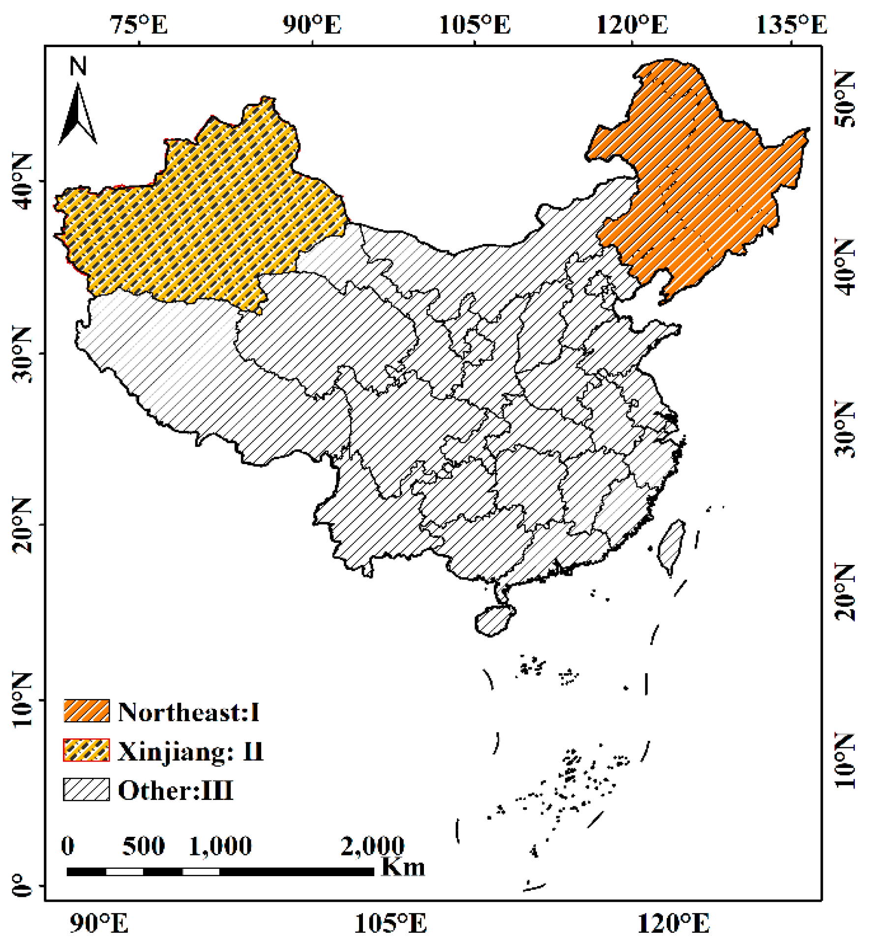
Numerous studies have demonstrated that no single standard algorithm can describe snow cover characteristics well everywhere [19,29,32,45]. Thus, regional algorithms that have been calibrated at a local scale might be capable of providing a reasonable snow depth estimation. Similar studies have been carried out over the years by several scholars [46,47,48]. They divided Chinese snow cover into different regions based on topography, land cover, and snow cover duration, e.g., Xingjiang, Qinghai–Tibetan Plateau, Northeast, and others. Based on these previous studies, China’s snow cover is divided into three regions (Figure 2):
(1) Region I: Northeast China
Northeast China consists of Liaoning, Jilin, Heilongjiang, and eastern Inner Mongolia. Various land cover types are unevenly distributed. Cultivated and forest land predominate in Northeast China, and large uncertainties in snow depth retrieval are associated with forest cover. Foster et al. [14] developed an algorithm that accounts for the influence of forest cover on brightness temperature. Unfortunately, it tends to overestimate snow depth in China, especially in densely forested areas. Therefore, the Foster algorithm can be improved by the use of 1/(1 − ff) to alleviate overestimation. Referring to the study by Kelly et al. [26] performed in 2009, incorporating a weight factor that limits 1/(1 − ff) within reasonable intervals can reduce overestimation. Thus, we modified the Foster algorithm as follows:
where the constant 0.38 is a regression fitting coefficient between AMSR-E brightness temperatures and weather station observations, and 0.7 is the weight factor that keeps the term 1/(1 − ff) within a range of 1 to 5 (Figure 3). For a weight factor value of 0.5 or 0.9, the algorithm still overestimates snow depth in dense forest areas.
SD = 0.38 × (TB19h − TB37h)/(1 − 0.7 × ff),
(2) Region II: Xinjiang
The Xinjiang Uyghur Autonomous Region is located in northwest China. The southern and northern parts of Xinjiang are dominated by grass, and the land cover in the central part is mainly bare ground dominated by desert (Figure 1). Snow cover is relatively thick in northern Xinjiang, where underestimation usually occurs (e.g., by the FY-3B and WESTDC algorithms). Based on scatter diagrams of station snow depth versus satellite BTD from the AMSR-E sensor in the 2002–2009 period (not shown here), the combination of cross-polarization at 19 GHz and 37 GHz was selected. The shorter 37 GHz wavelength emissions from the ground will be scattered more by the snowpack than the longer 19 GHz wavelength emissions. The brightness temperature at vertical polarization is less affected by incidence angle [34]. Moreover, the brightness temperature of cross-polarization is more sensitive to snow depth than that of co-polarization, owing to the effects of depth hoar [15,17,32,37,38,49]. The regression equation is
where the constant 0.48 is a regression fitting coefficient between AMSR-E brightness temperatures and weather station observations. At the bottom of snowpack, the snow has evolved with time and undergone compaction due to the overburden and freeze/melt cycle, which makes grain size larger. Snow grain size increases with layer depth (0.3–3 mm). Especially for the depth hoar, the radius can be larger than 3 mm because of snow metamorphism [19]. Moreover, the temperature brightness gradient for cross-polarization is higher than that for co-polarization because of a better penetration capacity of vertical polarization. These factors explain why the fitting coefficient is 0.48 rather than 1.59 in Chang’s algorithm for which the assumptions fail in Xinjiang.
SD=0.48 × (TB19v − TB37h),
(3) Region III: Others
In areas other than Xinjiang and northeastern China, a mixed-pixel method is suitable because of complex land cover and thin snow cover, and the original FY-3B method performs well at retrieving snow depth from shallow snowpack [17]. Therefore, the FY-3B algorithm was used to estimate snow depth in Region III.
3. Results
The main framework of the paper is to first show the deficiencies and advantages of current empirical algorithms and then develop the FY-3D algorithm, which complements their strengths. Comparisons and validations of five well-known algorithms are shown in Section 3.1. Section 3.2 displays the validation and analysis of the FY-3D algorithm.
3.1. Comparisons and Validations of Five Well-Known Algorithms
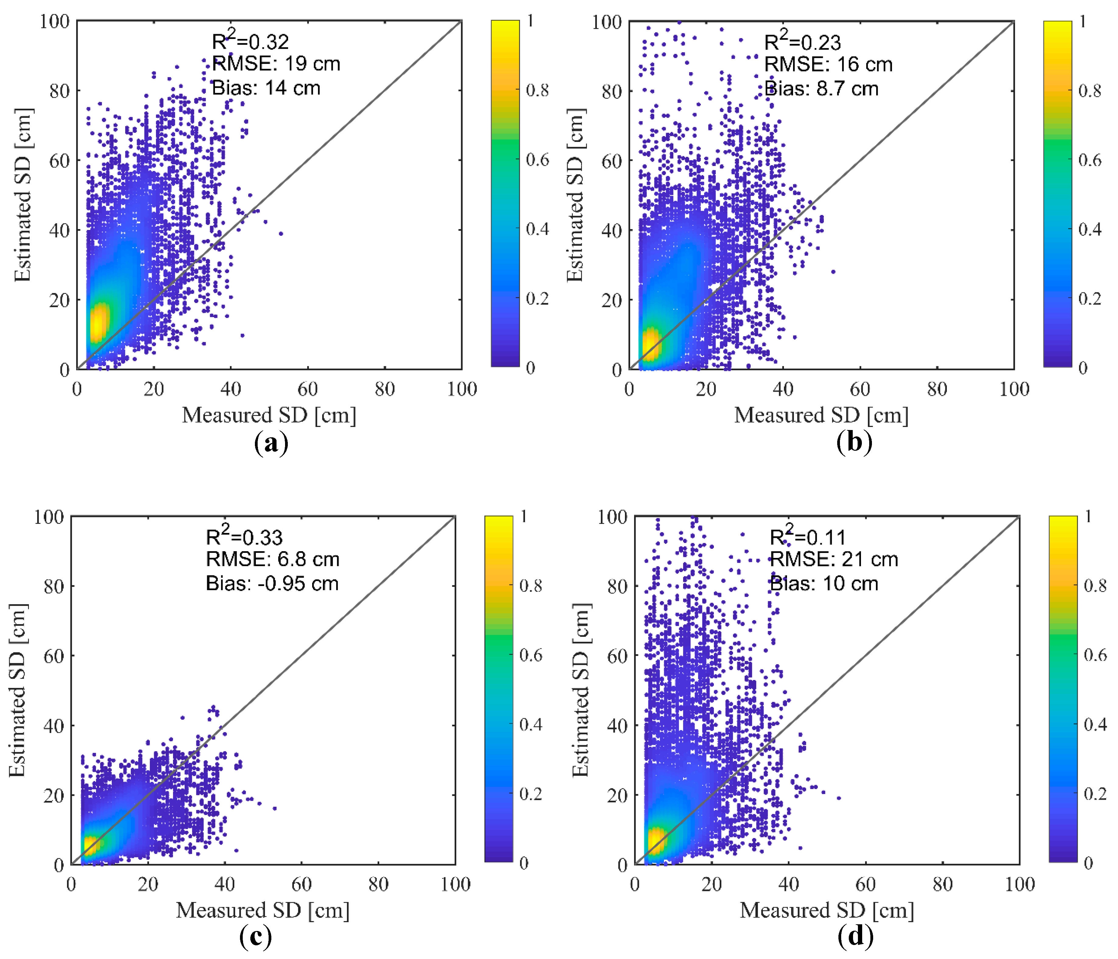
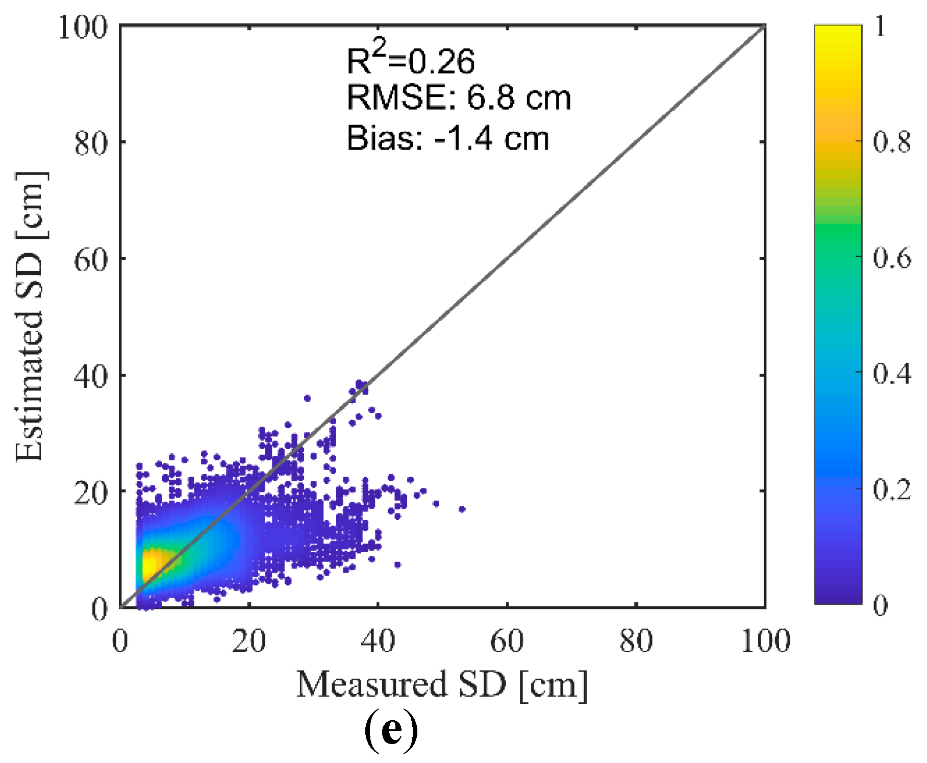
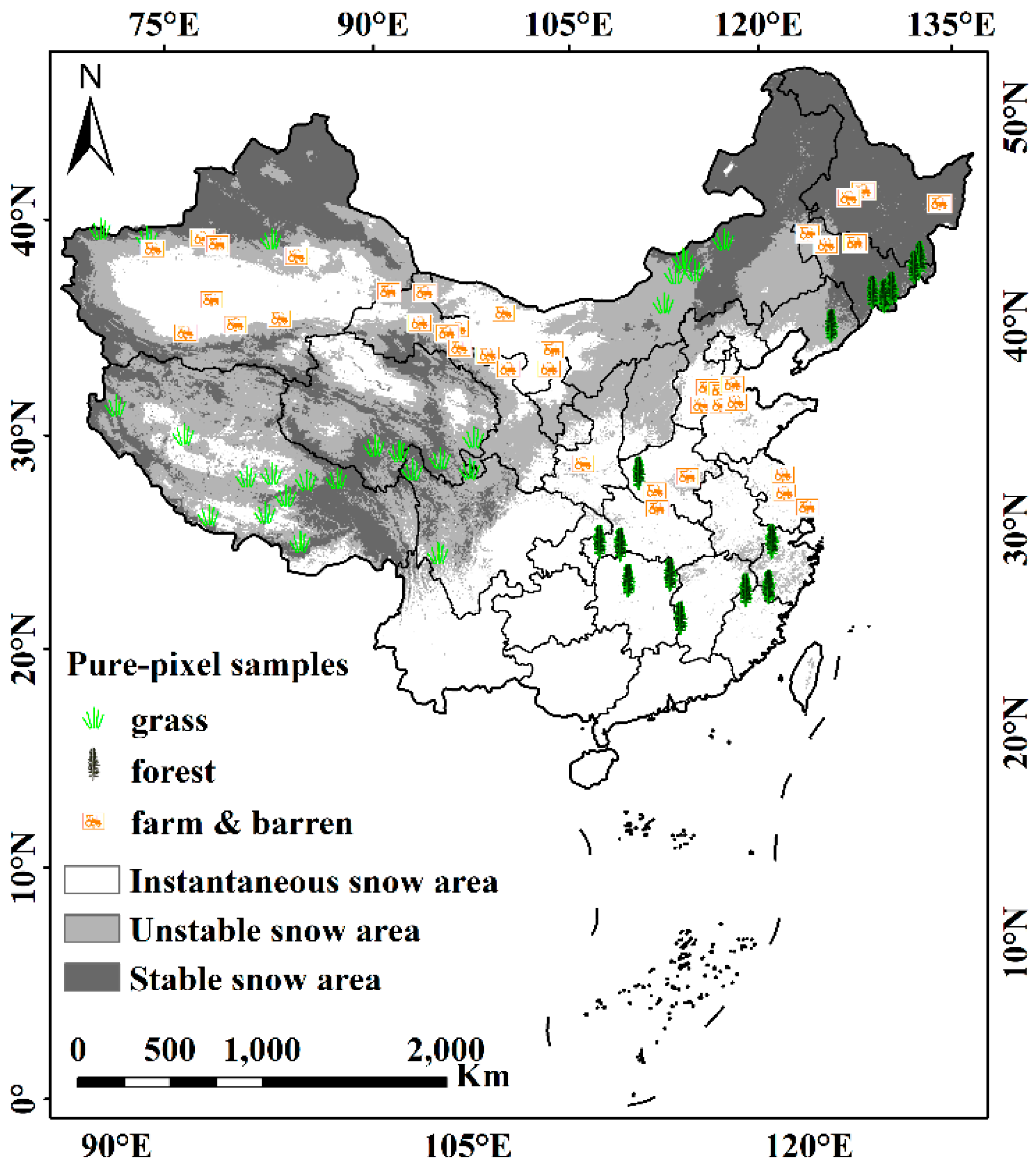
The validation results of five algorithms are shown in Figure 4. The WESTDC and FY-3B algorithms performed better than the other three methods (Figure 4c,e), primarily because they were developed based on Chinese weather station measurements. However, there are still many problems and doubts. For example, the FY-3B version tends to underestimate snow depth for thick snow (greater than 20 cm). The error probably originates from the nonuniform training samples. FY-3B estimates were the sum of values from four individual pure-pixel algorithms, weighted by the land cover fraction. Figure 5 shows the spatial distribution of pure-pixel samples (with a certain land cover fraction greater than 85%), including forest, grass, farm, and barren. The base map is snow types based on snow cover days (instantaneous snow cover: 0–10 days; unstable snow cover: 10–60 days; stable snow cover: 60–365 days). The stable snow cover areas usually are covered with deep snow, such as Xinjiang and Northeast China. As shown in Figure 5, many pure pixels are mainly distributed in thin snow dominated areas, while there are few samples in Northeast China and Xinjiang. Therefore, underestimation occurs for empirical relationships presented in Equation (7).
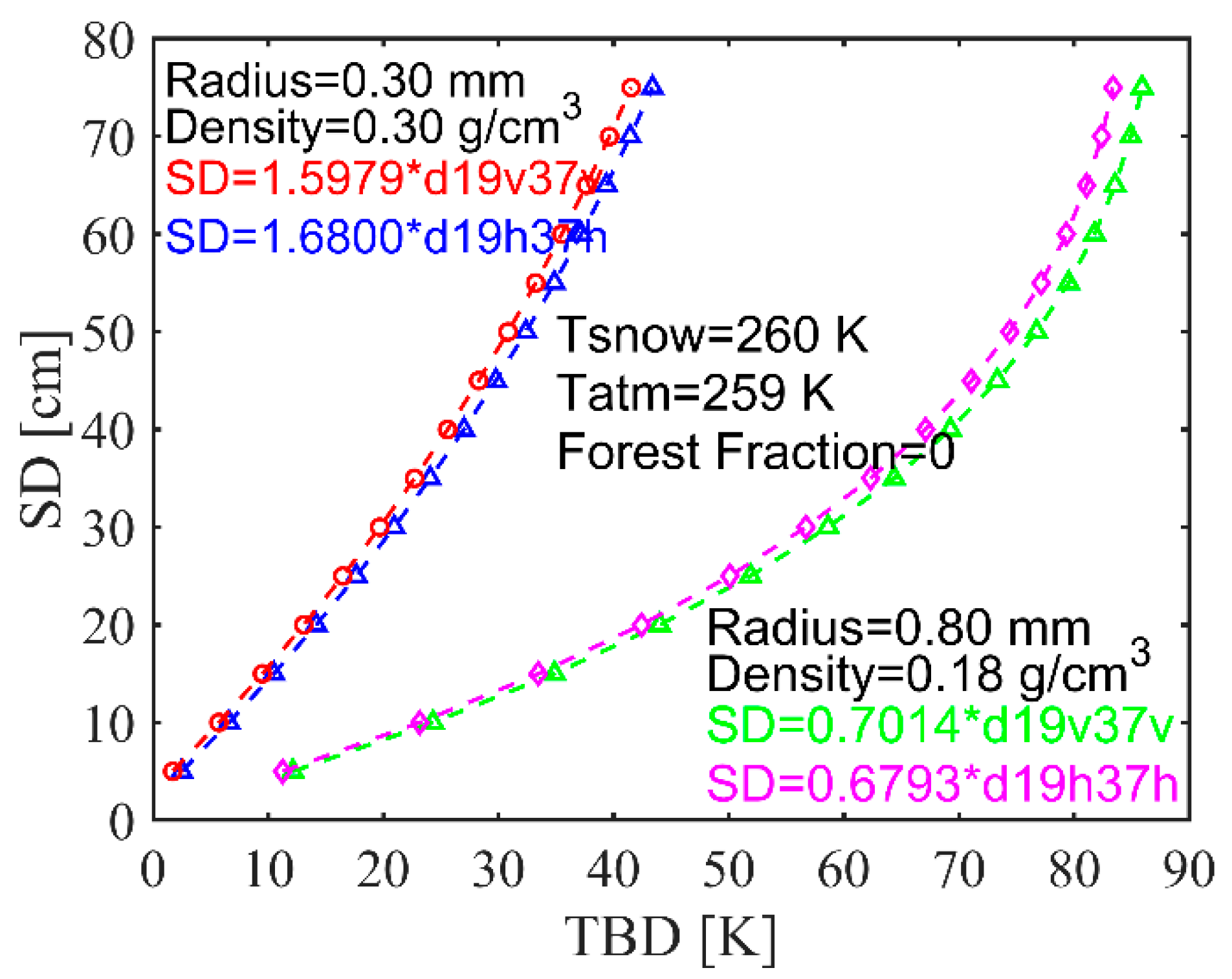
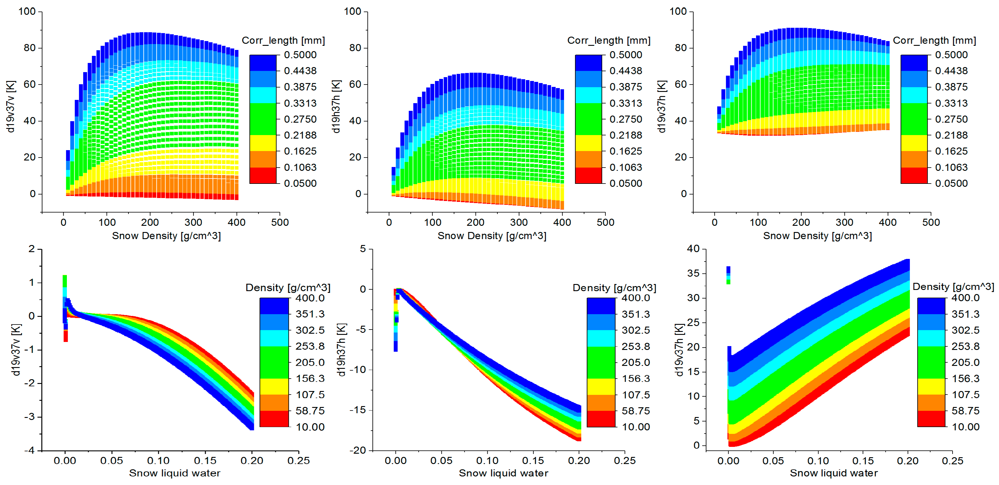
Figure 4b shows that the AMSR-E algorithm generally tends to overestimate snow depth in China compared with ground meteorological station observations. The main cause is that the dynamic coefficient, polarization factor pol36 = Tb36V − Tb36H or pol18 = Tb18V − Tb18H, does not clearly indicate the variation of snow grain size and may need adjustment with further testing [26]. Figure 4a shows that the Chang algorithm produces larger errors of overestimation in China. The fitting coefficient value is 1.59, based on the assumption that the snow density is 0.30 g/cm3 and snow grain size is 0.30 mm. In situ measurements, however, show that these assumptions fail in China. The grain radius of fresh snow in the uppermost layer is approximately 0.30 mm, while the size within the middle or bottom layers is up to 4 mm [37,38]. Figure 6 shows a simulation of the single-layer HUT model with different inputs. The input variables are snow grain radius and snow density, and fixed parameters are snow temperature, atmospheric temperature, and forest fraction. The result shows that the fitting coefficients vary with different inputs. The fitting coefficients are 1.5979 and 1.6800, respectively, for horizontal and vertical polarization under the assumptions of the Chang algorithm (snow density, 0.30 g/cm3; snow grain radius, 0.30 mm). However, the coefficients are 0.7014 and 0.6793, respectively, for a snow density of 0.18 g/cm3 and snow grain radius of 0.80 mm, based on Chinese field work measurements in 2018 (Figure 1 and Figure 7). Figure 4c also shows that the WESTDC algorithm has better performance than Chang’s when the fitting coefficient is 0.66 rather than 1.59.
Figure 4d shows the performance of the Foster algorithm. The coefficient was changed from 1.59 to 0.78. The algorithm also accounts for the tendency of forest cover to reduce the sensitivity of brightness temperature to snow depth. However, it is noteworthy that false high retrievals occur. Owing to the equation form p = 1/(1 − ff) and high fitting coefficient (0.78) in China, the snow depth shows explosive growth when the forest fraction (ff) is greater than 60% (Figure 3, blue line). Thus, the Foster algorithm does not perform well on areas covered by dense forest in China. Figure 3 also shows that a weight factor (a) that limits 1/(1 − ff) within reasonable intervals can reduce overestimation. This study offers a new idea for improving the Foster algorithm.
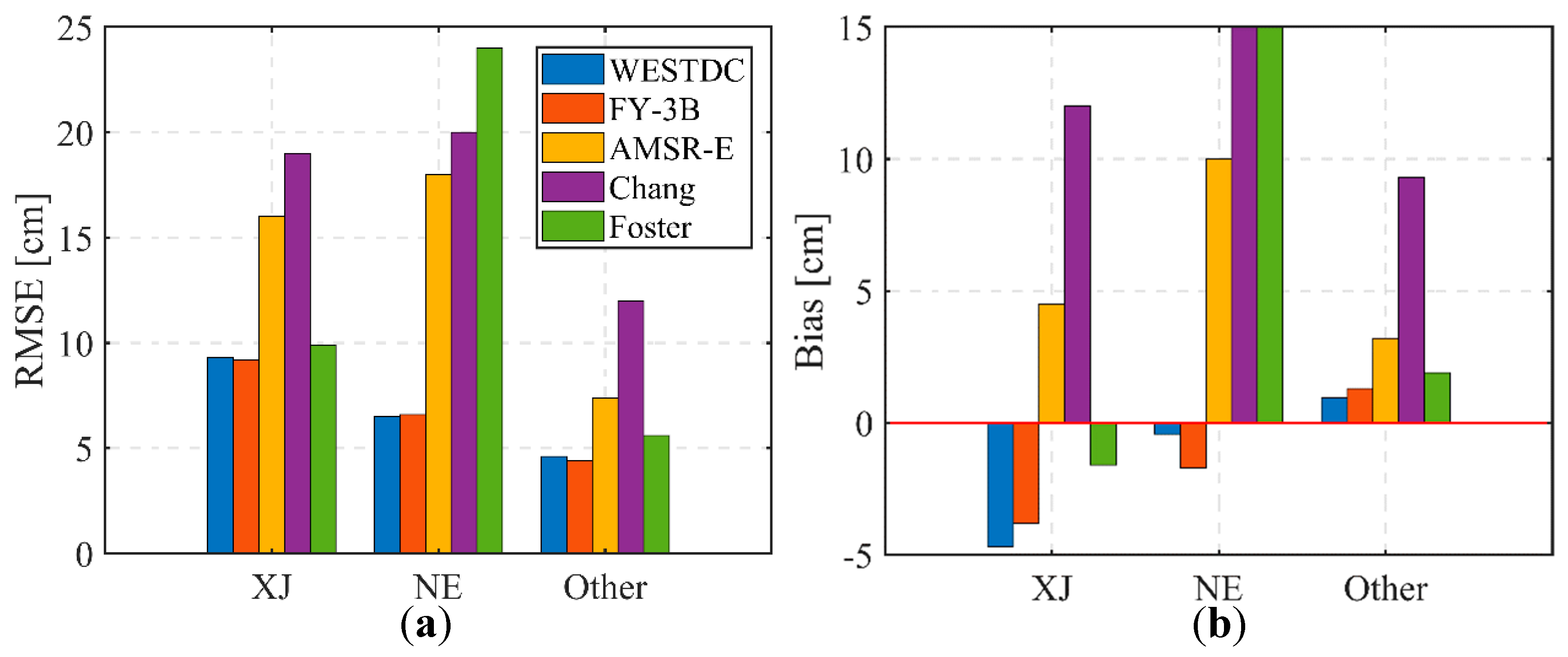
To illustrate the performance of various algorithms in three areas (Xinjiang, Northeast China, and others; Figure 2), the regional validation is shown in Figure 8. The pattern is similar to that of the whole validation (Figure 4). Regardless of location, the WESTDC and FY-3B algorithms perform best based on their root mean square errors (RMSEs). However, they tend to underestimate the snow depth in Xinjiang and Northeast China and overestimate it in other areas. As mentioned earlier, the Foster algorithm performs well in open or sparsely vegetated areas, such as in Xinjiang, where the land cover is mainly barren or grassland. Conversely, it yields the poorest estimates in forested areas, such as Northeastern China. Thus, the five well-known operational snow depth retrieval algorithms cannot fully capture the temporal and spatial distribution of snow cover in China. It is essential to develop a suite of algorithms based on China’s snow cover characteristics, rather than directly implement FY-3B/MWRI’s operational empirical retrieval algorithm.
3.2. Validation and Analysis of FY-3D Algorithm
Section 2.2 presents the FY-3D algorithm. In this paper, the snow depth product retrieved using the FY-3D algorithm is validated rather than the algorithms because the product’s performance without any auxiliary data is what we are interested in. To mitigate any distinct borders in retrievals between adjacent pixels from different regions, a moving-average filter was used to perform smoothing. To demonstrate the performance of the FY-3D algorithm, three products retrieved from the FY-3B, WESTDC, and FY-3D algorithms were validated and compared.
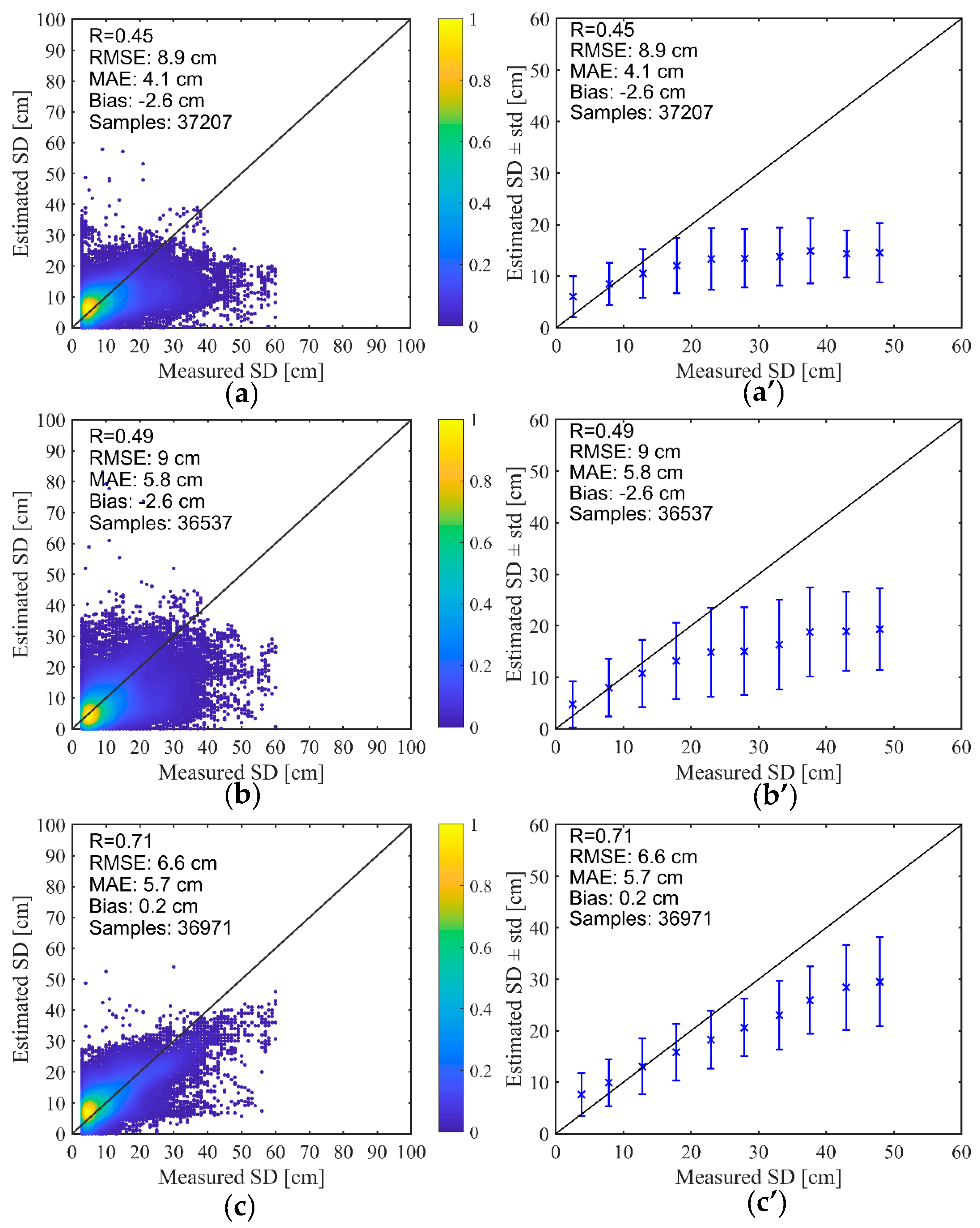
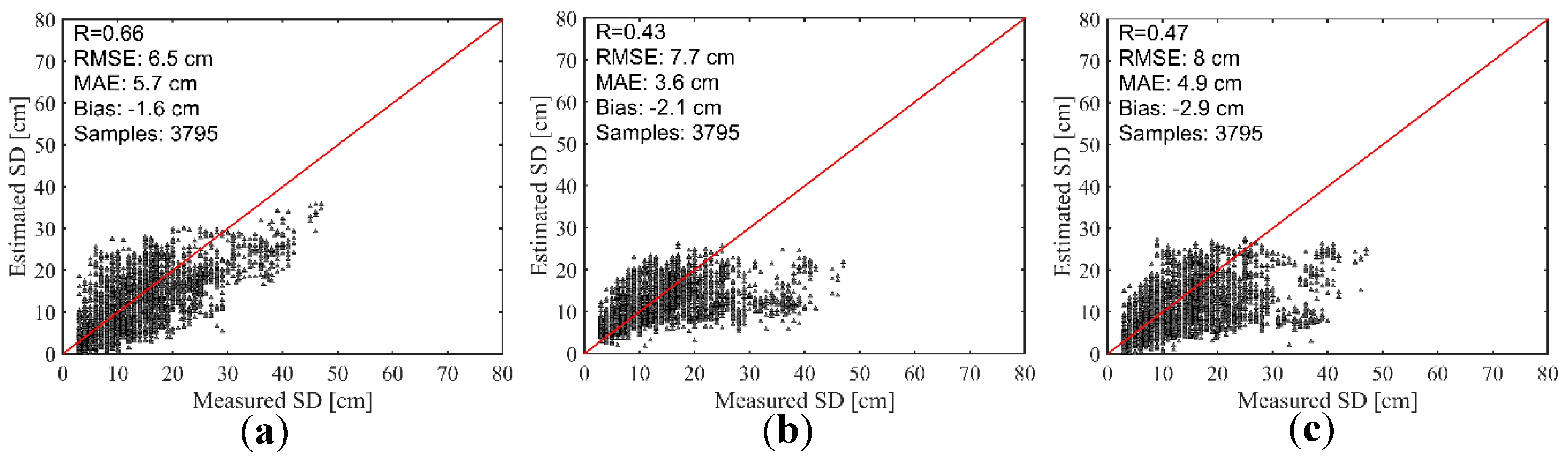
As shown in Figure 9, the FY-3D algorithm’s RMSE and bias are 6.6 cm and 0.2 cm, respectively. The correlation coefficient is 0.71, which is greater than those of the other algorithms. The RMSEs of the products retrieved with the WESTDC and original FY-3B algorithms are 8.9 cm and 9.0 cm, respectively. The WESTDC and original FY-3B algorithms encounter underestimation at snowpack deeper than 13 cm. The bias of the WESTDC and original FY-3B algorithms is −2.6 cm, while it is just 0.2 cm for the FY-3D algorithm, which also shows that the FY-3D algorithm performs better than the others. Owing to limited FY-3D/MWRI data (1 January to 31 March 2018), there are only about 3800 samples to validate the new algorithm. Figure 10 shows that snow depths estimated with FY-3D brightness temperature are closer to the ground truth.
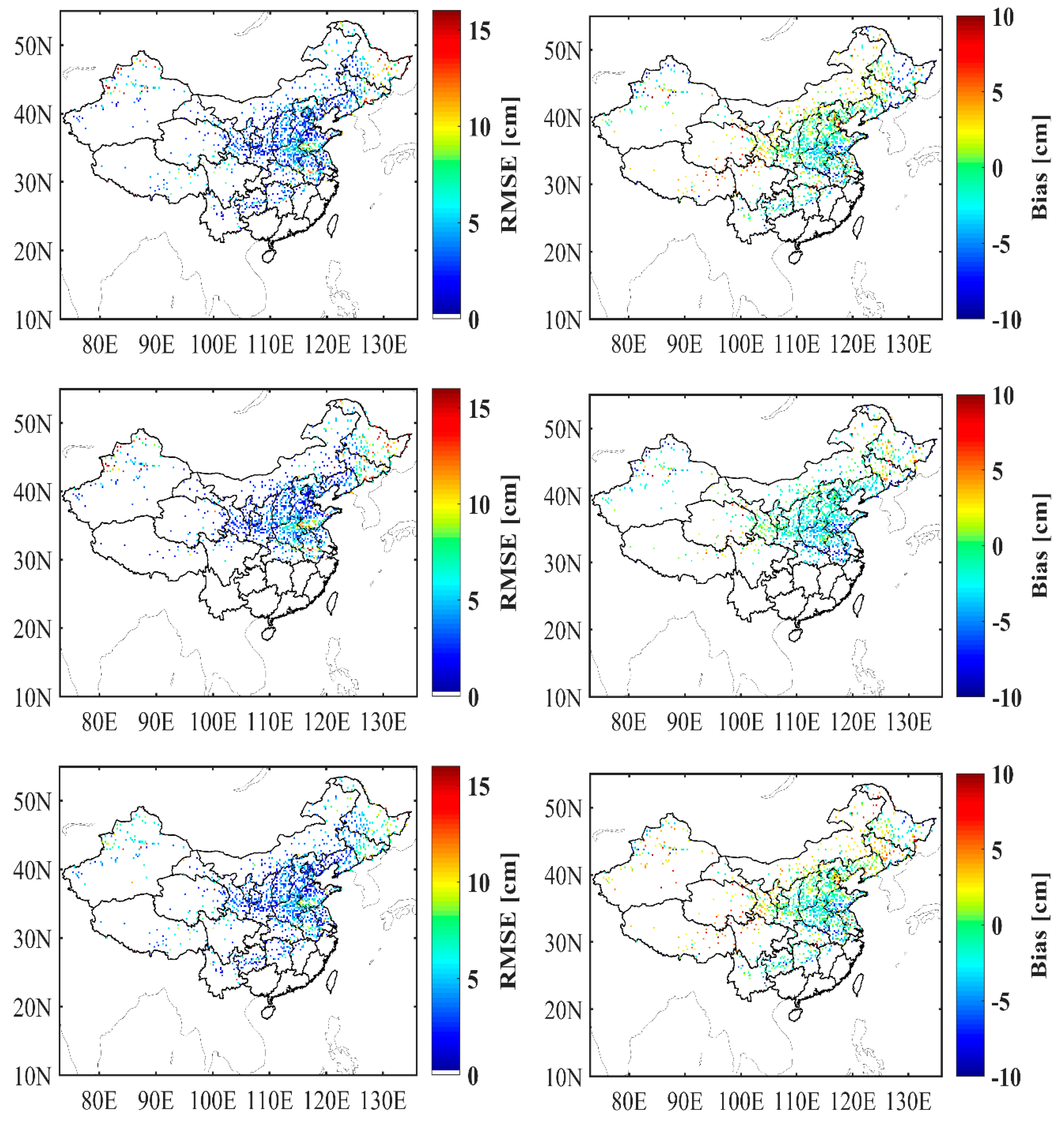
Figure 11 shows the spatial distribution of RMSE and bias of pixels where the sites are located. The RMSE distribution indicates that the three algorithms perform similarly in Region III. However, there are large differences in Xinjiang and Northeast China. The FY-3D algorithm has an advantage over the others in northern Xinjiang and Heilongjiang Provinces because of low RMSEs. The results also confirm that the FY-3D algorithm is more sensitive to deep snow. In terms of bias (difference between retrieved and measured snow depth), Figure 11 shows that underestimation occurs mostly in the North China Plain and South China, where the snow is often thin and wet. Wet snow usually corresponds to low BTD, resulting in underestimation [32,45,50]. In northern Xinjiang and Northeast China, the original FY-3B algorithm produces the lowest bias, as low as −10 cm. The WESTDC algorithm performs better than the original FY-3B algorithm in deep snow cover, as shown in Figure 11. Interestingly, there is overestimation in the Qinghai–Tibetan Plateau. There, the snow cover differs from that in other seasonally snow-covered regions; it is often shallow, patchy, and of short duration [50,51,52]. A distinct meteorological characteristic is the large diurnal temperature range, which causes snow to undergo frequent freeze–thaw cycles. Note that these cycles lead to rapid grain growth and consequently to a low brightness temperature [45,50]. Frozen soil is also a factor that reduces the accuracy of estimates in the Qinghai–Tibetan Plateau. Both snow and frozen ground are volume-scattering materials, and they have similar microwave radiation characteristics, making them difficult to distinguish.
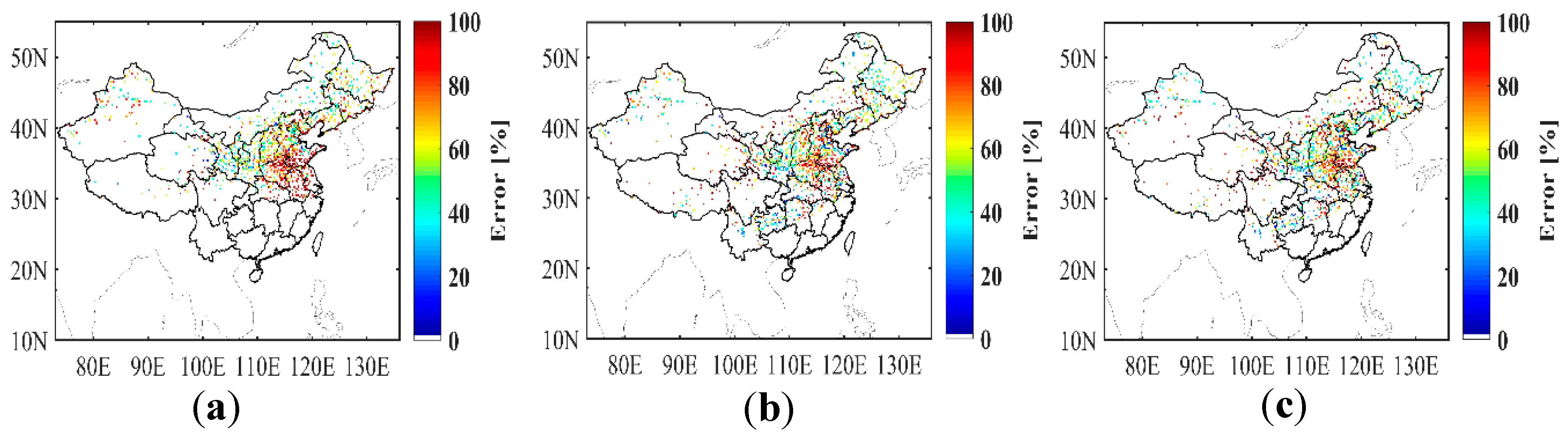
In view of the heterogeneity of snow depth in the three regions, RMSE and bias cannot fully explain where an algorithm consistently performs well or poorly. Thus, the spatial distribution of relative error (RMSE divided by mean snow depth) is shown in Figure 12. First, the error in areas of shallow snow cover is higher than that in thick snow areas. This pattern is caused by the different mean snow depth. Similarly, a high RMSE does not mean poor performance. What is certain, however, is that the FY-3D algorithm performs best in Xinjiang and the northeast regardless of RMSE, bias, or error.
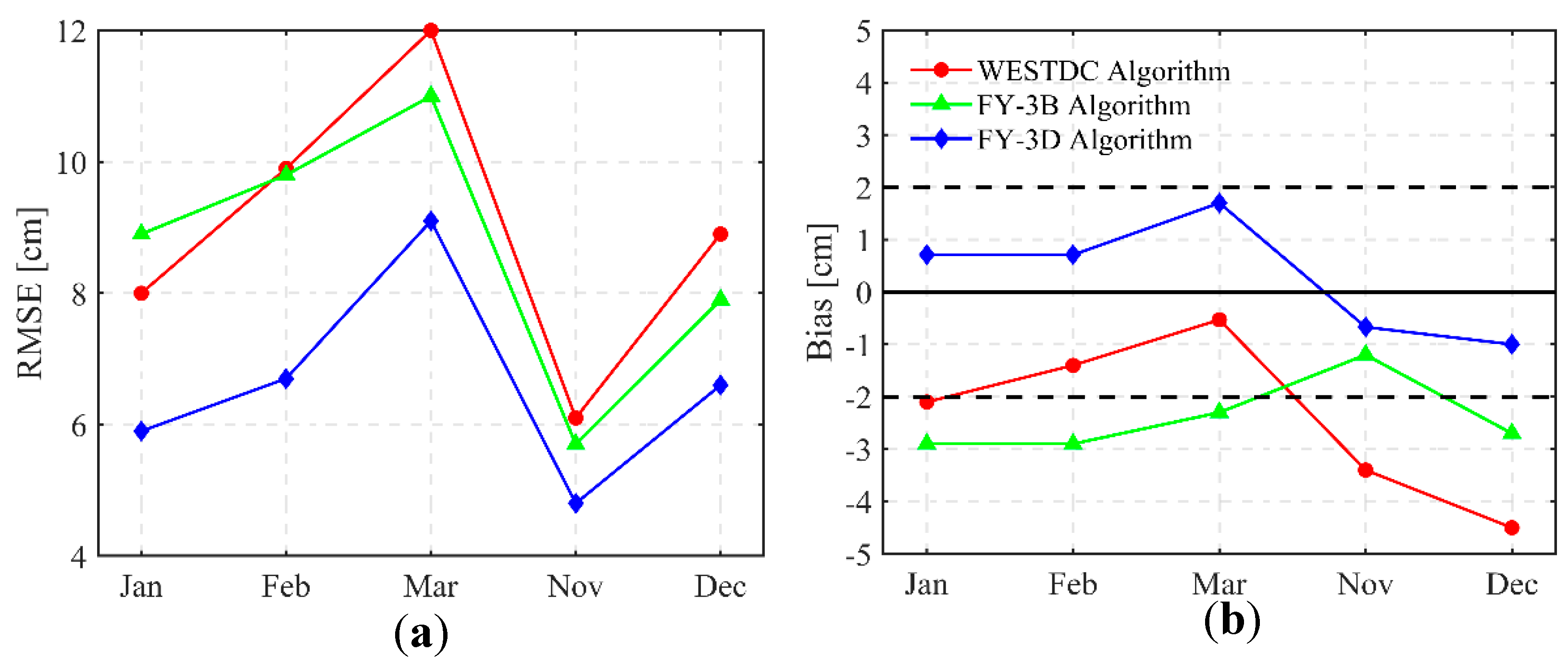
To evaluate the monthly performance of the algorithms, RMSE and bias were calculated independently. The results are shown in Figure 13. The maximal RMSE occurs in March. This poor performance is associated with the confounding effect of snow grain size and stratigraphy. Another reason is thick snow cover. The minimum RMSE occurs in November. On the one hand, the snow parameters are stable and have no evolution. Therefore, the relationship between snow depth and brightness temperature is relatively strong. On the other hand, the snow cover is shallow in November. Bias ranges from −1 to 2 for the FY-3D algorithm, and it performs better in the snowy season, except in March.
4. Discussion
4.1. Influence of Snow Microphysical Properties
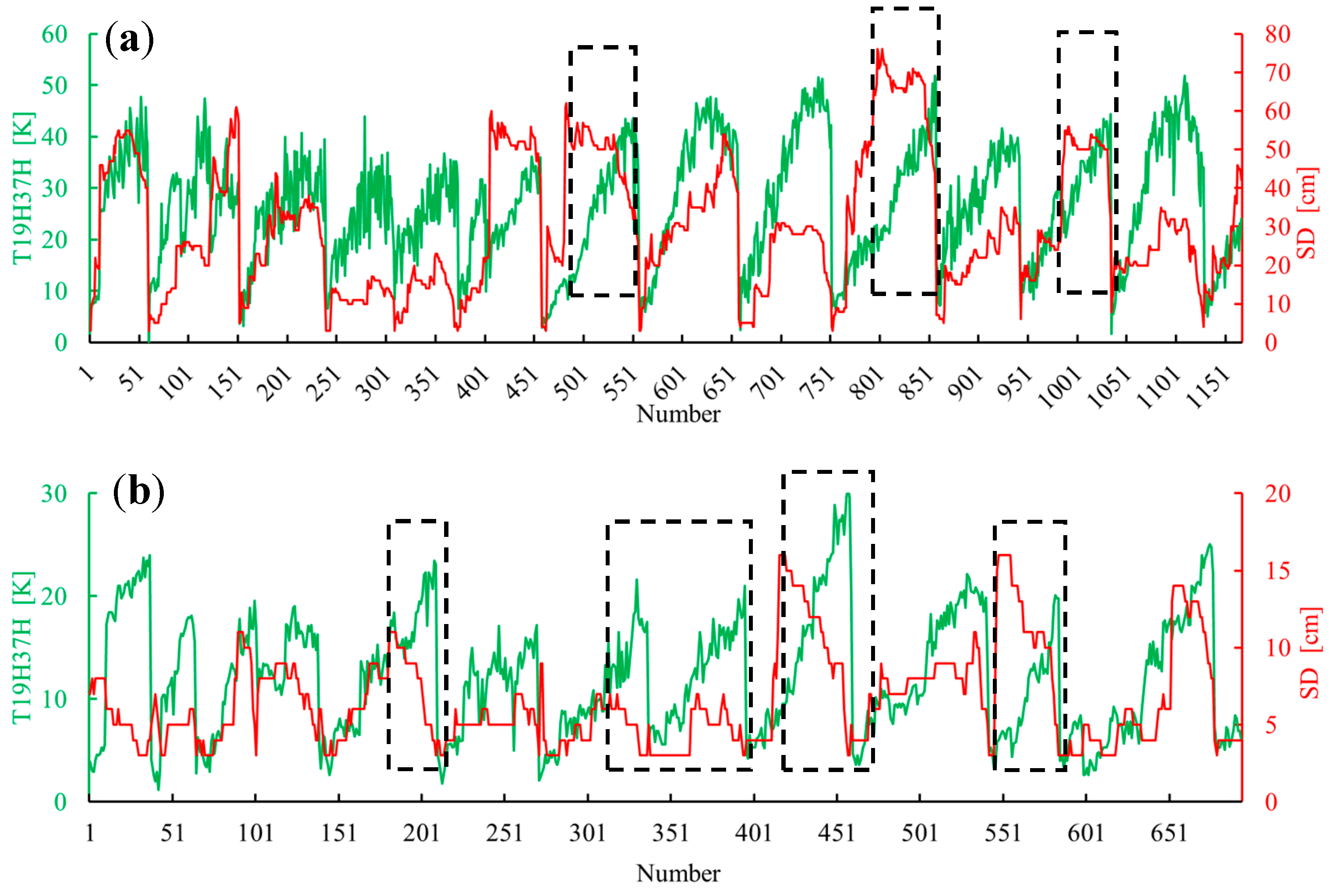
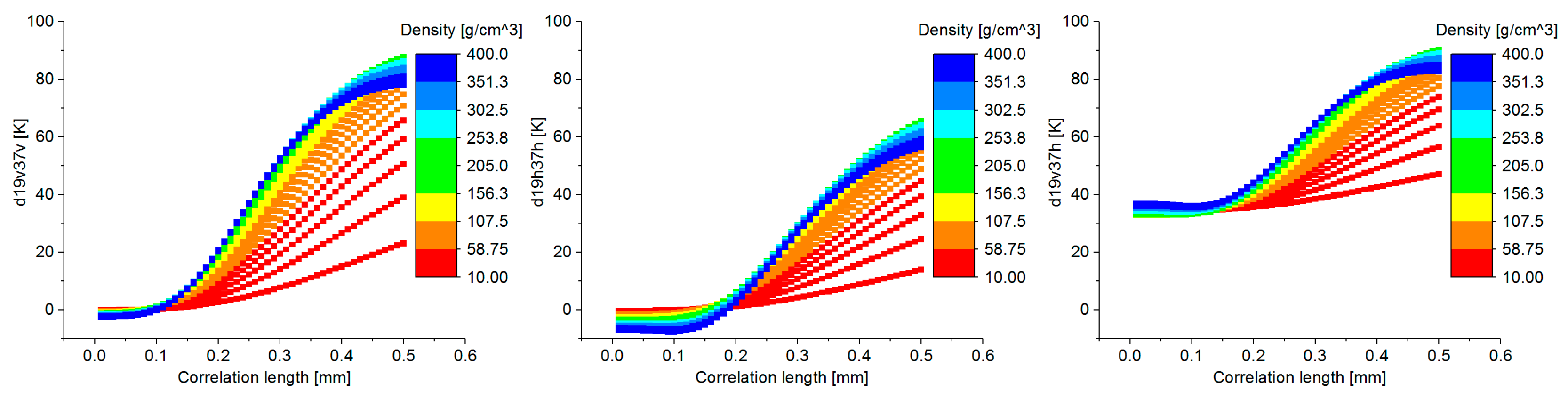
PMW retrievals are plagued by a number of challenges, which often disrupt the relationship between snow depth and brightness temperature, resulting in poor estimation [34,38,45,53,54]. Neglecting to account for snow’s microphysical properties (mostly grain size and density) tends to cause retrieval errors. Figure 14 shows time series of snow depth (station observations, 2002–2009) and TBD (19 GHz and 37 GHz, AMSR-E, 2002–2009) at Aletai station (deep snow, maximum snow depth 57 cm, mean snow depth 26 cm) and Mingshui station (thin snow, maximum snow depth 23 cm, mean snow depth 10 cm). When the snow depth is invariable, however, the TBD still increases at Aletai station, as shown within the dashed black frames in Figure 14a. Figure 14b shows that the TBD increases with decreasing snow depth at Mingshui station. Simulation with the single-layer microwave emission model of layered snowpack (MEMLS) model shows that the TBD increases with increasing snow grain correlation length (Figure 15, top) and snow density (Figure 15, middle) and decreases with increasing humidity except for cross-polarization (Figure 15, bottom). TBD for cross-polarization (TB19v − TB37h) increases with increased snow liquid water content. This is mainly because the cross-polarization difference at 37 GHz (TB37v − TB37h) is large due to water dielectric properties, and (TB19v − TB37h) can be expressed as (TB19v − TB37v) + (TB37v − TB37h). It is clear that (TB19v − TB37v) is small (Figure 15, bottom left), so the major contributions are from (TB37v − TB37h). Therefore, the factor that can be used to explain the anomalous pattern in Figure 14 is the evolution in snow grain size and snow density. Although empirical and physical models have been developed to predict the growth of snow crystals and increase in density [25,26], they are not suited to regional- or global-scale conditions.
4.2. Influence of Snow Density on SWE Mapping
Snow density is a key parameter that not only confounds the relationship between TB and snow depth, but also influences SWE [17,32,33]. Much SWE retrieval processing is based on snow depth information
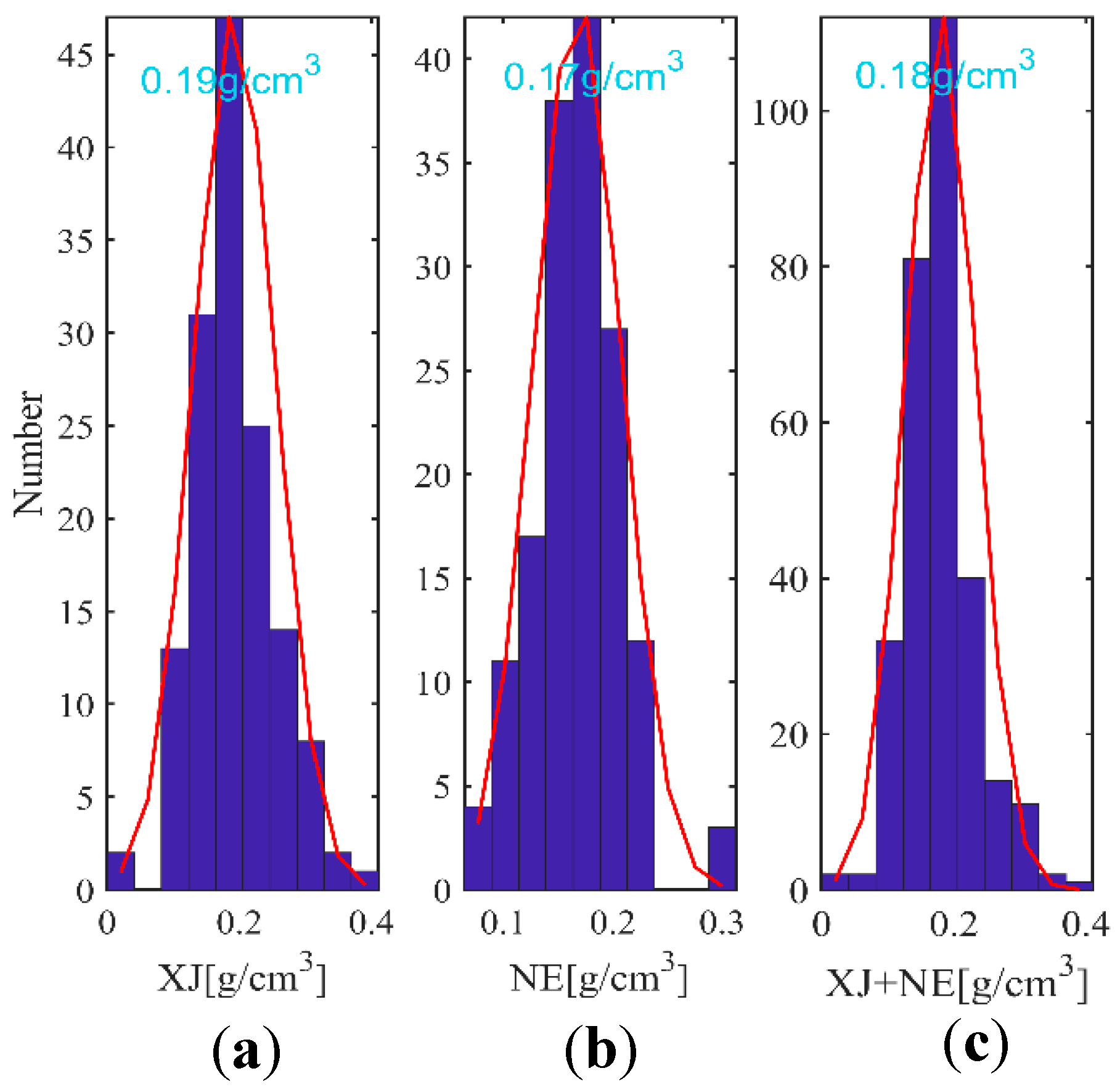
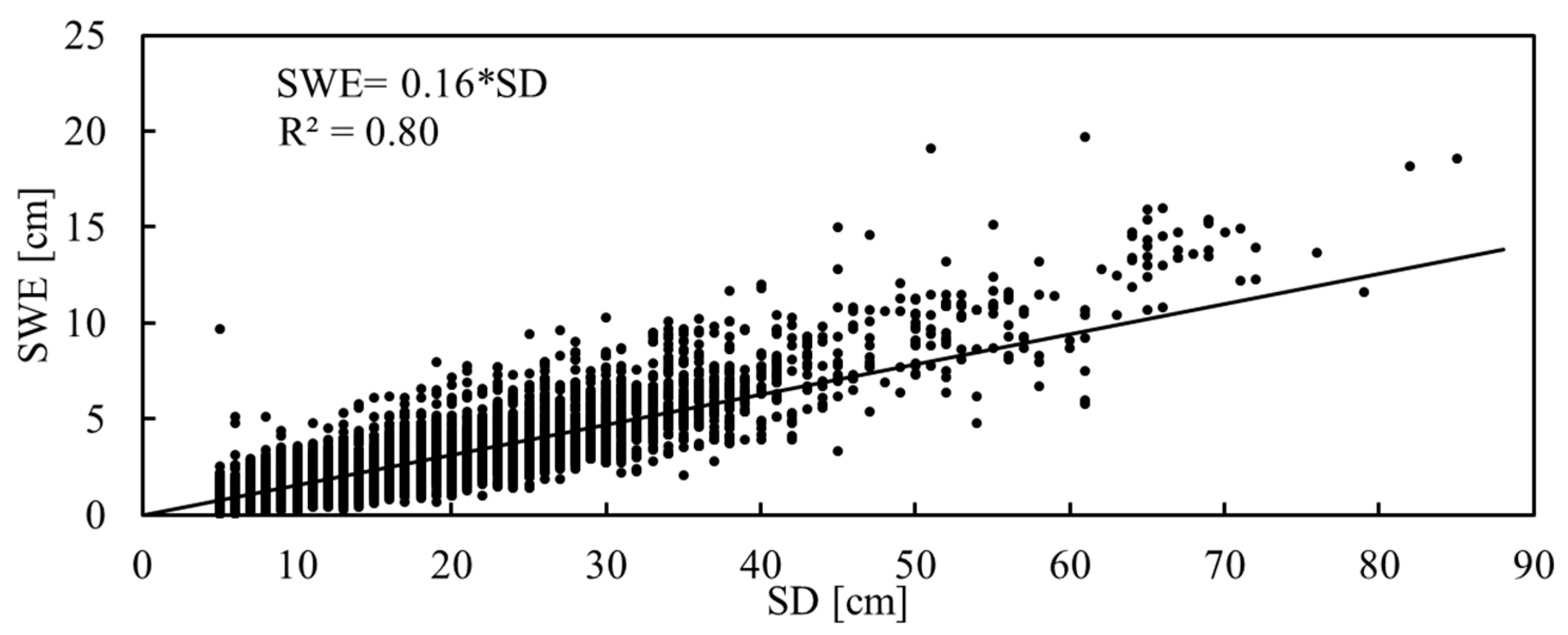
where SD is the snow depth (cm), ρs is the snow density (g/cm3), ρw is the density of water (1 g/cm3), and SWE is measured in millimeters of water. The first implementation of the FY-3B SWE retrieval scheme utilized reference snow density of Sturm’s climatological snow classes [55,56]. Based on in situ snow course data in Xinjiang and Northeast China, however, the snow density is generally around 0.18 g/cm3 (Table 2, Figure 7). The average snow densities in the northeast and Xinjiang are similar, 0.19 g/cm3 and 0.17 g/cm3, respectively. Weather station observations from 1992 to 2009 include snow pressure, which can be converted to SWE. The relationship between snow depth and SWE is shown in Figure 16. The slope of the fitting is 0.16, meaning that snow density is about 0.16 g/cm3.
SWE = SD × ρs/ρw × 10,
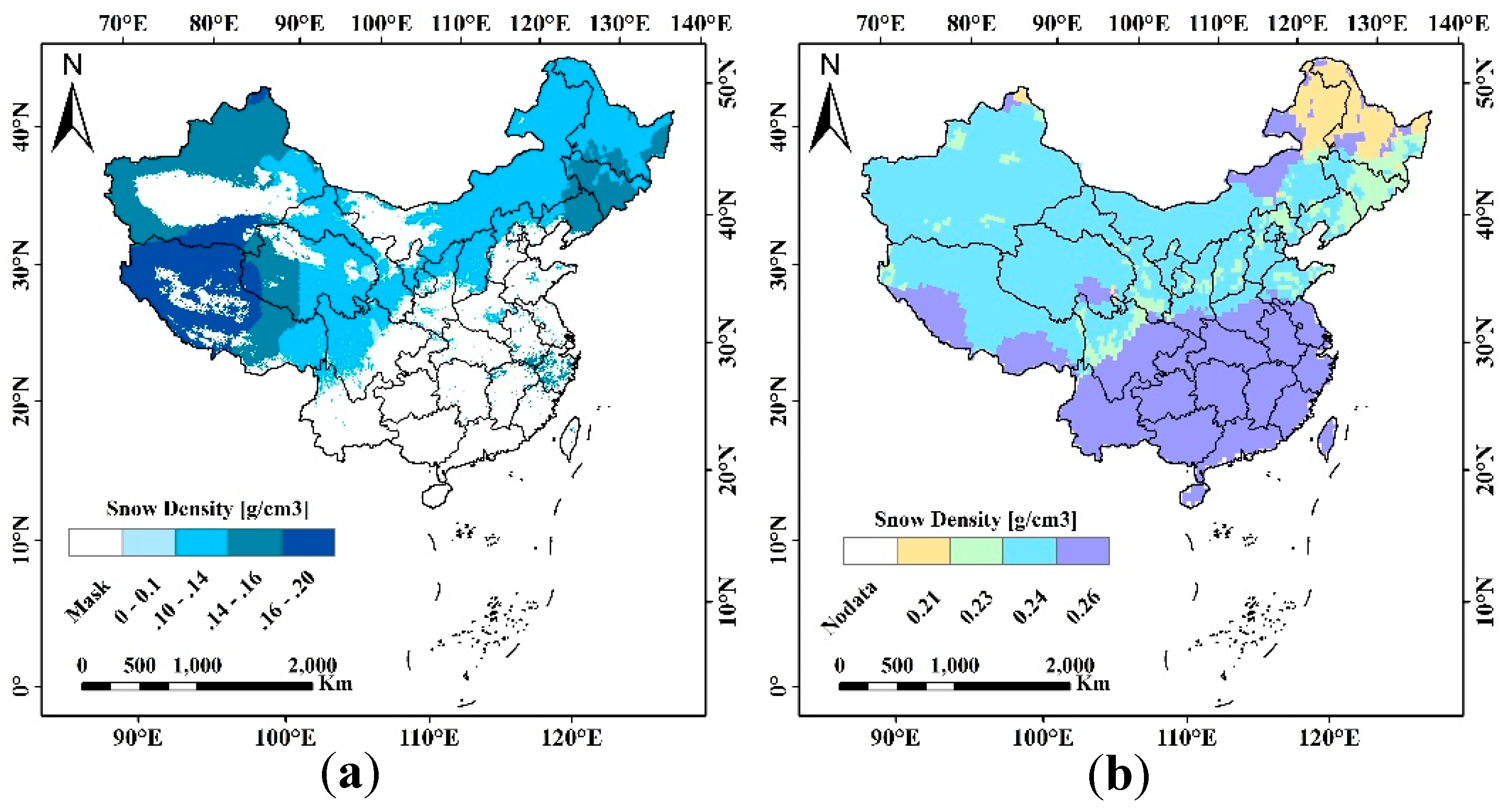
Figure 17a is a Kriging interpolation map of snow densities obtained from weather stations during the winters of 2002–2009. It is masked with instantaneous snow cover in Figure 5. Figure 17b shows the spatial distribution of snow density based on Sturm’s climatological snow classes [55,56]. It is clear that snow density based on Sturm’s climatological snow classes (minimum ~ 0.21) tends to be bigger than that in China (maximum ~ 0.20), which results in systematic overestimation of SWE. Therefore, the snow density used in the FY-3D SWE version is 0.18 g/cm3 rather than that in the Kriging interpolation because of uncertainties resulting from unevenly distributed weather stations (Figure 1). In future work, the temporospatial distribution of snow density in China will be mapped based on field measurements from 2018 to 2021 and weather station observations.
4.3. Influence of Forest Cover Fraction
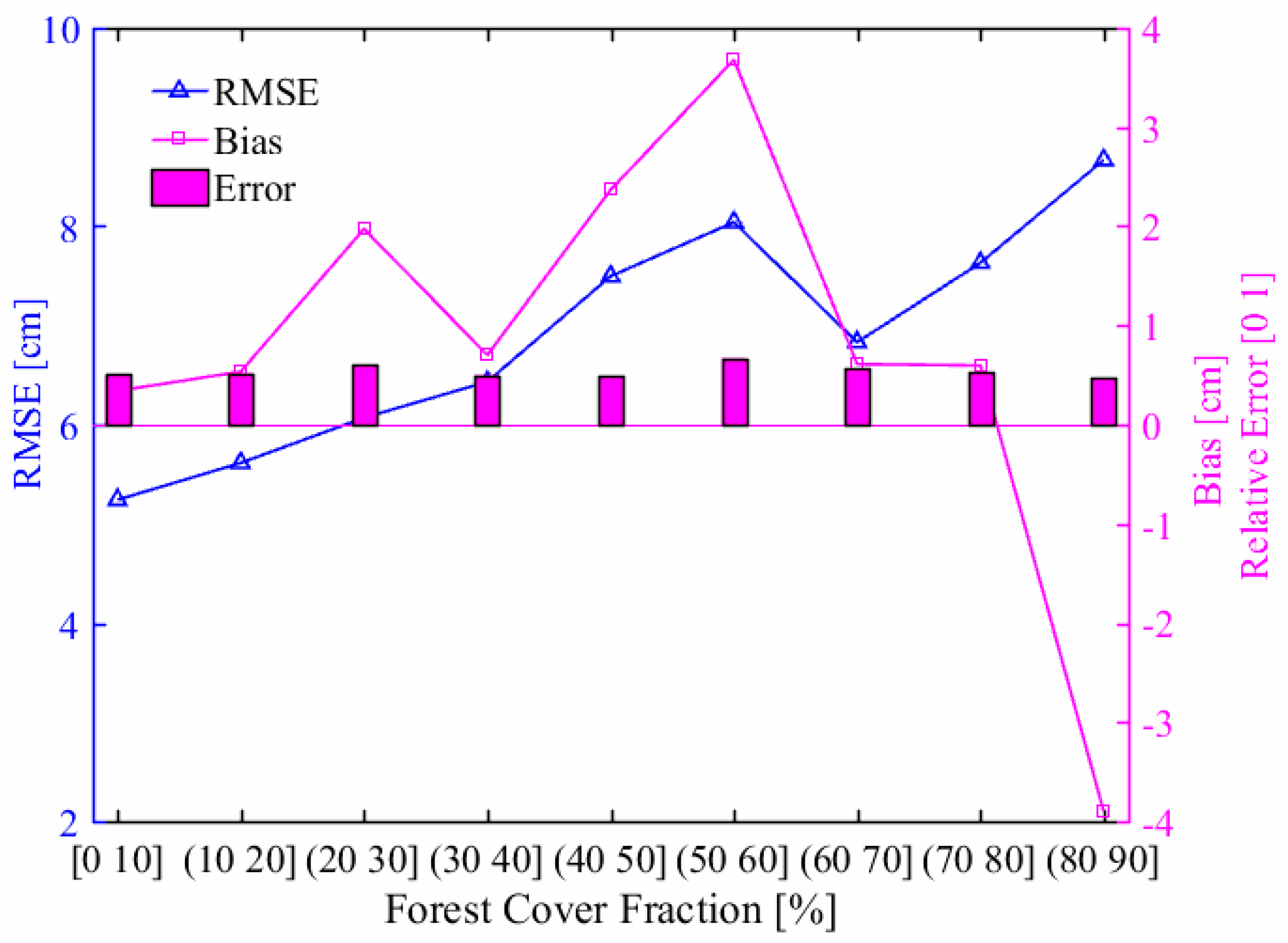
Forest cover represents a significant source of error in satellite PMW snow depth and SWE retrieval algorithms. In this work, we improved the Foster algorithm by employing a weight factor to avoid overestimation in densely forested areas. In fact, this method results in overestimation in sparsely forested areas. Figure 18 shows that RMSE increases with increasing forest cover fraction, and bias overestimation is serious as forest fractions range from 20% to 60% (Figure 18, magenta line), mainly caused by mixed pixels [38]. When the forest fraction is greater than 80%, serious underestimation occurs because of minimal penetration depth of the microwave signal in the forest canopy. Because snow depth varies in different areas, relative error is more reasonable to show the algorithm’s performance. Although RMSEs in densely forested areas are large, relative errors are still smooth, not larger than those in sparsely forested areas. In future work, we will study the influence of forest on brightness temperature with a physically based radiative transfer model and the influence of snow microphysical properties on brightness temperature with a snow forward model, then calibrate microwave signals to improve snow depth estimation [53,54].
5. Conclusions
In this study, the performance of five snow depth estimation methods was evaluated using in situ snow depth measurements and satellite brightness temperatures. The results show that the WESTDC and FY-3B algorithms performed well. However, there was persistent underestimation in thick snow cover (greater than 20 cm). The purpose of the study was to develop a new algorithm that can solve the problem of underestimation of deep snow. Ideally, it should be possible to retrieve deep and shallow snow depths, as the AMSR-E algorithm does. However, PMW remote sensing still cannot distinguish deep snow from thin snow and only can detect snow cover, i.e., snow vs. snow-free. Thus, establishing regional algorithms calibrated at a local scale is a promising approach and may improve snow depth estimation. Thus, we developed regional algorithms for Xinjiang, Northeast China, and other areas. Based on our evaluation and analysis, the FY-3D algorithm performed better than other algorithms. The RMSE and bias were 6.6 cm and 0.2 cm, respectively. Based on an in-situ snow density of 0.18 g/cm3, the RMSE of the SWE is approximately 12 mm.
Author Contributions
L.J. and S.W. conceived and designed the study; S.W. provided the FY-3C/MWRI data and contributed the analysis; J.Y. analyzed the data and wrote the paper; and G.W., J.W. and X.L. contributed analytical tools and methods.
Funding
This research was funded by the Science and Technology Basic Resources Investigation Program of China [2017FY100502] and the National Natural Science Foundation of China [41671334].
Acknowledgments
The authors would like to thank the China Meteorological Administration, National Geomatics Center of China, and National Snow and Ice Data Center for providing land-cover products and satellite data. We would also like to thank the Chinese snow survey teams for providing in situ data. We would like to thank the three anonymous reviewers for their helpful comments.
Conflicts of Interest
The authors declare no conflict of interest.
References
- Fernandes, R.; Zhao, H.; Wang, X.; Key, J.; Qu, X.; Hall, A. Controls on Northern Hemisphere snow albedo feedback quantified using satellite Earth observations. Geophys. Res. Lett. 2009, 36. [Google Scholar] [CrossRef] [Green Version]
- Hernández-Henríquez, M.A.; Déry, S.J.; Derksen, C. Polar amplification and elevation-dependence in trends of Northern Hemisphere snow cover extent, 1971–2014. Environ. Res. Lett. 2015, 10, 044010. [Google Scholar] [CrossRef] [Green Version]
- Derksen, C.; Brown, R. Spring snow cover extent reductions in the 2008–2012 period exceeding climate model projections. Geophys. Res. Lett. 2012, 39. [Google Scholar] [CrossRef]
- Safavi, H.R.; Sajjadi, S.M.; Raghibi, V. Assessment of climate change impacts on climate variables using probabilistic ensemble modeling and trend analysis. Theor. Appl. Climatol. 2017, 130, 635–653. [Google Scholar] [CrossRef]
- De Rosnay, P.; Balsamo, G.; Albergel, C.; Muñoz-Sabater, J.; Isaksen, L. Initialisation of land surface variables for numerical weather prediction. Surv. Geophys. 2014, 35, 607–621. [Google Scholar] [CrossRef]
- Bell, V.A.; Kay, A.L.; Davies, H.N.; Jones, R.G. An assessment of the possible impacts of climate change on snow and peak river flows across Britain. Clim. Chang. 2016, 136, 539–553. [Google Scholar] [CrossRef] [Green Version]
- Barnett, T.P.; Adam, J.C.; Lettenmaier, D.P. Potential impacts of a warming climate on water availability in snow-dominated regions. Nature 2005, 438, 303–309. [Google Scholar] [CrossRef]
- Dressler, K.A.; Leavesley, G.H.; Bales, R.C.; Fassnacht, S.R. Evaluation of gridded snow water equivalent and satellite snow cover products for mountain basins in a hydrologic model. Hydrol. Process. 2006, 20, 673–688. [Google Scholar] [CrossRef]
- Gong, G.; Cohen, J.; Entekhabi, D.; Ge, Y. Hemispheric-scale climate response to Northern Eurasia land surface characteristics and snow anomalies. Glob. Planet. Chang. 2007, 56, 359–370. [Google Scholar] [CrossRef]
- Lemmetyinen, J.; Schwank, M.; Rautiainen, K.; Kontu, A.; Parkkinen, T.; Mätzler, C.; Wiesmann, A.; Wegmüller, U.; Derksen, C.; Toose, P.; et al. Snow density and ground permittivity retrieved from L-band radiometry: Application to experimental data. Remote Sens. Environ. 2016, 180, 377–391. [Google Scholar] [CrossRef]
- Zheng, X.; Li, X.; Jiang, T.; Ding, Y.; Wu, L.; Zhang, S.; Zhao, K. Retrieving soil surface temperature under snowpack using special sensor microwave/imager brightness temperature in forested areas of Heilongjiang, China: An improved method. J. Appl. Remote Sens. 2016, 10, 26016. [Google Scholar] [CrossRef]
- Rautiainen, K.; Lemmetyinen, J.; Schwank, M.; Kontu, A.; Ménard, C.B.; Mätzler, C.; Drusch, M.; Wiesmann, A.; Ikonen, J.; Pulliainen, J. Detection of soil freezing from L-band passive microwave observations. Remote Sens. Environ. 2014, 147, 206–218. [Google Scholar] [CrossRef]
- Chang, A.T.C.; Foster, J.L.; Hall, D.K. Nimbus-7 SMMR derived global snow cover parameters. Ann. Glaciol. 1987, 9, 39–44. [Google Scholar] [CrossRef]
- Foster, J.L.; Chang, A.T.C.; Hall, D.K. Comparison of snow mass estimates from a prototype passive microwave snow algorithm, a revised algorithm and a snow depth climatology. Remote Sens. Environ. 1997, 62, 132–142. [Google Scholar] [CrossRef]
- Derksen, C.; Walker, A.; Goodison, B. Evaluation of passive microwave snow water equivalent retrievals across the boreal forest/tundra transition of western Canada. Remote Sens. Environ. 2005, 96, 315–327. [Google Scholar] [CrossRef]
- Che, T.; Li, X.; Jin, R.; Armstrong, R.; Zhang, T. Snow depth derived from passive microwave remote-sensing data in China. Ann. Glaciol. 2008, 49, 145–154. [Google Scholar] [CrossRef] [Green Version]
- Jiang, L.; Wang, P.; Zhang, L.; Yang, H.; Yang, J. Improvement of snow depth retrieval for FY3B-MWRI in China. Sci. China Earth Sci. 2014, 44, 531–547. [Google Scholar] [CrossRef]
- Santi, E.; Paloscia, S.; Pampaloni, P.; Pettinato, S.; Brogioni, M.; Xiong, C.; Crepaz, A. Analysis of Microwave Emission and Related Indices Over Snow using Experimental Data and a Multilayer Electromagnetic Model. IEEE Trans. Geosci. Remote Sens. 2017, 55, 2097–2110. [Google Scholar] [CrossRef]
- Cai, S.; Li, D.; Durand, M.; Margulis, S.A. Examination of the impacts of vegetation on the correlation between snow water equivalent and passive microwave brightness temperature. Remote Sens. Environ. 2017, 193, 244–256. [Google Scholar] [CrossRef]
- Li, Q.; Kelly, R.E.J. Correcting Satellite Passive Microwave Brightness Temperatures in Forested Landscapes Using Satellite Visible Reflectance Estimates of Forest Transmissivity. IEEE J. Sel. Top. Appl. Earth Obs. Remote Sens. 2017, 10, 3874–3883. [Google Scholar] [CrossRef]
- Roy, A.; Royer, A.; Hall, R.J. Relationship Between Forest Microwave Transmissivity and Structural Parameters for the Canadian Boreal Forest. IEEE Geosci. Remote Sens. Lett. 2014, 11, 1802–1806. [Google Scholar] [CrossRef]
- Takala, M.; Ikonen, J.; Luojus, K.; Lemmetyinen, J.; Metsämäki, S.; Cohen, J.; Arslan, A.N.; Pulliainen, J. New Snow Water Equivalent Processing System with Improved Resolution Over Europe and its Applications in Hydrology. IEEE J. Sel. Top. Appl. Earth Obs. Remote Sens. 2017, 10, 428–436. [Google Scholar] [CrossRef]
- Shi, L.; Qiu, Y.; Shi, J.; Lemmetyinen, J.; Zhao, S. Estimation of Microwave Atmospheric Transmittance Over China. IEEE Geosci. Remote Sens. Lett. 2017, 99, 1–5. [Google Scholar] [CrossRef]
- Ji, D.; Shi, J. Water Vapor Retrieval Over Cloud Cover Area on Land Using AMSR-E and MODIS. IEEE J. Sel. Top. Appl. Earth Obs. Remote Sens. 2014, 7, 3105–3116. [Google Scholar] [CrossRef]
- Kelly, R. A Prototype AMSR-E Global Snow Area and Snow Depth Algorithm. IEEE Trans. Geosci. Remote Sens. 2003, 41, 230–242. [Google Scholar] [CrossRef]
- Kelly, R. The AMSR-E snow depth algorithm: Description and initial results. J. Remote Sens. Soci. Jpn. 2009, 29, 307–317. [Google Scholar] [CrossRef]
- Pulliainen, J.T.; Grandell, J.; Hallikainen, M.T. HUT snow emission model and its applicability to snow water equivalent retrieval. IEEE Trans. Geosci. Remote Sens. 1999, 37, 1378–1390. [Google Scholar] [CrossRef]
- Pulliainen, J. Mapping of snow water equivalent and snow depth in boreal and sub-arctic zones by assimilating space-borne microwave radiometer data and ground-based observations. Remote Sens. Environ. 2006, 101, 257–269. [Google Scholar] [CrossRef]
- Takala, M.; Luojus, K.; Pulliainen, J.; Derksen, C.; Lemmetyinen, J.; Kärnä, J.-P.; Koskinen, J.; Bojkov, B. Estimating northern hemisphere snow water equivalent for climate research through assimilation of space-borne radiometer data and ground-based measurements. Remote Sens. Environ. 2011, 115, 3517–3529. [Google Scholar] [CrossRef]
- Derksen, C.; Toose, P.; Rees, A.; Wang, L.; English, M.; Walker, A.; Sturm, M. Development of a tundra-specific snow water equivalent retrieval algorithm for satellite passive microwave data. Remote Sens. Environ. 2010, 114, 1699–1709. [Google Scholar] [CrossRef]
- Sorman, A.U.; Beser, O. Determination of snow water equivalent over the eastern part of Turkey using passive microwave data. Hydrol. Process. 2013, 27, 1945–1958. [Google Scholar] [CrossRef]
- Jiang, L.; Shi, J.; Tjuatja, S.; Chen, K.S.; Du, J.; Zhang, L. Estimation of Snow Water Equivalence Using the Polarimetric Scanning Radiometer from the Cold Land Processes Experiments (CLPX03). IEEE Geosci. Remote Sens. Lett. 2011, 8, 359–363. [Google Scholar] [CrossRef]
- Pan, J.; Durand, M.T.; Vander Jagt, B.J.; Liu, D. Application of a Markov Chain Monte Carlo algorithm for snow water equivalent retrieval from passive microwave measurements. Remote Sens. Environ. 2017, 192, 150–165. [Google Scholar] [CrossRef]
- Gu, L.; Zhao, K.; Huang, B. Microwave Unmixing With Video Segmentation for Inferring Broadleaf and Needleleaf Brightness Temperatures and Abundances from Mixed Forest Observations. IEEE Trans. Geosci. Remote Sens. 2016, 54, 279–286. [Google Scholar] [CrossRef]
- Liu, X.; Jiang, L.; Wang, G.; Hao, S.; Chen, Z. Using a Linear Unmixing Method to Improve Passive Microwave Snow Depth Retrievals. IEEE J. Sel. Top. Appl. Earth Obs. Remote Sens. 2018, 11, 4414–4429. [Google Scholar] [CrossRef]
- Larue, F.; Royer, A.; De Sève, D.; Roy, A.; Cosme, E. Assimilation of passive microwave AMSR-2 satellite observations in a snowpack evolution model over northeastern Canada. Hydrol. Earth Syst. 2018, 22, 5711–5734. [Google Scholar] [CrossRef]
- Dai, L.; Che, T.; Wang, J.; Zhang, P. Snow depth and snow water equivalent estimation from AMSR-E data based on a priori snow characteristics in Xinjiang, China. Remote Sens. Environ. 2012, 127, 14–29. [Google Scholar] [CrossRef]
- Che, T.; Dai, L.; Zheng, X.; Li, X.; Zhao, K. Estimation of snow depth from passive microwave brightness temperature data in forest regions of northeast China. Remote Sens. Environ. 2016, 183, 334–349. [Google Scholar] [CrossRef]
- Liang, J.; Liu, X.; Huang, K.; Li, X.; Shi, X.; Chen, Y.; Li, J. Improved snow depth retrieval by integrating microwave brightness temperature and visible/infrared reflectance. Remote Sens. Environ. 2015, 156, 500–509. [Google Scholar] [CrossRef]
- Xiao, X.; Zhang, T.; Zhong, X. Support vector regression snow-depth retrieval algorithm using passive microwave remote sensing data. Remote Sens. Environ. 2018, 210, 48–64. [Google Scholar] [CrossRef]
- Bair, E.H.; Abreu Calfa, A.; Rittger, K.; Dozier, J. Using machine learning for real-time estimates of snow water equivalent in the watersheds of Afghanistan. Cryosphere 2018, 12, 1579–1594. [Google Scholar] [CrossRef] [Green Version]
- Yang, J.; Luojus, K.; Lemmetyinen, J.; Jiang, L.; Pulliainen, J. Comparison of SSMIS, AMSR-E and MWRI brightness temperature data. In Proceedings of the 2014 IEEE Geoscience and Remote Sensing Symposium, Quebec, QC, Canada, 13–18 July 2014 . [Google Scholar] [CrossRef]
- Li, X.J.; Liu, Y.J.; Zhu, X.X.; Zheng, Z.J.; Chen, A.J. Snow Cover Identification with SSM/I Data in China. J. Appl. Meteorol. Sci. 2007, 18, 12–20. [Google Scholar]
- Liu, X.; Jiang, L.; Wu, S.; Hao, S.; Wang, G.; Yang, J. Assessment of Methods for Passive Microwave Snow Cover Mapping Using FY-3C/MWRI Data in China. Remote Sens. 2018, 10, 524. [Google Scholar] [CrossRef]
- Durand, M.; Kim, E.J.; Margulis, S.A. Quantifying uncertainty in modeling snow microwave radiance for a mountain snowpack at the point-scale, including stratigraphic effects. IEEE Trans. Geosci. Remote Sens. 2008, 46, 1753–1767. [Google Scholar] [CrossRef]
- Martinec, J. Remote Sensing of Ice and Snow; Springer: Dordrecht, The Netherlands, 1985. [Google Scholar] [CrossRef]
- Dong, C.H.; Zhang, G.C.; Xing, F.Y. Manual for the Interpretation of Meteorological Satellite Business Products; China Meteorological Press: Beijing, China, 1999; pp. 81–90. [Google Scholar]
- Chen, A.J.; Liu, Y.J.; Du, B.Y. Preliminary research on monitoring snow-cover over China with AMSU data. J. Appl. Meteorol. Sci. 2005, 16, 35–44. [Google Scholar]
- Montpetit, B.; Royer, A.; Roy, A.; Langlois, A.; Derksen, C. Snow Microwave Emission Modeling of Ice Lenses Within a Snowpack Using the Microwave Emission Model for Layered Snowpacks. IEEE Trans. Geosci. Remote Sens. 2013, 51, 4705–4717. [Google Scholar] [CrossRef]
- Dai, L.; Che, T.; Ding, Y.; Hao, X. Evaluation of snow cover and snow depth on the Qinghai–Tibetan Plateau derived from passive microwave remote sensing. Cryosphere 2017, 11, 1933–1948. [Google Scholar] [CrossRef] [Green Version]
- Dahe, Q.; Shiyin, L.; Peiji, L. Snow cover distribution, variability, and response to climate change in western China. J. Clim. 2006, 19, 1820–1833. [Google Scholar] [CrossRef]
- Yang, J.; Jiang, L.; Ménard, C.B.; Luojus, K.; Lemmetyinen, J.; Pulliainen, J. Evaluation of snow products over the Tibetan Plateau. Hydrol. Process. 2015, 29, 3247–3260. [Google Scholar] [CrossRef]
- Xue, Y.; Forman, B.A. Atmospheric and Forest Decoupling of Passive Microwave Brightness Temperature Observations Over Snow-Covered Terrain in North America. IEEE J. Sel. Top. Appl. Earth Obs. Remote Sens. 2017, 10, 3172–3189. [Google Scholar] [CrossRef]
- Vander Jagt, B.J.; Durand, M.T.; Margulis, S.A.; Kim, E.J.; Molotch, N.P. On the characterization of vegetation transmissivity using LAI for application in passive microwave remote sensing of snowpack. Remote Sens. Environ. 2015, 156, 310–321. [Google Scholar] [CrossRef]
- Sturm, M.; Holmgren, J.; Liston, G.E. A seasonal snow cover classification system for local to global applications. J. Clim. 1995, 8, 1261–1283. [Google Scholar] [CrossRef]
- Sturm, M.; Wagner, A.M. Using repeated patterns in snow distribution modeling: An arctic example. Water Resour. Res. 2010, 46, 65–74. [Google Scholar] [CrossRef]
Figure 1.
Spatial distribution of weather stations (left) and land cover (right) in China. Green points are sites and colored lines are snow course routes spanning from December 2017 to March 2018. The base map on the left shows the elevation (m) in China.
Figure 1.
Spatial distribution of weather stations (left) and land cover (right) in China. Green points are sites and colored lines are snow course routes spanning from December 2017 to March 2018. The base map on the left shows the elevation (m) in China.

Figure 2.
Three regions for regional algorithms: Region I: Xinjiang; Region II: Xinjiang; Region III: Others.
Figure 2.
Three regions for regional algorithms: Region I: Xinjiang; Region II: Xinjiang; Region III: Others.

Figure 3.
Relationship between forest fraction ff and p. The p is a correction factor calculated with p = 1/(1 − a × ff). The coefficient a is the weight factor. Blue line: a = 1; red line: a = 0.9; green line: a = 0.7; cyan line: a = 0.5.
Figure 3.
Relationship between forest fraction ff and p. The p is a correction factor calculated with p = 1/(1 − a × ff). The coefficient a is the weight factor. Blue line: a = 1; red line: a = 0.9; green line: a = 0.7; cyan line: a = 0.5.

Figure 4.
Color-density scatterplots of estimated and measured snow depth for five algorithms: (a) Chang; (b) AMSR-E; (c) WESTDC; (d) Foster; (e) FY-3B. Color scale represents data density of scattered points, ranging from 0 to 1. Number of samples is 8495. RMSE, root mean square error.
Figure 4.
Color-density scatterplots of estimated and measured snow depth for five algorithms: (a) Chang; (b) AMSR-E; (c) WESTDC; (d) Foster; (e) FY-3B. Color scale represents data density of scattered points, ranging from 0 to 1. Number of samples is 8495. RMSE, root mean square error.


Figure 5.
Spatial distribution of pure-pixel samples (fractional land cover greater than 85%). Grass samples are from 25 meteorological stations; forest samples are from 15 meteorological stations, mostly in South China; farm and barren samples are from 36 meteorological stations.
Figure 5.
Spatial distribution of pure-pixel samples (fractional land cover greater than 85%). Grass samples are from 25 meteorological stations; forest samples are from 15 meteorological stations, mostly in South China; farm and barren samples are from 36 meteorological stations.

Figure 6.
Relationship between brightness temperature difference (TBD) (19–37 GHz) and snow depth based on single-layer HUT model with varying inputs. d19v37v and d19h37h are the TBD in K between vertically and horizontally polarized ~19 and ~37 GHz channels, respectively. The fixed parameters are snow temperature (Tsnow), atmosphere temperature (Tatm), and forest fraction (~0). Red and blue lines represent modeling results with input variables (snow grain radius, 0.30 mm; snow density, 0.30 g/cm3). Green and magenta lines are modeling results with input variables (snow grain radius, 0.80 mm; snow density, 0.18 g/cm3).

Figure 7.
In situ snow densities based on snow surveys (winter season) in (a) Xinjiang (XJ) and (b) Northeast (NE), and (c) total (XJ + NE). Snow surveys were conducted from December 2017 to March 2018. Figure 1 shows the four snow course routes in Xinjiang (143 samples) and Northeast China (154 samples).

Figure 8.
Reginal validation results: (a) RMSE; (b) bias. Histograms present performance (RMSE and bias) of five algorithms. XJ, Xinjiang; NE, Northeast China. Three regions are based on Figure 2.
Figure 8.
Reginal validation results: (a) RMSE; (b) bias. Histograms present performance (RMSE and bias) of five algorithms. XJ, Xinjiang; NE, Northeast China. Three regions are based on Figure 2.

Figure 9.
Scatter diagrams of estimated vs. measured snow depth using (a) FY-3B algorithm, (b) WESTDC algorithm, and (c) FY-3D algorithm, and error bars of (a’) FY-3B algorithm, (b’) WESTDC algorithm, and (c’) FY-3D algorithm. The ‘x’ marks the mean snow depth computed at each corresponding bin, while upper and lower blue bars indicate one standard deviation from the mean.

Figure 10.
Validation of three algorithms with FY-3D/MWRI measurements: (a) FY-3D algorithm; (b) FY-3B algorithm; (c) WESTDC algorithm.
Figure 10.
Validation of three algorithms with FY-3D/MWRI measurements: (a) FY-3D algorithm; (b) FY-3B algorithm; (c) WESTDC algorithm.

Figure 11.
Spatial patterns of RMSE and bias produced by the FY-3B algorithm (top), WESTDC algorithm (middle), and FY-3D algorithm (bottom). Left and right columns represent RMSE and bias, respectively. Each point represents one pixel (spatial resolution: 25 × 25 km).
Figure 11.
Spatial patterns of RMSE and bias produced by the FY-3B algorithm (top), WESTDC algorithm (middle), and FY-3D algorithm (bottom). Left and right columns represent RMSE and bias, respectively. Each point represents one pixel (spatial resolution: 25 × 25 km).

Figure 12.
Spatial distributions of relative error corresponding to the (a) WESTDC algorithm; (b) FY-3B algorithm; (c) FY-3D algorithm.
Figure 12.
Spatial distributions of relative error corresponding to the (a) WESTDC algorithm; (b) FY-3B algorithm; (c) FY-3D algorithm.

Figure 13.
Monthly statistics of the three algorithms: (a) RMSE and (b) bias. Blue, green, and red lines represent FY-3D, FY-3B, and WESTDC algorithms, respectively. Dashed black lines denote bias at ±2 cm.
Figure 13.
Monthly statistics of the three algorithms: (a) RMSE and (b) bias. Blue, green, and red lines represent FY-3D, FY-3B, and WESTDC algorithms, respectively. Dashed black lines denote bias at ±2 cm.

Figure 14.
Time series of snow depth (solid red line) and T19H37H = TB19h − TB37h (solid green line) at (a) Aletai station (grassland) and (b) Mingshui station (farmland). Boxes marked with dashed black lines show the anomalous relationship between snow depth and brightness temperature difference.
Figure 14.
Time series of snow depth (solid red line) and T19H37H = TB19h − TB37h (solid green line) at (a) Aletai station (grassland) and (b) Mingshui station (farmland). Boxes marked with dashed black lines show the anomalous relationship between snow depth and brightness temperature difference.

Figure 15.
Sensitivity analysis of brightness temperature difference to snow parameters, including snow grain correlation length (top), snow density (middle), and snow liquid water (bottom). Left: d19v37v = TB19v − TB37v; middle: d19h37h = TB19h − TB37h; right: d19v37h = TB19v − TB37h.
Figure 15.
Sensitivity analysis of brightness temperature difference to snow parameters, including snow grain correlation length (top), snow density (middle), and snow liquid water (bottom). Left: d19v37v = TB19v − TB37v; middle: d19h37h = TB19h − TB37h; right: d19v37h = TB19v − TB37h.


Figure 16.
Snow density based on the relationship between snow depth and SWE (weather station observations from 1992 to 2009, 13,462 samples). The solid black line is the fitted linear relationship obtained from Equation (14) with regression coefficient 0.16.
Figure 16.
Snow density based on the relationship between snow depth and SWE (weather station observations from 1992 to 2009, 13,462 samples). The solid black line is the fitted linear relationship obtained from Equation (14) with regression coefficient 0.16.

Figure 17.
Spatial distribution of snow density in China: (a) Kriging interpolation and (b) based on Sturm’s climatological snow classes.
Figure 17.
Spatial distribution of snow density in China: (a) Kriging interpolation and (b) based on Sturm’s climatological snow classes.

Figure 18.
Influence of forest cover fraction on snow depth estimation. The blue line represents RMSE, the magenta line represents bias, and the magenta histogram represents relative error (RMSE is divided by mean snow depth, in the range of 0 to 1).
Figure 18.
Influence of forest cover fraction on snow depth estimation. The blue line represents RMSE, the magenta line represents bias, and the magenta histogram represents relative error (RMSE is divided by mean snow depth, in the range of 0 to 1).


Table 1.
Summary of main passive microwave remote sensing sensors.
| Sensor | AMSR-E | MWRI | |
|---|---|---|---|
| Satellite | EOS Aqua | FY-3C | FY-3D |
| Incident angle | 55 | 53 | 53 |
| Equator crossing time (Local time zone) | A: 01:30 | A: 22:00 | A: 14:00 |
| D: 13:30 | D: 10:00 | D: 02:00 | |
| Frequency: footprint (GHz: km × km) | 6.925: 43 × 75 | 10.65: 51 × 85 | |
| 10.65: 29 × 51 | 18.7: 30 × 50 | ||
| 18.7: 16 × 27 | 23.8: 27 × 45 | ||
| 23.8: 18 × 32 | 36.5: 18 × 30 | ||
| 36.5: 8 × 14 | 89: 9 × 15 | ||
| 89: 4 × 6 | |||
AMSR-E, Advanced Microwave Scanning Radiometer for Earth Observing System; MWRI, microwave radiation imager; FY-3C/3D, FengYun-3C/3D; A, ascending; D, descending.
Table 2.
Summary of snow course data (location, air temperature, snow depth, density, and number of samples).
Table 2.
Summary of snow course data (location, air temperature, snow depth, density, and number of samples).
| Snow Course Route | Location (lat, lon) | Air Temperature (°C) | Snow Depth (cm) | Snow Density (g/cm3) | Samples | ||||||
|---|---|---|---|---|---|---|---|---|---|---|---|
| Max | Min | Mean | Max | Min | Mean | Max | Min | Mean | |||
| 1 | 43.90°N–48.06°N 82.97°E–89.88°E | −1.7 | −34.0 | −18.8 | 50.0 | 3.0 | 13.2 | 0.30 | 0.10 | 0.18 | 70 |
| 2 | 42.97°N–44.50°N 80.83°E–88.97°E | −0.6 | −29.5 | −12.9 | 63.0 | 3.0 | 19.8 | 0.12 | 0.41 | 0.21 | 73 |
| 3 | 45.10°N–53.46°N 118.30°E126.96°E | −1.5 | −33.8 | −15.8 | 51.5 | 3.2 | 16.4 | 0.31 | 0.06 | 0.16 | 100 |
| 4 | 41.88°N–48.17°N 125.73°E–130.31°E | −3.1 | −30.6 | −12.4 | 45.2 | 4.1 | 16.6 | 0.24 | 0.15 | 0.18 | 54 |
© 2019 by the authors. Licensee MDPI, Basel, Switzerland. This article is an open access article distributed under the terms and conditions of the Creative Commons Attribution (CC BY) license (http://creativecommons.org/licenses/by/4.0/).
Share and Cite
MDPI and ACS Style
Yang, J.; Jiang, L.; Wu, S.; Wang, G.; Wang, J.; Liu, X. Development of a Snow Depth Estimation Algorithm over China for the FY-3D/MWRI. Remote Sens. 2019, 11, 977. https://0-doi-org.brum.beds.ac.uk/10.3390/rs11080977
AMA Style
Yang J, Jiang L, Wu S, Wang G, Wang J, Liu X. Development of a Snow Depth Estimation Algorithm over China for the FY-3D/MWRI. Remote Sensing. 2019; 11(8):977. https://0-doi-org.brum.beds.ac.uk/10.3390/rs11080977
Chicago/Turabian StyleYang, Jianwei, Lingmei Jiang, Shengli Wu, Gongxue Wang, Jian Wang, and Xiaojing Liu. 2019. "Development of a Snow Depth Estimation Algorithm over China for the FY-3D/MWRI" Remote Sensing 11, no. 8: 977. https://0-doi-org.brum.beds.ac.uk/10.3390/rs11080977
Note that from the first issue of 2016, this journal uses article numbers instead of page numbers. See further details here.