Rapid Mapping of Small-Scale River-Floodplain Environments Using UAV SfM Supports Classical Theory


1
Remote Sensing Solutions Inc., Barnstable, MA 91016, USA
2
School of Geographical Sciences, University of Bristol, Bristol BS8 1QU, UK
3
Research and Education Department, RSS-Hydro, L-3593 Dudelange, Luxembourg
4
WeRobotics, Wilmington, DE 19801, USA
5
Civil and Environmental Engineering, University of Massachusetts Amherst, Amherst, MA 01002, USA
*
Author to whom correspondence should be addressed.
Remote Sens. 2019, 11(8), 982; https://0-doi-org.brum.beds.ac.uk/10.3390/rs11080982
Submission received: 1 March 2019
/
Revised: 17 April 2019
/
Accepted: 22 April 2019
/
Published: 24 April 2019
(This article belongs to the Special Issue Unmanned Aerial Systems for Surface Hydrology)
Abstract
:Unmanned Aerial Vehicle (UAV) platforms have rapidly developed as tools for remote mapping at very high spatial resolutions. They have recently gained in popularity in many application fields owing to the versatility of platforms and sensors, ease of deployment, and a steady increase in computational power. Obtaining highly detailed topography data over very small scales is one of the more typical application domains. Here, we demonstrate this application using Structure from Motion (SfM) processing over a small river floodplain in Howard County (Maryland, USA). Evaluation of the derived bare-earth terrain model with state-of-the art LiDAR shows a trivial bias of 1.6 cm and a root mean square deviation (RMSD) of 39 cm. We then applied this terrain model to extract floodplain and river cross-section geometries of a small stream, important during high-magnitude urban flash flood events, with the aim to assess its value for floodplain inundation mapping and first order characterization of in-channel hydraulics. Initial findings agree with traditional stream and floodplain classification theory and thus show very promising results for this type of UAV usage. We expect this type of application to gain more momentum in the near future with the ever-growing importance of more detailed data in order to increase resilience to flood risk, especially in urban areas.

1. Introduction
Unmanned Aerial Vehicles (UAV) have rapidly developed as tools for remote sensing and mapping and, as a result, scientific publications referring to UAV remote sensing applications have been steadily increasing. Of particular interest is the use of Structure from Motion (SfM), a relatively recent photogrammetry approach [1,2,3]. Studies have focused on the accuracy of SfM models by measuring and validating relative and absolute accuracy using ground control points collected using a rover and base station RTK surveying system [4], others have looked at various SfM applications including agriculture [5], mining [6] forestry [7], and wetland hydrology [8]. Yet we argue that a UAV-generated very high-resolution digital elevation model (DEM) can be used for examining the validity of classical stream and floodplain classification theory, thereby not only looking at applications as is typically done but also augmenting our scientific understanding of hydrological processes at the (very) small scale, in particular of flood processes, as in the case presented here.
We demonstrate this by comparing a drone-based DEM of a small perennial stream and its adjacent floodplain lands with a LiDAR DEM, a dataset which has been transformative in flood inundation research and applications [9]. Our goal is to demonstrate that an SfM point cloud collected using a UAV and only a 16 Megapixel Bayer sensor camera can achieve accuracies comparable to LIDAR, without the use of ground control points, which would make it suitable for very rapid high-resolution accurate mapping. This would further highlight that an SfM model is not only highly accurate but could complement LIDAR measurements for floodplain mapping and modeling, especially in cases where smaller coverage is sufficient and LiDAR acquisition via airplane is too costly or impractical (not flexible).
In fact, examining the advantages of UAVs, Brazier et al. [10] argue that piloted aircraft surveys offer a viable alternative to satellite systems because they deliver finer spatial resolution data, but high costs can prohibit regular survey and deployments can rarely be commissioned at short notice. Consequently, Brazier et al. [10] claim there is a shortfall in current remote sensing data provision in relation to the following two challenges that cannot be met with current satellite or airborne imaging survey technologies:
- Cost-effective capture of fine-scale spatial data describing the current hydrological condition and water resource status of catchments at user-defined time-steps;
- Data capture at fine temporal resolution for describing water system dynamics in soil moisture, vegetation, and topography in catchments where there are important downstream effects on water resources (e.g., floods, erosion events or vegetation removal).
Although there are clear advantages for using UAVs, it is important to take note of the strict flight regulations that apply to UAVs in many countries and also the fairly limited flight time and distance that may significantly impact acquisition plans. Nonetheless, we stipulate that the aforementioned advantage, especially in relation to the second challenge identified by Brazier et al. [10], would apply in particular to small ephemeral, or indeed perennial, streams that become hydraulically and geomorphologically very important during flash floods; however, given the small size and stream order of these streams but their high significance during flash floods nonetheless, they require detailed, high-resolution data on floodplain and channel geometry (refer to e.g., [11] for a detailed hydraulic analysis of ephemeral streams).
Hence, here we present an assessment of the value and applicability of a UAV-acquired topographic data set in the context of floodplain and channel geometry mapping of a small-order stream.
2. Methodology
2.1. Physical Description of the UAV and Equipment
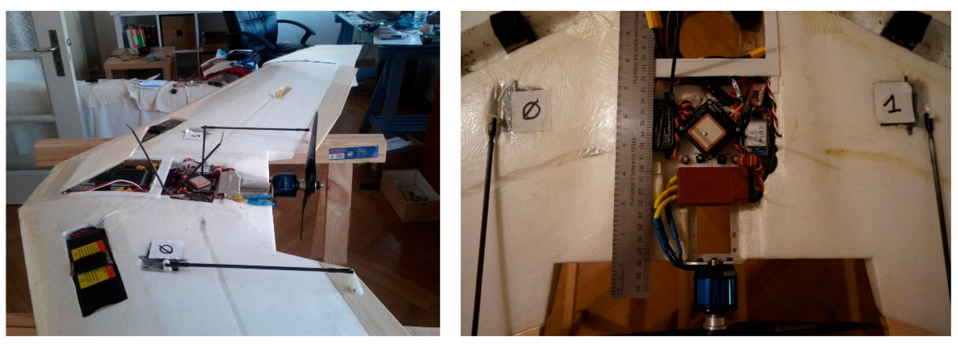
The UAV was an electric powered Styrofoam delta shaped fixed wing UAV equipped with a flight controller and a camera. Its width was 156 cm and it weighed about 2.1 kg with batteries and camera (Figure 1). The system had two elevons controlling pitch and roll, was powered by a set of lithium-polymer batteries and could achieve a flight time of ~1 h. The flight controller followed an approach standard to most flight micro-UAV flight controller systems [12]. A central processing unit interpreted attitude information from an inertial measurement unit and positional information from a Global Navigation Satellite System (GNSS).
The camera was a Sony NEX-5N with a 16.1 Megapixel APS-C CMOS sensor with rolling shutter coupled with a 16 mm lens. Images were acquired by the system in JPEG format every 50 m. The central processing unit recorded the position, attitude (roll, pitch, yaw), and speed of the UAV for each image. The GNSS, a Ublox model LEA-6H had a horizontal accuracy of ±2.5 m [13].
2.2. Description of the Study Area and Conditions during Data Collection
The study area was a portion of the Little Patuxent River (Albeth Heights, Howard County, Maryland (MD), USA) part of the Patapsco watershed (Patapsco River Lower North Branch Watershed). The Little Patuxent River has a basin area of 97 km2 and an average annual discharge of 1.41 m3s−1, with the dominant land cover being mostly forest and urbanized land. It is a rainfall-dominated, perennial runoff stream type characterized by high temporal variation in flow [14] and is thus prone to flash flooding during high rainfall events, such as during Hurricane Sandy and more recently the flash flood event in nearby Ellicott City and Columbia in July and August of 2016, which led to loss of lives, significant damage to infrastructure and evacuations, and resulted in Howard County being declared State of Emergency [15].
Over the small study site (Figure 2), we collected 429 JPEG images during leaf-off conditions (recommended for DEM acquisition, particularly for hydrological studies, to avoid tall vegetation in full canopy near river banks, easily obstructing all or large parts of the river, and/or on a floodplain) on March 11 2014 around midday, the weather was cloudy with no wind. We followed recommendations from [4] with a 60% lateral and 80% forward image rate of overlap. The flight pattern was a lawn and mower type with two complete overlapping patterns to increase photo overlap. Each image had an associated metadata file with the geographic location and attitude of the camera at the time of capture.
2.3. Using a Structure from Motion Algorithm to Create a Digital Surface Model
The SfM workflow is available as a standard algorithm in a number of open-source software packages, such as VisualSFM as described in [7], and typically comprises the following main processes: (i) detecting and matching distinct features from overlapping images; (ii) generating sparse point clouds; (iii) clustering the sparse point cloud and (iv) densifying the sparse point cloud. For these processes we used the algorithms packaged in Agisoft Photoscan Pro v1.0.
We chose to calibrate the lens parameters using a checker board and the lens software from Agisoft. We then fed the camera calibration parameters as initialization parameters for the bundle adjustment. We also excluded any image with a deviation from Nadir higher than six degrees to yield better accuracy. The GPS location error of each camera was set to 10 meters to account for Inertial Measurement Unit (IMU) drift and camera trigger lag.
The settings for the image alignment were: Point limit 40000, Accuracy High, pair preselection: ground control. Note that no ground control points were used. The pair preselection is based on the Camera GPS coordinates from the onboard GPS. We then ran optimize alignment to fit all parameters but the k4 coefficient. Finally, the point cloud generation was set to very high and aggressive filtering. Of course, the non-usage of GCPs increased the overall error (see for instance [17] for optimal GCP collection and usage) but it was difficult to estimate by how much since this depends on many processing factors, flying variables and also the complexity of the terrain. In this study, part of the objective was also to demonstrate adequacy of rapid mapping of local area detail, so without resource- and time-intensive collection of GCPs.
In order to properly compare both datasets, LIDAR point cloud and drone point cloud, they need to be in the same vertical and horizontal reference system. Due to the shift between the World Geodetic System of 1984 and the North American Datum of 1983 due to tectonic plates movements (CORS 96 NOAA) and GPS positional improvements (HARN NOAA) an incorrect datum could lead to an error measurement of up to one meter in the vertical plane [18]. In order to obtain the most accurate spatial positioning of the point cloud we used a 14-parameter transformation. We projected our UAV point cloud into the LiDAR projection (NAD83 NSRS 2007) using Vdatum, one of the only free software allowing a 14-parameter datum conversion with an accuracy of 7 cm [19] (we also accounted for WGS 84 to State plane drift by using the latest WGS84 ellipsoid EPOCH (ITRF2008 in Vdatum) and transit through the latest NAD83 EPOCH (NAD 83 HARN)).
2.4. Comparison between LiDAR and Drone DEM
2.4.1. LiDAR Data Description
The State of Maryland contracted the collection of detailed ground elevation data from aerial LiDAR in 2011 for approximately 663 km2 over Howard County (MD, USA) as part of the CATSII, 2011 Maryland State-wide Orthophoto Project. The LiDAR data were collected in accordance with FEMA procedures on data format and delivery and USGS LiDAR technical guidelines and specifications. The data were processed to bare-earth and vertical accuracy was assessed following the National Digital Elevation Program (NDEP)/American Society for Photogrammetry and Remote Sensing (ASPRS) guidelines for fundamental vertical accuracy (FVA) (18.5 cm RMSEz), supplemental vertical accuracy (SVA), and consolidated vertical accuracy (CVA) (<=36.3 cm 95th percentile) [20,21]. Table 1 compares the main DEM properties of both systems for this particular study area. Note that the area of the UAV site is a lot smaller than the hydrological basin area or indeed the total coverage area of LiDAR, so, for the comparison analysis, the area of the LiDAR was limited to that of the UAV.
2.4.2. Preparation of UAV Point Cloud to Compare with LiDAR
The removal of low overlap areas from the UAV point cloud significantly improved the accuracy. We removed areas with less than nine images overlap. If the images have been properly collected, low overlaps will be at the edges of the model.
We selected the bare-earth LiDAR data and applied an algorithm to remove the vegetation from the UAV point cloud. The algorithm used was the Photoscan built-in function ‘Classify Ground Points’, and we used the following settings, which we believe to be sensible given the high-resolution, high-precision nature of the data: any point within a 50-meter moving window with maximum ground slope of four degrees, and the maximum elevation variation of more than 10 cm from the lowest point was excluded.
2.4.3. DEM Analysis
Since there is a non-trivial 3-year time gap between the UAV flight and the LiDAR campaign (2014 and 2011, respectively), the accuracy assessment of the elevation in the UAV data set using the LiDAR bare-earth point cloud data as reference presents only relative differences rather than actual errors. In fact, the assessment cannot be used to determine the more accurate data set because no independent height data, such as GCPs, were collected at the time of the UAV flight and any significant difference between the LiDAR and UAV may come from an actual topography change that occurred during the 3-year time gap; although we do believe that to be too short of a time gap for any significant change in topography to have occurred.
Nonetheless, the actual analysis was thought reasonable given the available data and straightforward. We read and queried the LiDAR point data in LAS format using MatlabTM (see [22] for functions). Following the UAV point cloud processing, we produced the UAV-(drone) DEM over the study site for an area 873 m long by 575 m wide and with a regular pixel spacing of 0.0681 m.
The assessment was carried out using the closest LiDAR bare-earth cloud point to every UAV-DEM pixel after basic vegetation correction as outlined in the previous section. We used a radial search based on geographic coordinates to select the closest LiDAR point. As accuracy, or rather difference metrics, we used the mean difference or deviation (MD) and root mean square deviation (RMSD), which are typical measures to assess height accuracy. MD and RMSD are defined as follows:
where zLiDAR denotes the LiDAR bare-earth elevation (m) and zRPS the UAV bare-earth elevation (m).
2.4.4. Characterizing First-Order Floodplain and Channel Hydraulics
A high-accuracy floodplain DEM is essential for adequate flow modeling and consequently flood risk estimation [23]. Substantial errors in the vertical can lead to considerable over- or underestimation of flood hazard which can have many adverse consequences. Any flood model requires data on river gradients, bank and floodplain heights, and for 1-D in-channel flood models such as HEC-RAS and also for 1-D/2-D coupled flood models this river information is provided as river section data. For this purpose, we assessed heights along the stream centerline of the Patapsco river in flow direction and impose a linear fit to estimate the thalweg gradient and first order hydraulics (i.e., kinematic waveform). To assess the quality of the floodplain topography we ran a simple flood-fill algorithm over parts of the river’s floodplain. Both analyses were performed on the LiDAR and drone SfM DEMs, using the former as a reference.
For flood-fill modeling we followed the procedure adopted by Schumann et al. [24]. This method is based on calculating a floodplain elevation profile from the digital terrain model (DTM) data (often referred to as bare earth DEM), which describes floodplain water depth as a function of flooded area [25]. For simplification, depth was given as an increasing function of flooded area so that no local depression was assumed in the floodplain elevation profile. This simplification was based on the assumption that inundation always occurs from lower to higher places within a unit catchment. Significant differences in cumulative distribution functions (CDFs) of floodable land of both DTMs can then be statistically assessed. Prior to this the natural floodplain was delineated using correlation between local valley slope and the topographic wetness index (TWI) [26], where high values typically denote converging, almost flat terrain at locations where large upslope areas are drained, a, and where the local gravitational gradient, b, is low. TWI is defined as follows:
3. Results and Discussion
3.1. Accuracy Assessment
As stated earlier, areas of low overlap, edges of the acquisition area, are not as accurate, and hence removing the low confidence, high-error edge areas from the analysis eliminated height bias (−1.6 cm) and reached an acceptable RMSD value of 39 cm. Even though GCPs are not used (or required), their absence may lead to systematic error in the model [27], the effects of which are not assessed in this study. The residual distribution of the LiDAR vs drone DEMs (Figure 3) exhibited a slight negative skew in the distribution (Figure 4).
Note that although horizontal accuracy has not been estimated (due to a lack of ground control points), we argue that the river cross-sectional geometry would be shifted in the horizontal or vertical plane by a nontrivial amount if the horizontal error were significant, which is clearly not the case here, as illustrated in the next section.
It should also be noted that vegetation removal could be improved using a more sophisticated classifier as developed and described for instance by [28], which in turn would probably lead to better vertical accuracy of the bare-earth UAV-DEM. Furthermore, camera capture time may vary but we believe this to be a negligible contribution.
3.2. River and Floodplain Characteristics
While variations of in-channel water levels (determined by local flow conditions) drive the timing and amount of water overtopping the river banks and spilling onto adjacent low-lying land, it is variations in floodplain topography that control floodplain flow paths and inundated area during a flood event. Thus, microtopography and floodplain features, such as buildings, walls, trees, etc., become important, particularly when interested in localized flow conditions and associated floodplain inundation at the small scale [29].
Also, as clearly illustrated in the drone DSM shown in Figure 2, there are considerable differences between the actual variability in stream geometry or topology and the rather over-simplified line geometry in vector datasets from high-end national GIS databases, such as NHDPlus in the U.S. Such big differences in small-scale features can have non-trivial consequences when used in applications such as flood wave modeling. The many challenges associated with accurately representing small-scale streams and other features in national databases like NHDPlus are well known and acknowledged [16], and here UAV-derived topography data can be an invaluable resource for updating such fundamental databases, at least in known problem locations.
In the context of flood modeling, microtopographic features and variations in microtopography (i.e., topographic variation about a mean surface trend with amplitudes much smaller than the hillslope or basin scales [30]) are only included in flood inundation (i.e., 2-D hydraulic) models if high-resolution, high-precision data on floodplain heights are available. However, in most cases the effects of microtopography on water flows are parameterized in flood models of grid resolutions typically orders of magnitude larger than the microtopographic controls [31].
Within this context, Mason et al. [29] state that the typical vertical accuracy of floodplain heights from airborne LiDAR (10 to 20 cm RMSE) provides a realistic lower limit for DEM quality as beyond this the sensor signal becomes indistinguishable from ‘noise’ generated by background microtopographic features. In line with this reasoning, it is fair to assume that a vertical error of 2σ of the lower limit (~40 cm) sets an adequate upper limit target value.
Examining first order channel hydraulics (slope and channel cross-section geometry) is also important due to the significance of in-channel water level variations as outlined above. According to the Rosgen classification of streams and their floodplains [32], our river and floodplain surveyed fall under type ‘E’, characterized by low gradient, meandering rivers of low width to depth ratios and stable, vegetated banks with broad valley floodplains.
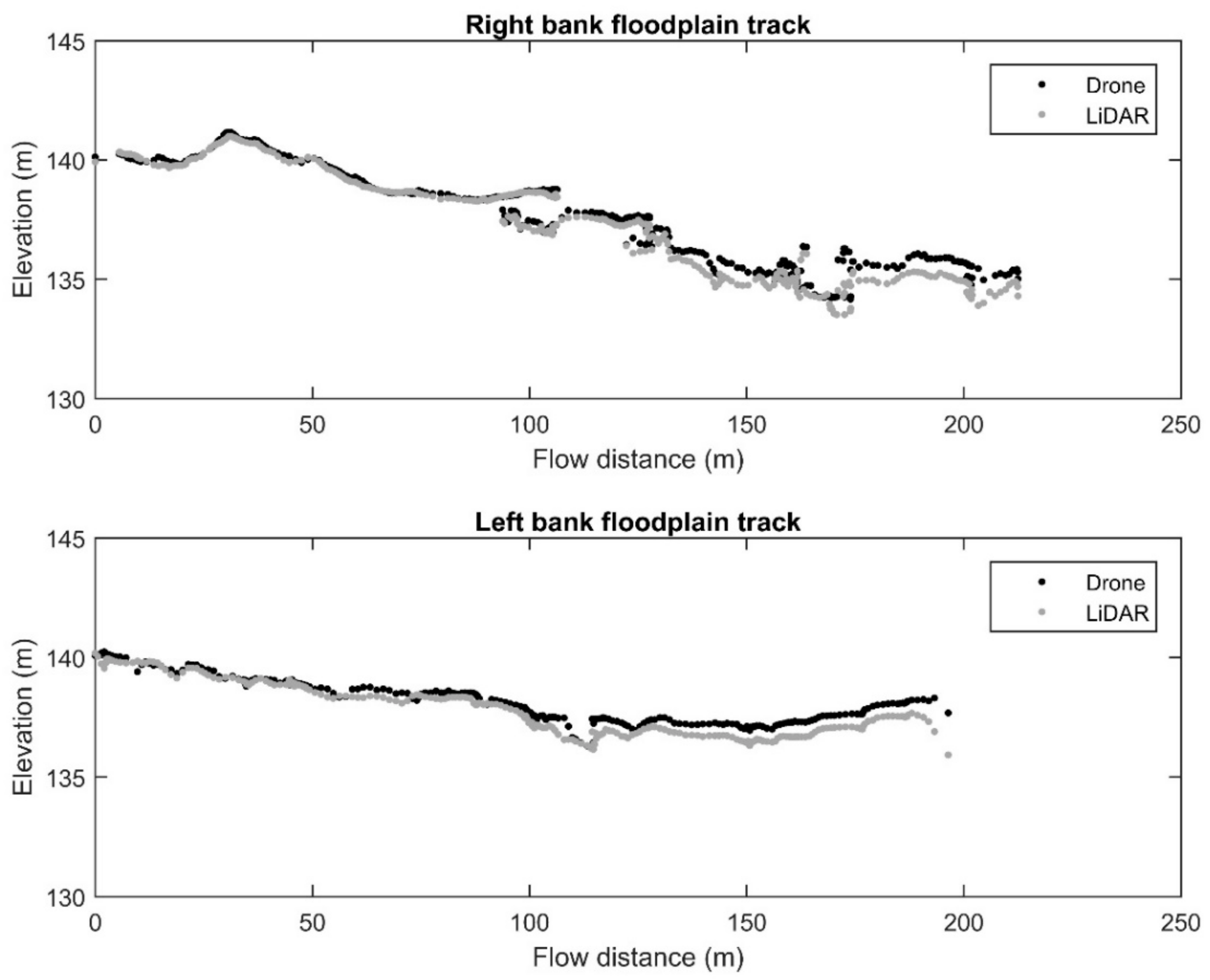
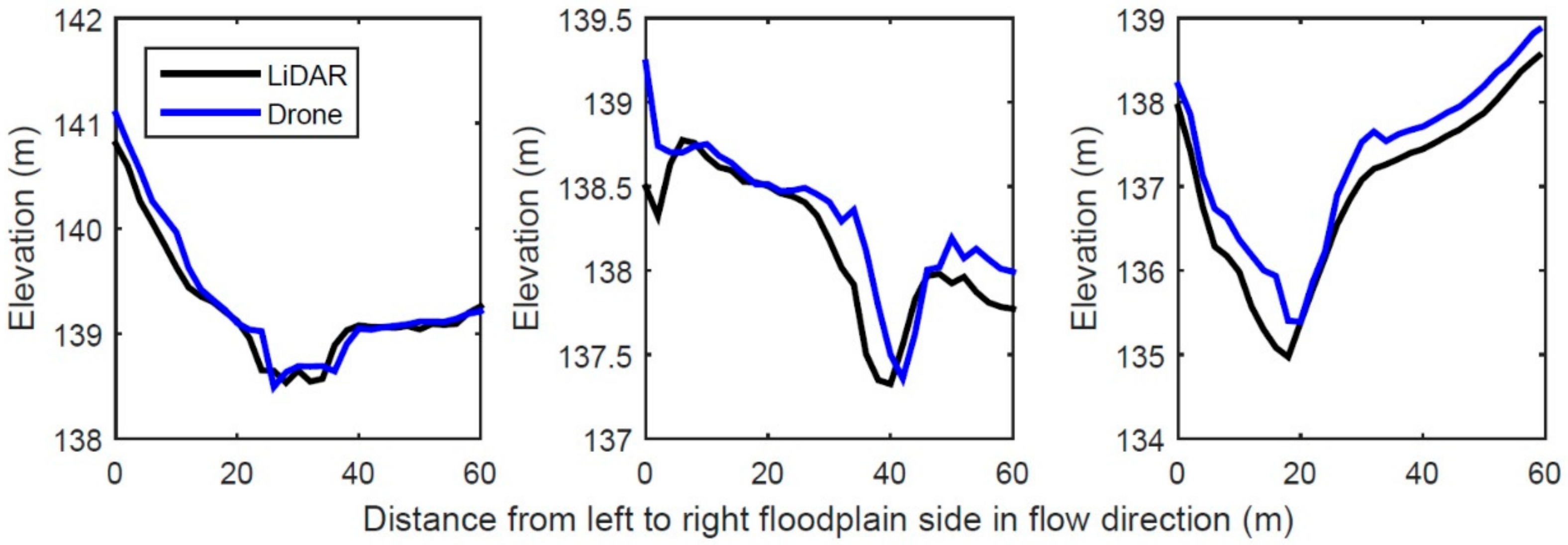
For this type of streams, Rosgen [32] defines a typical channel gradient of <0.02 and a width to depth (W/D) ratio of <12. If the DTM data are accurate (i.e., fall within the above stated height target range), we should expect similar river slope and W/D values for our site. For the stream surveyed, the river gradient falls between 0.017 and 0.031, for the left and right bank slope, with a bias of 0.34 m and 0.28 m, respectively (see Figure 5). For both banks, the RMSD is 0.44 m. The river cross-sections illustrated in Figure 6 also show the expected W/D ratio of <12.
These are acceptable accuracy values and are the same for the entire floodplain area depicted in Figure 7, with a bias of 0.28 m and a RMSD of 0.43 m. Note that this RMSD value is consistent with that obtained over the entire study area (Section A) but the floodplain exhibits a bias while there is negligible bias when considering the entire study area. We attribute this (positive) floodplain bias to the height of typical short floodplain vegetation (see e.g., [33]), which is probably difficult to remove with a basic vegetation removal algorithm that was applied here.
3.3. Implications for Flood Mapping and Prediction
In order to assess the applicability of the SfM DTM, we ran a simple flood-fill operation over the entire floodplain area (Figure 7), as explained in Section 2.4.4. The suitability of a DTM to map flooded area or to serve as the topographic boundary for accurate flood modeling and prediction can be determined on the basis of floodplain height profiling [25].
For this purpose, we plotted and compared the cumulative distribution function (CDF) of the elevation within the study region of the LiDAR DTM and the SfM DTM. As shown in Figure 7, there are only marginal differences in the elevation profiles from LiDAR and SfM. In fact, a two-sample Kolmogorov–Smirnov (KS) test indicates that, at a 5% α level, there are no significant differences between the two floodplain height distributions. The same is true when translating these heights to floodplain inundation as illustrated by the panels at the bottom of Figure 7.
4. Conclusions
These results indicate that the SfM DTM should yield nearly identical performances when used for flood mapping and prediction as those typically obtained from LiDAR. However, here, we only tested for basic characterization of in-channel hydraulics and floodplain inundation mapping and therefore recommend more complete investigations of the suitability of drone-acquired DTMs for flood modeling and mapping. In fact, in line with the conclusion drawn by Schumann et al. [24] for a novel airborne InSAR DEM technology, what is also needed here is a proper hydraulic modeling benchmark study, preferably using a floodplain and a flood event for which LiDAR data have been used.
Nevertheless, initial findings agree with traditional stream and floodplain classification theory and thus show very promising results for this type of UAV usage. We expect this type of UAV application to gain more momentum in the near future with the ever-growing importance of more detailed and better data to increase resilience to flood risk, especially in urbanized catchments. In line with the conclusions in Brazier et al. [10], there remain a wealth of opportunities for exploring UAV use in strengthening and improving scientific understanding of a broad spectrum of water resources applications for which aircraft or field campaigns prove too resource-intensive or too impractical.
Author Contributions
Conceptualization, G.J.-P.S., J.M., K.M.A.; Formal analysis, G.J.-P.S. and J.M.; Methodology, G.J.-P.S., J.M. and K.M.A.; Validation, G.J.-P.S.; Visualization, G.J.-P.S. and J.M.; Writing–original draft, G.J.-P.S. and J.M.; Writing–review & editing, G.J.-P.S., J.M. and K.M.A.
Funding
This research received no external funding.
Acknowledgments
We would like to thank Noah Snavely for helping us understand the complexities of Structure from Motion equations.
Conflicts of Interest
Joseph Muhlhausen was employed by WeRobotics. Guy J.-P. Schumann was employed by Remote Sensing Solutions. There is no financial interest for either company and the article does not necessarily reflect any company position or opinion. All authors declare no competing interests.
References
- Fonstad, M.A.; Dietrich, J.T.; Courville, B.C.; Jensen, J.L.; Carbonneau, P.E. Topographic structure from motion: A new development in photogrammetric measurement. Earth Surf. Process. Landf. 2013, 38, 421–430. [Google Scholar] [CrossRef]
- Snavely, N.; Seitz, S.M.; Szeliski, R. Modeling the world from Internet photo collections. Int. J. Comput. Vis. 2008, 80, 189–210. [Google Scholar] [CrossRef]
- Rosnell, T.; Honkavaara, E. Point cloud generation from aerial image data acquired by a quadrocopter type micro unmanned aerial vehicle and a digital still camera. Sensors 2012, 12, 453–480. [Google Scholar] [CrossRef]
- Bolognesi, M.; Furini, A.; Russo, V.; Pellegrinelli, A.; Russo, P. Accuracy of cultural heritage 3D models by RPAS and terrestrial photogrammetry. Int. Arch. Photogramm. Remote Sens. Spat. Inf. Sci. 2014, XL-5, 113–119. [Google Scholar] [CrossRef]
- Grenzdörffer, G.; Engel, A.; Teichert, B. The photogrammetric potential of low-cost UAVs in forestry and agriculture. Int. Arch. Photogramm. Remote Sens. Spat. Inf. Sci. 2008, 37, 1207–1214. [Google Scholar]
- Shahbazi, M.; Sohn, G.; Théau, J.; Ménard, P. UAV-based point cloud generation for open-pit mine modelling. Int. Arch. Photogramm. Remote Sens. Spat. Inf. Sci. 2015, XL-1/W4, 313–320. [Google Scholar] [CrossRef]
- Mlambo, R.; Woodhouse, I.H.; Gerard, F.; Anderson, K. Structure from motion (SfM) photogrammetry with drone data: A low cost method for monitoring greenhouse gas emissions from forests in developing countries. Forests 2017, 8, 68. [Google Scholar] [CrossRef]
- Kalacska, M.; Chmura, G.L.; Lucanus, O.; Bérubé, D.; Arroyo-Mora, J.P. Structure from motion will revolutionize analyses of tidal wetland landscapes. Remote Sens. Environ. 2017, 199, 14–24. [Google Scholar] [CrossRef]
- Bates, P.D. Remote sensing and flood inundation modelling. Hydrol. Process. 2004, 18, 2593–2597. [Google Scholar] [CrossRef]
- Brazier, R.E.; Jones, L.; DeBell, L.; King, N.; Anderson, K. Water resource management at catchment scales using lightweight UAVs: Current capabilities and future perspectives. J. Unmanned Veh. Syst. 2016, 4, 7–30. [Google Scholar]
- Mudd, S.M. Investigation of the hydrodynamics of flash floods in ephemeral channels: Scaling analysis and simulation using a shock-capturing flow model incorporating the effects of transmission losses. J. Hydrol. 2006, 324, 65–79. [Google Scholar] [CrossRef]
- Remes, B.; Hensen, D.; Van Tienen, F.; De Wagter, C.; Van Der Horst, E.; De Croon, G. Paparazzi: How to make a swarm of Parrot AR Drones fly autonomously based on GPS. In Proceedings of the International Micro Air Vehicle Conference and Flight Competition (IMAV), Toulouse, France, 17–20 September 2013. [Google Scholar]
- u-blox. GPS: Essentials of Satellite Navigation Compendium; GPS-X-02007-D; u-blox AG: Thalwil, Switzerland, 2009. [Google Scholar]
- Poff, N.L.R.; Tokar, S.; Johnson, P. Stream hydrological and ecological responses to climate change assessed with an artificial neural network. Limnol. Oceanogr. 1996, 41, 857–863. [Google Scholar] [CrossRef]
- Janney, E. Maryland Governor Declares Howard County in State of Emergency. Available online: https://patch.com/maryland/ellicottcity (accessed on 1 August 2016).
- Moore, R.B.; Dewald, T.G. The Road to NHDPlus—Advancements in Digital Stream Networks and Associated Catchments. J. Am. Water Resour. Assoc. 2016, 52, 890–900. [Google Scholar] [CrossRef]
- Gindraux, S.; Boesch, R.; Farinotti, D. Accuracy assessment of digital surface models from Unmanned Aerial Vehicles’ imagery on glaciers. Remote Sens. 2017, 9, 186. [Google Scholar] [CrossRef]
- Craymer, M.R. The evolution of NAD83 in Canada. Geomatica 2006, 60, 151–164. [Google Scholar]
- NOAA Vdatum: Vertical Datum Transformation. Available online: https://vdatum.noaa.gov/ (accessed on 8 December 2016).
- Flood, M. ASPRS Guidelines: Vertical Accuracy Reporting for LiDAR Data; ASPRS: Bethesda, MD, USA, 2004. [Google Scholar]
- MDiMap Maryland’s Mapping and GIS Portal: LiDAR Metadata. Available online: https://imap.maryland.gov/Pages/lidar-metadata.aspx (accessed on 27 February 2019).
- Pingel, T.J. Lasread-Matlab: LiDAR Binary Reader for Matlab. Available online: https://github.com/thomaspingel?tab=repositories (accessed on 11 July 2016).
- Bates, P.D. Integrating remote sensing data with flood inundation models: How far have we got? Hydrol. Process. 2012, 26, 2515–2521. [Google Scholar] [CrossRef]
- Schumann, G.J.-P.; Moller, D.K.; Mentgen, F. High-Accuracy Elevation Data at Large Scales from Airborne Single-Pass SAR Interferometry. Front. Earth Sci. 2016, 3, 88. [Google Scholar] [CrossRef]
- Yamazaki, D.; Kanae, S.; Kim, H.; Oki, T. A physically based description of floodplain inundation dynamics in a global river routing model. Water Resour. Res. 2011, 47, W04501. [Google Scholar] [CrossRef]
- Beven, K.J.; Kirkby, M.J. A physically based, variable contributing area model of basin hydrology. Hydrolol. Sci. Bull. 1979, 24, 43–69. [Google Scholar] [CrossRef]
- Bakker, M.; Lane, S.N. Archival photogrammetric analysis of river–floodplain systems using Structure from Motion (SfM) methods. Earth Surf. Process. Landf. 2017, 42, 1274–1286. [Google Scholar] [CrossRef]
- Brodu, N.; Lague, D. 3D terrestrial lidar data classification of complex natural scenes using a multi-scale dimensionality criterion: Applications in geomorphology. ISPRS J. Photogramm. Remote Sens. 2012, 68, 121–134. [Google Scholar] [CrossRef]
- Mason, D.C.; Cobby, D.M.; Horritt, M.S.; Bates, P.D. Floodplain friction parameterization in two-dimensional river flood models using vegetation heights derived from airborne scanning laser altimetry. Hydrol. Process. 2003, 17, 1711–1732. [Google Scholar] [CrossRef]
- Thompson, S.E.; Katul, G.G.; Porporato, A. Role of microtopography in rainfall-runoff partitioning: An analysis using idealized geometry. Water Resour. Res. 2010, 46, W07520. [Google Scholar] [CrossRef]
- Dottori, F.; Di Baldassarre, G.; Todini, E. Detailed data is welcome, but with a pinch of salt: Accuracy, precision, and uncertainty in flood inundation modeling. Water Resour. Res. 2013, 49, 6079–6085. [Google Scholar] [CrossRef]
- Rosgen, D.L. A classification of natural rivers. Catena 1994, 22, 169–199. [Google Scholar] [CrossRef]
- Cobby, D.M.; Mason, D.C.; Davenport, I.J. Image processing of airborne scanning laser altimetry data for improved river flood modelling. ISPRS J. Photogramm. Remote Sens. 2001, 56, 121–138. [Google Scholar] [CrossRef]
Figure 1.
Photos of the electric powered Styrofoam delta shaped fixed wing Unmanned Aerial Vehicle (UAV) used in this study.
Figure 1.
Photos of the electric powered Styrofoam delta shaped fixed wing Unmanned Aerial Vehicle (UAV) used in this study.

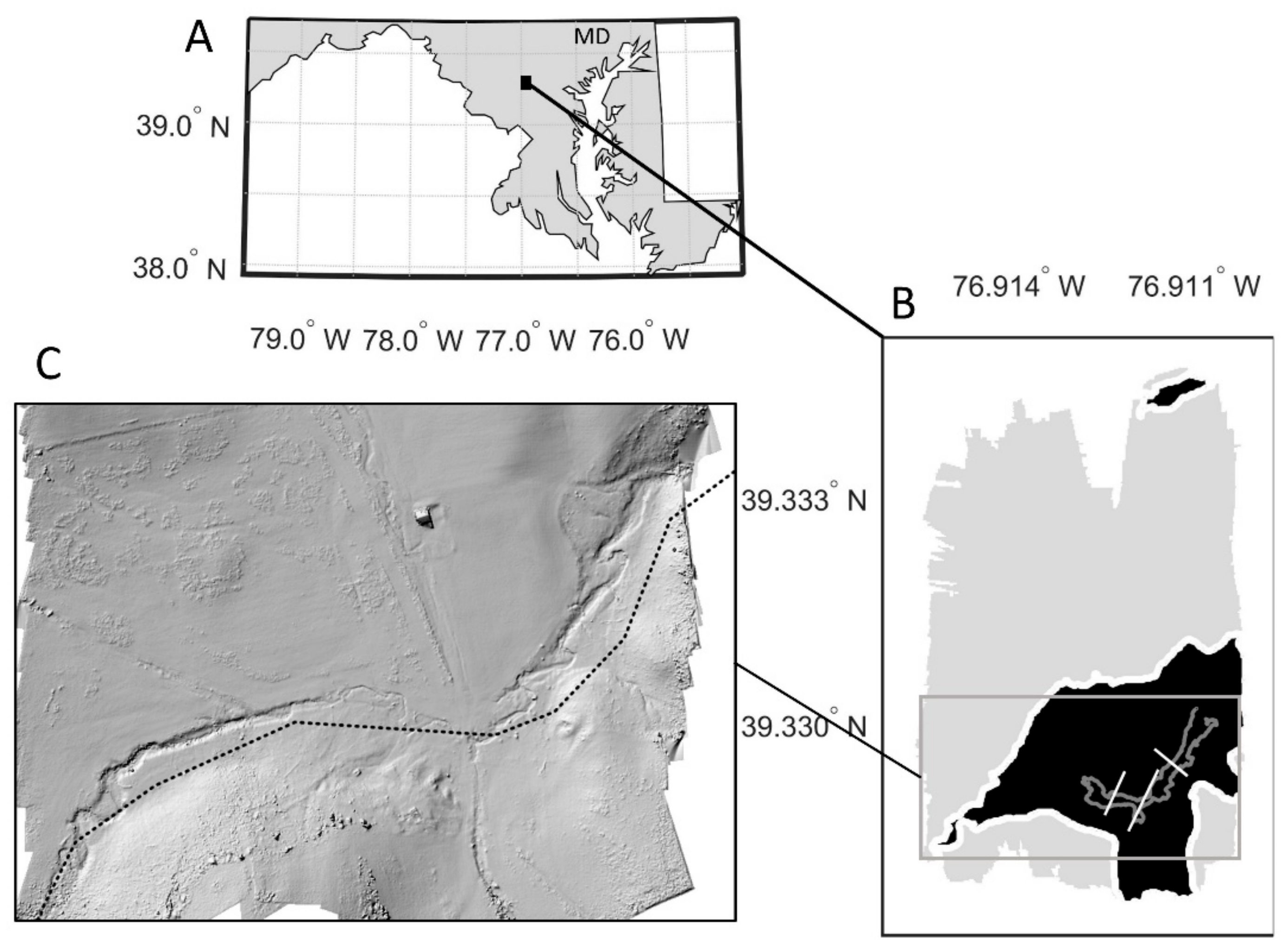
Figure 2.
(A) Map of study site located near Marriottsville (Howard County, MD). A zoom-in of the floodplain area is also shown in the bottom right (B). Traces of the river banks and river cross-sections perpendicular to flow direction are overlain (refer to main body of text for more details). The image in the bottom left (C) is the digital surface model (DSM) from the drone and shows the USGS NHDPlus [16] stream centerline (flowline) as a dashed black line. Note the deviation of the rather straight-line geometry of the NHDPlus flowline from the actual, highly complex, stream topology as depicted in the drone DSM.

Figure 3.
LiDAR (A) and drone (B) bare earth elevation models for the area depicted in Figure 2. Elevation contour lines are overlain. Note that topography is only marginally different between the two datasets.
Figure 3.
LiDAR (A) and drone (B) bare earth elevation models for the area depicted in Figure 2. Elevation contour lines are overlain. Note that topography is only marginally different between the two datasets.

Figure 4.
Distribution of the residual difference between the LiDAR and the drone elevation data. There is a slight negative skew of the distribution which could indicate a small systematic error in the drone elevation data.
Figure 4.
Distribution of the residual difference between the LiDAR and the drone elevation data. There is a slight negative skew of the distribution which could indicate a small systematic error in the drone elevation data.

Figure 5.
Heights along GPS traces of right (top panel) and left (bottom panel) river bank are shown. For accuracy assessment, see main body of text.
Figure 5.
Heights along GPS traces of right (top panel) and left (bottom panel) river bank are shown. For accuracy assessment, see main body of text.

Figure 6.
Sample river cross-sections (drawn perpendicular to flow direction). Cross-sectional elevations reveal in-channel depth topology. For locations of cross-sections, see Figure 2. We attribute the non-trivial horizontal shift of the section in the middle graph to changes in cross-section geomorphology in-between acquisition dates of the LiDAR and drone datasets; however, there is no clear evidence for this. Note that in both cases, the river was in very low flow conditions, so we expect a fairly accurate channel depth estimation from both datasets.

Figure 7.
Floodplain fill operations for LiDAR (C) and drone (D) DTMs as well as the cumulative distribution function (CDF) of floodplain heights (B). Contour lines at 2 m height intervals are shown in blue on the images. Note that the “probability of inundation” from the CDF (y-axis) in B indicates the “probability” of the entire floodplain area (shown in black in (A)) being inundated at a given floodplain height (x-axis).


Table 1.
Table comparing LiDAR and UAV digital elevation model (DEM) characteristics.
| Property | LiDAR | UAV Scene |
|---|---|---|
| Spheroid | Global Reference System 1980 | World Geodetic System 1984 |
| Horizontal Datum | North American Datum 83 | World Geodetic System 84 (1674) |
| Vertical Datum | North American Datum 83 (NSRS 2007) | International Terrestrial Reference Frame 2008 |
| Coordinate system | State Plane 1900 | Universal Transverse Mercator 18N |
| Point spacing | 1.4 m | 0.068 m |
| Scene/Relative accuracy | 18.5 cm RMSEz | 0.98 pixel = 3.32 cm (Agisoft scene error) |
© 2019 by the authors. Licensee MDPI, Basel, Switzerland. This article is an open access article distributed under the terms and conditions of the Creative Commons Attribution (CC BY) license (http://creativecommons.org/licenses/by/4.0/).
Share and Cite
MDPI and ACS Style
Schumann, G.J.-P.; Muhlhausen, J.; Andreadis, K.M. Rapid Mapping of Small-Scale River-Floodplain Environments Using UAV SfM Supports Classical Theory. Remote Sens. 2019, 11, 982. https://0-doi-org.brum.beds.ac.uk/10.3390/rs11080982
AMA Style
Schumann GJ-P, Muhlhausen J, Andreadis KM. Rapid Mapping of Small-Scale River-Floodplain Environments Using UAV SfM Supports Classical Theory. Remote Sensing. 2019; 11(8):982. https://0-doi-org.brum.beds.ac.uk/10.3390/rs11080982
Chicago/Turabian StyleSchumann, Guy J.-P., Joseph Muhlhausen, and Konstantinos M. Andreadis. 2019. "Rapid Mapping of Small-Scale River-Floodplain Environments Using UAV SfM Supports Classical Theory" Remote Sensing 11, no. 8: 982. https://0-doi-org.brum.beds.ac.uk/10.3390/rs11080982
Note that from the first issue of 2016, this journal uses article numbers instead of page numbers. See further details here.