Integration of Corner Reflectors for the Monitoring of Mountain Glacier Areas with Sentinel-1 Time Series

Abstract

Glacier flow and slope instabilities in Alpine mountain areas represent a hazard issue. Sentinel-1 satellites provide regular Synthetic Aperture Radar (SAR) acquisitions that are potentially useful to monitor these areas, but they can be affected by temporal decorrelation due to rapid changes in the surface. The application of interferometric synthetic aperture radar (InSAR) therefore seems difficult due to loss of coherence. On the other hand, Corner Reflectors (CR) can be used as coherent targets in SAR images for accurate displacement measurement thanks to their strong backscattering property and temporal stability. The use of CRs in multi-temporal InSAR analysis in Alpine mountain areas can thus be beneficial. In this study, we present a comparison between triangular and rectangular CRs, based on Radar Cross Section (RCS) measurements in an anechoic chamber and on long-term experiments over the Argentière glacier and the surrounding slopes and moraine. The visibility in both summer and winter of 10 CRs installed on the test site was investigated. As this area is exposed to heavy precipitation including snow falls, two perforated CRs were tested. The amplitude stability and the phase error of each CR were estimated. A precise tracking of two CRs installed at the glacier surface was also able to measure the displacement of the Argentière glacier, giving results close to previous GPS measurements. Furthermore, a Persistent Scatterer Interferometry (PSI) study was conducted, using the most stable CR as reference point to estimate slope instabilities, which led to the identification of an area corresponding to a tectonic fault called “Faille de l’angle”. The precise absolute locations of the CRs were successfully estimated and PS heights were compared with a LiDAR-based (Light Detection And Ranging) digital elevation model (DEM) and GPS measurements.

1. Introduction

The application of Interferometric Synthetic Aperture Radar (InSAR) for ground displacement monitoring in mountainous areas may present certain limitations due to coherence loss [1]. Snow falls, the melting of ice and snow and high shear gradients over glaciers introduce rapid changes in the scene reflectivity. Outside the glaciers, many moving zones related to the creep of frozen debris (rock glaciers, pushmoraines), shallow to deep-seated landslides affecting frozen and unfrozen debris or rocks [2], can also be sources of temporal decorrelation. In such cases, an appropriate use of artificial corner reflectors (CR) can be helpful to overcome these limitations.

CRs behave like point targets, providing a strong backscattering response in SAR images [3,4]. They are characterized by a much higher reflectivity than the surrounding scatterers, by a high Radar Cross-Section (RCS) and a high signal-to-noise ratio (SNR) [5,6]. The response of large size CRs considerably dominates the echo of the resolution cell so that the peak of the impulse response function contains practically no contribution from the ground [5]. Since CRs provide stable interferometric phase and accurate displacement estimation, they have been used in many applications: targets in SAR image calibration [7,8], artificial Persistent Scatterers (PS) to increase the density of PSs for landslide monitoring [9,10] and ground subsidence monitoring [11] or for detecting surface deformations due to $C{O}_2$ injection [12] as well as for glacier monitoring [13]. CRs can overcome the temporal decorrelation problem and also to eliminate the residual phase error of the topographic component and also minimize error due to atmospheric delays by combining CR-InSAR with GPS [14]. In C-band data, displacement errors smaller than a millimeter are achievable for CRs of 1.5 m or larger [4]. However, the larger the CR, the bigger the wind surface area, which requires a more secure and expensive hold, especially in mountainous areas where the wind can be very strong. One of the objectives of this study is to find a compromise between the size to make the contribution of the ground negligible and a low cost installation. Another goal is to test the performance of perforated CRs that have been designed to reduce the impact of mountainous meteorological conditions on the stability. Perforation should reduce the effect of wind and allow quick drainage of heavy rain and cleaning of dust [15]. The effects of perforations on CRs have been presented for X-band [16,17], but fewer research projects have been completed for C-band. However, a weaker influence of perforation is expected on C-band response than on X-band response [4,18]. A comparison is also presented between different triangular and rectangular trihedral shaped CRs. The RCS peaks of three different CRs were measured in an anechoic chamber to test the orientation sensitivity. Finally, 10 CRs were used for a number of experiments: five in a grass field in Choisy (France) and four of these and five other CRs on the Argentière glacier and on the surrounding slopes in the Chamonix–Mont-Blanc valley (France), to evaluate their visibility in the Sentinel-1 image time series. The geolocation accuracy of the CRs and instability of the slopes surrounding the Argentière glacier were investigated by a Permanent Scatterer Interferometry (PSI) approach.

This paper is organized as follows: Section 2 presents theoretical calculations and experimental results of RCSs in an anechoic chamber. Section 3 presents CRs’ detection using spectral correlation with an estimation of their visibility and the expected phase error based on the Signal-to-Clutter Ratio (SCR). Section 4 discusses the results of the estimation of Argentière glacier motion and presents the results of slopes monitoring by an ad hoc processing inspired by PSI. Results of the CRs’ absolute location are also discussed. The final section presents the conclusions.

2. Radar Cross-Section

RCS is the measure of a target’s ability to reflect radar signals in the direction of the radar receiver. The RCS of a CR should be large compared to its size [19,20]. Several shapes of CRs have been designed in the literature [3,16,17], with an RCS that is more or less sensitive to the orientation (i.e., azimuth and elevation angles). In this section, theoretical RCSs based on geometrical optics are presented for the 10 CRs used in this study (Figure 1). RCS measurements of three CRs (CR1, CR2 and CR3) achieved in an anechoic chamber are then presented.

2.1. Theoretical Estimation from Geometrical Optics

If we consider the radar wave as a plane wave illuminating a CR, its theoretical RCS can be calculated using equations derived from geometrical optics. The RCS then depends on the length of the sides of the CR, the radar wavelength and the orientation of the CR. This section presents a comparison of RCS between three different trihedral CRs: triangular, conventional perforated triangular (i.e., plates with holes) and perforated rectangular.

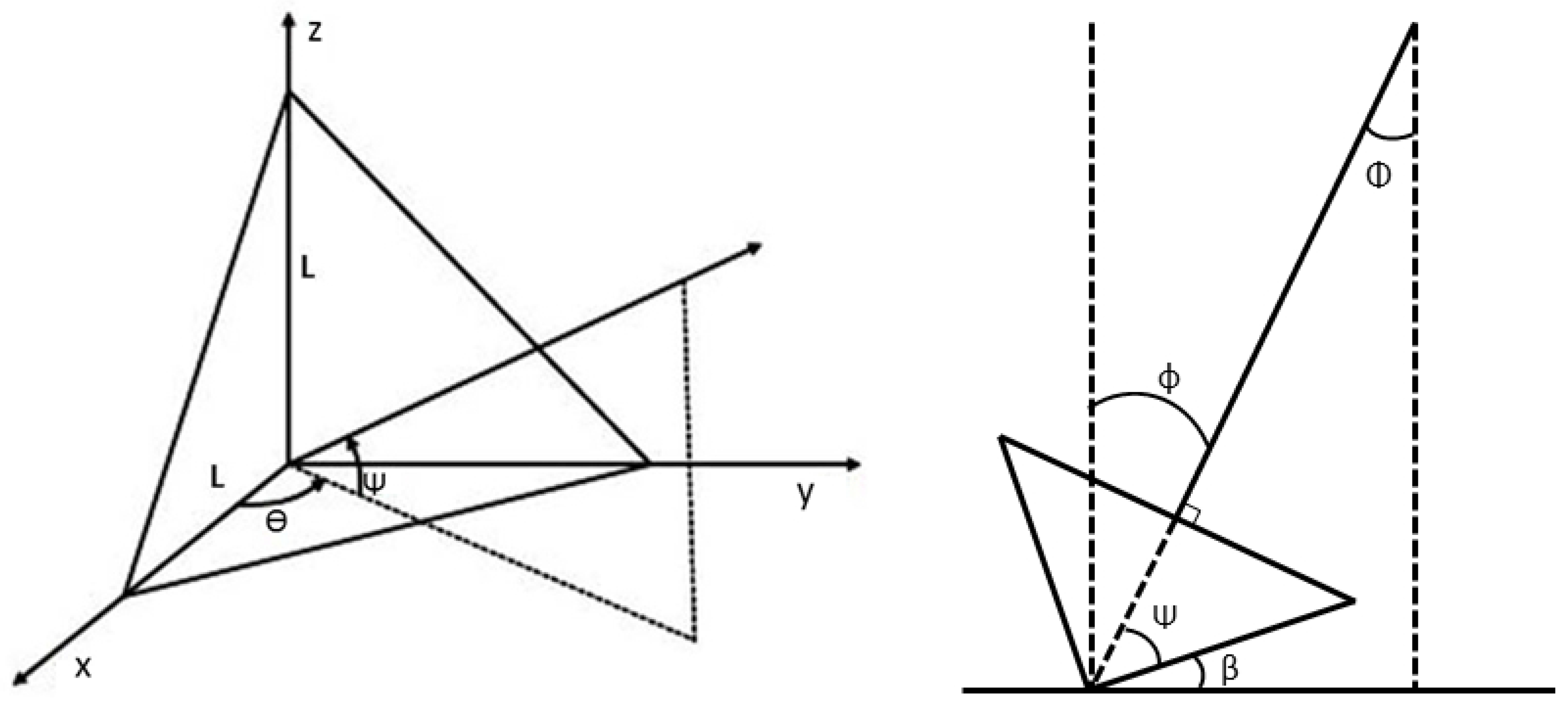
2.1.1. Triangular Trihedral Corner Reflectors

The conventional CR used for calibration or as PS is trihedral and made of isosceles right triangular plates [16]. The RCS peak of such a trihedral is calculated using geometrical optics as follows:

$${\sigma }_{triangle}=\frac{4\pi L^4}{3{\lambda }^2},$$

(1)

where L is the length of the sides of the CR (Figure 2) and $\lambda$ is the wavelength. This assumes that the edge dimension L is large relative to the wavelength. However, the observable RCS in radar image depends on the configuration of the CR, i.e., the RCS varies according to its azimuth orientation and elevation angles. We can consider a trihedral CR as an object whose RCS depends on its open face. The direction of the maximum RCS is defined as normal to the open face of the CR. Thus, in the case of an orientation angle $\theta =45$° (see Figure 2), the radar wave is normal to the open face when the elevation angle $\mathsf{\Psi }$ is equal to ${tan}^{-1}(\frac{1}{\sqrt[]{2}})$, so around 35.26° with one of the side plates [21,22].

In this study, we have tested triangular trihedral CRs with three different sizes. Their theoretical RCS peaks are summarized in

Table 1. Theoretical Radar Cross-Section $RC{S}_{th}$ and measured $RC{S}_m$ (dBm${}^2$) in an anechoic chamber for different side lengths and shapes of CRs in C-band (${}^c$) with $\lambda$ = 5.6 cm and X-band (${}^x$) with $\lambda$ = 3.1 cm. T = Triangular, R = Rectangular, Perf. = Perforated.

-	Shape	Side Length	${\mathit{RCS}}_{\mathit{th}}^{\mathit{C}}$	${\mathit{RCS}}_{\mathit{m}}^{\mathit{C}}$	${\mathit{RCS}}_{\mathit{th}}^{\mathit{X}}$	${\mathit{RCS}}_{\mathit{m}}^{\mathit{X}}$
		(mm)	(dBm${}^2$)	(dBm${}^2$)	(dBm${}^2$)	(dBm${}^2$)
CR1, CR4, CR5	T	955	30.46	26.76	35.59	30.77
CR2	Perf. T	955	30	26.44	35	30.60
CR3	Perf. R	500	26.46	24.02	33.89	26.46
CR 6, CR8, CR9	T	700	25.06	-	30.20	-
CR7, CR10	T	450	17.38	-	22.52	-

.

2.1.2. Rectangular Trihedral Corner Reflectors

Triangular trihedral corner reflectors are interesting because of their low sensitivity to azimuth and elevation settings [5]. However, for the same size of CR, there are other shapes which can provide a larger RCS. Square trihedral CRs offer a larger RCS than triangular trihedral CRs, very close to that of a circular one (quarter disk), and the production of a square trihedral is easier than that of a circular one [17]. Rectangular and square CRs have almost the same backscattering properties, but the former can have a larger RCS depending on the elevation angle. It can be interesting to set up a CR with a large elevation angle. In this way, ground interactions can be reduced [23], but the setting doesn’t allow to reach the RCS peak. This can be compensated by using rectangular upper plates. By lengthening the upper plates, the rectangular CR can reduce the loss of RCS due to incidence angles smaller than the one for which the CR is set up (i.e., with an elevation angle of 35°). In this way, this geometry can be used for different SAR sensors with different incidence angles, e.g., Sentinel-1 (from 29.1° to 46°) and TerraSAR-X (from 20° to 45°).

The theoretical RCS for a square trihedral CR is given by:

$${\sigma }_{square}=\frac{12\pi L^4}{{\lambda }^2},$$

(2)

where L is the length of the basal square sides of the CR and $\lambda$ is the wavelength. Thus, a RCS of 30 dB in C-band can be reached with a triangular CR of 930-mm side, while it can be reached with a square CR of only 540-mm side.

In this study, we worked with a rectangular CR comparable with those used in [11,17]. The rectangular corner is made of a basal square plate and two rectangular side plates. In this way, geometrical optics are not able to calculate the RCS. An RCS estimation approach for rectangle-type trihedral corners was proposed in [24]. This method used geometrical and physical optics to describe the backscattering RCS formula by the integration of multiple reflection contributions. The surface integration due to single reflection is evaluated over the whole area of the plate since it is completely illuminated. However, for double and triple reflections, the surface integration is only the illuminated parts of the second and third plates, whose shape is difficult to determine [20]. In our study, we only used the RCS formula obtained from geometrical optics. Throughout this paper, the theoretical RCS peak of a rectangular trihedral CR will be approximately estimated by the formula used for square trihedral CR, by taking the basal square plate side as reference length. In this way, the RCS value is underestimated. The true RCS was estimated in an anechoic chamber in Section 2.2.

2.1.3. Perforated Corner Reflectors

CRs are designed to be installed outdoors over long periods, and possibly for several years. As a result, the installations are exposed to meteorological conditions such as wind and precipitation (i.e., rain and snow falls). These conditions can cause instabilities in the CRs. One way to limit this source of error is to use plates with holes. In this way, wind forces are limited and precipitation can escape. Moreover, the weight of the CR is reduced, which is more practical.

In this study, we developed a perforated triangular CR (CR2) with L = 955 mm and a perforated rectangular CR (CR3) (Figure 1), composed of one basal square plate of 500-mm side and two rectangular plates (500 mm and 750 mm, respectively). The effects of these plates are investigated for both shapes.

In X-band, we saw that using perforated plates with holes of one-sixth of the wavelength reduces the maximum RCS by about 1 dB [15]. In this study, we used a CR with 1-cm holes, with Sentinel-1 data characterized by a wavelength of 5.6 cm. The RCS of perforated models and models without holes are expected to be close.

2.2. Measurements in an Anechoic Chamber

The objective of RCS measurements in an anechoic chamber is twofold: (1) to know the maximum RCS that can be obtained in an ideal case; (2) to measure the sensitivity of the RCS to the azimuth/elevation settings. These measurements can then provide recommendations on the settings for later installations of CRs obtained from RCS measurements in an anechoic chamber.

2.2.1. Principles of RCS Estimation

An anechoic chamber is an armored room whose walls and ceiling have been covered by electromagnetic absorbers that scatter or absorb the incident energy to simulate free space conditions [25]. These absorbers are produced from a material with absorbent qualities, known as loss material. The chamber used for the measurements in this study was covered with pyramidal absorbers (geometric transition absorbers). They consist of a matrix of polyurethane foam almost transparent to electromagnetic waves which is loaded with carbon (the most commonly used material with high dielectric losses). The pyramidal absorbers are covered with a polymerized acrylic binder to fix the carbon particles in the cells of the foam [26].

The approach here is based initially on the use of a reference target (an 18-inch disk) with a known RCS. It is therefore possible to obtain the relative RCS of other objects by comparison. The measured RCS, $RC{S}_m$, of a CR can be obtained by measuring the antenna gain from the following equation:

$$RC{S}_m=RC{S}_{ref}\times {10}^{\frac{G_m-G_{ref}}{10}}$$

(3)

where $RC{S}_{ref}$ is the RCS of the reference disk, $G_m$ is the measured gain and $G_{ref}$ the gain obtained from the reference disk.

The RCS measurements were done in C-band (5.405 GHz) and X-band (9.65 GHz), which gives a comparison of antenna gain between C-band and X-band.

Three different trihedral CRs were tested: a conventional triangular CR with L = 955 mm (CR1), a perforated triangular CR with L = 955 mm (CR2) to measure the effect of the holed plates, and a perforated rectangular CR with upper rectangular plates of 500 mm × 750 mm and a basal square plate of 500 mm (CR3) to measure the effect of rectangular plates. The RCS peaks measured in C-band are reported in Table 1. The CRs were positioned and inclined so that the signal is normal to the open face of the CR. Radar sensors (transmitter and receiver) are horizontal, thus the plane passing through the three edges is vertical for triangular CRs. This position corresponds to the position with elevation angle $\mathsf{\Psi }$ equal to 35° and azimuth angle equal to 45°, which gives the measurement of the RCS peak.

2.2.2. Results of RCS Peak Estimation

The theoretical RCS of CR1 is 30.46 dBm${}^2$ in C band, whereas RCS obtained in an anechoic chamber is 26.76 dBm${}^2$ (Table 1). The loss of 3.7 dBm${}^2$ can have several origins. The thinness of the plates (2 mm) combined with the transport to the anechoic chamber location may have induced plate curvature. Furthermore, small curvatures were noticed for the basal plate, especially for the triangular perforated model. The presence of brackets used to join each plate and those sticking out from each side can be another source of RCS loss. These results highlight the difficulty in finding the best compromise between a low-cost construction and an effective design. The comparison of RCS between CR1 and CR2 shows a loss of only 0.3 dBm${}^2$ with holed plates. As expected, perforation does not induce a significant loss. Then, CR3 also shows a loss of around 2.4 dBm${}^2$ between the (underestimated) theoretical and the measured RCS in C band. However, no straightforward curvatures were noticed on this model.

2.2.3. Discussions

As expected, the measured RCS are smaller than the theoretical ones. Several factors which can introduce a loss of RCS compared to the theoretical value are listed in [4]. A RCS loss exceeding 10 dB can result from a 5 mm plate curvature in a 1.0 m trihedral CR in X-band [27]. As the RCS loss due to plate curvature is inversely proportional to the radar wavelength and the target size [4], such RCS loss should be lower in C-band. Another known factor is the orthogonality between the three plates. A deviation from the right-angle leads to a loss of RCS, with a more severe loss for the acute angle than the obtuse angle [28]. Effects of angle variations are more important as the size of the CR increases and the radar wavelength decreases [28].

Note that the RCS measurements are valid if the so-called Fraunhofer far-field condition ($R\ge \frac{2d^2}{\lambda }$) is verified, where R is the distance between the target and the radar antenna, d the larger dimension of the target [29]. For the 18-inch disk used as the reference target, it represents a minimal distance of 13.5 m in C-band. Measurements were carried out in an anechoic chamber of 20 m long, so the Fraunhofer far-field condition is fulfilled. For the triangular CR with a length side of 955 mm, the larger dimension is the hypotenuse of the triangular plates which is equal to 135 cm, so the minimal distance is 65 m in C-band. Therefore, the difference between the theory and the measurement can be partially explained by construction defaults as explained above, and partially by the fact that measurements were conducted in condition with R less than one-third of the far field criterion.

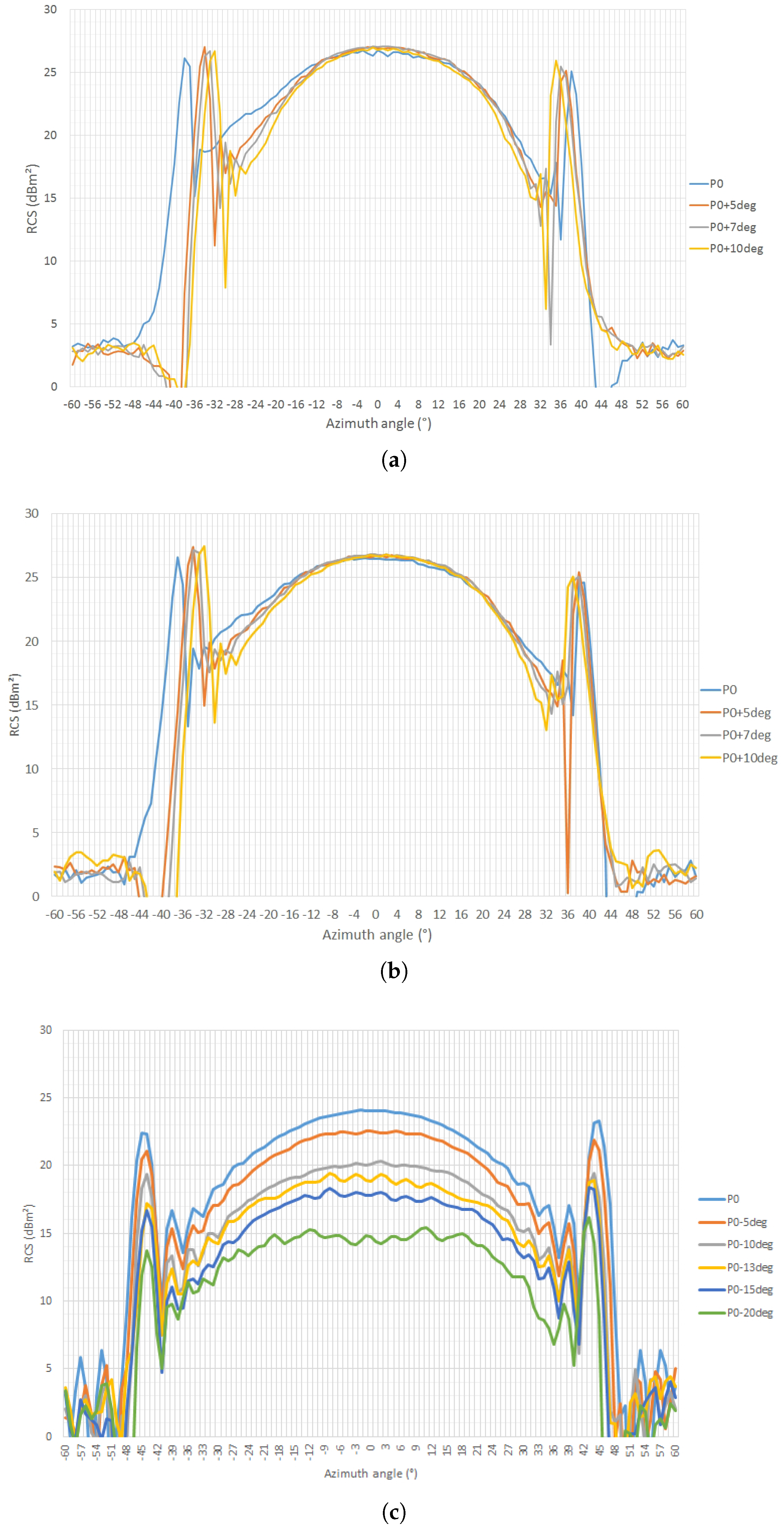
2.2.4. Setting Angle Sensitivity

Setting angle sensitivity was estimated by varying azimuth angle from the optimal position (Section 2.1.1) to $\pm 60$°, with a measurement at each degree. Operations were repeated with four different elevation angles kn C-band. The first set of measures of CR1, corresponding to the position $P0$, (blue curve in Figure 3a) shows a broad central part, which can be attributed to a triple-bounce mechanism between the three participating faces [30], with side lobes at each side of the central part, due to the single-bounce, and flat-plate scattering from the individual faces. A change of +/$-21$° from the optimal azimuthal position causes a symmetric decrease of only 3 dBm${}^2$. Thus, we can confirm that this triangular CR has a useful range of +/$-21$° for azimuth settings.

The following series (+5, +7 and +10 degrees from the optimal elevation angle) do not too much difference from the first one and present similar RCS peaks. The main observation is that, when the deviation of the elevation angle increases, the tolerance in azimuth setting decreases. Measurements with CR2 (Figure 3b) present very similar results. The useful ranges are close to those of CR1. Therefore, the presence of holes doesn’t seem to affect the setting sensitivity of the CRs. Figure 3c presents RCS measurements obtained with CR3, the rectangular perforated CR. In optimal elevation settings, CR3 presents a useful range (RCS loss less than 3 dBm${}^2$) of +/−21°. In the optimal azimuth setting, a deviation of 10° of the elevation angle induces a loss of 4 dBm${}^2$ of the RCS. With a deviation of 20°, the loss is around 10 dBm${}^2$. The rectangular model thus shows a slightly narrower useful cone and significant sensitivity to elevation settings.

2.2.5. RCS Performance Comparison between C-Band and X-Band

RCSs of CR1, CR2 and CR3 were also measured in X-band. The results presented in Figure 4 confirm that perforations with 1-cm-holes do not impact RCS, for either C-band or X-band. In X-band, the useful cone (decrease of 3 dBm${}^2$) is around 36°(−18/+18) in azimuth for CR1 and CR2. For CR3, the useful cone is slightly wider, close to 46°. Maximal values of RCS are summarized in Table 1.

3. Responses of Corner Reflectors in Sentinel-1 Data

Several field tests were conducted in this study. The main objective of these experiments was to validate the visibilities of the CRs presented in the previous section in Sentinel-1 data in several backscattering conditions. The first test site was a low-relief grass field in the town of Choisy (France), located about fifteen kilometers north–northwest of Annecy. The second test site was near Chamonix–Mont-Blanc in the French Alps. This mountainous area is described more precisely in Section 3.2.1. An overview of the Single Look Complex (SLC) image time series used for the experiments is presented in Figure 5.

3.1. Visibility in Low Backscattering Areas

The first step consists of validating the visibility of the CRs in outdoor conditions. For this, the CRs were installed on a flat grassland area where we might expect weak backscattering response in areas surrounding the CRs, making the detection of the CRs easier and limiting ground–corner interaction. Five CRs were installed in a grass field oriented for descending Sentinel-1 acquisition during two different periods. One triangular CR (CR1) with L = 955 mm and another with L = 450 mm (CR10) were observed in 5 Sentinel-1 descending images, from 26 March 2016 to 13 May 2016. Then, three CRs (CR1, CR2 and CR3) were observed in seven Sentinel-1 descending images, from 20 April 2017 to 7 June 2017.

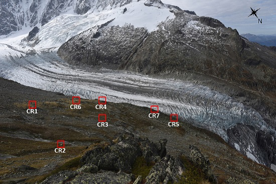
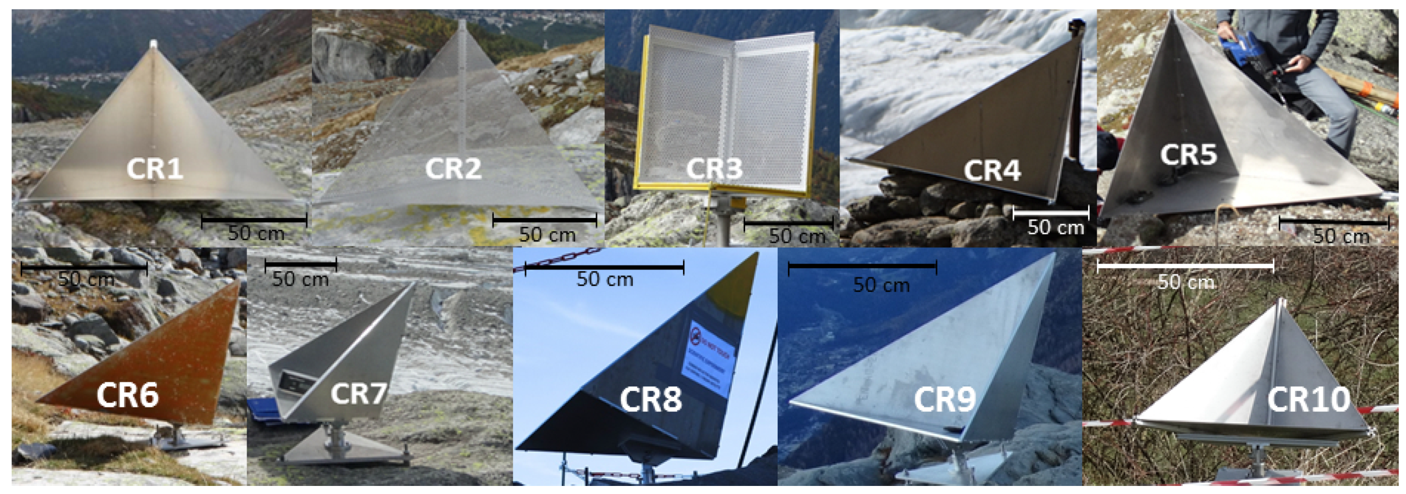
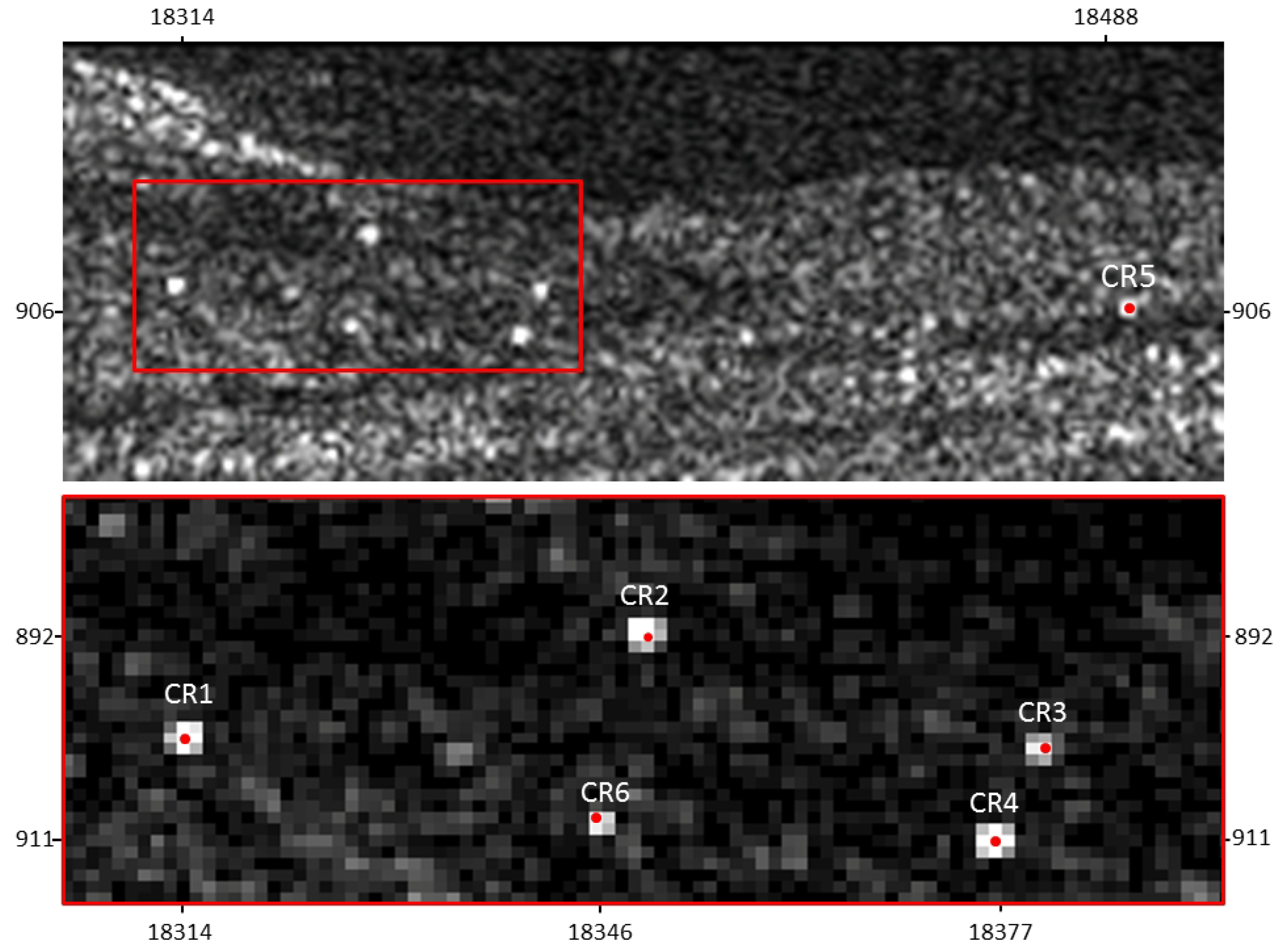
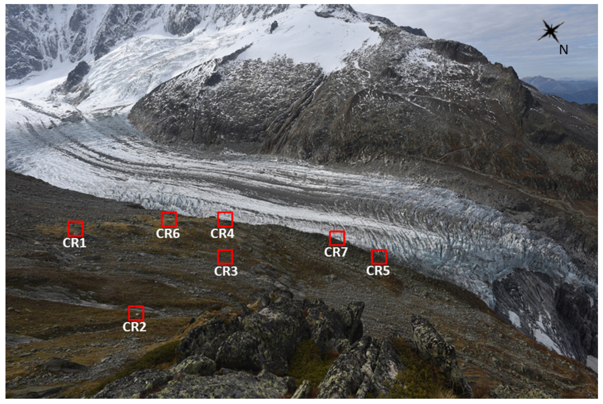
3.1.1. Identification of CRs

CRs appear as bright points in SAR images because of their strong backscattering properties. In order to determine pixels containing CRs, we used an approach based on the method of spectral correlation used for the selection of coherent scatterers [31] by taking advantage of the point-like target characteristics of a CR in each SAR acquisition. The power spectrum was evaluated for each pixel and then divided into sub-looks [32] (4 looks in range × 4 looks in azimuth) by band-pass filtering using a Kaiser window. Then, an inverse Fourier transform was carried out, giving 16 band-pass filtered SLC. Finally, the spectral correlation and the mean to sigma ratio (MSR) of the 16 band-pass filtered SLC was evaluated for each pixel. By applying restrictive threshold on the spectral correlation and on the MSR (0.6 and 1.7, respectively), pixels corresponding to CR positions were identified for all CRs installed during the two experiments in the grass field, except the smallest one (CR10, L = 450 mm). Note that the same procedure was used before the installation of CRs and no pixel was selected in the grass field. Thus, knowing the location of the CRs in the field, it is easy to verify if the selected pixels correspond to CRs or not. CR10 was identified by using the same threshold on spectral correlation but without threshold on MSR. Figure 6 shows the result obtained by this identification process for the 955 cm-side CR (CR1)on the 26 March 2016 Sentinel-1 image.

3.1.2. Signal-to-Clutter Ratio and Intensity Time Series

The potential of using a CR to get accurate displacement measurement can be estimated by analyzing its response stability in SAR image time series. For this, it is possible to estimate the Signal-to-Clutter Ratio (SCR) and the expected phase error [33]:

$$\mathsf{\Phi }err=\frac{1}{\sqrt[]{2SCR}}.$$

(4)

SCRs of the CRs were calculated in each SAR image by calculating the average clutter [4] from four diagonal windows surrounding the pixel selected by the method presented in Section 3.1.1. RCS of each CR was calculated with the method proposed in [4] by multiplying the integrated point target energy of the selected pixel by the surface of the ground range pixel spacing. Figure 7a shows the intensity, RCS and SCR of CR1 during the first stage of our experiments, from 2016-03-26 to 2016-05-13. RCS values estimated from the first image on 2016-03-26 are consistent with the theoretical values presented in Table 1. Then, the decrease of these three parameters over time is due to water accumulation. The results of the CR quality estimation of the three CRs installed in 2017 is shown in Figure 7b. RCS estimates of CR1 from the second stage of experiments, from 2017/04/20 to 201706/07, are also consistent with the theoretical values for CR1 and CR3, and RCS of CR2 is lower than the expected. CR2 has the fragile construction with perforated 2-mm-plates. The loss of RCS may be explained by the deformation/curvature of the plates following the assembly/disassembly and shipping after the measurements in the anechoic chamber. We only realized that the CR was damaged after the first experiment in Choisy. However, the curvatures were reduced before the new installation of the CR in the Argentière site. The result of the gain of the RCS is presented in

Table 2. RCS (dBm${}^2$), SCR (dB) and related phase error (rad) estimated in 2017/09/30 Sentinel-1 image.

Corner Reflectors	RCS	SCR	Phase Error
CR1	28.00	17.16	0.17
CR2	28.47	14.15	0.19
CR3	23.50	13.36	0.19
CR4	28.18	12.69	0.2
CR5	28.72	17.21	0.17
CR6	22.47	13.73	0.19

. One of the recommendations for the use of perforated CRs could be to strengthen the construction. Note that SCR of CR2 is weak, less than 9, so RCS estimation based on amplitude dispersion might not be ideal [34]. Averages of RCS and SCR are given in

Table 3. Averages of RCS (dBm${}^2$) and SCR (dB) estimated in 7 Sentinel-1 descending images, from 2017/04/20 to 2017/06/07.

Corner Reflectors	Mean RCS	Mean SCR
CR1	29.24	17.11
CR2	27.47	8.89
CR3	25.13	13.32

.

3.2. Integration of Crs in High Relief Areas

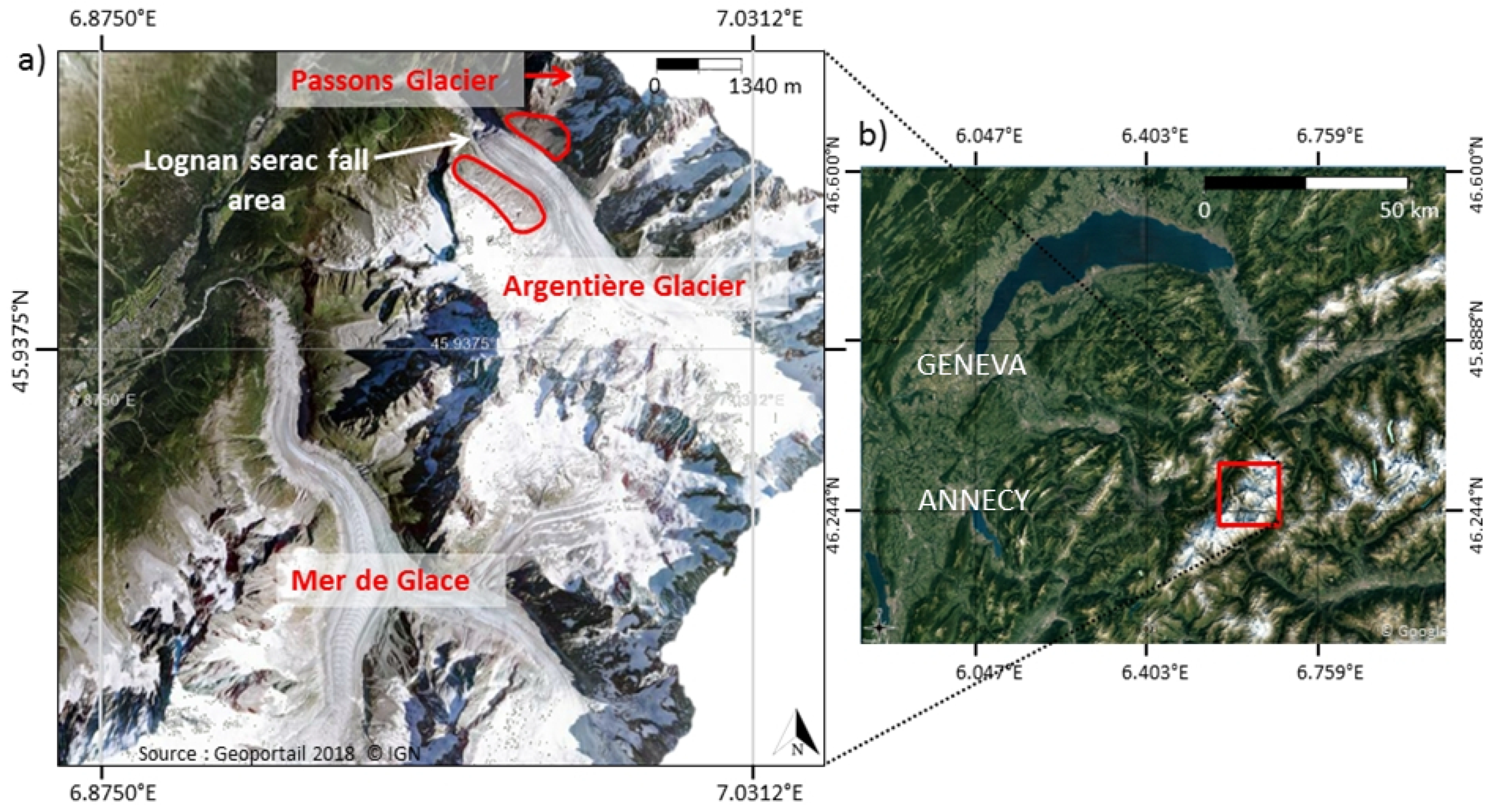
3.2.1. Chamonix–Mont-Blanc Test Site

The Mont-Blanc massif in the Western part of the Alps is a constantly used in studies to understand the local impact of global warming on glaciers [35,36,37,38]. The Mont-Blanc massif is also studied to assess inherent risks to periglacial and permafrost processes. These complex geomorphological processes lead to slope instabilities that could generate risks for the mountain territories [39,40,41]. Therefore, moraines can be affected by large scale deformations over very long time period and also by localized small scale displacements, potentially causing large unstable blocks to fall [42,43,44]. Consequently, it is crucial to develop tools that can monitor instabilities in these areas.

Two CRs were set up on the Argentière glacier (45${}^{\circ }$57${}^{\prime }$N, 6${}^{\circ }$58${}^{\prime }$E) in order to help InSAR surface displacement monitoring. The visibility of both the ascending oriented CR (CR8) and the descending oriented CR (CR9) is analyzed and a method to get precise estimation of their locations is presented.

Another interesting test area, close to the Lognan serac fall area, was chosen and is presented in this section and in Section 4.2. This area of 6 km${}^2$ is cut into two parts (circled in red in Figure 8), on both sides of the glacier. The West side is part of a ski resort and is composed of moraines from the Rognons and Argentière glaciers and other rocky slopes. The East side is composed of a lateral moraine in its lower part and rocky slopes in the upper part, which includes detritus products from Passons and Adams Reilly glaciers. Thus, this test area is likely to be affected by deformations

A total of seven CRs deployed in the East side of this area were used in this study. Five CRs (CR1, CR2, CR3, CR4 and CR5) have been deployed during the study, complementing a previous experiment with CR6 and CR7. Combining radar CR response analysis with the analysis of pictures acquired by the two cameras installed on a site overlooking the study area and dedicated to glacier monitoring (five automatic acquisitions per day) offers the possibility to link local meteorological conditions and radar response. In this way, cameras can be used to relate the signal variations observed on CR response to the meteorological conditions (snow conditions in particular). All these CRs were established for descending acquisitions because the high layover effect in ascending images due to high relief.

3.2.2. Identification of CR Pixels

The installation of the CRs on the test site was carried out in several steps. CR4 and CR5 were set up in October 2016. CR6 and CR7 were already installed, and were reoriented for Sentinel-1 data, in the same orientations as the other CRs. Then, new missions were conducted, in July for installation of CR1, and in September 2017 for installations of CR2 and CR3. In this study, we worked with several time series covering different time spans, from 10 weeks to more than one year (Figure 5, in order to estimate the visibility of each CR.

Pixels containing CRs were selected using the same method as presented in Section 3.1.1. All the CRs were successfully identified, except the CR (CR7) with a 450-mm side length. If we use less restrictive parameters (lower MSR/coherence thresholds), all the pixels with CR can be detected, but there are also pixels without CR among the selected ones. Consequently, this experiment with CR7 and the previous experiment with CR10 provided in Section 3.1 show that triangular CR with a 450-mm side length seems to be too small to be detected in Sentinel-1 images without false detection. Results of the pixel selection with one Sentinel-1 image are illustrated in Figure 9.

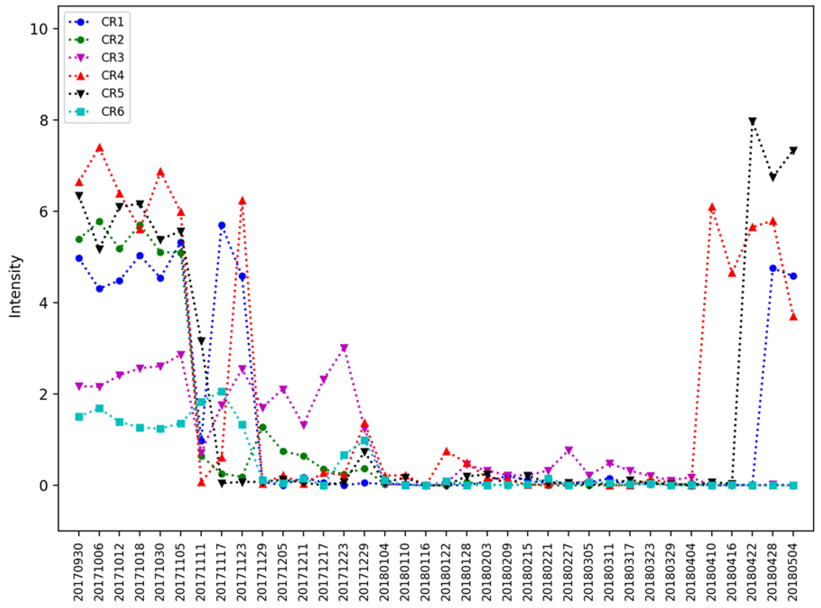
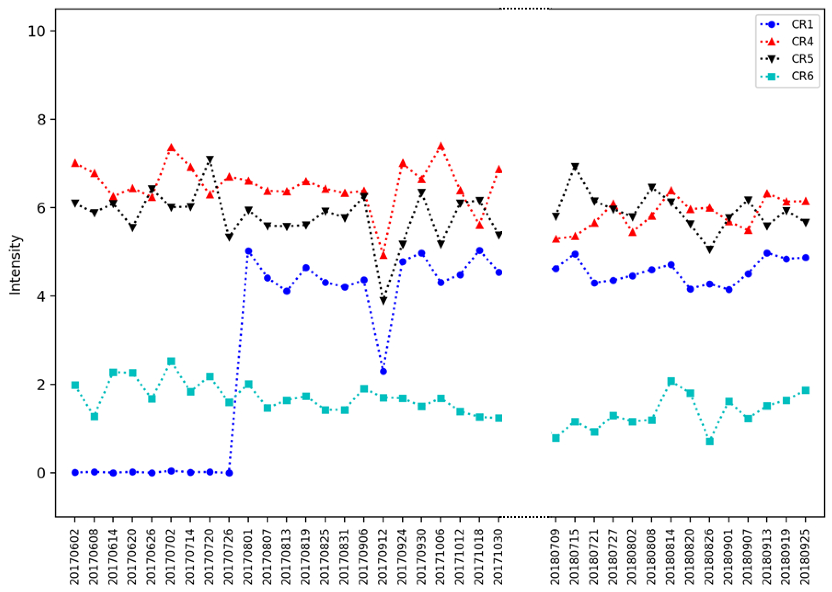
3.2.3. Intensity Analysis

Since the winter in mountainous areas is the most difficult period for surface displacement monitoring (i.e., due to snow falls), the major focus is on the period covering winter 2017–2018, when the entire network was set up, with several shapes and sizes of perforated or unperforated CRs.

An intensity analysis of pixels with CRs was performed between the end of September 2017 and the beginning of May 2018 (see Figure 10). Observation of the first acquisitions in September and October made it possible to check the highest response of each CR before winter. It shows that the pixel corresponding to CR4 had the strongest intensity. Pixels corresponding to CR3 and CR6 had the lowest intensity, which is consistent with the CR size. The drastic decrease of intensity visible on the intensity image of 2017/10/24 (see Figure 10) was due to snow falls during a period with temperature above 0 °C. Thus, the low backscattered signal in each CR (even in the perforated ones) can be explained by snow with a high wetness. Once the snow had melted, a similar event was identified with the 2017/11/11 photographs with a wet snow fall during the acquisition. However, backscatters of CR1 and CR3 recover their initial level (before the snow falls) right after in the next acquisition. This illustrates local aspects of snow evolution (wind, orientation, shaded or sunny areas, etc.). We notice that CR3 (perforated rectangular shape) is the CR whose intensity remains, roughly, stable longer than any other CR (see Figure 10). Photograph analysis between 2017/12/29 and 2018/04/04 confirmed that the snow cover decreased the radar response drastically. On 2018/04/22, snow cover was measured at 249 cm (source: meteo-ciel.com) at the ski resort of Chamonix (Lognan, 1970 m a.s.l.) located at the left margin (relative to the glacier flow direction) of the Argentière glacier and around 2 km from the test site.

Consequently, the lack of radar responses of CR2, CR3 and CR6 might be due to an important complex snow cover (several layers, wet snow) or to the degradation of the CRs settings. CR response analysis was completed at the end of September 2018 (see Figure 11). CR2 and CR3 were still invisible at the end of June. After a field inspection in September, it turned out that CR2 and CR3 were damaged. By analyzing all the available photographs, traces of avalanches observed several times near CR2 can explain the damage. CR3 was less damaged, which can be explained by a stronger construction and/or by damages caused by the weight of the snowpack. There was no more snow on the installation areas of CR2 and CR3 in the photographs from 15 June 2018, so damages had occurred between the end of December 2017 and the middle of June 2018. Conversely, CR6 became visible again after the snow melting. Considering the two damaged CRs (CR2 and CR3) and CR7 which appeared to be too small, four CRs were used for a PSI study between Summer 2017 and Summer 2018. This longer study started on 2017-07-27 after the installation of CR1 (Figure 11) up until the end of summer 2018 in order to avoid heavy snow falls. Note that low precipitation is still possible in summer, like on 2018-08-26 and 2017-09-12 (Figure 11) when low snow falls were confirmed by the photographs taken from our two monitoring cameras.

3.2.4. Stability Analysis

One of the goals of this study is to define the potential of CRs for slope and moraine monitoring with Sentinel-1 data. One way to monitor this complex environment may be a Persistent Scatterer (PS) strategy using one of the CRs as reference. In such approach, the reference point should be stable in terms of displacement, since all the results will be relative to this point. A preliminary task to multi-temporal InSAR can be a phase analysis based on the CRs’ response. Ref [45] defined a stability index as the ratio between the mean and the standard deviation of the amplitude of a SAR image in a time series. In this study, we estimated an equivalent of this index based on intensity instead of amplitude. This stability index was calculated on several Sentinel-1 SAR image time series; the results are presented in

Table 4. Intensity Mean Sigma Ratio (dB) estimated on six CRs between 2016-10-10 and 2018-09-25. Temperature and snow cover information from a weather station of Meteo France (45.97991, 6.89132, 2330 m a.s.l) on Aiguilles Rouges massif at 7 km from the CR.

Corner	2016-10-10	2017-05-15	2017-08-01/2017-10-30	2017-09-30	2018-07-09
Reflectors	2017-09-30	2017-09-06	2018-07-09/2018-09-25	2017-10-30	2018-09-25
CR1	X	X	8.86	16.35	16.56
CR2	X	X	0.47	20.16	0.85
CR3	X	X	0.49	12.60	0.95
CR4	1.76	25.35	11.09	11.19	16.79
CR5	1.45	7.18	10.66	12.54	13.95
CR6	2.89	4.89	4.34	8.66	3.44
Temperature	Positive/negative alternation	Mainly positive	Mainly positive	Positive/negative alternation	Positive
Snow cover	7 months out of 12	1 month out of 4	<30 cm, only few days	<30 cm, only few days	None

. Stability information was completed by an analysis of seasonal graphics of air temperature and snow cover depth. Snow depth evolution analysis allows detecting snow falls and snow melting periods, and temperature analysis can be used to understand snowpack evolution. These parameters are measured every two hours by the Aiguilles Rouges “Nivose” weather station of $MeteoFrance$ (the French service of meteorology and climatology). This weather station is set up at about 7 km from the test site. Its altitude (2330 m a.s.l) corresponds to the altitude of the CRs (2320 to 2435 m). A weak amplitude stability is observed during the one-year study (59 images, 2016-10-11/2017-09-30) for non-perforated CR due to high intensity variability caused by snow falls and very variable temperatures, resulting in a succession of snow accumulation and melting periods between November 2016 and May 2017. However, the stability index is high when considering the sub-time series during a period without snow falls (23 images, 2017-05-15/2017-09-06). An equivalent analysis was initiated on a time series outside winter marked by positive temperatures and without significant snow cover (37 images, 2017-08-01/2017-10-30 and 2018-07-09/2018-09-25) with perforated CRs, i.e., CR2 and CR3. Unfortunately, they were damaged in winter 2018, which explains their very low stability index. Considering that CR4 was installed on a rocky outcrop, avoiding locations susceptible to soil slope instability, and, according to stability index analysis, this CR can be considered as the best choice of reference point.

3.2.5. Signal-to-Clutter Ratio and RCS

Stability analysis was completed by a phase noise estimation based on the Signal-to-Clutter Ratio. Table 2 presents the expected phase error with the Signal-to-Clutter Ratio estimated in the same way as in Section 3.1.2. As the SCR estimated for a CR is dependent on its RCS and the influence of clutter next to it [4], and since RCS values are close to those estimated on grass field, SCR changes may mainly be linked to neighboring clutter. For instance, the SCR increased for CR2. This can be explained by a low backscattered signal of clutter next to it (see Figure 12).

The RCS values estimated from Sentinel-1 images in a high mountainous area should be close to those obtained on grass-field. The RCS estimation of CR1 is smaller than in the previous estimation. CR1 was set up with an offset of 12° in azimuth from the optimal orientation (because of field constraints), which can explain the RCS loss. The RCS of CR2 is 1 dB larger than the estimation in the grass field. Before installation, we tried to straighten one of its plates which presented a curvature. This may explain the gain of RCS. The estimated RCS value of CR3 is 1.6 dB lower than the previous estimation. Based on the anechoic chamber results, it could be due to an offset of around 5° in elevation, or around 15° in azimuth. The first hypothesis is the most likely since the inclinometer used for the set up is not very precise. CR1, CR4 and CR5 are the same size, so results are therefore consistent. In conclusion, the RCS estimates are close to those measured on the grass field. Besides the precision of the estimation method, it is challenging to identify other parameters causing RCS changes.

Table 2 shows that all CRs have an estimated phase error smaller than 0.19 rad. Thus, according to the SCR and corresponding phase error estimation, all the CRs can be used for displacement measurement with reasonable error.

4. CRs for Glacier and Moraine Monitoring

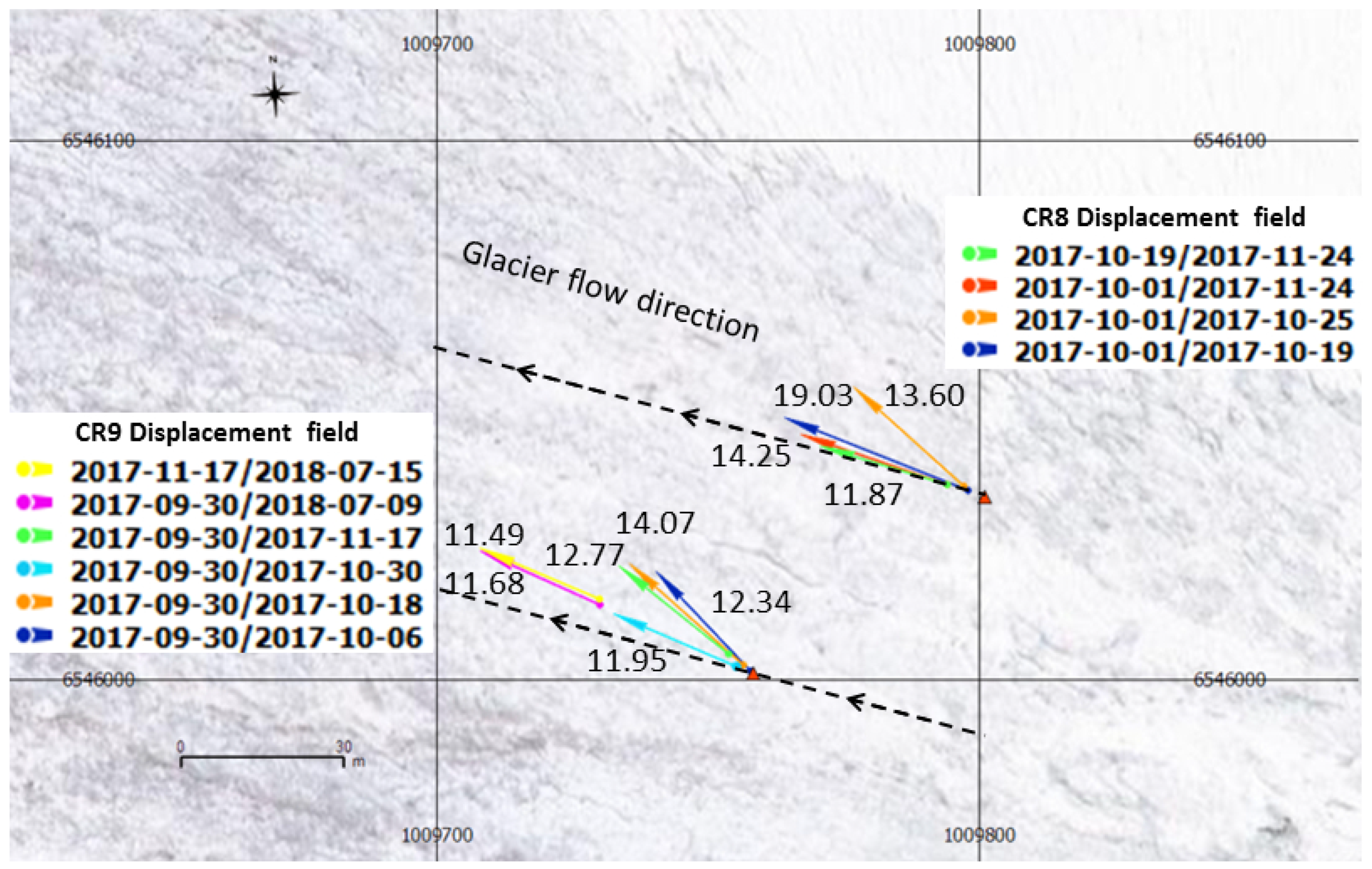
4.1. Use of CR Location for Glacier Motion Estimation

In order to track surface displacement of the Argentière glacier, two triangular CRs (CR8 and CR9), were installed on its surface (45°56${}^{\prime }$34.2${}^{″}$N, 7°00${}^{\prime }$00.4${}^{″}$E, 2677 m a.s.l.). Sentinel-1 Single Look Complex (SLC) images have a resolution between 2.7 m and 3.5 m in range and 22 m in azimuth [ESA]. In this study, image processing was done without multi-looking. We used SLC images with a pixel spacing about 2.33 m in range and 13.88 m in azimuth. Due to incidence angle of 39.7° of the radar wave, pixel spacing is around 3.6 m in ground range. With such resolution, the determination of the precise position of CRs on the ground can be challenging, in particular with the low resolution in azimuth.

A pixel selection was applied to distinguish the CR response from those of scatterers like rocks or other detritus products (method presented in Section 3.1.1). In fact, the position of of the CRs was analyzed thanks to its point-like target characteristics in each radar acquisition. By applying a threshold of $0.67$ to the spectral correlation and $1.5$ to the MSR, only two pixels were selected corresponding to the CRs for each SLC. In order to improve the ground position estimation, a sub-pixel localization was carried out by finding the maximum peak of each CR. The peak is determined by oversampling the data after performing complex fast Fourier transform (FFT). Then, a Lanczos interpolator can retrieve the peak position which is the effective phase center of the radar scatterer. In this study, the effective phase center is the apex of the reflector.

Finally, sub-pixel locations were orthorectified with a Digital Elevation Model (DEM, 5 m spacing). The position of the CRs was successfully estimated in six descending Sentinel-1 images, acquired from 2017-09-30 to 2018-07-09 and in four ascending Sentinel-1 images acquired from 2017-10-01 to 2017-11-24. Then, horizontal displacement of the CR through time was computed based on successive Easting and Northing positions in different acquisitions. To convert 2D-displacement into 3D-displacement, successive heights had to be estimated. These heights could have been obtained using DEM values relative to the CR positions. However, it could have introduced uncertainty linked to the location estimation and DEM errors. Thus, a local slope was estimated and used to convert 2D into 3D-displacement estimation. Displacement direction was computed and compared to the local glacier flow direction, corresponding to the main slope direction estimated from the DEM. Results are presented in

Table 5. Distance covered by CR8 between two successive positions and the corresponding velocity.

Dates	Time Interval (d)	Velocity (cm/d)	Direction	Difference from Glacier
				Flow Direction
2017-10-01/2017-10-19	18	$19.0$	$294.7$°E	−9.7°
2017-10-01/2017-10-25	24	$13.6$	$315.1$°E	−30.1°
2017-10-01/2017-11-24	54	$13.4$	292°E	−7.0°
2017-10-19/2017-11-24	36	$11.9$	$289.9$°	−4.9°

and

Table 6. Distance covered by CR9 between two successive positions and the corresponding velocity.

Dates	Time Interval (d)	Velocity (cm/d)	Direction	Difference from Glacier
				Flow Direction
2017-09-30/2017-10-06	6	$12.3$	$316.2$°E	−31.8°
2017-09-30/2017-10-18	18	$14.1$	$311.9$°E	−26.9°
2017-09-30/2017-10-30	30	$12.0$	$293.4$°E	−8.4°
2017-09-30/2017-11-17	48	$12.8$	$309.0$°E	−24.0°
2017-09-30/2018-07-09	282	$11.7$	$294.4$°E	9.4°
2017-11-17/2018-07-15	240	$11.5$	$293.2$°	−8.2°

and Figure 13. CR8 and CR9 were visible since their installation on 2017-09-29 and for about two months after the first significant snow falls after 2017-11-24. Once the snow melted, CR9 could be successfully identified again in two images in July 2018. Then, the response lost could be explained by a change in the CR orientation caused by ice surface ablation under warm temperature effects. Sub-pixel positions were estimated in other images (2017/10/12 and 2017/10/30 in descending images for instance), but their relative displacement directions show important deviation from the local glacier flow direction. Those results are not taken into account.

We estimated 3D velocities from the absolute location and compared the results with previous studies. The objective of this approach was to validate the potential of CRs for glacier flow monitoring without external information, except a DEM.

In [46], Sentinel-1 geolocation accuracy was studied with experiments conducted on 194 images with triangular CRs from 1 m to 1.5 m. It gave a mean error in slant range of 0.15 m and 1.44 m in azimuth. It also highlighted a subswath-dependent azimuth offset, with 4.30 m for the subswath IW1, 2.2 m for IW2 and 0.12 m for IW3. Since CR8, oriented for an ascending path, is in the sub-swath IW2 and CR9, oriented for descending path, is in IW3, we can expect better accuracy for CR9’s absolute location than that for CR8’s. For the descending path, Sentinel-1 azimuth direction is 9°E and slant range direction is 279°E. As the glacier flow main direction is about 285°E, slant range displacement is the main component of the displacement. For the ascending path, slant range direction is 81°E and azimuth direction is 351°E. Thus, a significant part of the displacement is represented by the azimuth component. Thus, we can reasonably expect more accurate results with CR9 than with CR8. Then, the longer the time interval observation is, the smaller the uncertainty of estimated velocity will be.

Velocity estimates presented in Table 5 and Table 6 are consistent with the mean displacement rate from 2007 to 2010 of 13.3 cm/day obtained by a GPS station at around 2770 m a.s.l. on Argentière glacier, quite close to CR8 and CR9 [47]. Recently, a new study based on the same GPS station gave similar velocities in 2016, with mean velocities within a range from 11 to 16 cm/day, depending on the season [48]. The mean velocity was about 12 cm/day during the period March–June, and about 11 cm/day during the period September–December. These results were used as ground truth to derive the Root Mean Square Error (RMSE) of the velocity of CR8 and CR9. It gave an RMSE of 4.4 cm/day for CR8 and 1.6 cm/day for CR9. These study results match better with CR9’s velocity results than CR8’s, confirming the assumption of a more accurate estimate in descending path than in ascending path. The maximum offset is indeed obtained on a short time interval in ascending images (2017-10-01/2017-10-19). The pairs with the smallest velocity uncertainty are obtained with CR9 (2017-09-30/2018-07-09 and 2017-11-17/2018-07-15), since they represent the longest time intervals.

Thus, corner reflectors with Sentinel-1 data can be a good tool for Glacier monitoring. However, given conditions met on a glacier, with instabilities of the CRs due to surface change during warm periods and heavy snow falls in winter, it remains challenging to get a long-term monitoring of the glacier flow.

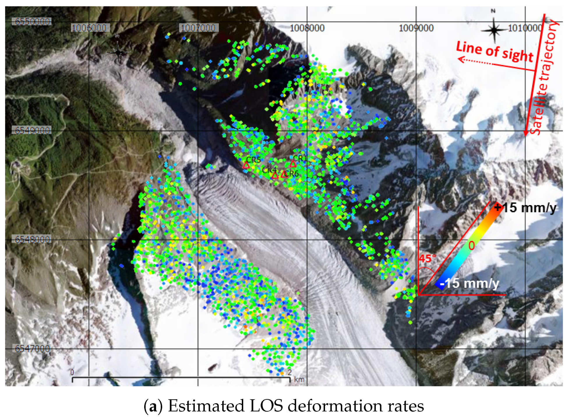
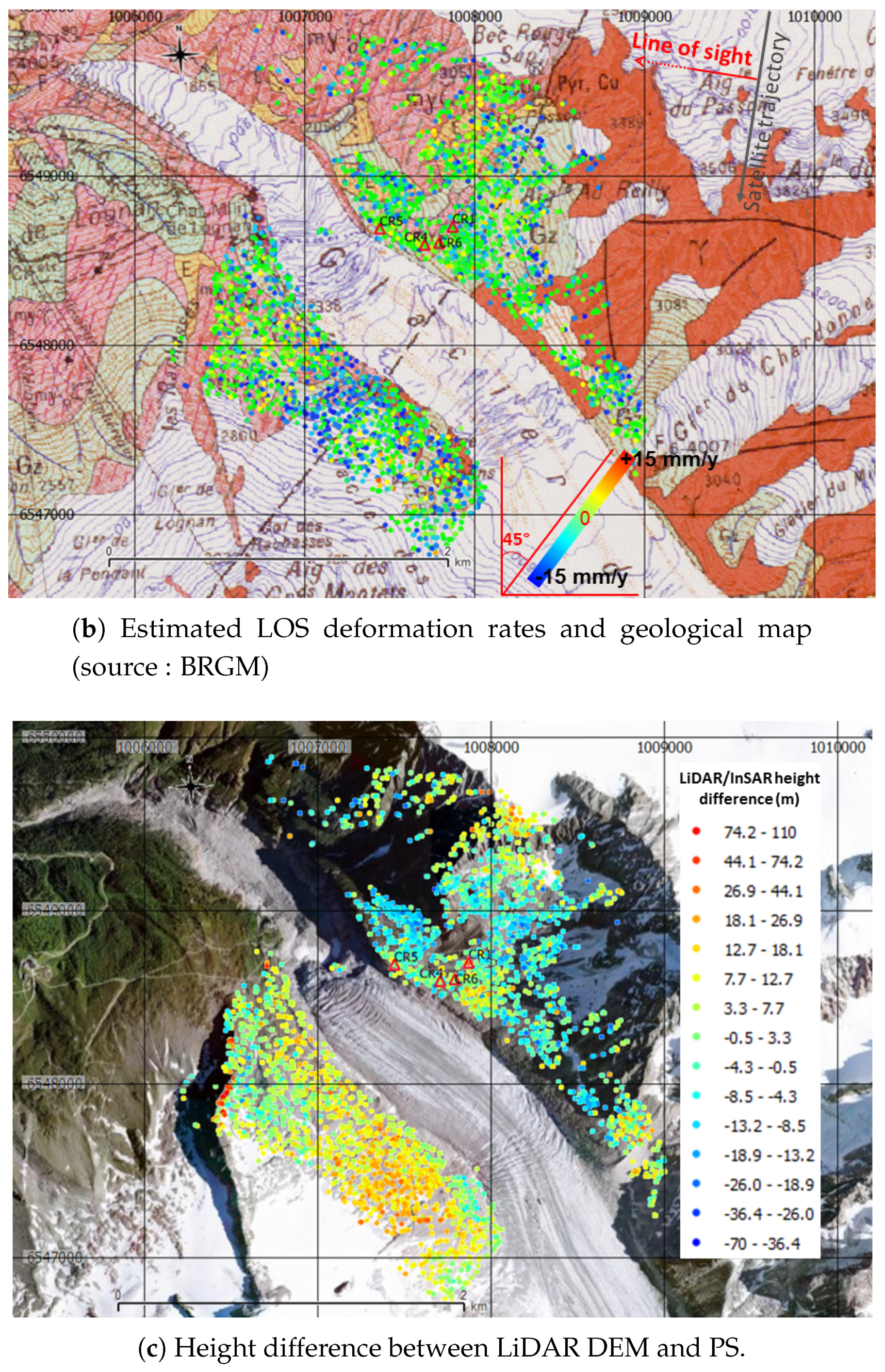
4.2. Joint Use of Crs and Psi Strategy for Estimating Moraine and Slopes Stability

A deformation analysis based on a Persistent Scatterer (PS) approach using Interferometric Point Target Analysis (IPTA) module [49] of GAMMA Software was performed on the test area presented in Section 3.2.1. The application of the PS approach in natural terrain is a challenging task because it is difficult to get a sufficient number of coherent targets as well as a point reference to estimate deformation rates. Displacement rate measurements were obtained over CRs and coherent features (rocks, low vegetation cover areas) by implementing a small network of CRs and thanks also to the presence of enough natural point targets on the moraine and surrounding slopes.

In addition to a specific data selection, another way to reduce decorrelation is to minimize the deformation phase by choosing pairs of images with reduced time interval and by including redundant observations [50]. In this study, all pairs with temporal baselines smaller or equal to 18 days were selected (i.e., a 6-day interval between acquisitions gives the pairs date 1-date 2, date 1-date 3, date 1-date 4, date 2-date 3, date 2-date 4, etc.). The stack formed by this approach is therefore called a multi-reference stack. Only the pairs with a perpendicular baseline of less than 100 meters were considered. This deformation analysis was carried out by combining a PS strategy and Small Baseline approach. In order to reduce orbital residual component, we used the highest quality precise orbit files (Precise Orbit Ephemerides).

4.2.1. Data Selection

According to the previous stability analysis in Section 3.2.4, the possible longer study with the maximum number of CRs covered 420 days, starting from 2017-08-01 to 2018-09-25. In order to minimize the temporal decorrelation due to surface change, acquisitions between 2017-10-30 and 2018-07-09 were not selected, to avoid periods with snow falls. Consequently, 27 descending Sentinel-1 images were used, spread over two periods of 90 and 83 days.

4.2.2. Radar Processing

First, the PS candidates were selected on the co-registered SLCs. Then, the interferogram stack was computed, the topographic phase based on the 5-m DEM was estimated and subtracted to get the differential interferogram stack. An iterative approach was used to estimate atmospheric phase delay and then the relative height correction, with a regression considering successively the linear phase dependence with the perpendicular baseline component and the linear phase dependence with time. Then, the phase time series was calculated by Singular Value Decomposition (SVD) to convert the multi-reference unwrapped phase into the single-reference phase time-series using a weighted least-squares approach [50]. No assumption on the displacements occurred during the gap between the two periods covered by the selected data was made. The algorithm used in the IPTA module jointly estimates the deformation phase time-series and a DEM height correction, thanks to a phase model which includes a height related term proportional to the derivative of the interferometric phase [50]. Finally, Line Of Sight (LOS) displacement and linear deformation rates were estimated considering the single reference stack.

4.2.3. Validation Method of Height Correction

In this PS approach, particular attention was paid to height correction. CR-related PS heights were compared to precise ground measurements (GPS and tacheometer). Non-CR-related PS heights were compared to LiDAR-based Digital Surface Model (DSM) acquired in June 2015. InSAR techniques give relative measurements, so height estimates are, in the same way as deformation estimates, relative with respect to a reference point [51]. Thus, using a CR with a very precise known height as a reference point prevents the propagation of shift between the extracted value and the real value of the reference point to all the PS height estimates.

For CRs’ heights and positions, the quality check is based on a comparison with CRs’ coordinates obtained by Differential GPS and tachymetry approach. A network of four GPS was used for a period of 12 h. One GPS was used as a local GPS reference, three adjusted GPS and a total station were used to measure relative positions of the CRs from the GPS network. Then, the GPS measurements were combined with the total station measurement to get refined CRs’ coordinates. Because of the height difference (up to 1100 m) between the local reference in the valley and three other GPS, the estimation accuracy is around 10–20 cm.

For non-CR-related PS, the validation of height corrections was realized with a DSM LiDAR. Note that, even with a DEM without errors, the initially extracted heights of each PS cannot be exact. These values are the result of an interpolation from a regular grid (DEM) to an irregular spaced data (height map) using multi-looking factor. While the DEM used in this study is a 5-m resolution DEM, but over-sampled in mountainous areas from a coarser resolution, the DSM LiDAR used for quality check has a resolution of 2 m. DSMs based on LiDAR data usually have vertical accuracy better than 30 cm on relatively flat terrains [52,53,54]. The mean slope on the study area is about 31°, with some parts exceeding 40°. However, the accuracy decreases for steep slopes with an RMSE of around 60 cm for slopes greater than 30° [55,56]. This allows us to use values of DSM LiDAR as ground truth data.

4.2.4. Absolute Location Error

The quality check approach proposed in this study for a non-CR PS is based on the extraction of the DSM LiDAR value at the PS position and the comparison of this value with the one obtained by PS processing chain. However, it is worth noting that height errors induce errors in solving of the Doppler-Range-Ellipsoid equations to retrieve the 3D Cartesian coordinates of the target [57]. An error in height estimate results in an error in estimating the absolute location, which in turn will condition the extracted value of the DSM LiDAR. Therefore, the value of the difference between the PS height and the LiDAR height does not represent the exact height error.

In order to limit uncertainty due to an error in the absolute positioning, we only kept the PS candidates with a successful sub-pixel estimation and rejected those not likely to be PS. Since the sub-pixel precision partly depends on the SCR value [58], the SCR was estimated on each PS with the same method presented in Section 3.1.2 and the results are discussed in Section 4.2.5. Apart from atmospheric path delay, the other sources of errors in absolute positioning, such as the azimuth shift, solid earth tides or tectonics [57,59,60,61] are not discussed in this study. Thus, a difference between PS height and LiDAR height may be due to an error in height estimation and/or due to an error in the absolute positioning.

According to [62], the PS height precision can be expressed by the height standard deviation defined as:

$${\sigma }_h=\sqrt{\frac{1}{{\left(N{\sigma }_b{}_{\perp }\right)}^2-{\left(N{\overline{b}}_{\perp }\right)}^2}}\frac{\lambda R_{0}sin\left(\theta \right)}{4\pi }.{\sigma }_{\varphi },$$

(5)

where N is the number of images, ${\overline{b}}_{\perp }$ and ${\sigma }_{b_{\perp }}$ are the mean and the standard deviation of baseline distribution, $\lambda$ the wavelength, $R_0$ the range distance, $\theta$ the incidence angle and ${\sigma }_{\varphi }$ is the standard deviation of phase. In this study, the standard deviation of baseline distribution would have been 37.0 m if all the pairs had been used. After testing several threshold on the minimum and maximum baseline selection, it appears that the standard deviation can be maximized to 48.3 m if the pairs with baseline smaller than 20 m are not used, which leads to a lower height standard deviation according to Equation (5). Note that with a single reference strategy approach, the standard deviation of baseline distribution would have been even lower with 28.3 m. Thus, the multi-reference strategy and the pair selection used here should improve the height precision.

Moreover, the standard deviation of the phase noise is defined in [62] as:

$${\sigma }_{\varphi }^2=\frac{1}{2.SCR}+{\sigma }_{atm}^2,$$

(6)

where ${\sigma }_{atm}$ is the residual atmospheric phase signal. Since CRs provide a high SCR [6], height estimation is expected to be better on CRs than on other PSs with lower SCR.

4.2.5. Processing Results

The first height correction with a simultaneous estimation of atmospheric and residual topographic phase component (called simultaneous approach in

Table 7. Height quality check.

Processing Step	PS Height Shift $\mathit{Mean}\pm \mathit{\sigma }$ (m)	PS Height RMSE ${}^{*}$ (m)	CR Height RMSE ${}^{*}$ (m)
First iteration (simultaneous atmosphere/height estimates)	$-19.5\pm 24.3$	31.1	11.01
First iteration (Stepwise approach)	$8.5\pm 12.3$	14.98	2.58
Final estimate (Stepwise approach)	$-3.0\pm 14.55$	14.85	0.15

* Root Mean Square Error.

), gives results with a mean error of −19.5 m and a standard deviation of 24.3 m. Then, we proposed to first estimate the atmospheric phase delay and then estimate the residual topographic phase component. With this approach (called stepwise approach in Table 7), the mean error is 8.5 m with a standard deviation of 12.3 m. Moreover, the mean height correction is about −25.7 m with the simultaneous approach, and about −2.7 m with the stepwise approach. Thus, it turns out that height estimations in the simultaneous approach are overestimated. After an iterative process of height and atmosphere corrections, a Singular Value Decomposition (SVD) based Least-Squares inversion was performed to convert the multi-reference stack phases into a single reference time series. This inversion, presented in Section 4.2.2 and described in [50], combines an estimation of the deformation phase time-series and estimation of a DEM height correction, giving a final height estimate.

A quality check was made with DSM LiDAR heights; results are presented in Table 7. It turns out that the mean difference between the final PS heights and the LiDAR heights were successfully reduced. The height RMSE on CR1, CR5 and CR6 is 0.15 m. According to [63], the PS height precision of Sentinel-1 is around 5 m. Our study shows that the mean precision can be improved with a specific approach and the use of CRs gives very good height estimation. The absolute position precision was studied by computing the shift with respect to the GPS measurements, giving an RMSE of 0.83 m in 2D and 0.84 m in 3D. In comparison, an RMSE of 0.42 m in 3D was obtained with 44 ENVISAT images and two 1-m CRs, after timing correction (bistatic offset, atmospheric phase delay, solid earth tides...) and calibration offsets estimation [61]. Thus, with fewer images and without complete timing correction, the results of our study seems to be reasonable.

Finally, deformation rate was estimated on 4202 PSs, including 3835 with a temporal MSR above 1.5. Figure 14a shows that areas without PS-like scatterers correspond to areas with vegetation cover or very steep terrains on the right edge of the Argentière glacier due to shadow areas in the radar images. An unstable area was identified on the left edge of the glacier with deformation rates exceeding −10 mm/year (Figure 14a). It turns out that this area corresponds to a geologic contact identified as a fault (see Figure 14b) called Faille de l’Angle (BRGM, French National Geological Services). The differences between the final PS heights and the LiDAR heights are presented in Figure 14c. The outliers, represented in red in Figure 14c, correspond to a vertical ridge, where a small positioning error leads to a very strong height error. More generally, differences are more significant on the right side of the glacier than on the left side. This is mainly explained by higher values of SCR for the scatterers on the left edge. For instance, a threshold of 20 dB to the SCR value results in a height RMSE of 9.7 m, with 1265 PSs, almost all located on the left side of the glacier. The RMSE can reach 5.34 m with a threshold of 30 dB, but only 54 PSs remain. In the area close to the fault, 95% of the selected pixels have a SCR larger than 20 dB with a maximal difference with LiDAR height of 19.9 m, which can result of a maximal error in LOS displacement of 3 mm.

5. Conclusions

In this paper, the benefit of using CRs with Sentinel-1 data is presented in the context of glacier motion and moraine instability monitoring. The RCS of three different models of CRs (triangular, perforated triangular and perforated rectangular) were measured in an anechoic chamber. The visibility and the performance of 10 CRs were investigated in a grass field, on a glacier, on slopes and a moraine in a mountainous area. Experiments allowed linking their visibility with meteorological conditions, tracking a glacier displacement and estimating slope instabilities. On one hand, the use of perforated plates doesn’t introduce a significant loss of RCS compared to the traditional plates, for both triangular and rectangular CRs, in both C-band and X-band; on the other hand, it shows the importance of a precise assembly without space between the plates and with a cut as precise as possible. RCS measurements in the anechoic chamber show that rectangular CRs can be recommended for small displacements monitoring, where ground displacements do not disrupt their elevation angles. As this shape optimizes the RCS in optimal settings, it could be useful in quite strong backscattering areas with restrictions on the choice of the CR size, in urban areas for instance. In contrast, if there is no limitation on the CR size, the stability of triangular CR represents a great interest for any type of displacement monitoring.

CRs should be big enough for them to be distinguished from other strong scatterers. In this study, a 45-cm-side-length triangular CR seems to be too small for Sentinel-1 C-band images. Snow falls in the one-year time series decreased the stability index drastically. This motivated us to work on a subset time series of 27 Sentinel-1 images without snow fall. The SCR, and the effective phase error, smaller than 0.19 rad., were calculated for each CR on each SAR image. Displacement monitoring in winter in an Alpine context remains a challenging task. The use of a perforated CR on the installation site exposed to the wind and snow falls can help maintain the CRs’ visibility. However, heavy snow falls and complex snow layers with wet snow cancel the CRs’ contribution from the radar backscattering. It could be interesting to cover the CR with plastic to limit the accumulation of snow. However, the snowpack was exceptionally deep during the winter 2017/2018 (more than four meters), and each CR would have been covered by the snow.

Glacier motion detection was conducted by means of a precise evaluation of the CR positions. The results with these two CRs in four Sentinel-1 images acquired in an ascending path and in seven images in a descending path, present velocity relevant to previous GPS studies on the Argentiìere glacier. Displacement rates achieved with a time interval longer than 24 days are between 11 and 14 cm/day, which are in agreement with displacement rates of 13.3 cm/day obtained from 2007 to 2010 by a GPS station [47] and recent results based on the same GPS station with mean horizontal velocities within a range from 11 to 16 cm/day [48].

The results of an ad hoc PSI processing on the moraines and the surrounding slopes of the Argentière glacier demonstrate the potential of the joint use of CRs and PSI processing in measuring slope instabilities. The presence of CRs for visibility and stability tests in summer has provided the opportunity to use a stable CR as reference point. The proposed approach makes it possible to obtain height estimation on CRs with an RMSE of 0.15 m. The height precision on non-CR PSs was also analyzed. Despite the limited available number of images due to presence of snow, the mean height difference with a precise LiDAR-based DSM is around 3.0 m. Furthermore, this approach has made it possible to identify an unstable area which seems to be related to the presence of the geological fault.

References

1. Joughin, I.; Smith, B.E.; Abdalati, W. Glaciological advances made with interferometric synthetic aperture radar. J. Glaciol. 2010, 56, 1026–1042. [Google Scholar] [CrossRef]
2. Barboux, C.; Strozzi, T.; Delaloye, R.; Wegmüller, U.; Collet, C. Mapping slope movements in Alpine environments using TerraSAR-X interferometric methods. ISPRS J. Photogramm. Remote Sens. 2015, 109, 178–192. [Google Scholar] [CrossRef] [Green Version]
3. Sarabandi, K.; Tsen-Chieh, C. Optimum corner reflectors for calibration of imaging radars. IEEE Trans. Antennas Propag. 1996, 44, 1348–1361. [Google Scholar] [CrossRef]
4. Garthwaite, M. On the Design of Radar Corner Reflectors for Deformation Monitoring in Multi-Frequency InSAR. Remote Sens. 2017, 9, 648. [Google Scholar] [CrossRef]
5. Groot, J.; Otten, M. SAR Imaging of Corner Reflectors Larger Than the Spatial Resolution. IEEE Trans. Geosci. Remote Sens. 1994, 32, 721–724. [Google Scholar] [CrossRef]
6. Parker, A.L.; Featherstone, W.E.; Penna, N.T.; Filmer, M.S.; Garthwaite, M.C. Practical Considerations before Installing Ground-Based Geodetic Infrastructure for Integrated InSAR and cGNSS Monitoring of Vertical Land Motion. Sensors 2017, 17, 1753. [Google Scholar] [CrossRef]
7. Freeman, A. SAR calibration: An overview. IEEE Trans. Geosci. Remote Sens. 1992, 30, 1107–1121. [Google Scholar] [CrossRef]
8. Doöring, B.; Schrank, D.; Schwerdt, M.; Bauer, R. Absolute Radiometric Calibration of TerraSAR-X—Approach and Ground Targets. In German Microwave Conference; VDE: Berlin, Germany, 2008; pp. 1–4. [Google Scholar]
9. Bovenga, F.; Pasquariello, G.; Pellicani, R.; Refice, A.; Spilotro, G. Landslide monitoring for risk mitigation by using corner reflector and satellite SAR interferometry: The large landslide of Carlantino (Italy). CATENA 2017, 151, 49–62. [Google Scholar] [CrossRef]
10. Schlögel, R.; Thiebes, B.; Mulas, M.; Cuozzo, G.; Notarnicola, C.; Schneiderbauer, S.; Crespi, M.; Mazzoni, A.; Mair, V.; Corsini, A. Multi-Temporal X-Band Radar Interferometry Using Corner Reflectors: Application and Validation at the Corvara Landslide (Dolomites, Italy). Remote Sens. 2017, 9, 739. [Google Scholar] [CrossRef]
11. Qin, Y.; Perissin, D. Monitoring Ground Subsidence in Hong Kong via Spaceborne Radar: Experiments and Validation. Remote Sens. 2015, 7, 10715–10736. [Google Scholar] [CrossRef] [Green Version]
12. Rohmer, J.; Loschetter, A.; Raucoules, D.; de Michele, M.; Raffard, D.; Le Gallo, Y. Revealing the surface deformation induced by deep CO2 injection in vegetated/agricultural areas: The combination of corner-reflectors, reservoir simulations and spatio-temporal statistics. Eng. Geol. 2015, 197, 188–197. [Google Scholar] [CrossRef]
13. Trouvé, E.; Pétillot, I.; Bolon, P.; Bombrun, L.; Cotte, N.; Hajnsek, I. Monitoring Alpine glacier activity by a combined use of TerraSAR-X images and continuous GPS measurements—The Argentière glacier experiment. In Proceedings of the 7th European Conference on Synthetic Aperture Radar, Friedrichshafen, Germany, 2–5 June 2008. [Google Scholar]
14. Zhu, W.; Zhang, Q.; Ding, X.; Zhao, C.; Yang, C.; Qu, F.; Qu, W. Landslide monitoring by combining of CR-InSAR and GPS techniques. Adv. Space Res. 2014, 53, 430–439. [Google Scholar] [CrossRef]
15. Algafsh, A.; Inggs, M.; Mishra, A.K. The effect of perforating the corner reflector on maximum radar cross section. In Proceedings of the 2016 16th Mediterranean Microwave Symposium (MMS), Abu Dhabi, UAE, 14–16 November 2016; pp. 1–4. [Google Scholar]
16. Parizzi, A.; Perissin, D.; Prati, C.; Rocca, F. Artificial Scatterers for SAR Interferometry. In Proceedings of the 2005 Dragon Symposium (SP-611), Santorini, Greece, 29 June–1 July 2005; Volume 46, p. 27. [Google Scholar]
17. Qin, Y.; Perissin, D.; Lei, L. The Design and Experiments on Corner Reflectors for Urban Ground Deformation Monitoring in Hong Kong. Int. J. Antennas Propag. 2013, 2013, 1–8. [Google Scholar] [CrossRef]
18. Garthwaite, M.C.; Lawrie, S.; Dawson, J.; Thankappan, M. Corner Reflectors as the Tie Between InSAR and GNSS Measurements: Case Study of Resource Extraction in Australia. FRINGE 2015, 731. [Google Scholar] [CrossRef]
19. Gray, A.; Vachon, P.; Livingstone, C.; Lukowski, T. Synthetic aperture radar calibration using reference reflectors. IEEE Trans. Geosci. Remote Sens. 1990, 28, 374–383. [Google Scholar] [CrossRef]
20. Polycarpou, A.C.; Balanis, C.A.; Tirkas, P.A. Radar Cross Section of Trihedral Corner Reflectors: Theory and Experiment. Electromagnetics 1995, 15, 457–484. [Google Scholar] [CrossRef]
21. Ruck, G.T.; Barrick, D.E.; Stuart, W.D.; Krichbaum, C.K. Radar Cross Section Handbook; Plenum Press: New York, NY, USA, 1970; Volumes 1 & 2. [Google Scholar]
22. Doerry, A.W. Reflectors for SAR Performance Testing; Sandia Report, SAND2008-0396; Sandia National Laboratories: Albuquerque, CA, USA, 2008.
23. Doerry, A.W.; Brock, B.C. Radar Cross Section of Triangular Trihedral Reflector with Extended Bottom Plate; Sandia Report, SAND2009-2993; Sandia National Laboratories: Albuquerque, CA, USA, 2009.
24. Zhou, Z.; Yan, H.; Yin, H. High Frequency RCS Representation of Trihedral Corner Reflectors with Scalene Triangle Aperture. In Proceedings of the 2015 IEEE 12th International Conference on Ubiquitous Intelligence and Computing and 2015 IEEE 12th International Conference on Autonomic and Trusted Computing and 2015 IEEE 15th International Conference on Scalable Computing and Communications and Its Associated Workshops (UIC-ATC-ScalCom), Beijing, China, 10–14 August 2015; pp. 1621–1625. [Google Scholar]
25. Chuah, B.K.C.H.T. Modeling of RF absorber for application in the design of anechoic chamber. Prog. Electromag. Res. 2003, 43, 273–285. [Google Scholar]
26. Dun, G. Modelisation et optimisation de chambres anechoiques pour applications CEM. Ph.D. Thesis, ENSTB, Université de Bretagne occidentale, Brest, France, 2007. [Google Scholar]
27. Zink, M.; Kietzmann, H. Next Generation SAR—External Calibration; German Aerospace Center (DLR): Köln, Germany, 1995; p. 45. [Google Scholar]
28. Robertson, S.D. Targets for Microwave Radar Navigation. Bell Syst. Tech. J. 1947, 26, 852–869. [Google Scholar] [CrossRef]
29. Guillemot, T.; Pottier, E.; Saillard, J.; Levrel, J.; Lebreton, E. Determining the far-field RCS from the response to a cylindrical wavefront. Aerosp. Sci. Technol. 1997, 1, 215–223. [Google Scholar] [CrossRef]
30. Knott, E.F. Radar Cross Section Measurements; VanNostrand Reinhold: New York, NY, USA, 1993. [Google Scholar]
31. Schneider, R.; Papathanassiou, K.; Hajnsek, I.; Moreira, A. Polarimetric and interferometric characterization of coherent scatterers in urban areas. IEEE Trans. Geosci. Remote Sens. 2006, 44, 971–984. [Google Scholar] [CrossRef]
32. Henry, C.; Souyris, J.; Marthon, P. Target detection and analysis based on spectral analysis of a SAR image: A simulation approach. In Proceedings of the 2003 IEEE International Geoscience and Remote Sensing Symposium, Toulouse, France, 21–25 July 2003; Volume 3, pp. 2005–2007. [Google Scholar]
33. Adam, N.; Kampes, B.E.M. Development of a Scientific Permanent Scatterer System: Modifications for Mixed ERS/Envisat Time Series. In Proceedings of the 2004 Envisat & ERS Symposium (ESA SP-572), Salzburg, Austria, 6–10 September 2004. [Google Scholar]
34. Ketelaar, G.; Marinkovic, P.; Hanssen, R. Validation of Point Scatterer Phase Statistics in Multi-Pass INSAR. In Proceedings of the 2004 Envisat & ERS Symposium (ESA SP-572), Salzburg, Austria, 6–10 September 2004. [Google Scholar]
35. Rabatel, A.; Letréguilly, A.; Dedieu, J.P.; Eckert, N. Changes in glacier equilibrium-line altitude in the western Alps from 1984 to 2010: Evaluation by remote sensing and modeling of the morpho-topographic and climate controls. Cryosphere 2013, 7, 1455–1471. [Google Scholar] [CrossRef]
36. Gardent, M. Glacier Inventory and Retreat of French Alpine Glaciers since the End of Little Ice Age. Ph.D. Thesis, Université de Grenoble, Grenoble, France, 2014. [Google Scholar]
37. Le Roy, M.; Nicolussi, K.; Deline, P.; Astrade, L.; Edouard, J.L.; Miramont, C.; Arnaud, F. Calendar-dated glacier variations in the western European Alps during the Neoglacial: The Mer de Glace record, Mont Blanc massif. Quat. Sci. Rev. 2015, 108, 1–22. [Google Scholar] [CrossRef]
38. Rabatel, A.; Sanchez, O.; Vincent, C.; Six, D. Estimation of Glacier Thickness From Surface Mass Balance and Ice Flow Velocities: A Case Study on Argentière Glacier, France. Front. Earth Sci. 2018. [Google Scholar] [CrossRef]
39. Deline, P.; Gardent, M.; Magnin, F.; Ravanel, L. Morphodynamics of the Mont Blanc massif (European Alps) in a changing cryosphere. In Proceedings of the 9th EGU General Assembly, Vienna, Austria, 22–27 April 2012. [Google Scholar]
40. Ravanel, L.; Deline, P.; Lambiel, C.; Duvillard, P. Stability Monitoring of High Alpine Infrastructure by Terrestrial Laser Scanning. IAEG XII Congress. 2014, 1, 169–172. [Google Scholar]
41. Magnin, F.; Josnin, J.Y.; Ravanel, L.; Pergaud, J.; Pohl, B.; Deline, P. Modelling rock wall permafrost degradation in the Mont Blanc massif from the LIA to the end of the 21st century. Cryosphere 2017, 11, 1813–1834. [Google Scholar] [CrossRef] [Green Version]
42. Blair, R.W. Moraine and Valley Wall Collapse due to Rapid Deglaciation in Mount Cook National Park, New Zealand. Mount. Res. Dev. 1994, 14, 347. [Google Scholar] [CrossRef]
43. Mortara, G.; Chiarle, M. Instability of recent moraines in the Italian Alps. Effects of natural processes and human intervention having environmental and hazard implications. G. Geol. Appl. 2005, 1, 139–146. [Google Scholar]
44. Hugenholtz, C.H.; Moorman, B.J.; Barlow, J.; Wainstein, P.A. Large-scale moraine deformation at the Athabasca Glacier, Jasper National Park, Alberta, Canada. Landslides 2008, 5, 251–260. [Google Scholar] [CrossRef]
45. Bovenga, F.; Refice, A.; Pasquariello, G.; Nitti, D.O.; Nutricato, R. Corner reflectors and multi-temporal SAR interferometry for landslide monitoring. In Proceedings of the SPIE Remote Sensing 2014 Conference, Amsterdam, The Netherlands, 22–25 September 2014. [Google Scholar]
46. Schubert, A.; Miranda, N.; Geudtner, D.; Small, D. Sentinel-1A/B Combined Product Geolocation Accuracy. Remote Sens. 2017, 9, 607. [Google Scholar] [CrossRef]
47. Ponton, F.; Walpersdorf, A.; Gay, M.; Trouvé, E.; Mugnier, J.L.; Fallourd, R.; Cotte, N.; Ott, L.; Serafini, J. GPS and TerraSARX time series measure temperate glacier flow in the Mont Blanc massif (France): The Argentière glacier test site. In Proceedings of the European Geosciences Union General Assembly 2012 (EGU 2012), Vienna, Austria, 22–27 April 2012. [Google Scholar]
48. Garnier, R. Suivi des variations du glissement du glacier d’Argentière par GPS haute fréquence. Master’s Thesis, Institut des sciences de la terre (ISTerre), Université Grenoble Alpes, Gières, France, 2017. [Google Scholar]
49. Werner, C.; Wegmuller, U.; Strozzi, T.; Wiesmann, A. Interferometric point target analysis for deformation mapping. In Proceedings of the 2003 IEEE International Geoscience and Remote Sensing Symposium, Toulouse, France, 21–25 July 2003. [Google Scholar]
50. Werner, C.L.; Wegmüller, U.; Strozzi, T. Deformation Time-Series of the Lost-Hills Oil Field using a Multi-Baseline Interferometric SAR Inversion Algorithm with Finite Difference Smoothing Constraints. In AGU Fall Meeting Abstracts; American Geophysical Union: Washington, DC, USA, 2012. [Google Scholar]
51. Kampes, B.M. Radar Interferometry: Persistent Scatterer Technique; Number 12 in Remote Sensing and Digital Image Processing; Springer: Dordrecht, The Netherlands, 2006. [Google Scholar]
52. Maune, D.F. Digital Elevation Model Technologies and Applications: The Dem Users Manual, 2nd ed.; ASPRS: Bethesda, MD, USA, 2007. [Google Scholar]
53. Liu, X.; Zhang, Z.; Peterson, J.; Chandra, S. LiDAR-Derived High Quality Ground Control Information and DEM for Image Orthorectification. GeoInformatica 2007, 11, 37–53. [Google Scholar] [CrossRef] [Green Version]
54. Aguilar, F.J.; Mills, J.P. Accuracy assessment of lidar-derived digital elevation models. Photogramm. Rec. 2008, 23, 148–169. [Google Scholar] [CrossRef]
55. Hodgson, M.E.; Bresnahan, P. Accuracy of Airborne Lidar-Derived Elevation. Photogramm. Eng. Remote Sens. 2004, 70, 331–339. [Google Scholar] [CrossRef]
56. Takahashi, T.; Yamamoto, K.; Senda, Y.; Tsuzuku, M. Estimating individual tree heights of sugi (Cryptomeria japonica D. Don) plantations in mountainous areas using small-footprint airborne LiDAR. J. For. Res. 2005, 10, 135–142. [Google Scholar] [CrossRef]
57. Montazeri, S.; Rodriguez Gonzalez, F.; Zhu, X.X. Geocoding Error Correction for InSAR Point Clouds. Remote Sens. 2018, 10, 1523. [Google Scholar] [CrossRef]
58. Dheenathayalan, P.; Small, D.; Schubert, A.; Hanssen, R.F. High-precision positioning of radar scatterers. J. Geod. 2016, 90, 403–422. [Google Scholar] [CrossRef] [Green Version]
59. Gernhardt, S. High Precision 3d Localization and Motion Analysis of Persistent Scatterers Using Meter-Resolution Radar Satellite Data. Ph.D. Thesis, Technical University of Munich, Munich, Germany, 2011. [Google Scholar]
60. Yang, M.; Dheenathayalan, P.; Chang, L.; Wang, J.; Lindenbergh, R.; Liao, M.; Hanssen, R. High-precision 3D geolocation of persistent scatterers with one single-Epoch GCP and LIDAR DSM data. In Proceedings of Living Planet Symposium 2016; Ouwehand, L., Ed.; European Space Agency: Paris, France, 2016; Volume SP-740, p. 398. [Google Scholar]
61. Dheenathayalan, P.; Small, D.; Hanssen, R.F. 3-D Positioning and Target Association for Medium-Resolution SAR Sensors. IEEE Trans. Geosci. Remote Sens. 2018, 56, 6841–6853. [Google Scholar] [CrossRef]
62. Bovenga, F.; Belmonte, A.; Refice, A.; Pasquariello, G.; Nutricato, R.; Nitti, D.O.; Chiaradia, M.T. Performance Analysis of Satellite Missions for Multi-Temporal SAR Interferometry. Sensors 2018, 18, 1359. [Google Scholar] [CrossRef]
63. Costantini, M.; Malvarosa, F.; Minati, F.; Trillo, F.; Vecchioli, F. Complementarity of high-resolution COSMO-SkyMed and medium-resolution Sentinel-1 SAR interferometry: Quantitative analysis of real target displacement and 3D positioning measurement precision, and potential operational scenarios. In Proceedings of the 2017 IEEE International Geoscience and Remote Sensing Symposium (IGARSS), Fort Worth, TX, USA, 23–28 July 2017; pp. 4602–4605. [Google Scholar]
Figure 1. Illustration of nine triangular trihedral Corner Reflectors (CRs) and one rectangular trihedral CR (CR3) used in the experimentations.
Remotesensing 11 00988 g001
Figure 2. Geometry and adjustment of a triangular CR. Ψ represents the elevation angle, θ the azimuth angle, Φ the off-nadir angle, ϕ the incidence angle, β the tilt angle and L the smaller side length of isosceles right triangular plates.
Remotesensing 11 00988 g002
Figure 3. Radar cross-section (RCS) measurements of CR1, CR2 and CR3 in an anechoic chamber. (a) RCS measurements of CR1 and (b) RCS measurements of CR2. Blue: optimal elevation angle. Red: +5 degrees, Grey: +7, Yellow: +10. (c) RCS measurements of CR3. Blue: optimal elevation angle. Red: +5 degrees, Grey: +10, Yellow: +13. Dark blue: +15, Green: +20.
Remotesensing 11 00988 g003
Figure 4. RCS measurements of CR1, CR2 and CR3 in C-band (top) and X-band (bottom). Blue: CR1, Orange: CR2, Grey: CR3.
Remotesensing 11 00988 g004
Figure 5. Summary of the number of Sentinel-1 SAR images processed on the Choisy test site (grass field) and the Argentière test site (mountainous area and glacier) with an overview of the use of CRs. The CRs used in each time series are represented by symbols proportional to their size.
Remotesensing 11 00988 g005
Figure 6. Detection of 955 cm-side CR (CR1) in Sentinel-1 descending image—Intensity image on 2016-03-26.
Remotesensing 11 00988 g006
Figure 7. Intensity, RCS and SCR estimated in Sentinel-1 data.
Remotesensing 11 00988 g007
Figure 8. (a) map showing Argentière and Mer de Glace glaciers; (b) overview map showing location of Chamonix–Mont-Blanc test site.
Remotesensing 11 00988 g008
Figure 9. Sentinel-1 intensity image (2017/09/30) in radar Doppler geometry centered on six CRs installed over a surrounding moraine of the Argentière glacier. Red points: selected pixels, red rectangle: zoom on the five closest CRs.
Remotesensing 11 00988 g009
Figure 10. SAR image intensity time series in winter 2017–2018 over six CRs installed in the study area.
Remotesensing 11 00988 g010
Figure 11. SAR image intensity time series in summer over four CRs installed in the study area.
Remotesensing 11 00988 g011
Figure 12. Photograph from one of the two cameras (Latitude: 45.97170570, longitude: 6.97575317, altitude: 2611.78) overlooking the study area (2017/09/29). Red squares: CR positions.
Remotesensing 11 00988 g012
Figure 13. Displacement vectors based on absolute location estimation of CR8 (ascending) and CR9 (descending). Color arrows indicate the orientation and the magnitude of the displacement (rates are indicated in black (cm/day)). The origin of the color arrows indicate the position of the CR at the end of each analyzed time intervals (4 for CR8, 6 for CR9). The glacier flow direction, i.e., the main slope direction, is indicated by black dashed arrows. Background image source: geoportail.gouv.fr.
Remotesensing 11 00988 g013
Figure 14. Deformation rates, geologic and height difference maps. The line of sight direction in indicated by a red arrow. The colorbar used for deformation rates is tilted so that the angle with the vertical corresponds to the incidence angle of 45°.
Remotesensing 11 00988 g014aRemotesensing 11 00988 g014b