A Partition Modeling for Anthropogenic Heat Flux Mapping in China

1
College of Resource Environment and Tourism, Capital Normal University, Beijing 100048, China
2
Institute of Remote Sensing and Geographic Information System, School of Earth and Space Science, Peking University, Beijing 100871, China
*
Author to whom correspondence should be addressed.
Remote Sens. 2019, 11(9), 1132; https://0-doi-org.brum.beds.ac.uk/10.3390/rs11091132
Submission received: 15 April 2019
/
Revised: 6 May 2019
/
Accepted: 9 May 2019
/
Published: 12 May 2019
(This article belongs to the Section Urban Remote Sensing)
Abstract
:Anthropogenic heat (AH) generated by human activities has a major impact on urban and regional climate. Accurately estimating anthropogenic heat is of great significance for studies on urban thermal environment and climate change. In this study, a gridded anthropogenic heat flux (AHF) estimation scheme was constructed based on socio-economic data, energy-consumption data, and multi-source remote sensing data using a partition modeling method, which takes into account the regional characteristics of AH emission caused by the differences in regional development levels. The refined AHF mapping in China was realized with a high resolution of 500 m. The results show that the spatial distribution of AHF has obvious regional characteristics in China. Compared with the AHF in provinces, the AHF in Shanghai is the highest which reaches 12.56 W·m−2, followed by Tianjin, Beijing, and Jiangsu. The AHF values are 5.92 W·m−2, 3.35 W·m−2, and 3.10 W·m−2, respectively. As can be seen from the mapping results of refined AHF, the high-value AHF aggregation areas are mainly distributed in north China, east China, and south China. The high-value AHF in urban areas is concentrated in 50–200 W·m−2, and maximum AHF in Shenzhen urban center reaches 267 W·m−2. Further, compared with other high resolution AHF products, it can be found that the AHF results in this study have higher spatial heterogeneity, which can better characterize the emission characteristics of AHF in the region. The spatial pattern of the AHF estimation results correspond to the distribution of building density, population, and industry zone. The high-value AHF areas are mainly distributed in airports, railway stations, industry areas, and commercial centers. It can thus be seen that the AHF estimation models constructed by the partition modeling method can well realize the estimation of large-scale AHF and the results can effectively express the detailed spatial distribution of AHF in local areas. These results can provide technical ideas and data support for studies on surface energy balance and urban climate change.
1. Introduction
Intensive human activities produce large amounts of anthropogenic heat (AH) released into the atmosphere. A large amount of AH emissions will increase the urban heat island effect. Ichinose et al. found that the AH emissions increased the heat island intensity by 1–1.5 °C in Tokyo [1]. Fan and Sailor showed that AH emissions in Philadelphia can make the heat island intensity increase 2–3 °C in a winter night [2]. The increase of temperature will have a series of effects on surface energy conversion and the atmospheric boundary layer [3,4], and further affect local air quality [5]. Young et al. investigated the effects of anthropogenic heat on ozone air quality during the summer in the Seoul metropolitan area. The release of anthropogenic heat was found to increase O3 concentration by 3.8 ppb in the urban area [5]. Hence, accurately estimating anthropogenic heat is of great significance for the urban heat island, surface energy conversion, and climatic and environmental researches.
Anthropogenic heat flux (AHF) refers to the amount of anthropogenic heat emission (AHE) generated per unit time and unit area [6]. Many researchers have carried out studies on the estimation of AHF, which generally includes three types of methods: (1) energy balance equation; (2) building energy modeling; (3) the energy-consumption inventory approach [7,8,9]. The estimation accuracy of the energy balance equation approach is highly dependent on the estimation accuracy of the parameters in the model, including sensible heat, latent heat, and storage heat [10,11]. Furthermore, an additional issue of the energy balance equation approach is that it relies on flux measurements that are not available for most locations. The building energy modeling, as its name suggests, only considers the heat emissions from buildings [12].
The energy-consumption inventory approach is employed to estimate AHF based on socio-economic data and various types of energy-consumption data, which takes into account the heat released from industry, building, and transportation [6,13,14,15]. The energy consumption from different emission sources are converted into anthropogenic heat, respectively, through a certain energy conversion experience coefficient, thus achieving an AHF estimation [1,16,17,18,19]. Since the socio-economic data and energy consumption data are based on administrative division units, the energy-consumption inventory approach can only obtain the mean value of AHF on the spatial scale represented by the statistical data, which cannot show the fine spatial pattern of AHF in the unit. What is more, it is time-consuming and laborious to obtain the complete and detailed socio-economic data and energy-consumption data for large-scale AHF estimations. Thus, it is essential and meaningful to collect the appropriate grid data and comprehensively use the multi-source remote sensing data to construct the AHF estimation model to obtain the gridded AHF data quickly and efficiently, which can better express the spatial difference of AHF inside the municipal administrative divisions.
Nighttime light (NTL) data have a unique advantage in monitoring urbanization and human activities. The brightness of nighttime light can well reflect the spatial distribution of economic activities and energy consumption [20,21,22]. There is a high linear correlation between the brightness of nighttime light and AH emission [23,24,25,26]. Yang et al. [27] estimated the AHF in China from 1992 to 2010 using the defense meteorological satellite program’s operational linescan system (DMSP/OLS) NTL data. Moreover, Ma et al. [28] obtained the gridded AHF data in Zhejiang province in China based on DMSP/OLS NTL data. However, DMSP/OLS NTL data presented a serious pixel saturation phenomenon in the urban center, which to some extent led to an underestimation of the AHF in the area. Dong et al. [14] developed a top-down method for estimating global anthropogenic heat emission based on the global radiance-calibrated DMSP/OLS NTL data, which can effectively avoid the serious pixel saturation phenomenon and LandScan 2013 global population database. The AHF results with a high resolution of 1 km were acquired in 2013. However, the characteristics of anthropogenic heat emission may be different due to the differences in regional development levels and climatic conditions. There are some limitations in the same consideration of AHF emission characteristics of all regions in the large-scale AHF estimation. Therefore, it is necessary and meaningful to carry out research on the method of AHF estimation.
In addition, some researchers have analyzed the availability of some indexes in estimating AHF to obtain more refined AHF data. For example, the AHF estimation model was established using human settlement index (HSI) [29] to realize the estimation of gridded AHF [28,30]. HSI is constructed according to the strong negative correlation between vegetation index and surface impervious data [29,31]. Although it has achieved good results in the current applications of small- and medium-scale AHF estimation, its promotion and application in large-scale areas still needs further analysis and discussion. Moreover, Zhang et al. [32] used the vegetation index to correct the nighttime light index and proposed the vegetation adjusted NTL urban index (VANUI), which uses vegetation signals to reduce NTL data saturation and increase the spatial variability of nighttime lightness values. Chen et al. characterized the spatiotemporal dynamics of anthropogenic heat flux in Beijing–Tianjin–Hebei region in China between 1995 and 2015 using the VANUI index [33]. The applicability of VANUI in estimating the gridded AHF for a large area requires further analysis and comparison.
This study aims to realize the fine gridded AHF estimation and mapping with a high resolution of 500 m in China in the year 2016. Considering the different characteristics of anthropogenic heat emission caused by the differences in regional development levels, this study adopts the partition modeling method for the first time to construct an AHF estimation model of sub-regions for better estimating the AHF in China. First, the socio-economic data and energy consumption data are used to estimate the AHF of the municipal (state, district, league) administrative regions in China based on the energy-consumption inventory approach. Next, taking the multi-source remote sensing data as independent variables, such as Suomi-NPP/VIIRS (Suomi national polar-orbiting partnership visible infrared imaging radiometer suite) NTL data which has a larger brightness range and can effectively overcome the pixel saturation phenomenon of DMSP/OLS data and MODIS (moderate resolution imaging spectroradiometer) data, and the AHF values obtained by the energy-consumption inventory approach as dependent variables, the gridded AHF estimation models are constructed in eight sub-regions respectively. Then, the performance and accuracy of different estimation models are analyzed and compared, and the optimal set of models are determined as the estimation scheme to achieve the AHF estimation in China. Finally, the refined AHF mapping with a resolution of 500 m was realized in China based on the model.
2. Data and Study Area Division
Socio-economic data and energy consumption data were derived from statistical yearbooks issued by the national bureau of statistics and local bureau of statistics [34]. Although data of Tibet autonomous region was not collected, and the statistical indicators of data in Hong Kong, Macao, and Taiwan were slightly different, a total of 308 prefecture-level (state, district, league) socio-economic data and energy consumption data were collected. Meanwhile, the data inspection and preprocessing were carried out. For the missing data, the data was allocated according to the same type of index, or estimated by the linear regression method to ensure the integrity and reliability of the data used for modeling.
Multi-temporal MODIS NDVI (normalized difference vegetation index) (MOD13A1) data were downloaded from the United States Geological Survey (USGS) [35]. The MOD13A1 product is 16-day synthetic data with a spatial resolution of 500 m. Data from April to October in 2016 were collected. A total of 28 scene images were covered in the whole country, which were re-projected from sinusoidal projection to Albers projection, and preprocessed successively by mosaicing and clipping. Then, quality control was performed according to the QC (quality control) subset of the MOD13A1 product to obtain applicable and high-quality data.
Suomi-NPP/VIIRS (national polar-orbiting partnership visible infrared imaging radiometer suite) NTL data were available at the National Oceanic and Atmospheric Administration (NOAA) [36]. The Suomi-NPP/VIIRS annual synthetic NTL data in 2016 were obtained, which have been subjected to stray light, moonlight removal processing, and background noise suppression processing. The Suomi-NPP/VIIRS NTL data were finally re-projected to the Albers projection and the resample was completed based on the nearest neighbor method.
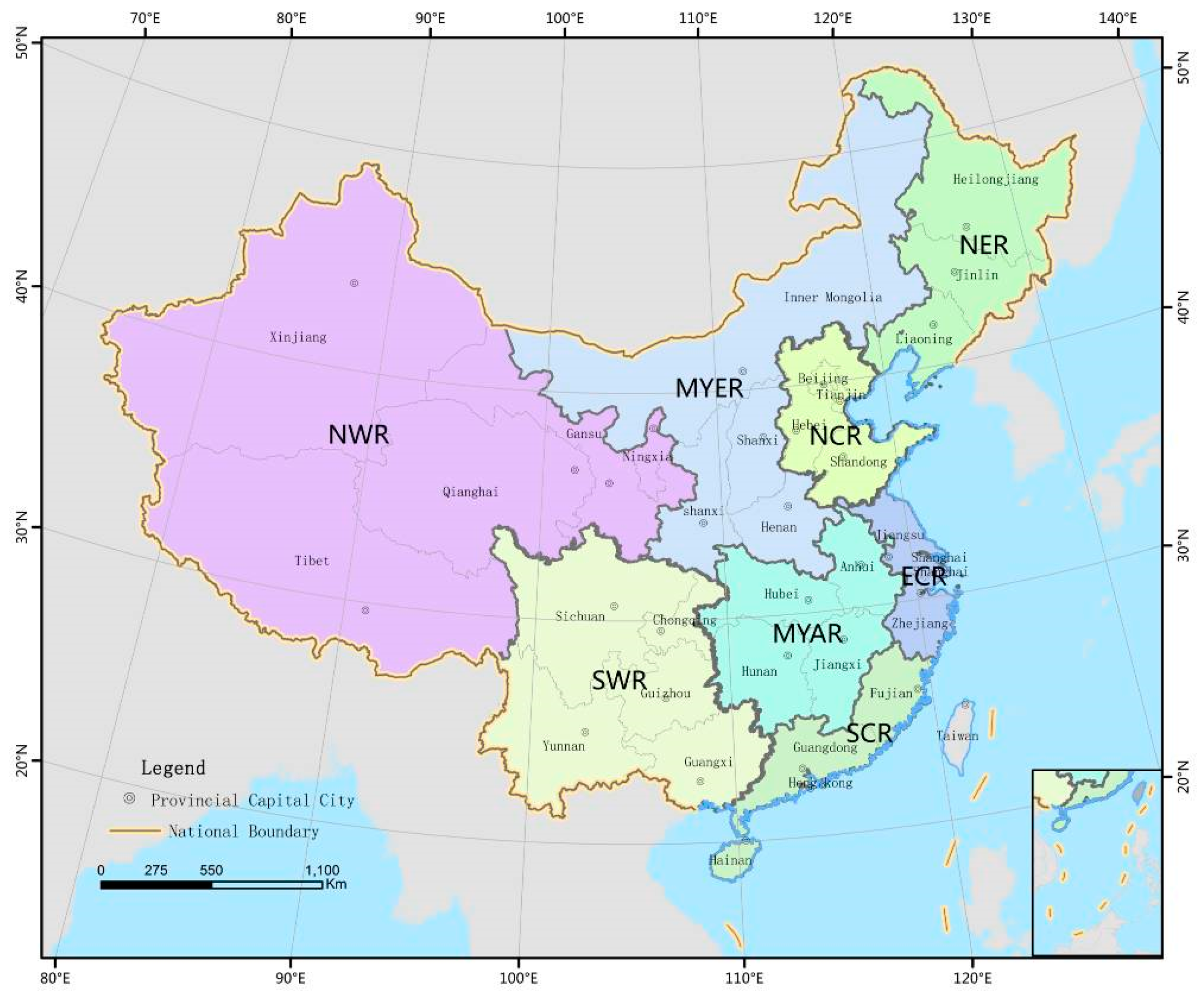
Due to the obvious regional differences in population distribution and economic development level in China, there are also large differences in the regional anthropogenic heat emissions. In order to better carry out the AHF estimation study in China, the whole study area was divided into eight sub-regions [37]. The AHF estimation was carried out in each sub-region separately. The division of the sub-regions is shown in Figure 1.
3. Methodology and Procedure
3.1. Estimation of AHF of Administrative Unit
On the basis of different emission sources of heat, the heat released from industry, transportation, buildings, and human metabolism were taken into account [6,13]. The total AHF is the sum of the four parts. The equation is:
where QS is the total AHF (W·m−2), QI is the industry heat flux (W·m−2), QB is the building heat flux (W·m−2), QV is the transportation heat flux (W·m−2), and QM is the human metabolism heat flux (W·m−2).
Heat released from industry is mainly derived from various types of energy consumption (such as coal, oil, gas, electricity, etc.). First, the energy consumption data of provinces are counted. Next, according to the national energy conversion standard coal reference coefficient, the actual energy consumption is converted into standard energy consumption, so as to obtain the total energy consumption of the province. The total energy consumption of the province is allotted based on the ratio of the secondary industry to obtain the industry energy consumption of prefecture-level cities. Further combined with the standard coal heat, the heat from industry of provinces and prefecture-level cities is obtained. The equation is:
where EI is industry consumption (unit: 10,000 tons of standard coal, tce); C is the standard coal heat, which is 29307 kJ/kg according to the national energy conversion standard; A is land area (unit: m2); T is one year.
Buildings were divided into commercial buildings and residential buildings according to functions and purposes of use. The energy-consumption (such as heat, electricity, coal, petroleum, gas, natural gas) from retail, wholesale, accommodation, living, and catering was acquired from the energy balance sheet in the statistical yearbook of provinces. The commercial buildings’ heat was allotted based on the ratio of the tertiary industry in prefecture-level cities. The residential buildings heat was allotted based on the ratio of the population in prefecture-level cities. The equation is:
where EBR and EBC are residential and commercial building consumption, respectively (unit: tce).
The consumption of gasoline and diesel in the process of driving will generate heat emissions. The energy consumption from transportation is calculated according to the sum of civilian vehicle ownership in a prefecture-level city in the economic statistics. According to Grimmond [16], heat released from transportation is calculated according to indicators, such as vehicle driving distance and fuel consumption. The equation is:
where D is the driving distance per vehicle (unit: km); V is the sum of civilian vehicles; E is combustion efficiency (unit: L/km); ρ is combustion density (unit: kg/L); NHC is the net heat combustion (unit: kJ/g).
Heat released from human metabolism was calculated based on a previous research method [18]. A day is divided into an active state and sleeping state. The period of active state is from 7:00 to 23:00, and the metabolic rate is 171 W per person. The period of sleeping state is from 23:00 to 7:00, with a metabolic rate of 70 W per person. Combined with the total population of the prefecture-level city, the heat from human metabolism is calculated:
where t1 is the sleeping hours, t2 is the active hours; P1 is the metabolic rate in sleeping state, P2 is the metabolic rate in active state;N is the sum of the population.
3.2. Construction of the Gridded AHF Partition Estimation Model
Firstly, the normalization was conducted for NDVI and NTL data based on the linear membership function, transforming the datasets into a 0 to 1 scale.
where, xmax, xmin represent the maximum and minimum pixel values, respectively. xi is the value of pixel i. is the normalized value of pixel i.
The VANUI and HSI are calculated respectively based on the normalized NDVI and NTL data:
where NDVImax is the maximum value of the multi-temporal normalized vegetation index, and NTLnor is normalized NTL data.
On this basis, the mean values of VANUI, HSI, and NTLnor in a prefecture-level (state, district, league) administrative region are calculated:
where is the index (VANUI, HSI, NTLnor) value of pixel i. is the mean value of the index in the prefecture-level city. n is the sum of pixels in the prefecture-level city.
Secondly, the regression relationship between mean AHF and is established by the statistical regression method: .
The coefficient of determination (R2) is applied to evaluate the estimated performance of the model:
where is the average value of AHF, and AHF* is the estimated value of AHF calculated by the estimation model. is the coefficient of determination of sub-region k (northern coastal region (NCR), eastern costal region (ECR), southern coastal region (SCR), northeast region (NER), middle Yellow River region (MYER), middle Yangtze River region (MYAR), southwest region (SWR), northwest region (NWR)).
The goodness of fit between VANUI, NTLnor, and AHF were compared and analyzed to explore whether VANUI could improve the correlation with AHF. Meanwhile, based on the goodness of fit results between the HSI and AHF, the applicability of the HSI for a large-scale AHF estimation is further verified.
Finally, the gridded AHF partition estimation models of sub-regions are constructed by integrating the results with high goodness of fit, so as to realize the AHF estimation:
where IDXi is the index value of pixel i; is the fitting function of sub-region k.
3.3. Procedure of the Gridded AHF Estimation Scheme
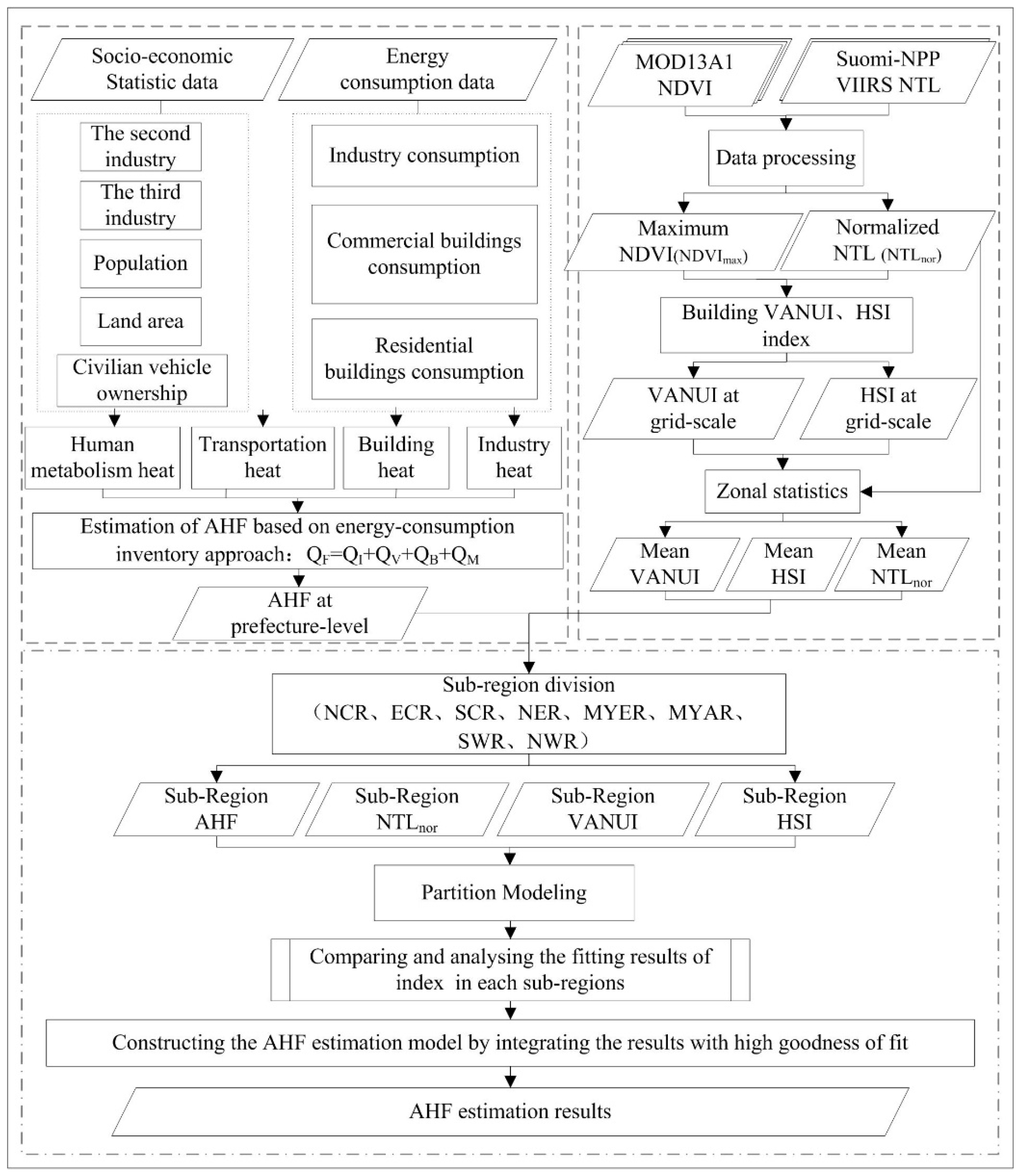
The technical process of AHF estimation is shown in Figure 2. Firstly, using the energy-consumption inventory approach, the annual total AHE and mean AHF at the provincial and prefectural levels in the year 2016 are estimated based on the socio-economic data and energy-consumption data in the different emission sources of heat (industry, building, transportation, and human metabolism). Secondly, NTL data and MODIS NDVI data are used to construct the indexes (VANUI, HSI), and the average values of the indexes in the prefecture-level city (state, district, and league) are calculated. Next, the statistical regression analysis is conducted on AHF and mean values of index in the sub-regions. The correlativity between AHF and indexes are fitted to obtain the AHF estimation models. Further, the applicability of indexes in a large-scale AHF estimation is analyzed and compared. On this basis, the AHF partition estimation models are established by integrating the results with higher goodness of fit in the sub-regions. Finally, the fine gridded AHF mapping in China is accomplished based on the model.
4. Results and Analysis
4.1. AHF Value of the Provinces
The estimated results of AHE and AHF in the provincial administrative units in 2016 are shown in Figure 3. It can be seen that:
- There are great differences in the quantity of AHE values in provinces, as shown in Figure 3a. In provinces, AHE in Shandong province is the highest which reaches 1.41 × 10¹⁹ J, accounting for 10.17% of the country’s total AHE, followed by Guangdong, Jiangsu, and Hebei. The total AHE of the four provinces account for 31.9% of the country’s total AHE. On the other hand, from the perspective of emission sources, the proportions of energy consumption from industry, building, transportation, and human metabolism are quite different in provinces. For example, the total AHE in Beijing is not high. The main emission source of heat is transportation, accounting for 37% of the total AHE in Beijing. The total AHE in Guangdong province is relatively high, and its main source of heat is industry, accounting for 62% of the total AHE in Guangdong.
- Comparing the AHF of the provinces, it can be seen from Figure 3b that the AHF value in Shanghai is the highest due to its relatively small land area, which reaches 12.56 W·m−2, followed by Tianjin, Beijing, and Jiangsu. The AHF values reach 5.92 W·m−2, 3.35 W·m−2, and 3.10 W·m−2, respectively.
4.2. The Gridded AHF Partition Estimation Model
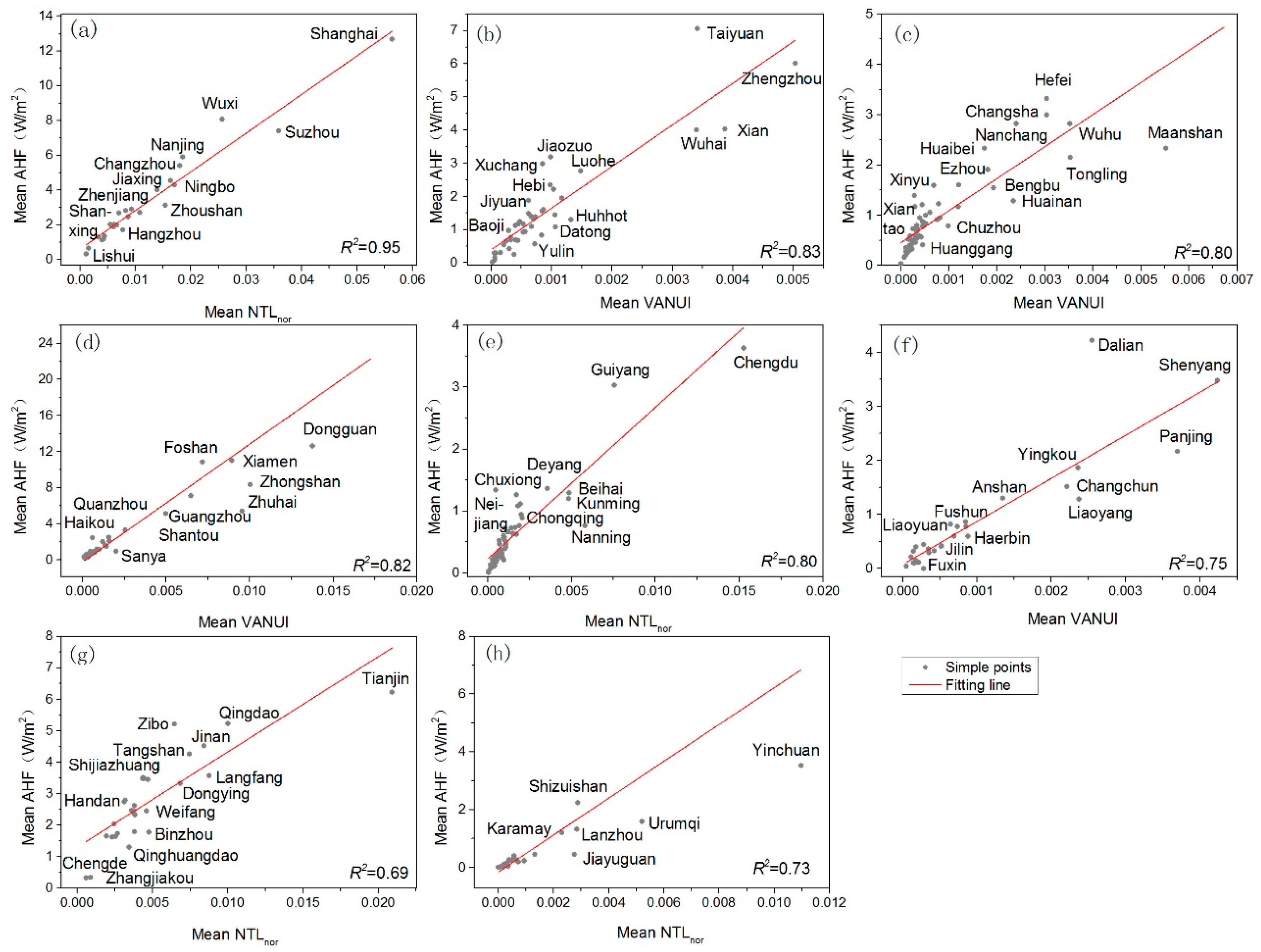
Taking AHF as the dependent variable y, and VANUI (or NTLnor) as the independent variable x, the gridded AHF partition estimation models are established. The mean AHF and VANUI (or NTLnor) of all prefecture-level cities (state, district, league) are used as sample data for linear regression analysis in the sub-regions. Part of the regression analysis results are shown in Figure 4. It can be seen that:
- The mean VANUI (or NTLnor) in sub-regions are significantly correlated with the mean value of AHF, where the range of fitting R2 is from 0.63 to 0.95.
- In the fitting results of MYER, MYAR, NER, and SCR, the fitting R2 value of VANUI data are higher than that of NTLnor data. In view of the two different estimation methods, it is necessary to make a comparison and analysis, and select the optimal fitting function as the gridded AHF partition estimation models.
Finally, the gridded AHF partition estimation models are determined by selecting the fitting results of the VANUI and NTLnor with high goodness of fit in sub-regions. The AHF estimation models and goodness of fit in sub-regions are shown in Table 1. It can be seen that the goodness of fit of the VANUI in the sub-regions of MYER, MYAR, SCR, and NER are higher than that of NTLnor. While the goodness of fit of NTLnor in other sub-regions (ECR, SWR, NCR, NWR) are higher than that of the VANUI.
4.3. The Gridded AHF Mapping Results
Based on the gridded AHF partition estimation models, the refined AHF mapping in China with a spatial resolution of 500 m is completed, as shown in Figure 5. Through qualitative and quantitative analysis, it is found that:
- On the basis of the AHF in the administrative division unit obtained based on the energy-consumption inventory approach, and further combining the indexes derived from multi-source remote sensing data, the AHF with a fine gridded scale is obtained. The result has high spatial heterogeneity, which can intuitively show the intensity and spatial characteristics of AHF inside administrative division units.
- In southwest and northwest China, the AHF values are relatively low, ranging from 0 to 5 W·m−2. The high-value AHF clusters are mainly distributed in north China, east China, and south China, especially in the Beijing–Tianjin–Hebei region, the Yangtze River delta, and the Pearl River delta. The high-value AHF in urban areas reaches 50–200 W·m−2. AHF in some urban centers is higher than 200 W·m−2. For example, the maximum AHF in Shenzhen reaches 267 W·m−2.
4.4. Validation and Analysis of the AHF Results
4.4.1. Validation of AHF Estimation Results
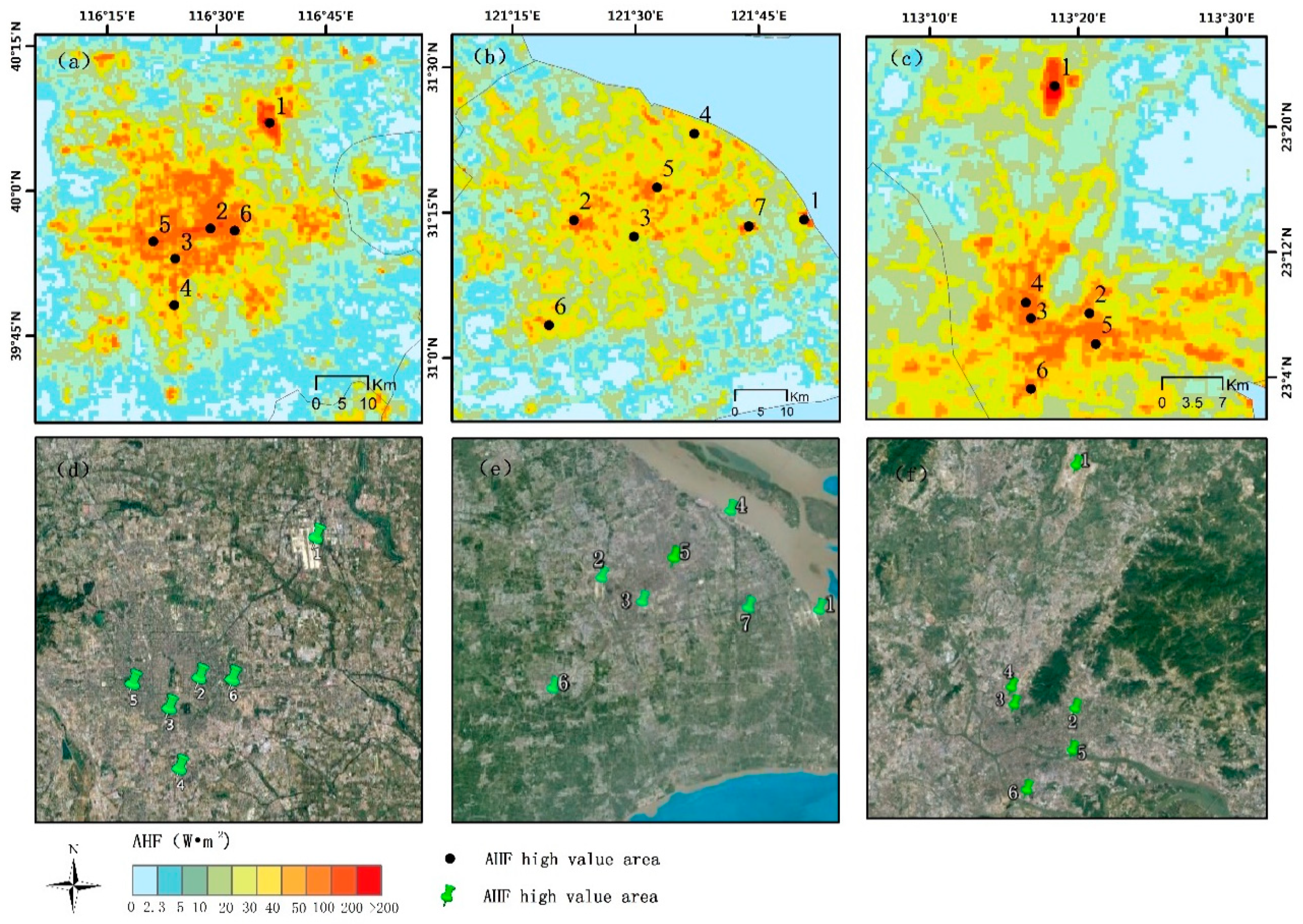
Taking Beijing, Shanghai, and Guangzhou as examples (Figure 6), combined with the regional characteristics of the city, it can be seen that the AHF estimation results in this study can effectively express the spatial characteristics of AHF in regions. Combined with a high-resolution remote sensing image (as shown in Figure 6a–f), the high-value AHF areas are mostly distributed in airports, railway stations, industry areas, and commercial centers which are typical high-energy consumption and high population centers, resulting in a large number of AH emissions. This result shows the effectiveness of the AHF estimation results in expressing the detailed distribution of AHF in local areas.
At present, the sensible heat and latent heat caused by human activities cannot be completely distinguished, and it is difficult to validate the AHF results according to field measurement data [6,30]. Therefore, the results are usually verified by comparing with previous similar studies. Due to the inconsistency in data sources and modeling methods, there is often no absolute comparability between the study results, but it can be used as reference data to verify the rationality of research results as a whole. Chen et al. [39] used energy consumption data to study the relationship between climate forcing caused by anthropogenic heat emission and population and energy consumption in China from 1978 to 2008, and obtained AHF results. Xie et al. [40] estimated the spatial distribution of AHF in China from 1990 to 2010 based on energy consumption data and gridded population data. Part of the estimation results of AHF in the prefectural level of the two existing studies and the prefectural level AHF in this study, calculated based on the obtained fine gridded AHF, are listed in Table 2.
The AHF estimation results in this study are basically consistent with the two existing research results on the order of magnitude. The result values are slightly higher than these two studies. It may be caused by the research methods and systematic errors, or from the increase of AHF over time. For example, the population and economic growth in provinces in recent years, as well as the increased energy consumption, led to the increase of the AHF.
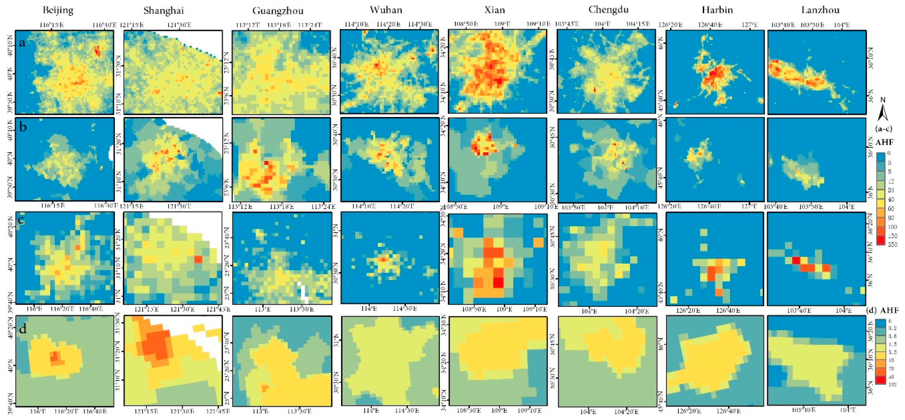
Furthermore, the AHF result with 500 m spatial resolution obtained by this study is resampled to 1 km resolution and 2.5 arc-min resolution, respectively, to compare with the AHF result of 1 km resolution obtained by the large scale urban consumption of the energy (LUCY) model [41,42] and the AHF results of 2.5 arc-min resolution obtained by Flanner et al. [43]. The heat emission from buildings, traffic, and human metabolism is considered in the LUCY model based on the energy-consumption inventory method. The energy consumption data and high-resolution population density data were employed to obtain AHF results with 1 km spatial resolution based on LUCY model [44,45]. Flanner et al. employed the energy consumption from non-renewable sources (coal, petroleum, natural gas, and nuclear) and population density data to achieve the estimation of an annual-mean gridded AHF from 2006 to 2040 [43]. A typical region was selected from eight partitions for comparison of AHF in the year 2016 respectively, as shown in Figure 7.
Comparing the AHF results of each partition, it can be seen that the AHF results in this study have higher spatial heterogeneity than the AHF results by the LUCY and Flanner model, which can better characterize the emission characteristics of AHF in regions, as shown in Figure 7. In addition, the high-value AHF and its spatial range can be better reflected. Taking Beijing as an example, combining Figure 6 and Figure 7, it can be seen that the high AH emission in airports is not well expressed in the LUCY model, and the maximum AHF in Beijing is 138 W·m−2. The results of this study show that AH emission in some places in Beijing is as high as 200–300 W·m−2, which is more significant in typical areas such as airports and train stations. The AHF values in Flanner’s model are mostly concentrated in the range of 1.5–20 W·m−2, and the expression of high-value AHF is not obvious. Overall, the AHF partition estimation scheme proposed in this study obtained good AHF estimation results.
4.4.2. Analysis of AHF Estimation Results
Taking the sub-regions of NCR, SCR, and ECR as examples, the contribution rates of AHF in different grades to the overall AHF are analyzed (as shown in Table 3). It can be seen that:
- In the NCR, the contribution rate of the AHF grade of 0–10 W·m−2 to the overall AHF is the highest, reaching 51.79%. The lowest contribution is the AHF grade greater than 100 W·m−2 with a contribution rate of 0.89%. There is a wide variation in percentage between grades. The contribution rate of AHF grade of 0–10 W·m−2 in SCR and ECR is 24.21% and 37.39%, respectively, and the contribution rate of AHF greater than 100 W·m−2 is 2.52% and 0.29%, respectively.
- On the whole, the changing range of AHF contribution rates in different grades is as follows: NCR > ECR > SCR. The difference of the AHF contribution rate in the NCR is the greatest, indicating that AHF in different grades is not evenly distributed, followed by the ECR. The difference of the contribution rate in the SCR is relatively small, indicating that AHF in different grades is more evenly distributed, and it also reflects there are relatively more high-value AHF areas within the region.
5. Discussion
5.1. Applicability of HSI for Large-Scale AHF Estimation
HSI has achieved good results in the estimation of medium-scale and small-scale AHF [28,30], but its application in estimating large-scale AHF still needs to be analyzed and discussed. In this study, the HSI and VANUI are constructed using NTL data and NDVI data, and the mean values of indexes in a prefecture-level city are calculated in order to establish the functional relationship with the mean AHF (as shown in Table 4), so as to further analyze the applicability of indexes in large-scale AHF estimation.
It can be seen that there is a good fitting relationship between HSI and AHF in the ECR with a fitting R2 of 0.83. While the fitting coefficient is low in other sub-regions, especially in the MYER and NWR, the fitting R2 value is less than 0.1.
The reason might be that since the HSI is built based on the strong negative correlation between vegetation index and nighttime light brightness to express the characteristics of human activities. Generally, areas with a low NDVI value have more human activities and higher nighttime light brightness. However, many regions in China, especially in the northwest, have low vegetation coverage, sparse population, and also low nighttime light intensity. So the HSI usually cannot reflect the human activities in these areas. Therefore, HSI has obvious regional limitations in the application of large-scale AHF estimations.
5.2. Comparison of Goodness of Fit between VANUI and NTLnor and AHF
NTL data has been widely used in monitoring human residential dynamics and human activities [22,26,46]. It is highly correlated with the urban population and socio-economic variables. It has been effectively used to estimate urban populations, GDP (Gross Domestic Product), built-up areas, and other urbanization variables [20,46,47,48]. The results in this study further verified that nighttime light brightness can reflect the AH emission well. There is a good correlation between NTLnor and AHF, indicating that NTLnor can be effectively used for large-scale AHF estimation.
In addition, correlation analysis is conducted on the AHF and indexes in the prefecture-level city. The fitting R2 values of the VANUI in sub-regions are between 0.63 and 0.94, and the fitting R2 values of NTLnor are between 0.69 and 0.95, as shown in Table 4, indicating that there are significant correlations between AHF and the VANUI and NTLnor.
The fitting results show that the VANUI is applicable to a large-scale AHF estimation. At the same time, the goodness of fit of the VANUI in MYER, MYAR, SCR, and NER are higher than that of NTLnor. By comparing the correlation between the VANUI, NTLnor and AHF, the effectiveness of the VANUI in improving the goodness of fit with AHF is discussed and confirmed, thus improving the estimation results of NTLnor. The results are obtained based on China as the research area. The AHF estimation scheme is also applicable to other areas where data from the study area is accessible.
5.3. Comparison of AHF Estimation Results of the Three Indexes
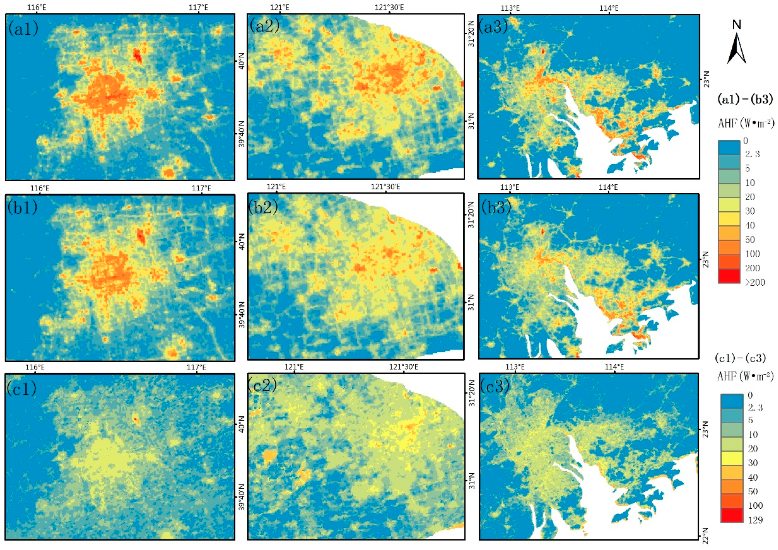
The AHF estimation results of the three indexes in Beijing, Shanghai, and Guangdong are shown in Figure 8. By comparing the spatial morphology of the estimation results, the characteristics and differences of the estimation results of different indexes can be well recognized.
Through the comparison, it is found that the estimation results of the VANUI and NTLnor are relatively consistent on the whole. Moreover, the spatial pattern of AHF in the urban center can be well reflected, and the network distribution of road within the city can be clearly seen from the results, indicating that the results can effectively express the regional characteristics of AHF within the city.
The estimation results of the HSI have obvious saturation phenomenon in the urban center, which cannot reflect the high-value AHF distribution, and have poor performance on the regional characteristics of AHF within the city. It may be that the distribution characteristics and combination mode of factors, such as vegetation cover and human activities in the study area, influence the estimation results of the HSI.
6. Conclusions
The refined AHF mapping in China in the year 2016 is achieved in this study. First of all, the energy-consumption inventory approach is used to estimate the AHE and AHF values of the municipal (state, district, league) administrative regions. Next, the gridded AHF partition estimation models are constructed based on multi-source remote sensing data and the AHF data of the administrative division units. The performance and accuracy of different estimation models constructed based on multiple indexes are analyzed and compared in partitions. The set of optimal model is determined as the AHF partition estimation scheme. Finally, the refined AHF mapping with a resolution of 500 m was realized in China based on the model. The conclusions are as follows:
- The estimated results of AHE and AHF values based on the energy-consumption inventory approach show that the AHE and AHF of provinces in China are quite different. The provinces with high AHE are Shandong, Guangdong, Jiangsu, and Hebei. Among them, the AHE in Shandong province is the highest, accounting for 10.17% of the country’s total AHE. The AHF values are compared in provinces. AHF in Shanghai is the highest, reaching 12.56 W·m−2, which is much higher than other provincial AHF values, followed by Tianjin, Beijing, and Jiangsu. The AHF values are 5.92 W·m−2, 3.35 W·m−2, and 3.10 W·m−2, respectively.
- There are significant correlations between AHF and VANUI, NTLnor. Among them, the fitting R2 value of the VANUI and AHF in sub-regions is between 0.63 and 0.94. The fitting R2 value of NTLnor and AHF is between 0.69 and 0.95, and both of them are applicable to estimating large-scale AHF in China. The distribution characteristics and combination mode of vegetation cover, human activities, and other factors in the study area may have great influence on the estimation results of the HSI. The HSI has obvious regional limitations in the application of large-scale AHF estimation.
- Compared with other AHF products, it is found that the AHF results of this study have higher spatial heterogeneity and can better characterize the spatial distribution pattern of AHF in a region. There are certain advantages to obtain fine AHF data by using the AHF partition estimation scheme, which can better realize AHF estimation according to the characteristics of AH emissions within sub-regions.
The AHF partition estimation scheme proposed in this study realizes the gridded AHF estimation in China. The refined AHF data with a resolution of 500 m obtained in this study can provide a support for the urban heat island and climatic and environmental researches. Since the statistical data are based on the administrative division unit, the model proposed at present cannot achieve the partition study of different AHF components, which still needs further study.
Author Contributions
Conceptualization, D.H.; methodology, S.W. and S.C.; validation, S.W. and C.Y. writing—original draft, S.W.; writing—review and editing, D.H., S.C., C.Y.
Funding
This research was supported by the National Natural Science Foundation of China (Number: 41671339) and National Key Research and Development Program of China (Number: 2017YFB0504102).
Acknowledgments
The authors would like to thank the National Bureau of Statistics and Local Bureau of Statistics of China for providing socio-economic data and energy-consumption data, and the United States Geological Survey and the National Oceanic and Atmospheric Administration for providing remote sensing data. We also want to express our gratitude to the reviewers and editors for their valuable comments and suggestions.
Conflicts of Interest
The authors declare no conflict of interest.
References
- Ichinose, T.; Shimodozono, K.; Hanaki, K. Impact of anthropogenic heat on urban climate in Tokyo. Atmos. Environ. 1999, 33, 3897–3909. [Google Scholar] [CrossRef]
- Fan, H.; Sailor, D. Modeling the impacts of anthropogenic heating on the urban climate of Philadelphia: A comparison of implementations in two PBL schemes. Atmos. Environ. 2005, 39, 73–84. [Google Scholar] [CrossRef]
- Pal, S.; Xueref-Remy, I.; Ammoura, L.; Chazette, P.; Gibert, F.; Royer, P.; Dieudonné, E.; Dupont, J.-C.; Haeffelin, M.; Lac, C.; et al. Spatio-temporal variability of the atmospheric boundary layer depth over the Paris agglomeration: An assessment of the impact of the urban heat island intensity. Atmos. Environ. 2012, 63, 261–275. [Google Scholar] [CrossRef]
- Siân, L.; Janet, B.; Humphrey, L. Case study of an urban heat island in London, UK: Comparison between observations and a high resolution numerical weather prediction model. In Proceedings of the European Meteorological Society Annual Meeting, Reading, UK, 9–13 September 2013. [Google Scholar]
- Young-Hee, R.; Jong-Jin, B.; Sang-Hyun, L. Effects of anthropogenic heat on ozone air quality in a megacity. Atmos. Environ. 2013, 80, 20–30. [Google Scholar]
- Iamarino, M.; Beevers, S.; Grimmond, C.S.B. High-resolution (space, time) anthropogenic heat emissions: London 1970–2025. Int. J. Cimatol. 2012, 32, 1754–1767. [Google Scholar] [CrossRef]
- Lee, S.H.; Song, C.K.; Baik, J.J.; Park, S.U. Estimation of anthropogenic heat emission in the Gyeong-In region of Korea. Theor. Appl. Climatol. 2009, 96, 3–4. [Google Scholar] [CrossRef]
- Smith, C.; Lindley, S.; Levermore, G. Estimating spatial and temporal patterns of urban anthropogenic heat fluxes for UK cities: The case of Manchester. Theor. Appl. Climatol. 2009, 98, 19–35. [Google Scholar] [CrossRef]
- Sailor, D.J. A review of methods for estimating anthropogenic heat and moisture emissions in the urban environment. Int. J. Cimatol. 2010, 31, 189–199. [Google Scholar] [CrossRef]
- Best, M.J.; Grimmond, C.S.B. Investigation of the impact of anthropogenic heat flux within an urban land surface model and PILPS-urban. Theor. Appl. Climatol. 2016, 126, 51–60. [Google Scholar] [CrossRef]
- Park, C.; Schade, G.W.; Werner, N.D.; Sailor, D.J.; Kim, C.H. Comparative estimates of anthropogenic heat emission in relation to surface energy balance of a subtropical urban neighborhood. Atmos. Environ. 2016, 126, 182–191. [Google Scholar] [CrossRef]
- Heiple, S.; Sailor, D.J. Using building energy simulation and geospatial modeling techniques to determine high resolution building sector energy consumption profiles. Energy Build. 2008, 40, 1426–1436. [Google Scholar] [CrossRef]
- Sailor, D.J.; Vasireddy, C. Correcting aggregate energy consumption data to account for variability in local weather. Environ. Model. Softw. 2006, 21, 733–738. [Google Scholar] [CrossRef]
- Dong, Y.; Varquez, A.C.G.; Kanda, M. Global anthropogenic heat flux database with high spatial resolution. Atmos. Environ. 2017, 150, 276–294. [Google Scholar] [CrossRef]
- Sun, R.H.; Wang, Y.N.; Chen, L.D. A distributed model for quantifying temporal-spatial patterns of anthropogenic heat based on energy consumption. J. Clean. Prod. 2018, 170, 601–609. [Google Scholar] [CrossRef]
- Grimmond, C.S.B. The suburban energy balance: Methodological considerations and results for a Mid-latitude west coast city under winter and spring conditions. Int. J. Cimatol. 2010, 12, 481–497. [Google Scholar] [CrossRef]
- Ferreira, M.J.; Oliveira, A.P.D.; Soares, J. Anthropogenic heat in the city of São Paulo, Brazil. Theor. Appl. Climatol. 2011, 104, 43–56. [Google Scholar] [CrossRef]
- Quah, A.K.L.; Roth, M. Diurnal and weekly variation of anthropogenic heat emissions in a tropical city, Singapore. Atmos. Environ. 2012, 46, 92–103. [Google Scholar] [CrossRef]
- Sailor, D.J.; Georgescu, M.; Milne, J.M. Development of a national anthropogenic heating database with an extrapolation for international cities. Atmos. Environ. 2015, 118, 7–18. [Google Scholar] [CrossRef] [Green Version]
- Sutton, P.; Roberts, D.; Elvidge, C.; Baugh, K. Census from heaven: An estimate of the global human population using night-time satellite imagery. Int. J. Remote Sens. 2001, 22, 3061–3076. [Google Scholar] [CrossRef]
- Doll, C.N.H.; Muller, J.-P.; Morley, J.G. Mapping regional economic activity from night-time light satellite imagery. Ecol. Econ. 2006, 57, 75–92. [Google Scholar] [CrossRef]
- Yue, W.; Gao, J.; Yang, X. Estimation of Gross Domestic Product Using Multi-Sensor Remote Sensing Data: A Case Study in Zhejiang Province, East China. Remote Sens. 2014, 6, 7260–7275. [Google Scholar] [CrossRef] [Green Version]
- Chen, Y.; Jiang, W.M.; Zhang, N.; He, X.F.; Zhou, R.W. Numerical simulation of the anthropogenic heat effect on urban boundary layer structure. Theor. Appl. Climatol. 2009, 97, 123–134. [Google Scholar] [CrossRef]
- Li, X.; Xu, H.; Chen, X.; Li, C. Potential of NPP-VIIRS nighttime Light imagery for modeling the regional economy of China. Remote Sens. 2013, 5, 3057–3081. [Google Scholar] [CrossRef]
- Coscieme, L.; Pulselli, F.M.; Bastianoni, S.; Elvidge, C.D.; Anderson, S.; Sutton, P.C. A thermodynamic geography: Night-time satellite imagery as a proxy measure of emergy. Ambio 2014, 43, 969–979. [Google Scholar] [CrossRef]
- Zhou, Y.; Ma, T.; Zhou, C.; Xu, T. Nighttime light derived assessment of regional inequality of socioeconomic development in China. Remote Sens. 2015, 7, 1242–1262. [Google Scholar] [CrossRef]
- Yang, W.; Chen, B.; Cui, X. High-resolution mapping of anthropogenic heat in China from 1992 to 2010. Int. J. Environ. Res. Public Health 2014, 11, 4066–4077. [Google Scholar] [CrossRef]
- Lu, D.; Tian, H.; Zhou, G.; Ge, H. Regional mapping of human settlements in southeastern China with multi-sensor remotely sensed data. Remote Sens. Environ. 2008, 112, 3668–3679. [Google Scholar] [CrossRef]
- Ma, P.; Wu, J.; Yang, X.; Qi, J. Spatialization of anthropogenic heat emission based on multi-source remote sensing information-a case study of Zhejiang province. China Environ. Sci. 2016, 36, 314–320. [Google Scholar]
- Chen, S.; Hu, D. Parameterizing Anthropogenic Heat Flux with an Energy-Consumption Inventory and Multi-Source Remote Sensing Data. Remote Sens. 2017, 9, 1165. [Google Scholar] [CrossRef]
- Weng, Q.; Lu, D.; Schubring, J. Estimation of land surface temperature–vegetation abundance relationship for urban heat island studies. Remote Sens. Environ. 2004, 89, 467–483. [Google Scholar] [CrossRef]
- Zhang, Q.; Schaaf, C.; Seto, K.C. The Vegetation Adjusted NTL Urban Index: A new approach to reduce saturation and increase variation in nighttime luminosity. Remote Sens. Environ. 2013, 129, 32–41. [Google Scholar] [CrossRef]
- Chen, S.; Hu, D.; Wong, M.S.; Ren, H.; Cao, S.; Yu, C.; Ho, H.C. Characterizing spatiotemporal dynamics of anthropogenic heat fluxes: A 20-year case study in Beijing–Tianjin–Hebei region in China. Environ Pollut. 2019, 249, 923–931. [Google Scholar] [CrossRef]
- National Bureau of Statistics of China: Chinese Statistical Yearbook. Available online: http://www.stats.gov.cn/tjsj/ndsj/ (accessed on 14 February 2019).
- The Level-1 and Atmosphere Archive and Distribution System (LAADS) Distributed Active Archive Center (DAAC). Available online: https://ladsweb.nascom.nasa.gov/search/ (accessed on 14 February 2019).
- National Oceanic and Atmospheric Administration/National Geophysical Data Center (NOAA/NGDC). Available online: https://ngdc.noaa.gov/og/viirs/download_dnb_composites.html (accessed on 14 February 2019).
- Zeng, C.; Ling, X.; Wang, K.; Liu, K.; Wang, T. Spatial pattern and input-output analysis of industrial competitiveness in China’s eight economic zones. Prog Geog. 2012, 31, 1005–1012. [Google Scholar]
- Rosenzweig, C. Climate Change and Cities: First Assessment Report of the Urban Climate Change Research Network; Cambridge University Press: New York, NY, USA, 2011; Volume 33, pp. 242–244. [Google Scholar]
- Chen, B.; Shi, G.; Dai, T.; Shen, Y.; Wang, B.; Yang, S.; Zhao, J. Climate forcing due to anthropogenic heat release over China. Clim. Environ. Res. 2011, 16, 717–722. [Google Scholar]
- Xie, M.; Zhuang, K.; Wang, T.; Feng, W.; Zhuang, X.; Chen, F.; OuYang, Y.; Liu, Z.J. Study on the distribution characteristics of anthropogenic heat in China. China Environ. Sci. 2015, 35, 728–734. [Google Scholar]
- Allen, L.; Lindberg, F.; Grimmond, C.S.B. Global to city scale urban anthropogenic heat flux: Model and variability. Int. J. Climatol. 2011, 31, 1990–2005. [Google Scholar] [CrossRef]
- Lindberg, F.; Grimmond, C.S.B.; Nithiandamdan, Y.; Kotthaus, S.; Allen, L. Impact of city changes and weather on anthropogenic heat flux in Europe 1995–2015. Urban Clim. 2013, 4, 1–15. [Google Scholar] [CrossRef]
- Flanner, M.G. Integrating anthropogenic heat flux with global climate models. Geophys. Res. Lett. 2009, 36, 270–271. [Google Scholar] [CrossRef]
- Socioeconomic Data and Applications Center (SEDAC). Available online: http://sedac.ciesin.columbia.edu/data/collection/gpw-v4/ (accessed on 2 April 2019).
- Center for International Earth Science Information Network (CIESIN), Columbia University. Documentation for the Gridded Population of the World, Version 4 (GPWv4), Revision 11 Data Sets; NASA Socioeconomic Data and Applications Center (SEDAC): Palisades, NY, USA, 2018. [CrossRef]
- Ting, M.; Chenghu, Z.; Tao, P.; Susan, H.; Junfu, F. Quantitative estimation of urbanization dynamics using time series of DMSP/OLS nighttime light data: A comparative case study from China’s cities. Remote Sens. Environ. 2012, 124, 99–107. [Google Scholar]
- Elvidge, C.D.; Baugh, K.E.; Kihn, E.A.; Kroehl, H.W.; Davis, E.R.; Davis, C.W. Relation between satellite observed visible-near infrared emissions, population, economic activity and electric power consumption. Int. J. Remote Sens. 1997, 18, 1373–1379. [Google Scholar] [CrossRef]
- Jing, X.; Shao, X.; Cao, C.; Fu, X.; Yan, L. Comparison between the Suomi-NPP day-night band and DMSP-OLS for correlating Socio-Economic variables at the provincial level in China. Remote Sens. 2016, 8, 17. [Google Scholar] [CrossRef]
Figure 1.
Study area division. northern coastal region (NCR); eastern coastal region (ECR); southern coastal region (SCR); middle Yangtze River region (MYAR); southwest region (SWR); northeast region (NER); middle Yellow River region (MYER); northwest region (NWR).
Figure 1.
Study area division. northern coastal region (NCR); eastern coastal region (ECR); southern coastal region (SCR); middle Yangtze River region (MYAR); southwest region (SWR); northeast region (NER); middle Yellow River region (MYER); northwest region (NWR).

Figure 2.
Flowchart of the gridded anthropogenic heat flux (AHF) estimation scheme.

Figure 3.
The anthropogenic heat emission (AHE) and AHF results in 2016. (a) AHE of different heat sources in provinces. (b) AHF of the provinces.
Figure 3.
The anthropogenic heat emission (AHE) and AHF results in 2016. (a) AHE of different heat sources in provinces. (b) AHF of the provinces.

Figure 4.
Linear regression relationship between AHF and vegetation adjusted nighttime light urban index (VANUI or NTLnor) in sub-regions. (a) ECR; (b) MYER; (c) MYAR; (d) SCR; (e) SWR; (f) NER; (g) NCR; (h) NWR.
Figure 4.
Linear regression relationship between AHF and vegetation adjusted nighttime light urban index (VANUI or NTLnor) in sub-regions. (a) ECR; (b) MYER; (c) MYAR; (d) SCR; (e) SWR; (f) NER; (g) NCR; (h) NWR.

Figure 5.
The AHF estimation results in China in the year 2016. (a) Beijing–Tianjin–Hebei region; (b) Yangtze River delta region; (c) Pearl River delta region.
Figure 5.
The AHF estimation results in China in the year 2016. (a) Beijing–Tianjin–Hebei region; (b) Yangtze River delta region; (c) Pearl River delta region.

Figure 6.
The AHF estimation results and high-value area distribution validation of cities. (a) Beijing; (b) Shanghai; (c) Guangzhou; (d–f) high-resolution images of corresponding cities. Note: (a,d): 1. Beijing capital international airport; 2. Beijing railway station; 3. Beijing south railway station;4. Beijing Nanyuan airport; 5. Beijing west railway station; 6. Beijing east railway station; (b,e): 1. Shanghai Pudong international airport; 2. Shanghai Hongqiao airport; 3. Shanghai south railway station; 4. Shanghai Gaodong helipad; 5.Oriental Pearl Tower; 6. Songjiang south station; 7. Shanghai Disney; (c,f): 1. Guangzhou Baiyun airport; 2. Guangzhou east railway station; 3. Guangzhou station; 4. Tangxi railway station; 5. Canton Tower; 6. Industry zone.

Figure 7.
The comparison of the AHF results of the three models (a) The results of this study resampled to 1 km resolution. (b) The results of the large scale urban consumption of the energy (LUCY) model. (c) The results of this study resampled to 2.5 arc-min resolution. (d) The results of Flanner et al.

Figure 8.
The AHF estimation results of the three indexes. (a1–a3) VANUI; (b1–b3) normalized nighttime light data (NTLnor); (c1–c3) HSI.
Figure 8.
The AHF estimation results of the three indexes. (a1–a3) VANUI; (b1–b3) normalized nighttime light data (NTLnor); (c1–c3) HSI.


Table 1.
The AHF partition estimation model and its goodness of fit.
| Sub-Regions | AHF Estimation Model | Goodness of Fit |
|---|---|---|
| ECR | AHF = 222.42 × NTLnor + 0.59 | 0.95 |
| SWR | AHF = 245.19 × NTLnor + 0.22 | 0.80 |
| NCR | AHF = 303.22 × NTLnor + 1.29 | 0.69 |
| NWR | AHF = 637.93 × NTLnor − 0.15 | 0.73 |
| MYER | AHF = 997.68 × VANUI + 0.36 | 0.83 |
| SCR | AHF = 1304.90 × VANUI − 0.20 | 0.82 |
| MYAR | AHF =439.55 × VANUI + 0.45 | 0.80 |
| NER | AHF = 546.42 × VANUI + 0.13 | 0.75 |
Table 2.
Comparison of AHF estimation results in this study with the existing AHF results.
| The Sample Position | AHF (W·m−2) | ||
|---|---|---|---|
| Chen (2008) | Xie (2010) | This Study (2016) | |
| Beijing | 4.00 | 3.71 | 5.84 |
| Tianjin | 5.10 | 4.47 | 6.91 |
| Shanghai | 16.54 | 14.46 | 12.53 |
| Jiangsu | 2.32 | 2.61 | 2.81 |
| Zhejiang | 1.60 | 1.63 | 1.92 |
| Guangdong | 1.40 | 1.82 | 4.53 |
| Shandong | 2.16 | 2.31 | 2.99 |
Table 3.
AHF contribution rates of different grades in sub-regions.
| AHF Grades (W·m−2) | Contribution Rate (%) | ||
|---|---|---|---|
| NCR | SCR | ECR | |
| 0–10 | 51.79 | 24.21 | 37.39 |
| 10–20 | 15.36 | 22.68 | 25.33 |
| 20–30 | 11.01 | 17.40 | 19.43 |
| 30–40 | 8.05 | 12.51 | 11.64 |
| 40–50 | 5.76 | 7.95 | 4.01 |
| 50–60 | 3.34 | 5.14 | 1.09 |
| 60–70 | 1.92 | 3.12 | 0.47 |
| 70–80 | 1.13 | 2.01 | 0.17 |
| 80–90 | 0.47 | 1.47 | 0.14 |
| 90–00 | 0.28 | 0.99 | 0.04 |
| >100 | 0.89 | 2.52 | 0.29 |
Table 4.
Goodness of fit between indexes and AHF.
| Sub-Regions | Goodness of Fit (R2) | ||
|---|---|---|---|
| AHF–VANUI | AHF–NTLnor | AHF–HSI | |
| ECR | 0.94 | 0.95 | 0.83 |
| MYER | 0.83 | 0.82 | 0.01 |
| MYAR | 0.80 | 0.77 | 0.56 |
| NER | 0.75 | 0.70 | 0.09 |
| SWR | 0.74 | 0.80 | 0.20 |
| SCR | 0.82 | 0.80 | 0.52 |
| NCR | 0.66 | 0.69 | 0.34 |
| NWR | 0.63 | 0.73 | 0.05 |
© 2019 by the authors. Licensee MDPI, Basel, Switzerland. This article is an open access article distributed under the terms and conditions of the Creative Commons Attribution (CC BY) license (http://creativecommons.org/licenses/by/4.0/).
Share and Cite
MDPI and ACS Style
Wang, S.; Hu, D.; Chen, S.; Yu, C. A Partition Modeling for Anthropogenic Heat Flux Mapping in China. Remote Sens. 2019, 11, 1132. https://0-doi-org.brum.beds.ac.uk/10.3390/rs11091132
AMA Style
Wang S, Hu D, Chen S, Yu C. A Partition Modeling for Anthropogenic Heat Flux Mapping in China. Remote Sensing. 2019; 11(9):1132. https://0-doi-org.brum.beds.ac.uk/10.3390/rs11091132
Chicago/Turabian StyleWang, Shasha, Deyong Hu, Shanshan Chen, and Chen Yu. 2019. "A Partition Modeling for Anthropogenic Heat Flux Mapping in China" Remote Sensing 11, no. 9: 1132. https://0-doi-org.brum.beds.ac.uk/10.3390/rs11091132
Note that from the first issue of 2016, this journal uses article numbers instead of page numbers. See further details here.