Hyperspectral Image Super-Resolution by Deep Spatial-Spectral Exploitation

1
School of Computer Science and Technology, Xi’an University of Technology, Xi’an 710048, China
2
School of Telecommunications Engineering, Xi’dian University, Xi’an 710071, China
*
Author to whom correspondence should be addressed.
Remote Sens. 2019, 11(10), 1229; https://0-doi-org.brum.beds.ac.uk/10.3390/rs11101229
Submission received: 11 April 2019
/
Revised: 9 May 2019
/
Accepted: 16 May 2019
/
Published: 23 May 2019
(This article belongs to the Special Issue Image Processing and Spatial Neighbourhoods for Remote Sensing Data Analysis)
Abstract
:Limited by the existing imagery sensors, hyperspectral images are characterized by high spectral resolution but low spatial resolution. The super-resolution (SR) technique aiming at enhancing the spatial resolution of the input image is a hot topic in computer vision. In this paper, we present a hyperspectral image (HSI) SR method based on a deep information distillation network (IDN) and an intra-fusion operation. Specifically, bands are firstly selected by a certain distance and super-resolved by an IDN. The IDN employs distillation blocks to gradually extract abundant and efficient features for reconstructing the selected bands. Second, the unselected bands are obtained via spectral correlation, yielding a coarse high-resolution (HR) HSI. Finally, the spectral-interpolated coarse HR HSI is intra-fused with the input HSI to achieve a finer HR HSI, making further use of the spatial-spectral information these unselected bands convey. Different from most existing fusion-based HSI SR methods, the proposed intra-fusion operation does not require any auxiliary co-registered image as the input, which makes this method more practical. Moreover, contrary to most single-based HSI SR methods whose performance decreases significantly as the image quality gets worse, the proposal deeply utilizes the spatial-spectral information and the mapping knowledge provided by the IDN, which achieves more robust performance. Experimental data and comparative analysis have demonstrated the effectiveness of this method.

1. Introduction
Hyperspectral imagery sensors usually collect reflectance information of objects in hundreds of contiguous bands over a certain electromagnetic spectrum [1], and the hyperspectral image (HSI) can simultaneously obtain a set of two-dimensional images (or bands) [2]. These rich bands play an important role in discriminating different objects by their spectral signatures [3], and making them widely applicable in classification [4] and anomaly detection [5]. However, limited by the existing imaging sensor technologies, HSIs are characterized by low spatial resolution, which results in limitation of their applications’ performance. As a type of signal post-processing technique, HSI super-resolution (SR) can improve the spatial resolution of the HSI without modifying the imagery hardware, which is a hot issue in computer vision.
HSI SR has been studied for a long time in remote sensing and many methods have been proposed to improve the spatial resolution of the HSIs. According to the number of input images, these methods can be roughly classified into two types: the fusion-based HSI SR methods and the single-based ones.
The fusion-based approaches are based on the assumption that multiple fully-registered observations of the same scene are accessible. Dong et al. [6] proposed a nonnegative structured sparse representation approach, which jointly estimates the dictionary and sparse code of the high-resolution(HR) HSI based on the input low-resolution (LR) HSI and HR panchromatic (PAN) image. By utilizing the similarities between pixels in the super-pixel, Fang et al. [7] proposed a super-pixel based sparse representation method. Dian et al. [8] presented a non-local sparse tensor factorization HSI SR method, which achieves a fuller exploitation of the spatial-spectral structures in the HSI. For matrixing three-dimensional HSI and multispectral image (MSI) that are prone to inducing loss of structural information, Kanatsoulis et al. [9] addressed the problem from a tensor perspective and established a coupled tensor factorization framework. Zhang et al. [10] discovered that the clustering manifold structure of the latent HSI can be well preserved in the spatial domain of the input conventional image, and proposed to super-resolve the HSI by this discovery. Considering that the sparse based methods tackle each pixel independently, Han et al. [11] utilized a self-similarity prior as the constraint for sparse representation of the HSI and MSI. With the auxiliary HR image being another input of this kind of methods, more information is obtained, and this type of methods often achieves a better spatial enhancement. However, in reality, the auxiliary fully-registered HR description of the same scene is always hard or impossible to be achieved, which restricts the practicability of this type of methods.
The single-based HSI SR methods can be further divided into the sub-pixel mapping ones and the direct single-based ones. Sub-pixel mapping methods aim at estimating the fractional abundance of pure ground objects within a mixed pixel, and obtain the probabilities of sub-pixels to belong to different land cover classes [12]. Irmak [13] firstly utilized the virtual dimensionality to determine the number of endmembers in the scene and computed the abundance maps. The corresponding HR abundance maps are firstly obtained by maximum a posteriori method. Then, they are utilized to reconstruct the HR HSI. This kind of methods tackles the SR problem from the endmember extraction and fractional abundance estimation. However, the noise generated by the unmixing operation is inevitable during the mapping operation, which makes a negative influence on the SR process. Additionally, sub-pixel mapping methods are usually applied to certain applications, such as classification and target detection, for overcoming the limitation in spatial resolution. Arun et al. [14] explored convolutional neural network to jointly optimize the unmixing and mapping operation in a supervised manner. Xu et al. [15] presented a joint spectral-spatial mapping model to obtain the probabilities of sub-pixels to belong to different land cover classes, and obtained a resolution-enhanced image.
The direct single-based HSI SR methods aim at reconstructing an HR HSI with only one LR HSI. Inspired by the achievements in deep learning based RGB image SR methods, Yuan et al. [16] and He et al. [17] proposed to super-resolve each band individually by transfer learning. Considering the three-dimensional data characteristics of HSIs, Mei et al. [18] proposed a 3D-CNN to exploit both the spatial context and the spectral correlation. However, as there are usually hundreds of bands in the HSI, super-resolving the bands individually consumes much complexity. Moreover, as the image quality decreases, super-resolving each single band will be much more difficult, which will induce severe performance degradation.
In this paper, we propose an HSI SR method by combining an information distillation network (IDN) [19] with an intra-fusion operation to make a deep exploitation of the spatial-spectral information. During the implementation process, bands are firstly selected by certain interval, and then super-resolved by taking advantage of their spatial information and the spatial mapping learnt by the IDN model. The IDN was trained by 91 images from Yang et al. [20] and 200 images from the Berkeley Segmentation dataset [21]. Three data augmentation ways were applied to make full use of the training data and 2619 images were obtained. The IDN was designed to learn the spatial mapping between Y channels of the low-resolution RGB images and those of the corresponding high-resolution RGB images. Each single band in HSI can also be tackled as its Y channel at current wavelength. In this way, it is reasonable to transfer the IDN for the HSI SR. Secondly, spectral correlation is utilized to achieve a complete but coarse HR HSI. In addition, the information these unselected bands convey is further exploited by intra-fusing with the coarse HR HSI, resulting a finer HR HSI. In this way, both spatial and spectral information of the input LR HSI is fully-utilized, which contributes to the robust and acceptable performance.The main contributions of this work are summarized as follows:
1. We adopt a scalable SR strategy for super-resolving the HSI. Firstly, an IDN is used for super-resolving the interval-selected bands individually, a process exploiting their spatial information and the mapping learned by the IDN. Secondly, the unselected bands are fast interpolated via cubic Hermit spline method, which uses the high spectral correlation in the HSI to obtain a coarse HR HSI. Both spatial and spectral information is utilized. Meanwhile, contrary to super-resolving the HSI band by band via some certain methods, this scalable SR strategy achieves a tradeoff between high quality and high efficiency.
2. Most existing single-based methods super-resolve bands in the HSI individually, which neglects the spectral information. In this way, their performance is highly correlated to the images’ spatial quality. The proposed method deeply utilizes both the spatial and spectral information in the HSI, and its performance is more robust.
3. To deeply use the information the input LR HSI conveys, intra-fusion is made between the spectral-interpolated coarse HR HSI and the input LR HSI. Different from most fusion methods, which require another co-registered image as the input, the other input of the proposed intra-fusion is an intermediate outcome of the SR processing, which fully exploits the information the LR HSI conveys in a subtle way.
2. Proposed Method
In this section, we present the four main parts of the proposed method: framework overview, bands’ selection and super-resolution by IDN, unselected bands’ super-resolution, and intra-fusion. Detailed descriptions of these four parts are presented in the following subsections.
2.1. Framework Overview
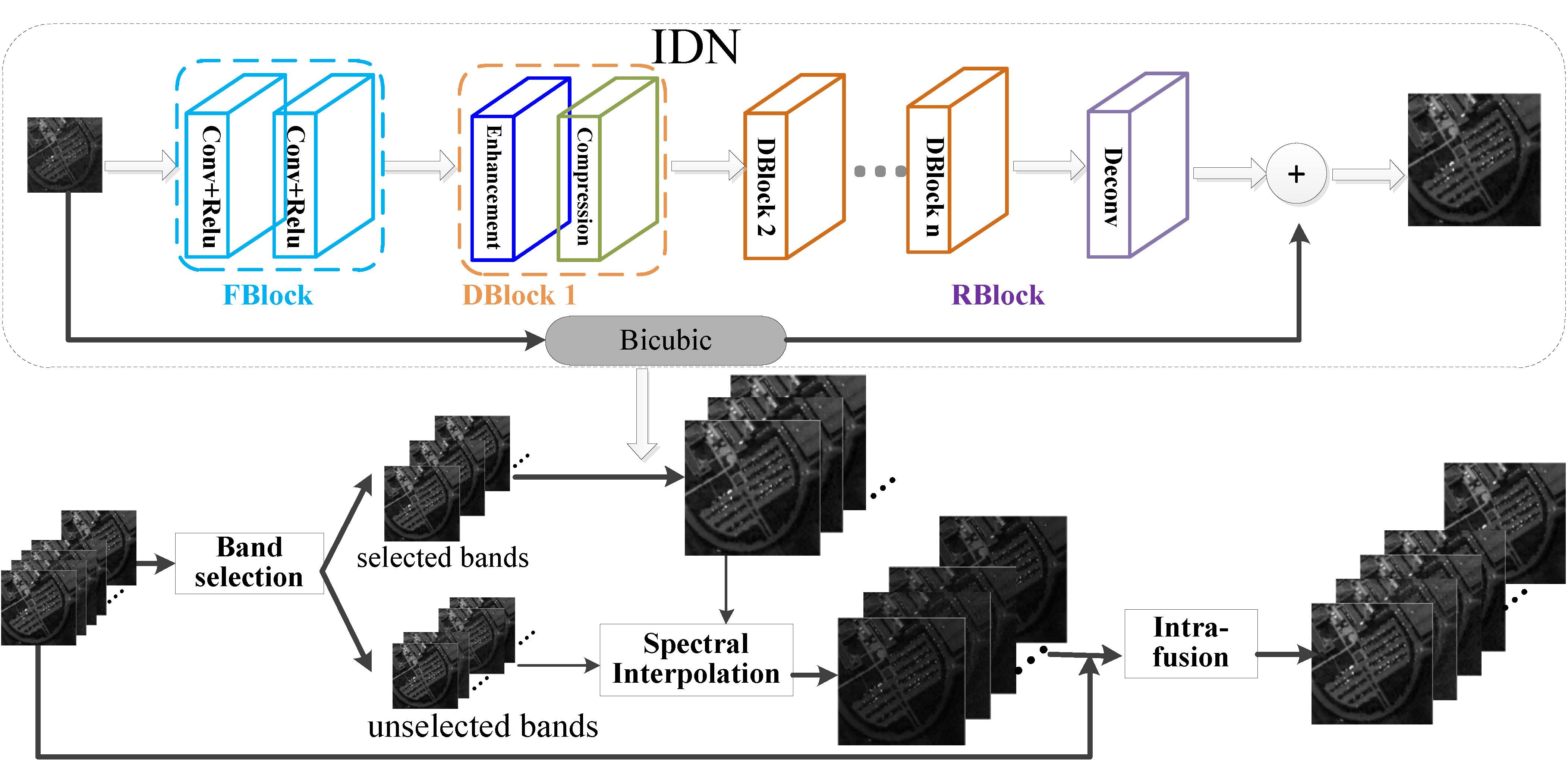
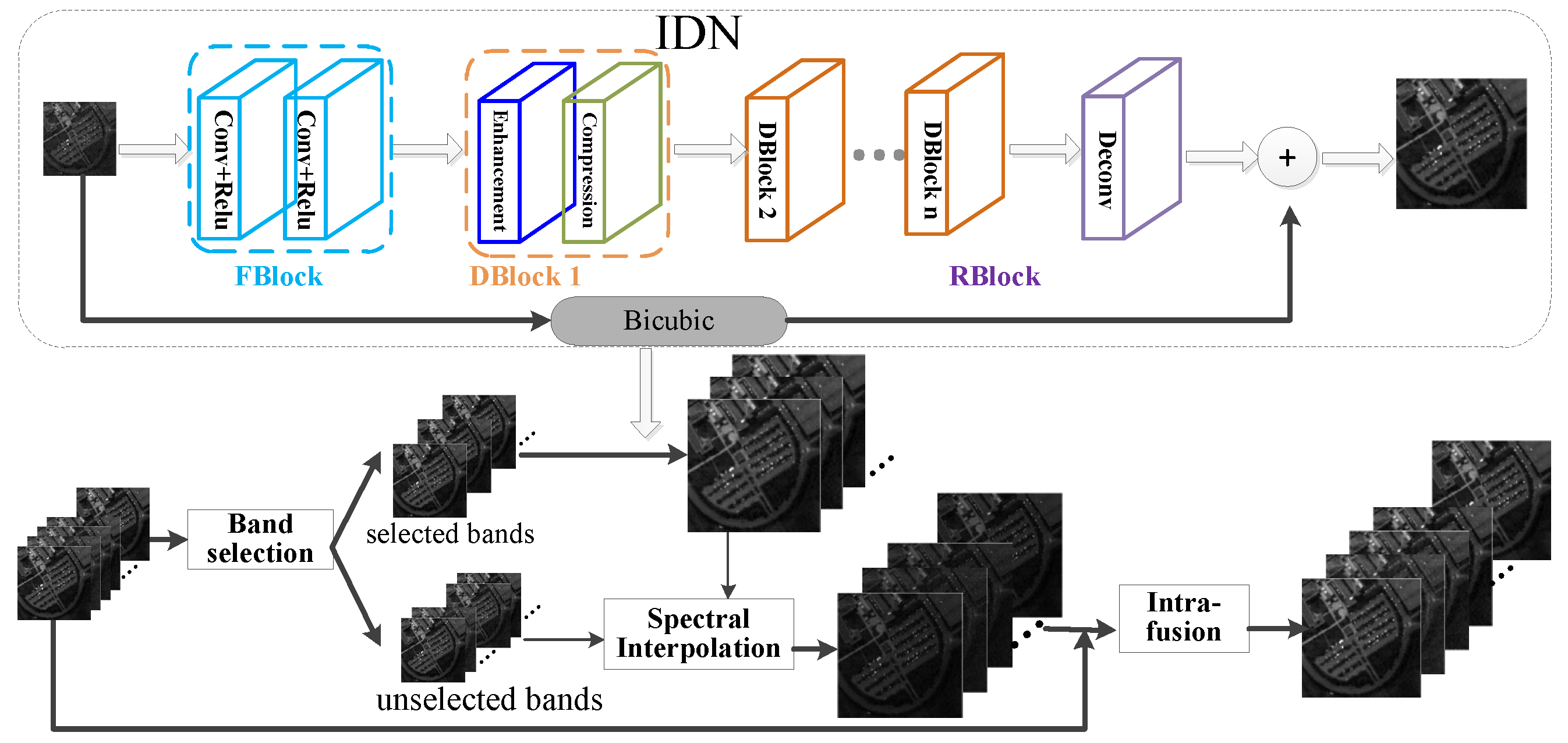
Figure 1 illustrates the workflow of the proposed HSI SR method. The input data are one LR HSI. Bands are first selected by a certain distance and super-resolved via IDN with respect to their spatial information. Then, unselected bands are super-resolved by utilizing their spectral correlation to obtain a coarse but integrated HR HSI. Furthermore, this coarse HR HSI is intra-fused with the input LR HSI to further use the information these unselected bands convey.
To facilitate discussion, we clarify the notations of some frequently used terms. The input LR HSI and the desired HR HSI are represented as and , where w and h denote the width and height of the input LR HSI. s and n denote the scaling factor and the number of bands, respectively. and denote the coarse HR HSI and the intra-fused fine HR HSI, respectively.
2.2. Bands’ Selection and Super-Resolution by IDN
This part firstly analyzes the correlation between the bands in the HSI and depicts the rationality of interval setting, and then super-resolves the selected bands via IDN.
2.2.1. Correlation Analysis
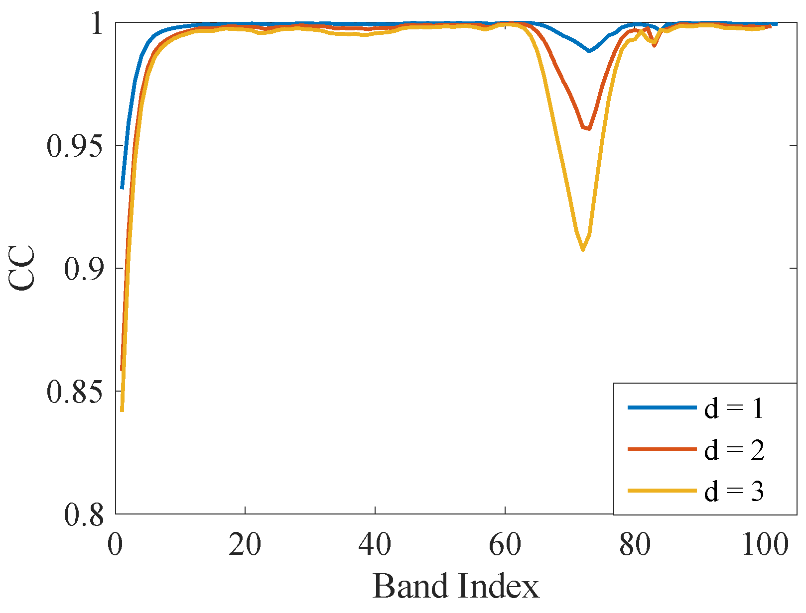
For HSIs, their neighboring bands are highly correlated in the spectral domain [22]. Figure 2 plots the correlation coefficient curves of the Pavia university scene HSI, a remote-sensing HSI widely applied in classification [23].
The value on the x-axis is the index of the current band . The legend denotes the interval between and the other neighboring band . The value on the y-axis is the correlation coefficient between and . According to the three curves in Figure 2, although correlation decreases as the band gets further from the current one, most bands are highly correlated to their neighboring bands, whose correlation coefficients are larger than 0.95. Moreover, as the image quality decreases, most high-frequency in the images are damaged, the correlation coefficient between neighboring bands is supposed to be higher (related experiments have been described in Section 3). Hence, to achieve a high efficiency without performance loss, it is rational and necessary to firstly select some bands by certain distance and super-resolve the selected bands by utilizing their spatial information. Contrary to super-resolving each bands in the HSI, this operation will highly reduce the computational complexity with negligible performance degradation.
2.2.2. Super-Resolution via IDN
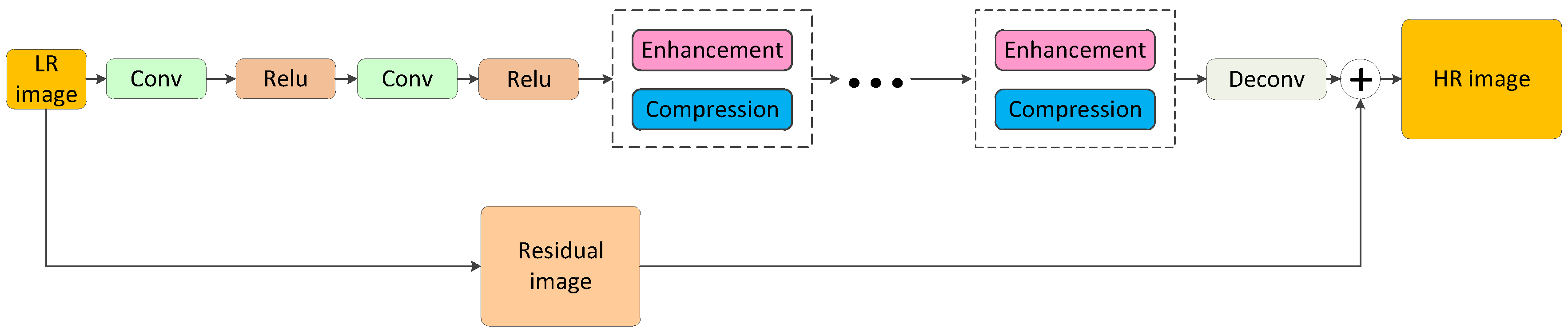
Figure 3 has shown the general architecture of the IDN, a process consisting of three parts, i.e., a feature extraction block, multiple stacked information distillation blocks and a reconstruction block.
The feature extraction block applies two convolution layers to extract the feature maps from the original LR images. The extracted features maps act as the input of the information distillation blocks. Several information distillation blocks are composed by using chained mode, in which each block contains an enhancement unit and a compression unit with stacked style. Finally, a transposed convolution layer without activation function acts as the reconstruction block to obtain the HR image. Compared with the other networks, the IDN extracts feature maps directly from the LR images and utilizes multiple DBlocks to generate the residual representations in HR space. The enhancement unit in each DBlock gathers as much information as possible, and the remaining compression unit distills more useful information, which achieves competitive results with a concise structure.
It should be noted that the network considered two loss functions during the training process. The first one is the widely used mean square error (MSE):
in which N, , and represent the number of training samples, the ith input image patch and the label of the ith input image patch, respectively. Meanwhile, mean absolute error (MAE) is also applied to train the IDN model. The MAE is formulated as:
Specifically, the IDN is first trained with , and then fine-tuned by the .
Having the trained IDN, the spatial resolution of the selected bands in the LR HSI can be enhanced in a fast and efficient way, and the IDN super-resolved HR bands can be denoted as
where the unselected bands are temporarily missing.
2.3. Spectral-Interpolation for the Unselected Bands
Given the super-resolved interval-selected bands, the proposal applies a cubic Hermite spline method to achieve a continuous and smooth entire HR HSI. Cubic Hermite splines are typically used for interpolation of numeric data specified at given argument values, to obtain a smooth continuous function. Compared with the linearity, it can better hold and analyze the mean of the the dependent variables and capture the nature of their relationships [24].
Suppose that the following nodes in the cubic Hermite spline function and their values are given:
in which n denotes the number of the given nodes minus 1, thus it starts from 0. The proposed cubic Hermite spline function describes the mapping between x and y, and is a partition- defined formula.
With these IDN-super-resolved HR bands acting as the given nodes, the cubic Hermite spline function can be applied to obtain one coarse but integrated HR HSI, which can be denoted as:
2.4. Intra-Fusion
According to the above descriptions, the HR HSI is reconstructed by utilizing the spatial information of the selected bands, the mapping learned by the IDN model and the spectral correlation. The information these unselected bands convey is directly neglected. If further utilization of these information is made, it is supposed that a spatial enhancement will be gained. In this way, we propose to get an HR HSI through intra-fusing the spectral-interpolated with the input LR HSI L via the non-negative matrix factorization (NMF) method. Different from most existing fusion methods, the input of the proposed fusion is an intermediate output of the super-resolution process, which is why it is named as intra-fusion. This intra-fusion is more flexible and more practical.
Because of the coarse spatial resolution, pixels in the HSI are usually mixed by different materials. Spectral curves of the HSI usually are mixtures of different pure materials’ reflectance, and these pure materials are called endmembers. Considering the mathematics simplicity and physical effectiveness, each spectral curve can be modeled by a linear mixture model. Let matrix represent the desired HR HSI by concatenating the pixels of HSI H: . The same operation is implemented on the spectral-interpolated HR HSI and the input LR HSI to obtain the and . In this way, the desired HR HSI can be denoted as
where is the endmember matrix, and is the abundance matrix. N denotes the residual. D is the number of endmembers and each column in W represents the spectrum of an endmember. Here, D is obtained by the Neyman–Pearson lemma [25]. Given an HSI with n bands, eigenvalues of its correlation matrix and covariance matrix are computed and sorted as and , respectively. According to the binary hypothesis testing, assume H0: , H1: . According to the preset false alarm rate, a threshold can be computed to maximize the detection rate. In this way, when is greater than , a signal signature is considered to exist. The number of endmembers is obtained by counting the number of eigenvalues that satisfy . In the proposal, the given false alarm rate is set as . Meanwhile, all elements in the matrix W and C are nonnegative.
The spectral-interpolated HR HSI and the input LR HSI can be denoted as:
in which Q is the spectral transform matrix, and is the spatial spread transform matrix. and are the residual matrices. When substituting Equation (6) into Equations (7) and (8), and can be reformulated as
where and denote the spatial degraded abundance matrix and the spectrally degraded matrix, respectively.
During the HSI unmixing procedure, it is expected that the HSI reconstructed by the endmember and coefficient matrices should be close to input image. In this way, the cost functions about the input LR HSI and spectral-interpolated are formulated as and , respectively. NMF was developed to decompose a nonnegative matrix into a product of nonnegative matrices [26]. When applied to the , the cost function is formulated as
During the solving process, both and C are firstly initialized as nonnegative matrices. If is smaller than the desired matrix , a variable k whose value is larger than 1 will be multiplied by to make it next to the . On the other hand, if is larger than , k should be larger than 0 but smaller than 1 to make sure all the elements in are nonnegative. In this way, k is defined as
where denotes the transposition of the matrix. “./” denotes the element-wise division. According to Equation (7), it is noted that the relation between k and constant 1 changes with that between and . Hence, can be updated by the following expression:
The same update strategy is operated on C, W and .
When W and C are obtained, the HR HSI intra-fused by and L is also achieved, which contains both the conveyed spatial information L and the IDN learned spatial mapping correlation. Moreover, this fusion operation does not require any auxiliary HR image as the input, which is more practical. The complete algorithm is summarized in Algorithm 1.
| Algorithm 1: Pseudocode of the proposal. |
 |
3. Experimental Setup and Data Analysis
3.1. Experimental Setup
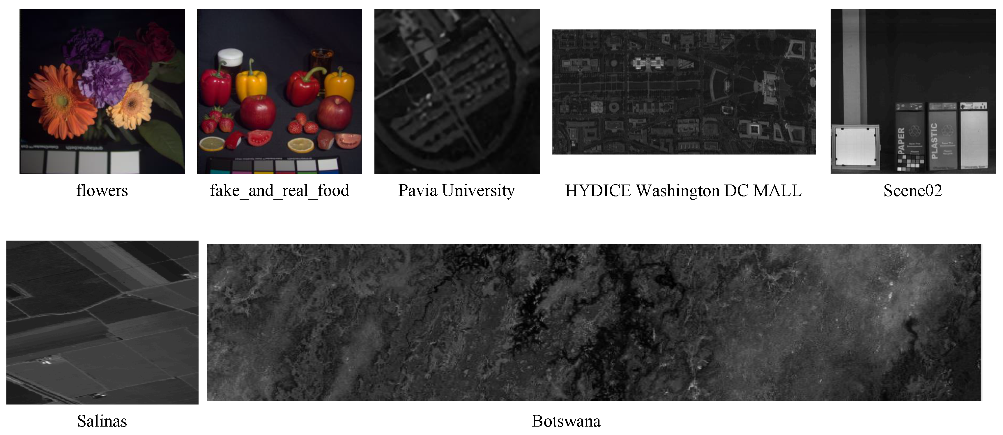
The performance of this proposed method was mainly evaluated on outdoor HSIs obtained via airborne, spaceborne and the ground-based platforms. The outdoor HSIs utilized in the experiments are the Pavia University, Washington DC Mall, Salinas, Botswana and Scene02 datasets. They were acquired by the Reflective Optics Imaging Spectrometer (ROSIS), the Hyperspectral Digital Image Collection Experiment (HYDICE), the Airborne Visible/Infrared Imaging Spectrometer (AVIRIS), the Hyperion sensor on the NASA EO-1 satellite and the Spectral Imagery (SPECIM) hyperspectral camera, respectively. The geometric resolution of the ROSIS and HYDICE are 1.3 m and 1 m, respectively. There are pixels in the original Pavia University, but we selected a region with rich detail to validate the performance. The Washington DC Mall acquisition measured the pixel response from 400 nm to 2400 nm region. Bands in the 900 nm and 1400 nm region where the atmosphere is opaque were omitted from the dataset, leaving 191 bands. The Salinas dataset was collected by the 224-band AVIRIS sensor and 20 water absorption bands were abandoned. The Botswana dataset was acquired at 30 m pixel resolution over a 7.7 km strip in 242 bands covering the 400–2500 nm portion of the spectrum in 10 nm windows. The scene02 HSI consists of pixels and 396 spectral reflectance bands in the wavelength range from 378 nm to 1003 nm. It is noted that these outdoor HSIs cover three different types of surface. Both the Pavia University and Washington DC Mall datasets refer to the building typologies, the Salinas and Botswana datasets refer to the land cover typologies, and the scene02 dataset refers to the man-made material typologies.
Moreover, to validate the proposal’s robustness to the image quality, we also validated the performance on the ground-based HSIs with finer spatial detail. We randomly selected two HSIs from the CAVE database: flowers and . Their spectral resolution is from 400 nm to 700 nm at 10 nm steps (31 bands in total).
Figure 4 depicts the high-resolution RGB images of the HSIs from the CAVE database and the gray images of the other HSIs, in which all these gray images are visual exhibitions of the 15th band in the corresponding HSIs. The RGB images of the HSIs from the CAVE database are provided in the database. To make the exhibition more appealing, we rotated the Washington DC Mall and Botswana HSIs by counterclockwise.
The low-resolution HSIs were simulated by bicubic down-sampling the original HSIs with the scaling factor , 4 and 8. To comprehensively evaluate the performance of the proposed method, comparisons were made with several state-of-the-art deep learning-based single SR methods, including SRCNN [27], VDSR [28], LapSRN [29], and IDN [19]. The parameters in the competing methods were chosen as described in their corresponding references. The single-based methods provide a solid baseline with no auxiliary images.
In [30], Lim et al. experimentally demonstrated that training with is not a good choice. Thus, the IDNs were first trained with the , and then fine-tuned by the . During the training process, the learning rate was initially set to and decreased by a factor of 10 during fine-tuning phase.
The following six quantitative measurements were employed to evaluate the performance of reconstructed HR HSIs: Correlation Coefficient (CC), Root Mean Square Error (RMSE), Erreur Relative Globale Adimensionnelle de Synthese (ERGAS) [31], Peak Signal-to-Noise Ratio (PSNR), Structure Similarity Index Measurement (SSIM), and Spectral Angle Mapper (SAM) [32]. CC, RMSE, PSNR and SSIM are universal measurement matrices for image quality assessment, and their detailed descriptions are omitted in this paper. ERGAS is a global statistical measure of the super-resolution quality with the best value at 0. The ERGAS of H and is calculated by
in which . Here, n is the number of pixel in any band of the HR HSI H, and is the sample mean of the kth band of H. SAM evaluates the spectral information preservation at each pixel. The SAM at the kth pixel is determined by
in which is an inner product between a and b, and is the norm. The optimal value of SAM is 0. The values of SAM reported in our experiments were obtained by averaging the values obtained for all the image pixels [33]. Among these six indices, larger CC, PSNR and SSIM indicate better quality, while SAM, RMSE and ERGAS are the opposite. All experiments were run on a desktop with Intel core i5 2.8 GHZ CPU and 16.0 GB RAM using MATLAB(R2015b). It is noted that the computation time of the bicubic method was excluded in the comparison process for its poor performance. Thus, all times of the bicubic method are marked with .
3.2. Data Analysis
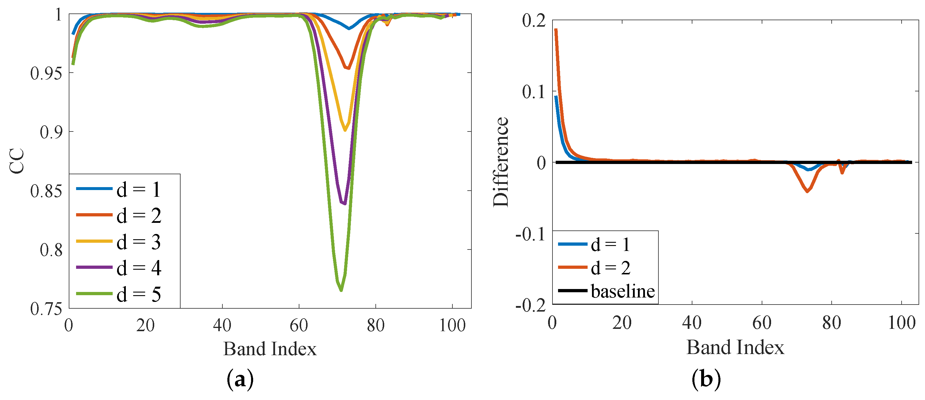
Correlation coefficients between neighboring bands in the LR HSIs were firstly measured to select the most proper interval. Figure 5a describes the variation of CC with the interval for the two-times down-sampled Pavia. It is noticed the CC decreased as the interval increased. This validated that the neighboring bands were highly correlated. However, as their interval became wider, their correlation coefficients decreased. Meanwhile, as the scaling factor increased, more high frequency details in the input LR HSIs were damaged, and the differences between different bands narrowed. Figure 5b plots the difference between the CC of the four-times down-sampled Pavia and that of the two-times down-sampled one, when interval was set as 1 and 2. It is noticed that the values of most differences were larger than 0. This validated that the bands in the four-times down-sampled HSIs were more correlated than those of the two-times down-sampled ones at the same interval. Thus, a larger interval can be set for the larger down-sampling factor, which would reduce the computational complexity with negligible performance loss.
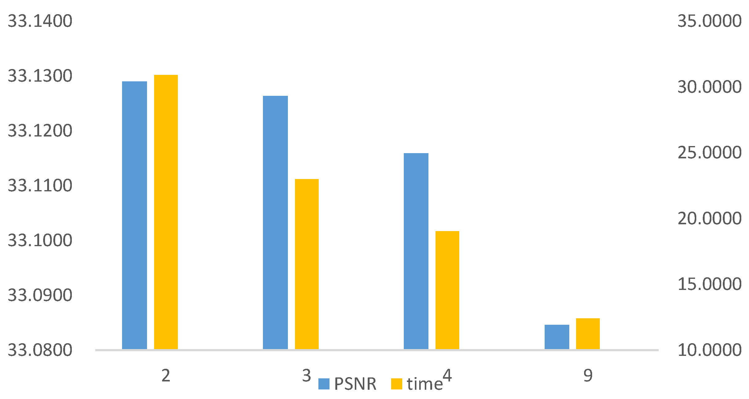
Table 1 is obtained by comparing the quality indices of the spectral-interpolated coarse HR HSIs with those of the IDN band-by-band super-resolved HR HSIs at different intervals. It is noticed that, at the same scaling factor, as the interval grew, the quality indices’ gap became bigger, which is consistent with what Figure 5a describes. Table 2 depicts the tendency of quality indices’ gap between the spectral-interpolated HR HSI and those of the IDN band-by-band super-resolved HR HSI at the same interval but different scaling factor. It is noticed that, with the same interval, the performance of the coarse HR HSI at scaling factor of 8 was closer to that of the IDN super-resolved than at the scaling factor of 4, and scaling factor of 4 was closer than scaling factor of 2, a phenomenon consistent with what shows in Figure 5b, which further validated the rationality of larger-interval setting for larger scale from a vertical perspective. In this way, setting for the “d” follows two principles: (1) for the HSIs with coarser spectral resolution, it is better to set a smaller “d”; and (2) for the HSIs with coarser spatial resolution, most high frequency differences between neighboring bands are lost, and their spectral correlation would be higher than the HSIs with finer spatial detail. A larger “d” can be set for these HSIs. Figure 6 shows the variation of PSNR and computation time with the band’s selection interval “d” for the Pavia University at the scaling factor of 2. It is noticed, as the “d” became larger, the computation time became less, but the PSNR of the reconstructed HSI became smaller, which validated our proposal’s tradeoff between high quality and high efficiency.
For the Pavia University HSI, there are 115 bands in the 430–860 nm, of which 12 bands were neglected and the remaining 103 bands were used for the experiment. There are 31 bands in the spectral range of 400–700 nm for the HSIs from the CAVE database, and 210 spectral bands covers the 400–2400 nm for the original Washington DC Mall HSI. In this way, from a horizontal perspective, under the same scaling factor, a larger interval was set for the spectrally more correlated Pavia University, and smaller interval is set for the Washington DC Mall and the HSIs from the CAVE database. Detailed interval settings for the experimental HSIs are displayed in Table 3.
3.2.1. Pavia University
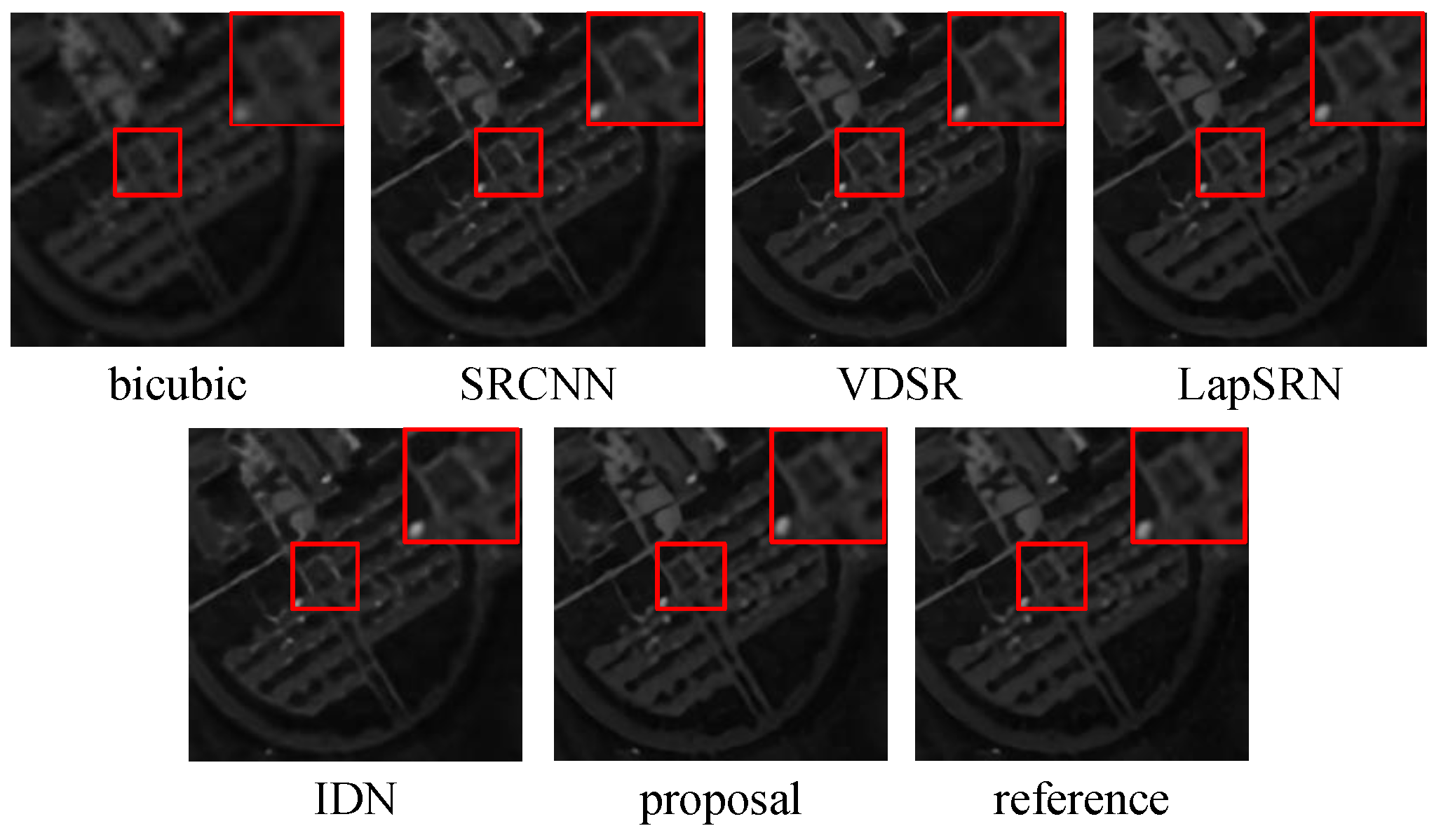
In Figure 7, we present a visual exhibition of the fourth band of the reconstructed Pavia University HSIs via various single based methods, with the scaling factor of 4.
As shown in Figure 7, the proposed method achieved a better spatial enhancement. Table 4 shows the averaged performance on the Pavia University HSI with comparison to the single-based methods. When compared with the SRCNN, VDSR and LapSRN, the proposed method achieved a better spatial enhancement of nearly 0.3–1 dB at the scaling factor of 2. In addition, the proposal only required about half the time of the IDN to achieve a comparable or better performance.
The proposed method achieved the best performance when the scaling factors were 4 and 8. The reason is that, as the scaling factor grew, less spatial information was contained in the input HSI. The performance of methods that super-resolve the LR HSI band by band would be severely damaged. The proposed method fully exploits the spatial-spectral information, achieving more acceptable performance.
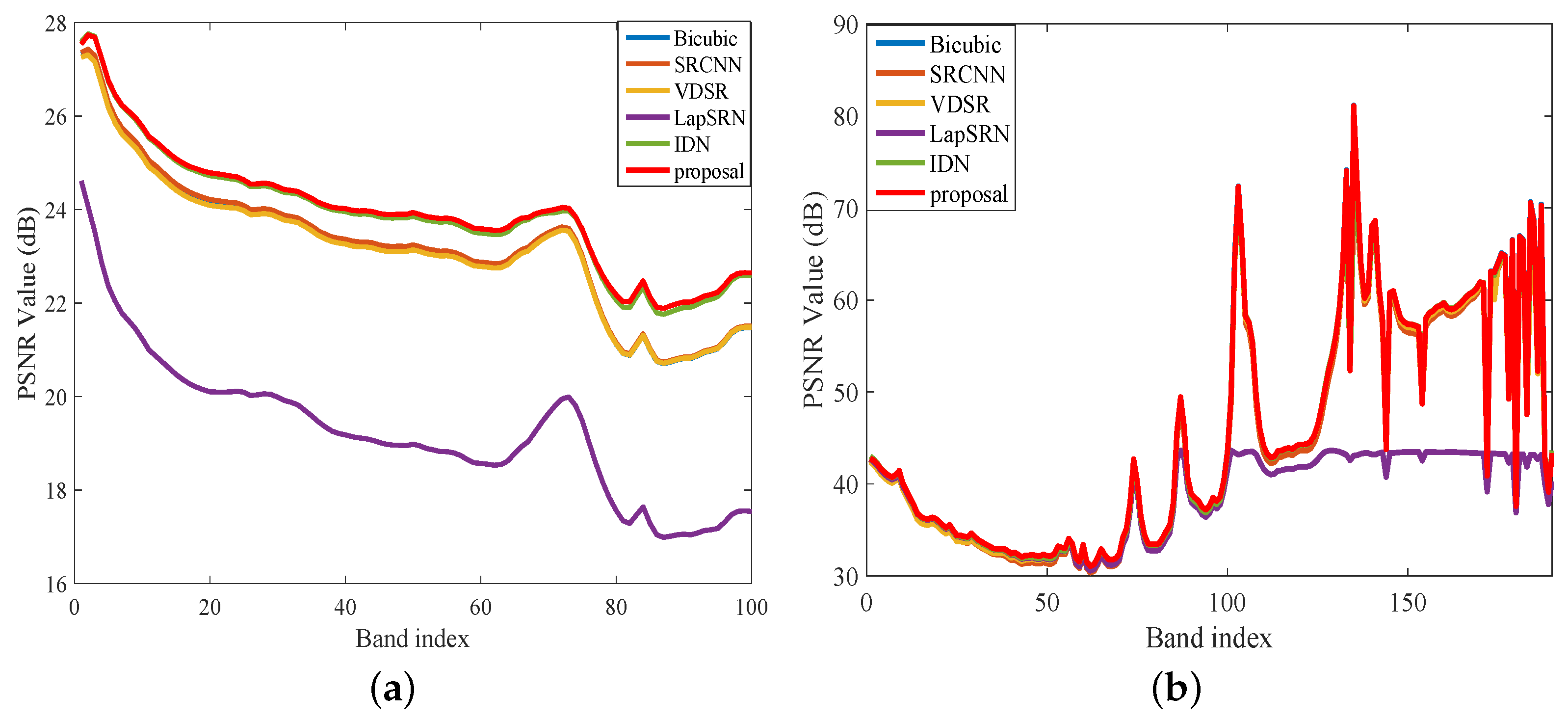
Figure 8a depicts the PSNRs of different bands in the 8× reconstructed Pavia University HSIs via different single based methods. It can be seen that the performance of the proposed method was superior to the other methods for each band.
3.2.2. Washington DC Mall
In Figure 9, we present a visual exhibition about the 90th band of the reconstructed Washington DC Mall via various single based methods, with the scaling factor of 4.
As shown in Figure 9, the proposed method achieved an HR HSI whose features are more distinct than the HSIs reconstructed by the other methods. Meanwhile, we randomly selected one point from the boundary of a region in the image and plotted its spectral curves (Figure 10). in Figure 10 “ref” represents the ground truth spectral curves. Because the spectral curve reconstructed by the IDN method seriously deviated from the reference one, we eliminated it in Figure 10 to have a better comparison with the other methods. The proposed method well preserved the spectral information. Contrary to the spectral curves reconstructed by the other methods, the locations of almost all the reflectance peaks and the reflectance troughs in the the spectral curve generated by the proposal are consistent with those of the reference curve, which ensures the correctness of their future applications.
Figure 8b depicts the PSNRs of different bands in the 8× reconstructed Washington DC Mall HSIs via different single-based methods. It can also be seen that the performance of the proposed method was superior to the other methods for each band.
Table 5 shows the averaged performance on the reconstructed Washington DC Mall with comparison to the other single-based methods. When compared with the SRCNN, VDSR and LapSRN, the proposal achieved a better spatial enhancement of nearly 0–0.5 dB at the scaling factor of 2.
At the scaling factors of 4 and 8, the proposal also achieved the best performance. As the selection interval for Washington DC Mall is smaller than that of Pavia University, the computational complexity’s superiority over the IDN was smaller than that for Pavia University, but still reduced about 40% at the scaling factor of 8.
3.2.3. Salinas
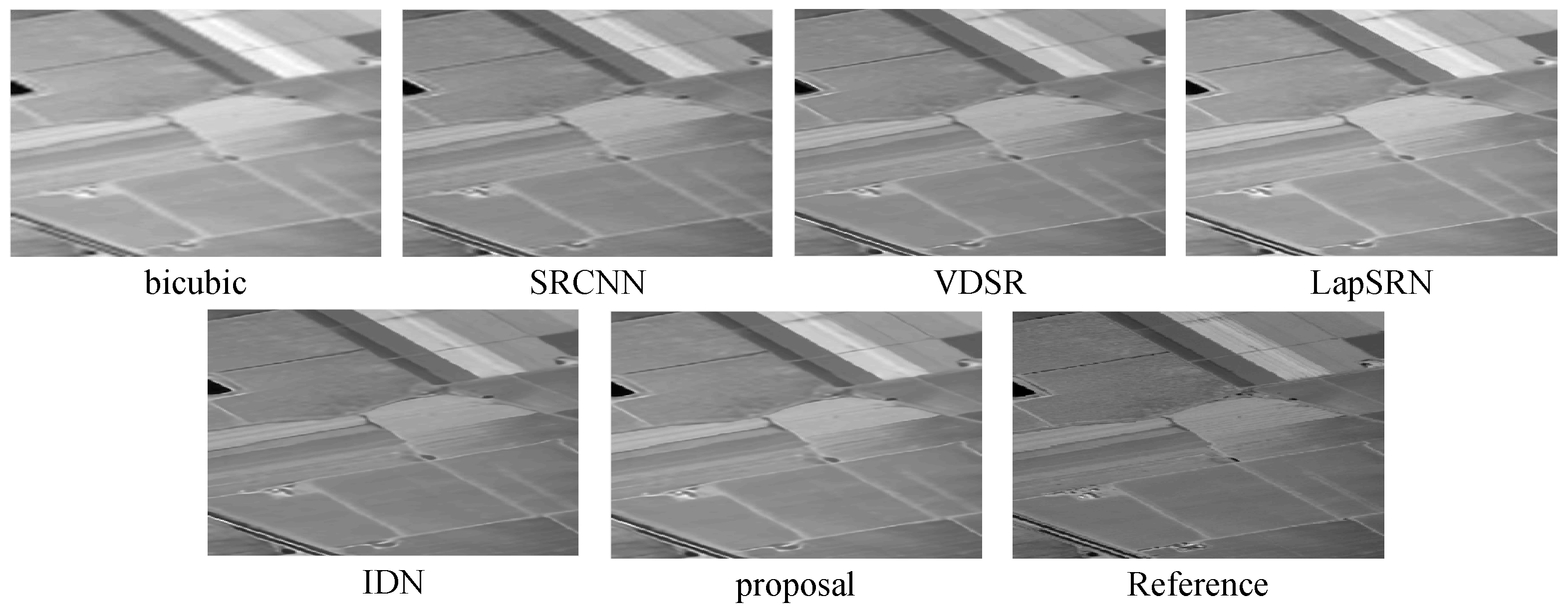
In Figure 11, visual exhibition about the 99th band of the reconstructed Salinas HSIs is presented, with the scaling factor set to 4.
As the land cover in Salinas is quite smooth, no big visual difference in the main body between different methods can be noticed. However, for the junction of different land covers, its geometric shape reconstructed by the proposal is much more distinct than that of the other methods. Figure 12a depicts the PSNRs of each band in the 4× reconstructed Salinas via different methods. According to the data in Figure 12a, the proposal achieved a better spatial enhancement performance on most bands for super-resolving the 4× down-sampled Salinas HSI.
Table 6 shows the averaged performance of the Salinas HSI at different scaling factors.
When compared with the SRCNN, VDSR, and LapSRN method, the proposal achieved a better spatial quality of nearly 0.06–0.74 dB at the scaling factor of 2. When it comes to the scaling factors of 4 and 8, the proposal achieved the best performance by utilizing the least time. It is demonstrated that the proposal also achieved an acceptable performance on the remote-sensing HSI with land cover typology, besides for the building typology.
3.2.4. Botswana
Figure 12b depicts the PSNRs of each band in the 8× reconstructed Botswana via different methods. The proposal achieveD the best PSNRs for most bands. Table 7 depicts the performance comparison with the alternative methods on the spaceborne Botswana. According to the data in Table 7, the IDN’s performance superiority over the proposal gradually diminishED. When IT comes to the scaling factor of 8, the proposal outperformED the IDN in less time. When combining Figure 12b with the data in Table 7, it is convincing that the proposal achieved high performance with high efficiency. In addition, from the data in Table 7, the computational complexity of VDSR and SRCNN was always stable for scaling factors 2, 4 and 8. For the IDN and the proposal, as the size of the input image decreased, less computational complexity was required, which is more practical. Both the experimental data of Salinas and Botswana demonstrated the proposal’s effectiveness on the HSIs of land cover typology.
3.2.5. Scene02
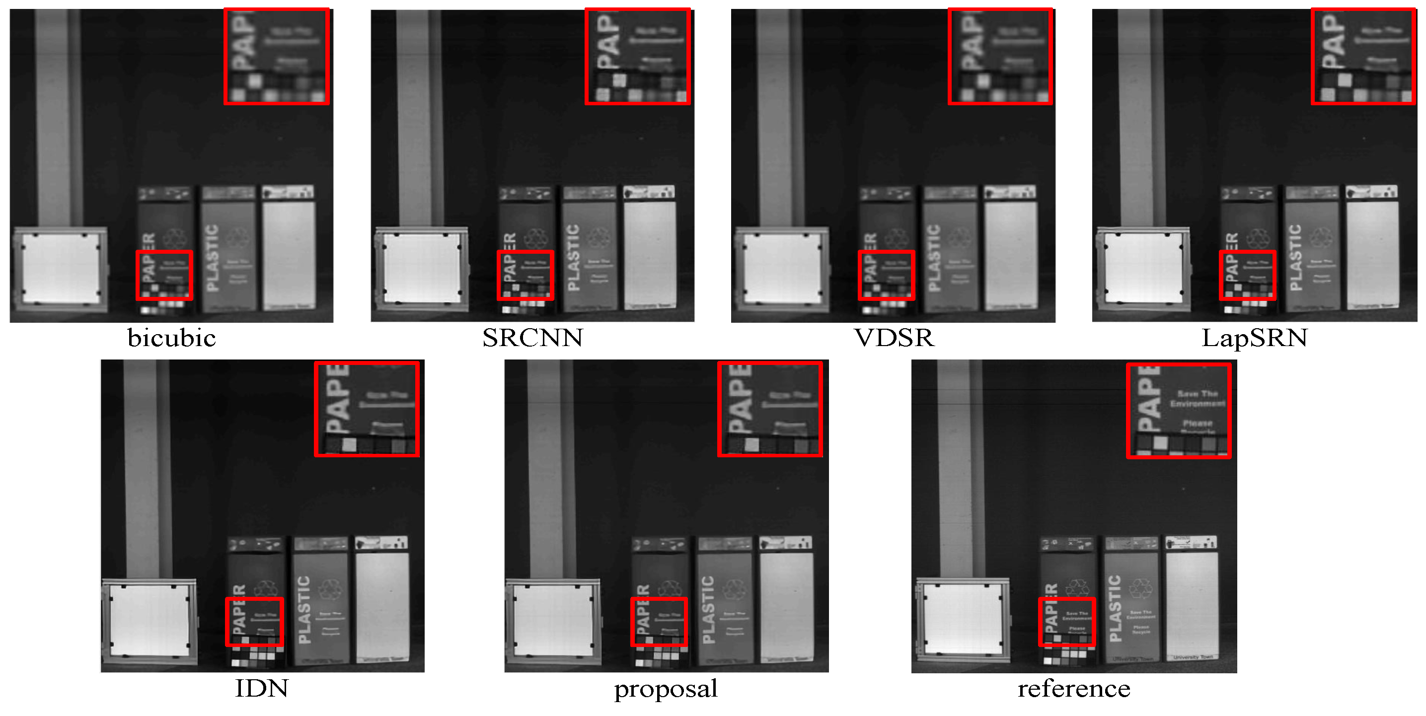
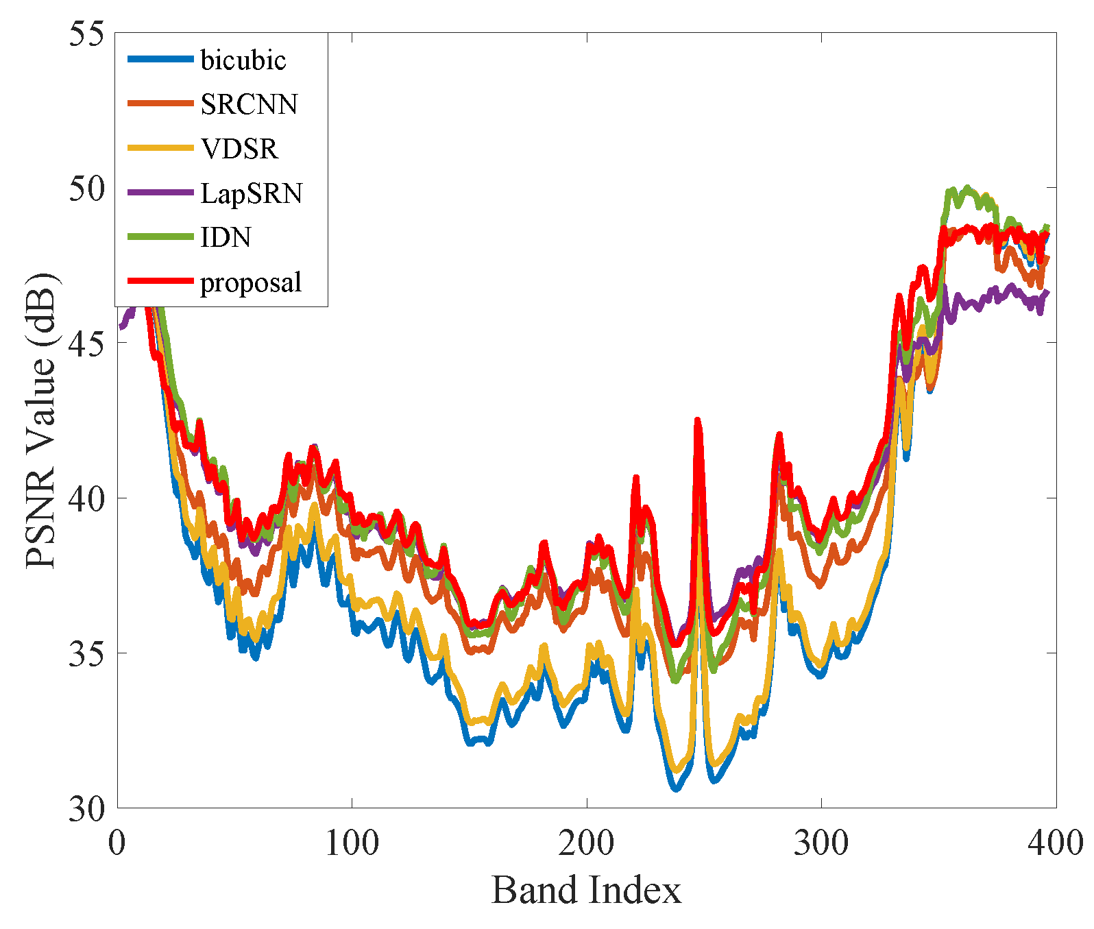
Although the spectral resolution of the Scene02 is finer than 10 nm per band, we still set small and conservative band interval for this HSI to obtain a better spatial enhancement. Figure 13 presents the visual exhibition about the 198th band for the 8× reconstructed Scene02. We amplified a square region that contains both the letter and the grid to make a comparison with the reconstructed HSIs via different methods. Both the contour of the letter and the boundary of the grid in the HSI reconstructed by the proposal are sharper than that of the other methods. Figure 14 depicts the PSNRs of each band in the 8× reconstructed Scene02. The proposal achieved the best performance for most of the single bands, especially for the bands locating at the middle wavelengths.
Table 8 shows the averaged performance on the reconstructed Scene02 via different methods. Limited by the memory, the running time of this HSI was much longer than the others, and the proposal achieved a significant computational reduction. This demonstrated that, as the image size grows, the proposal will achieve a notable computational advantage over the IDN.
3.2.6. CAVE Database
For the ground-based remote sensing HSIs in the CAVE database, their spatial quality is much finer than that of the other HSIs. In this case, according to the data in Table 9, the performance of super-resolving the HSI band by band via the IDN method was slightly better than that of the proposed method.
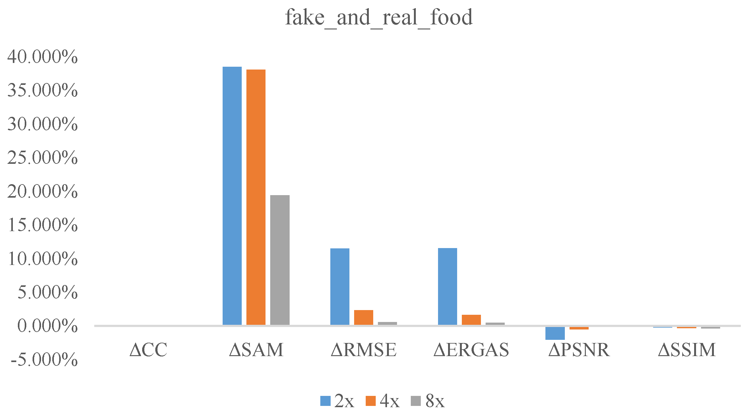
However, considering the input HSIs were generated by down-sampling from the original HSIs via bicubic interpolation, as the scaling factor grew, the spatial quality of the input HSIs decreased. Hence, it is rational to note that, as the scaling factor grew, the IDN’s superiority to the proposed method gradually diminished. Figure 15 plots the IDN’s superiority to the proposal on fake_and_real_food. It is noted that, as the scaling factor grew, the superiority gradually diminished and was next to 0, validating once again our proposal’s efficiency on remote sensing HSIs with poor spatial information. According to Kwan et al. [34], resolutions of most HSIs are limited to tens of meters, for which the proposed method would achieve a more appealing performance.
4. Conclusions
In this paper, an HSI super-resolution method is proposed by deeply utilizing the spatial-spectral information to reconstruct a high-resolution HSI from a low-resolution one. This method firstly incorporates different strategies for super-resolving the selected bands and the unselected ones. Compared with most of the existing single-based super-resolution methods, this scalable super-resolution operations greatly reduces the computational complexity with little performance degradation. Moreover, intra-fusion is operated to further improve the performance, which is more practical and does not require any auxiliary images. Through the proposed method, spatial-spectral information is fully exploited, and spatial details are well recovered. Experimental results and data analyses on both ground based and remote-sensing HSIs have demonstrated that the proposed method is especially suitable for dealing with the remote-sensing HSIs with poor spatial information.
Author Contributions
All authors made significant contributions to the manuscript. J.H. designed the research framework, analyzed the results and wrote the manuscript. M.Z. assisted in the preparation work and formal analysis. Y.L. supervised the framework design. All authors contributed to the editing and review of the manuscript.
Funding
This work was supported by the Natural Science Key Research Plan in Shaanxi Province of China (Program No.2016JZ001), PhD research startup foundation of Xi’an University of Technology (Program No.112/256081809), and Science and Technology Project of Xi’an City (No. 2017080CG/RC043(XALG011)).
Acknowledgments
The authors would like to take this opportunity to thank the editors and the reviewers for their detailed comments and suggestions.
Conflicts of Interest
The authors declare no conflict of interest.
References
- Zhang, F.; Du, B.; Zhang, L. Scene Classification via a Gradient Boosting Random Convolutional Network Framework. IEEE Trans. Geosci. Remote Sens. 2016, 54, 1793–1802. [Google Scholar] [CrossRef]
- Sun, W.; Du, Q. Graph-Regularized Fast and Robust Principal Component Analysis for Hyperspectral Band Selection. IEEE Trans. Geosci. Remote Sens. 2018, 56, 3185–3195. [Google Scholar] [CrossRef]
- Du, B.; Zhang, L. A Discriminative Metric Learning Based Anomaly Detection Method. IEEE Trans. Geosci. Remote Sens. 2014, 52, 6844–6857. [Google Scholar]
- Andrejchenko, V.; Liao, W.; Philips, W.; Scheunders, P. Decision Fusion Framework for Hyperspectral Image Classification Based on Markov and Conditional Random Fields. Remote Sens. 2019, 11, 624. [Google Scholar] [CrossRef]
- Sun, W.; Tian, L.; Xu, Y.; Du, B.; Du, Q. A Randomized Subspace Learning Based Anomaly Detector for Hyperspectral Imagery. Remote Sens. 2018, 10, 417. [Google Scholar] [Green Version]
- Dong, W.; Fu, F.; Shi, G.; Cao, X.; Wu, J.; Li, G.; Li, X. Hyperspectral Image Super-resolution via Non-negative Structured Sparse Representation. IEEE Trans. Image Process. 2016, 25, 2337–2351. [Google Scholar] [CrossRef] [PubMed]
- Fang, L.; Zhuo, H.; Li, S. Super-Resolution of Hyperspectral Image via Superpixel-Based Sparse Representation. Neurocomputing 2018, 273, 171–177. [Google Scholar] [CrossRef]
- Dian, R.; Fang, L.; Li, S. Hyperspectral Image Super-Resolution via Non-local Sparse Tensor Factorization. In Proceedings of the IEEE Conference on Computer Vision and Pattern Recognition, Honolulu, HI, USA, 21–26 July 2017. [Google Scholar]
- Kanatsoulis, C.I.; Fu, X.; Sidiropoulos, N.D.; Ma, W.K. Hyperspectral Super-Resolution: A Coupled Tensor Factorization Approach. IEEE Trans. Signal Process. 2018, 66, 6503–6517. [Google Scholar] [CrossRef] [Green Version]
- Zhang, L.; Wei, W.; Bai, C.; Gao, Y.; Zhang, Y. Exploiting Clustering Manifold Structure for Hyperspectral Imagery Super-Resolution. IEEE Trans. Image Process. 2018, 27, 5969–5982. [Google Scholar] [CrossRef]
- Han, X.H.; Shi, B.; Zheng, Y. Self-Similarity Constrained Sparse Representation for Hyperspectral Image Super-Resolution. IEEE Trans. Image Process. 2018, 27, 5625–5637. [Google Scholar] [CrossRef]
- Atkinson, P.M. Mapping sub-pixel vector boundaries from remotely sensed images. In Proceedings of the GISRUK ’96, Canterbury, UK, 10–12 April 1996; pp. 29–41. [Google Scholar]
- Irmak, H.; Akar, G.B.; Yuksel, S.E. A MAP-Based Approach for Hyperspectral Imagery Super-resolution. IEEE Trans. Image Process. 2018, 27, 2942–2951. [Google Scholar] [CrossRef]
- Arun, P.V.; Buddhiraju, K.M.; Porwal, A. CNN based sub-pixel mapping for hyperspectral images. Neurocomputing 2018, 311, 51–64. [Google Scholar] [CrossRef]
- Xu, X.; Tong, X.; Plaza, A.; Li, J.; Zhong, Y.; Xie, H.; Zhang, L. A New Spectral-Spatial Sub-Pixel Mapping Model for Remotely Sensed Hyperspectral Imagery. IEEE Trans. Geosci. Remote Sens. 2018, 56, 6763–6778. [Google Scholar] [CrossRef]
- Yuan, Y.; Zheng, X.; Lu, X. Hyperspectral Image Superresolution by Transfer Learning. IEEE J. Sel. Top. Appl. Earth Obs. Remote Sens. 2017, 10, 1963–1974. [Google Scholar] [CrossRef]
- He, Z.; Liu, L. Hyperspectral Image Super-Resolution Inspired by Deep Laplacian Pyramid Network. Remote Sens. 2018, 10, 1939. [Google Scholar] [CrossRef]
- Mei, S.; Yuan, X.; Ji, J.; Zhang, Y.; Wan, S.; Du, Q. Hyperspectral Image Spatial Super-Resolution via 3D Full Convolutional Neural Network. Remote Sens. 2017, 9, 1139. [Google Scholar] [CrossRef]
- Zheng, H.; Wang, X.; Gao, X. Fast and Accurate Single Image Super-Resolution via Information Distillation Network. In Proceedings of the IEEE Conference on Computer Vision and Pattern Recognition, Beijing, China, 20 August 2018; pp. 723–731. [Google Scholar]
- Yang, J.; Wright, J.; Huang, T.S.; Ma, Y. Image Super-Resolution Via Sparse Representation. IEEE Trans. Image Process. 2010, 19, 2861–2873. [Google Scholar] [CrossRef] [PubMed]
- Martin, D.; Fowlkes, C.; Tal, D.; Malik, J. A Database of Human Segmented Natural Images and its Application to Evaluating Segmentation Algorithms and Measuring Ecological Statistics. In Proceedings of the IEEE International Conference on Computer Vision, Vancouver, BC, Canada, 7–14 July 2001; Volume 2, pp. 416–423. [Google Scholar]
- Li, Y.; Xie, W.; Li, H. Hyperspectral image reconstruction by deep convolutional neural network for classification. Pattern Recognit. 2017, 63, 371–383. [Google Scholar] [CrossRef]
- Xu, Y.; Bo, D.; Fan, Z.; Zhang, L. Hyperspectral image classification via a random patches network. ISPRS J. Photogramm. Remote Sens. 2018, 142, 344–357. [Google Scholar] [CrossRef]
- Marrie, R.A.; Dawson, N.V.; Garland, A. Quantile regression and restricted cubic splines are useful for exploring relationships between continuous variables. J. Clin. Epidemiol. 2009, 62, 511–517. [Google Scholar] [CrossRef]
- Chang, C.I.; Du, Q. Estimation of number of spectrally distinct signal sources in hyperspectral imagery. IEEE Trans. Geosci. Remote Sens. 2004, 42, 608–619. [Google Scholar] [CrossRef]
- Yokoya, N.; Yairi, T.; Iwasaki, A. Coupled Nonnegative Matrix Factorization Unmixing for Hyperspectral and Multispectral Data Fusion. IEEE Trans. Geosci. Remote Sens. 2012, 50, 528–537. [Google Scholar] [CrossRef]
- Dong, C.; Loy, C.C.; He, K.; Tang, X. Image Super-Resolution Using Deep Convolutional Networks. IEEE Trans. Pattern Anal. Mach. Intell. 2015, 38, 295–307. [Google Scholar] [CrossRef] [Green Version]
- Kim, J.; Lee, J.K.; Lee, K.M. Accurate image super-resolution using very deep convolutional networks. In Proceedings of the IEEE Conference on Computer Vision and Pattern Recognition, Las Vegas, NV, USA, 27–30 June 2016; pp. 1646–1654. [Google Scholar]
- Lai, W.S.; Huang, J.B.; Ahuja, N.; Yang, M.H. Deep Laplacian Pyramid Networks for Fast and Accurate Super-Resolution. In Proceedings of the IEEE Conference on Computer Vision and Pattern Recognition, Honolulu, HI, USA, 21–26 July 2017; pp. 5835–5843. [Google Scholar]
- Lim, B.; Son, S.; Kim, H.; Nah, S.; Lee, K.M. Enhanced Deep Residual Networks for Single Image Super-Resolution. In Proceedings of the IEEE Conference on Computer Vision and Pattern Recognition, Honolulu, HI, USA, 21–26 July 2017; pp. 136–144. [Google Scholar]
- Yokoya, N. Texture-guided multisensor superresolution for remotely sensed images. Remote Sens. 2017, 9, 316. [Google Scholar] [CrossRef]
- Yuhas, R.; Goetz, A.F.H.; Boardman, J.W. Descrimination among semi-arid landscape endmembers using the Spectral Angle Mapper (SAM) algorithm. In Proceedings of the Summaries of the Third Annual JPL Airborne Geoscience Workshop, Pasadena, CA, USA, 1–5 June 1992; pp. 147–149. [Google Scholar]
- Loncan, L.; Almeida, L.B.; Bioucasdias, J.M.; Briottet, X.; Chanussot, J.; Dobigeon, N.; Fabre, S.; Liao, W.; Licciardi, G.A.; Simoes, M. Hyperspectral pansharpening: A review. IEEE Geosci. Remote Sens. Mag. 2015, 3, 27–46. [Google Scholar] [CrossRef]
- Kwan, C.; Choi, J.H.; Chan, S.H.; Zhou, J.; Budavari, B. A Super-Resolution and Fusion Approach to Enhancing Hyperspectral Images. Remote Sens. 2018, 10, 1416. [Google Scholar] [CrossRef]
Figure 1.
Workflow of the proposed method.

Figure 2.
Correlation between neighboring bands in the Pavia university scene.

Figure 3.
General architecture of the deep IDN.

Figure 4.
Visual exhibition of the HSIs used for validating the performance, in which all the gray images are generated by the 15th band in the corresponding HSIs.
Figure 4.
Visual exhibition of the HSIs used for validating the performance, in which all the gray images are generated by the 15th band in the corresponding HSIs.

Figure 5.
(a) CCs of two-times down-sampled Pavia with different intervals; and (b) CCs of four-times down-sampled Pavia minus that of two-times down-sampled Pavia with different intervals.
Figure 5.
(a) CCs of two-times down-sampled Pavia with different intervals; and (b) CCs of four-times down-sampled Pavia minus that of two-times down-sampled Pavia with different intervals.

Figure 6.
Variation of PSNR and computation time with “d” for the Pavia University at the scaling factor of 2.
Figure 6.
Variation of PSNR and computation time with “d” for the Pavia University at the scaling factor of 2.

Figure 7.
Visual exhibition of the fourth band created by the Pavia University HSIs, which are reconstructed by different single methods when scaling factor is 4.
Figure 7.
Visual exhibition of the fourth band created by the Pavia University HSIs, which are reconstructed by different single methods when scaling factor is 4.

Figure 8.
PSNRs of different bands in: (a) the 8× reconstructed Pavia University HSIs; an (b) 8× reconstructed Washington DC Mall HSIs via different single based methods.
Figure 8.
PSNRs of different bands in: (a) the 8× reconstructed Pavia University HSIs; an (b) 8× reconstructed Washington DC Mall HSIs via different single based methods.

Figure 9.
Visual exhibition of the 90th band created by the Washington DC Mall HSIs, which are reconstructed by different single methods when scaling factor is 4.
Figure 9.
Visual exhibition of the 90th band created by the Washington DC Mall HSIs, which are reconstructed by different single methods when scaling factor is 4.

Figure 10.
Spectral curves of the randomly selected point in the 8× reconstructed HR HSIs without IDN method.
Figure 10.
Spectral curves of the randomly selected point in the 8× reconstructed HR HSIs without IDN method.

Figure 11.
Visual exhibition of the 99th band created by the Salinas HSIs, which are reconstructed by different single methods when scaling factor is 4.
Figure 11.
Visual exhibition of the 99th band created by the Salinas HSIs, which are reconstructed by different single methods when scaling factor is 4.

Figure 12.
PSNRs of different bands in: (a) the 4× reconstructed Salinas HSIs; and (b) the 8× reconstructed Botswana via different single based methods
Figure 12.
PSNRs of different bands in: (a) the 4× reconstructed Salinas HSIs; and (b) the 8× reconstructed Botswana via different single based methods

Figure 13.
Visual exhibition of the 198th band created by the Scene02 HSIs, which are reconstructed by different single methods when scaling factor is 8.
Figure 13.
Visual exhibition of the 198th band created by the Scene02 HSIs, which are reconstructed by different single methods when scaling factor is 8.

Figure 14.
PSNRs for different bands in the 8× reconstructed Scene02 HSIs via different single based methods.
Figure 14.
PSNRs for different bands in the 8× reconstructed Scene02 HSIs via different single based methods.

Figure 15.
The gap of the performance between the IDN and the proposal on the “fake_and_real_food” HSI at scaling factors of 2, 4 and 8.
Figure 15.
The gap of the performance between the IDN and the proposal on the “fake_and_real_food” HSI at scaling factors of 2, 4 and 8.


Table 1.
Performance gap between and with different intervals.
| Interval d | Scaling Factor | CC | SAM | RMSE | ERGAS | PSNR | SSIM |
|---|---|---|---|---|---|---|---|
| 2× | −0.005% | 0.507% | 0.100% | 0.052% | −0.026% | −0.037% | |
| 4× | 0.003% | −0.017% | −0.003% | −0.048% | 0.001% | −0.017% | |
| 8× | 0.009% | −0.090% | −0.011% | −0.053% | 0.004% | −0.010% | |
| 2× | −0.014% | 1.239% | 0.223% | 0.283% | −0.058% | −0.071% | |
| 4× | −0.005% | 0.195% | 0.018% | 0.075% | −0.006% | −0.058% | |
| 8× | −0.005% | −0.060% | −0.006% | 0.054% | 0.002% | −0.056% | |
| 2× | −0.026% | 2.461% | 0.549% | 0.227% | −0.143% | −0.110% | |
| 4× | −0.008% | 0.599% | 0.083% | −0.228% | −0.027% | −0.073% | |
| 8× | 0.004% | 0.160% | 0.030% | −0.260% | −0.011% | −0.087% | |
| 2× | −0.134% | 14.244% | 3.408% | 3.390% | −0.879% | −0.648% | |
| 4× | −0.080% | 4.823% | 0.611% | 0.192% | −0.197% | −0.559% | |
| 8× | −0.047% | 1.254% | 0.155% | −0.283% | −0.057% | −0.499% |
Table 2.
Performance variation at the same intervals but with different scaling factors.
| Interval d | Scaling Factor | CC | SAM | RMSE | ERGAS | PSNR | SSIM |
|---|---|---|---|---|---|---|---|
| 4× − 2× | 0.008% | −0.525% | −0.104% | −0.100% | 0.027% | 0.020% | |
| 8× − 4× | 0.006% | −0.072% | −0.007% | −0.006% | 0.003% | 0.007% | |
| 4× − 2× | 0.009% | −1.043% | −0.204% | −0.209% | 0.052% | 0.013% | |
| 8× − 4× | 0.000% | −0.255% | −0.024% | −0.020% | 0.008% | 0.002% | |
| 4× − 2× | 0.017% | −1.862% | −0.466% | −0.455% | 0.117% | 0.037% | |
| 8× − 4× | 0.013% | −0.439% | −0.053% | −0.032% | 0.016% | −0.013% | |
| 4× − 2× | 0.053% | −9.421% | −2.797% | −3.198% | 0.682% | 0.089% | |
| 8× − 4× | 0.034% | −3.568% | −0.456% | −0.475% | 0.140% | 0.060% |
Table 3.
Interval d set for the HSI under different intervals.
| Pavia University | CAVE | Washington DC Mall | Salinas | Botswana | scene02 | |
|---|---|---|---|---|---|---|
| 2× | 3 | 2 | 2 | 2 | 2 | 2 |
| 4× | 9 | 3 | 3 | 3 | 3 | 3 |
| 8× | 9 | 3 | 3 | 3 | 3 | 3 |
Table 4.
Comparison with single-based methods on all the bands of the Pavia University.
| Scaling Factor | Algorithm | CC | SAM | RMSE | ERGAS | PSNR | SSIM | Time (s) |
|---|---|---|---|---|---|---|---|---|
| 2× | Bicubic | 0.9478 | 4.1099 | 0.0312 | 10.2627 | 30.1239 | 0.9024 | 0.0113 * |
| SRCNN | 0.9670 | 3.8253 | 0.0246 | 8.0368 | 32.1771 | 0.9359 | 146.4056 | |
| VDSR | 0.9715 | 3.6195 | 0.0229 | 7.4459 | 32.8153 | 0.9449 | 53.2367 | |
| LapSRN | 0.9710 | 3.4385 | 0.0231 | 7.4874 | 32.7146 | 0.9457 | 81.1535 | |
| IDN | 0.9737 | 3.4503 | 0.0219 | 7.1422 | 33.1886 | 0.9503 | 47.5715 | |
| Proposal | 0.9731 | 3.5608 | 0.0221 | 7.2108 | 33.1264 | 0.9482 | 22.9895 | |
| 4× | Bicubic | 0.8632 | 6.2994 | 0.0508 | 8.0125 | 25.8874 | 0.7182 | 0.0045 * |
| SRCNN | 0.8802 | 6.1240 | 0.0473 | 7.5101 | 26.5115 | 0.7551 | 135.9020 | |
| VDSR | 0.8814 | 6.3009 | 0.0470 | 7.4961 | 26.5508 | 0.7613 | 50.8616 | |
| LapSRN | 0.8890 | 5.7116 | 0.0458 | 7.2154 | 26.7848 | 0.7776 | 24.0806 | |
| IDN | 0.8906 | 5.7168 | 0.0452 | 7.1654 | 26.8934 | 0.7831 | 11.8475 | |
| Proposal | 0.8907 | 5.6563 | 0.0452 | 7.1565 | 26.9029 | 0.7837 | 6.6167 | |
| 8× | Bicubic | 0.7272 | 9.2785 | 0.0711 | 5.4737 | 22.9664 | 0.5081 | 0.0105 * |
| SRCNN | 0.7292 | 9.2148 | 0.0707 | 5.4644 | 23.0061 | 0.5107 | 152.1849 | |
| VDSR | 0.7232 | 9.3343 | 0.0713 | 5.4955 | 22.9329 | 0.5030 | 50.6967 | |
| LapSRN | 0.7489 | 9.0115 | 0.0682 | 5.3306 | 23.3192 | 0.5289 | 19.3687 | |
| IDN | 0.7709 | 8.6351 | 0.0652 | 5.0774 | 23.7182 | 0.5710 | 13.9152 | |
| Proposal | 0.7739 | 8.2311 | 0.0646 | 5.0448 | 23.7915 | 0.5759 | 5.4009 |
The asterisk * in the tables denote the best performance for the time measurement among all the methods. However, limited by its poor performance, we eliminated it from the comparison and make another time comparison among the other methods, in which we emphases the next least time in a bold format.
Table 5.
Comparison with single-based methods on all the bands of the Washington DC Mall.
| Scaling Factor | Algorithm | CC | SAM | RMSE | ERGAS | PSNR | SSIM | Time (s) |
|---|---|---|---|---|---|---|---|---|
| 2× | Bicubic | 0.9146 | 3.9147 | 0.0067 | 132.1512 | 43.4877 | 0.9755 | 0.1141 * |
| SRCNN | 0.9278 | 4.3988 | 0.0068 | 37.7941 | 43.3780 | 0.9741 | 1368.6865 | |
| VDSR | 0.9248 | 4.5313 | 0.0064 | 60.8111 | 43.8360 | 0.9779 | 467.5891 | |
| LapSRN | 0.9064 | 3.4886 | 0.0056 | 137.4491 | 45.0408 | 0.9828 | 187.9704 | |
| IDN | 0.9472 | 3.4280 | 0.0054 | 95.1557 | 45.2791 | 0.9837 | 438.5749 | |
| Proposal | 0.9190 | 3.4311 | 0.0056 | 79.2654 | 45.0717 | 0.9833 | 286.9364 | |
| 4× | Bicubic | 0.8255 | 6.5297 | 0.0107 | 72.3078 | 39.4441 | 0.9374 | 0.0991 * |
| SRCNN | 0.8186 | 7.1202 | 0.0108 | 239.5115 | 39.3414 | 0.9329 | 1268.5417 | |
| VDSR | 0.8138 | 7.7250 | 0.0116 | 47.0651 | 38.7003 | 0.9316 | 468.6285 | |
| LapSRN | 0.7216 | 7.2031 | 0.0106 | 2533.9007 | 39.4647 | 0.9289 | 225.3079 | |
| IDN | 0.8514 | 6.4612 | 0.0101 | 46.0912 | 39.8993 | 0.9443 | 64.0762 | |
| Proposal | 0.8310 | 6.2754 | 0.0101 | 60.8714 | 39.9268 | 0.9447 | 69.6417 | |
| 8× | Bicubic | 0.7181 | 9.0515 | 0.0144 | 35.0310 | 36.8363 | 0.9011 | 0.0807 * |
| SRCNN | 0.6821 | 9.8476 | 0.0149 | 681.0136 | 36.5157 | 0.8959 | 1365.1717 | |
| VDSR | 0.7095 | 9.1466 | 0.0144 | 24.4473 | 36.8106 | 0.9004 | 469.7174 | |
| LapSRN | 0.5078 | 11.9678 | 0.0152 | 7.9641 | 36.3660 | 0.8064 | 169.2427 | |
| IDN | 0.7213 | 9.0498 | 0.0140 | 29.7419 | 37.0500 | 0.9054 | 137.0598 | |
| Proposal | 0.7219 | 8.7892 | 0.0138 | 34.7061 | 37.1833 | 0.9069 | 85.9309 |
The asterisk * in the tables denote the best performance for the time measurement among all the methods. However, limited by its poor performance, we eliminated it from the comparison and make another time comparison among the other methods, in which we emphases the next least time in a bold format.
Table 6.
Comparison with single-based methods on all the bands of the Salinas.
| Scaling Factor | Algorithm | CC | SAM | RMSE | ERGAS | PSNR | SSIM | Time (s) |
|---|---|---|---|---|---|---|---|---|
| 2× | Bicubic | 0.9833 | 0.8145 | 0.0073 | 2.8216 | 42.6932 | 0.9881 | 0.0875 * |
| SRCNN | 0.9845 | 0.7838 | 0.006044008 | 2.9319 | 44.3735 | 0.9910 | 478.2165 | |
| VDSR | 0.9855 | 0.7296 | 0.0056 | 2.6816 | 45.0141 | 0.9923 | 285.4522 | |
| LapSRN | 0.9851 | 0.7027 | 0.0056 | 2.7610 | 45.0584 | 0.9927 | 93.4594 | |
| IDN | 0.9899 | 0.6862 | 0.0054 | 2.1774 | 45.2783 | 0.9930 | 153.7260 | |
| Proposal | 0.9831 | 0.7937 | 0.0055 | 2.7174 | 45.1159 | 0.9927 | 142.5217 | |
| 4× | Bicubic | 0.9618 | 1.3393 | 0.0126 | 2.1649 | 38.0198 | 0.9671 | 0.0656 * |
| SRCNN | 0.9647 | 1.2653 | 0.0105 | 2.3292 | 39.5892 | 0.9733 | 474.2595 | |
| VDSR | 0.9669 | 1.2002 | 0.0098 | 2.0414 | 40.2124 | 0.9773 | 288.5284 | |
| LapSRN | 0.9595 | 1.1927 | 0.0095 | 4.7102 | 40.4442 | 0.9774 | 112.7037 | |
| IDN | 0.9709 | 1.1292 | 0.0095 | 1.9040 | 40.4857 | 0.9796 | 40.9700 | |
| Proposal | 0.9690 | 1.2063 | 0.0095 | 1.9272 | 40.4898 | 0.9799 | 28.2351 | |
| 8× | Bicubic | 0.9325 | 1.9881 | 0.0177 | 1.4398 | 35.0562 | 0.9469 | 0.0624 * |
| SRCNN | 0.9376 | 1.8607 | 0.0155 | 1.4626 | 36.2152 | 0.9509 | 493.3159 | |
| VDSR | 0.9328 | 1.9848 | 0.0176 | 1.4311 | 35.0677 | 0.9470 | 278.9407 | |
| LapSRN | 0.9164 | 1.8910 | 0.0146 | 2.2318 | 36.7126 | 0.9457 | 75.7862 | |
| IDN | 0.9457 | 1.5874 | 0.0139 | 1.2972 | 37.1265 | 0.9600 | 47.2434 | |
| Proposal | 0.9466 | 1.6081 | 0.0139 | 1.2685 | 37.1643 | 0.9608 | 23.1352 |
The asterisk * in the tables denote the best performance for the time measurement among all the methods. However, limited by its poor performance, we eliminated it from the comparison and make another time comparison among the other methods, in which we emphases the next least time in a bold format.
Table 7.
Comparison with single-based methods on all the bands of the spaceborne Botswana.
| Scaling Factor | Algorithm | CC | SAM | RMSE | ERGAS | PSNR | SSIM | Time (s) |
|---|---|---|---|---|---|---|---|---|
| 2× | Bicubic | 0.9749 | 1.5638 | 0.0027 | 3.2346 | 51.4286 | 0.9936 | 0.1697 * |
| SRCNN | 0.9726 | 1.7866 | 0.0027 | 4.7684 | 51.3234 | 0.9930 | 1841.7661 | |
| VDSR | 0.9733 | 1.7494 | 0.0026 | 3.6777 | 51.5523 | 0.9938 | 665.7049 | |
| LapSRN | 0.9613 | 1.5565 | 0.0024 | 4.8883 | 52.2804 | 0.9947 | 215.5832 | |
| IDN | 0.9790 | 1.5057 | 0.0025 | 2.9631 | 52.1939 | 0.9946 | 382.3559 | |
| Proposal | 0.9750 | 1.6567 | 0.0025 | 3.3550 | 52.1000 | 0.9945 | 194.3229 | |
| 4× | Bicubic | 0.9360 | 2.2719 | 0.0041 | 2.5785 | 47.6567 | 0.9852 | 0.1545 * |
| SRCNN | 0.9264 | 2.7466 | 0.0044 | 4.0511 | 47.1981 | 0.9830 | 1837.1380 | |
| VDSR | 0.9333 | 2.4853 | 0.0043 | 2.6621 | 47.3913 | 0.9845 | 664.6281 | |
| LapSRN | 0.8693 | 2.8898 | 0.0044 | 17.7117 | 47.0433 | 0.9784 | 260.7957 | |
| IDN | 0.9359 | 2.3089 | 0.0041 | 2.5866 | 47.7809 | 0.9857 | 100.8897 | |
| Proposal | 0.9348 | 2.3693 | 0.0041 | 2.6304 | 47.7727 | 0.9857 | 110.1546 | |
| 8× | Bicubic | 0.8849 | 2.8682 | 0.0054 | 1.7057 | 45.3479 | 0.9776 | 0.1050 * |
| SRCNN | 0.8768 | 3.3473 | 0.0056 | 1.8735 | 45.0566 | 0.9743 | 1937.2458 | |
| VDSR | 0.8849 | 2.8933 | 0.0054 | 1.7005 | 45.3436 | 0.9774 | 649.2971 | |
| LapSRN | 0.7188 | 5.6478 | 0.0068 | 4.4614 | 43.3178 | 0.9264 | 181.4325 | |
| IDN | 0.8849 | 2.8926 | 0.0053 | 1.7069 | 45.4540 | 0.9780 | 111.4147 | |
| Proposal | 0.8842 | 2.9210 | 0.0053 | 1.7239 | 45.4730 | 0.9780 | 95.1863 |
The asterisk * in the tables denote the best performance for the time measurement among all the methods. However, limited by its poor performance, we eliminated it from the comparison and make another time comparison among the other methods, in which we emphases the next least time in a bold format.
Table 8.
Comparison with single-based methods on all the bands of the ground-based Scene02.
| Scaling Factor | Algorithm | CC | SAM | RMSE | ERGAS | PSNR | SSIM | Time (s) |
|---|---|---|---|---|---|---|---|---|
| 2× | Bicubic | 0.9893 | 1.3497 | 0.0038 | 2.5991 | 48.3610 | 0.9893 | 1.7652 * |
| SRCNN | 0.9883 | 1.3526 | 0.0034 | 2.5906 | 49.3194 | 0.9902 | 22,196.9520 | |
| VDSR | 0.9894 | 1.8098 | 0.0033 | 2.4903 | 49.6012 | 0.9906 | 7087.1100 | |
| LapSRN | 0.9894 | 1.2918 | 0.0033 | 2.5009 | 49.6579 | 0.9907 | 2453.7132 | |
| IDN | 0.9891 | 1.5624 | 0.0032 | 3.3076 | 49.8186 | 0.9872 | 31,600.1253 | |
| Proposal | 0.9864 | 1.6264 | 0.0041 | 3.3196 | 47.7878 | 0.9871 | 16,385.2456 | |
| 4× | Bicubic | 0.9882 | 1.6586 | 0.0085 | 1.6540 | 41.4224 | 0.9758 | 2.3729 * |
| SRCNN | 0.9884 | 1.6882 | 0.0066 | 1.5514 | 43.6492 | 0.9797 | 19,569.4504 | |
| VDSR | 0.9887 | 1.6641 | 0.0070 | 1.5190 | 43.0552 | 0.9801 | 7088.5478 | |
| LapSRN | 0.9879 | 1.6623 | 0.0065 | 1.6303 | 43.7951 | 0.9806 | 2967.9555 | |
| IDN | 0.9890 | 1.6544 | 0.0067 | 1.4828 | 43.5267 | 0.9810 | 1043.8702 | |
| Proposal | 0.9853 | 1.8455 | 0.0069 | 1.7098 | 43.2549 | 0.9800 | 837.5474 | |
| 8× | Bicubic | 0.9813 | 1.9210 | 0.0170 | 1.2834 | 35.4108 | 0.9522 | 1.3983 * |
| SRCNN | 0.9840 | 1.9561 | 0.0123 | 2.1736 | 38.1769 | 0.9631 | 20,230.4446 | |
| VDSR | 0.9823 | 1.9240 | 0.0159 | 2.4345 | 35.9543 | 0.9543 | 7078.2086 | |
| LapSRN | 0.9827 | 1.9827 | 0.0110 | 2.2127 | 39.2082 | 0.9661 | 1995.0681 | |
| IDN | 0.9855 | 1.9431 | 0.0112 | 1.9610 | 39.0254 | 0.9682 | 1263.6725 | |
| Proposal | 0.9825 | 2.0155 | 0.0108 | 2.0875 | 39.3101 | 0.9687 | 794.5077 |
The asterisk * in the tables denote the best performance for the time measurement among all the methods. However, limited by its poor performance, we eliminated it from the comparison and make another time comparison among the other methods, in which we emphases the next least time in a bold format.
Table 9.
Comparison with single-based methods on all the bands of the two HSIs from the CAVE database.
Table 9.
Comparison with single-based methods on all the bands of the two HSIs from the CAVE database.
| Scaling Factor | Algorithm | CC | SAM | RMSE | ERGAS | PSNR | SSIM | Time (s) | |
|---|---|---|---|---|---|---|---|---|---|
| flowers | 2× | Bicubic | 0.9984 | 2.2374 | 0.0077 | 4.7471 | 42.2459 | 0.9903 | 0.0336 * |
| SRCNN | 0.9989 | 3.4207 | 0.0063 | 4.1371 | 44.0429 | 0.9909 | 291.4331 | ||
| VDSR | 0.9947 | 3.3941 | 0.0147 | 8.8671 | 36.6603 | 0.9667 | 104.7910 | ||
| LapSRN | 0.9994 | 2.5744 | 0.0048 | 3.0139 | 46.4618 | 0.9951 | 41.9354 | ||
| IDN | 0.9994 | 1.8481 | 0.0045 | 2.8960 | 46.8784 | 0.9957 | 99.0016 | ||
| Proposal | 0.9992 | 2.5642 | 0.0051 | 3.4598 | 45.9336 | 0.9939 | 66.4343 | ||
| 4× | Bicubic | 0.9927 | 3.7917 | 0.0172 | 5.1599 | 35.2872 | 0.9563 | 0.0304 * | |
| SRCNN | 0.9939 | 5.1345 | 0.0152 | 4.7506 | 36.3380 | 0.9598 | 294.0630 | ||
| VDSR | 0.9923 | 4.1526 | 0.0170 | 5.3323 | 35.3768 | 0.9507 | 105.5385 | ||
| LapSRN | 0.9955 | 6.5766 | 0.0133 | 4.1492 | 37.5383 | 0.9631 | 49.7823 | ||
| IDN | 0.9959 | 2.9697 | 0.0128 | 3.8981 | 37.8402 | 0.9733 | 24.3753 | ||
| Proposal | 0.9957 | 4.3377 | 0.0129 | 3.9524 | 37.7836 | 0.9711 | 21.0441 | ||
| 8× | Bicubic | 0.9765 | 6.3186 | 0.0308 | 4.5832 | 30.2423 | 0.8855 | 0.0282 * | |
| SRCNN | 0.9766 | 7.6651 | 0.0300 | 4.6077 | 30.4565 | 0.8838 | 304.0369 | ||
| VDSR | 0.9765 | 6.2937 | 0.0305 | 4.5635 | 30.3116 | 0.8876 | 104.5376 | ||
| LapSRN | 0.9833 | 12.2898 | 0.0259 | 3.7601 | 31.7479 | 0.8482 | 37.3913 | ||
| IDN | 0.9851 | 4.6558 | 0.0247 | 3.6355 | 32.1417 | 0.9249 | 28.4277 | ||
| Proposal | 0.9849 | 6.6257 | 0.0248 | 3.6574 | 32.1266 | 0.9221 | 20.1004 | ||
| fake_and_real_food | 2× | Bicubic | 0.9974 | 2.2996 | 0.0076 | 7.4718 | 42.4225 | 0.9905 | 0.0334 * |
| SRCNN | 0.9979 | 2.7596 | 0.0068 | 6.6207 | 43.3160 | 0.9907 | 277.1336 | ||
| VDSR | 0.9982 | 2.5201 | 0.0063 | 6.1294 | 44.0514 | 0.9919 | 105.6183 | ||
| LapSRN | 0.9988 | 2.1301 | 0.0052 | 5.0164 | 45.7448 | 0.9944 | 41.4651 | ||
| IDN | 0.9989 | 1.8804 | 0.0050 | 4.7845 | 46.0583 | 0.9950 | 98.3872 | ||
| Proposal | 0.9986 | 2.6043 | 0.0056 | 5.3368 | 45.1141 | 0.9927 | 68.0450 | ||
| 4× | Bicubic | 0.9898 | 3.5765 | 0.0153 | 7.3000 | 36.3087 | 0.9641 | 0.0230 * | |
| SRCNN | 0.9931 | 4.0173 | 0.0127 | 5.8726 | 37.8964 | 0.9701 | 296.6172 | ||
| VDSR | 0.9915 | 4.0963 | 0.0140 | 6.5949 | 37.0649 | 0.9666 | 104.8076 | ||
| LapSRN | 0.9953 | 3.9114 | 0.0105 | 5.0602 | 39.5662 | 0.9761 | 49.7072 | ||
| IDN | 0.9954 | 2.8206 | 0.0104 | 4.8477 | 39.6913 | 0.9816 | 24.5117 | ||
| Proposal | 0.9951 | 3.8955 | 0.0106 | 4.9266 | 39.4917 | 0.9781 | 22.3028 | ||
| 8× | Bicubic | 0.9704 | 5.4984 | 0.0270 | 5.9880 | 31.3585 | 0.9111 | 0.0305 * | |
| SRCNN | 0.9746 | 6.5774 | 0.0254 | 5.4663 | 31.8919 | 0.9150 | 298.1715 | ||
| VDSR | 0.9717 | 5.5900 | 0.0263 | 5.8597 | 31.6012 | 0.9130 | 104.9534 | ||
| LapSRN | 0.9843 | 8.2559 | 0.0200 | 4.1520 | 33.9588 | 0.9114 | 37.2533 | ||
| IDN | 0.9864 | 4.0106 | 0.0184 | 4.0935 | 34.6995 | 0.9534 | 28.1883 | ||
| Proposal | 0.9860 | 4.7878 | 0.0185 | 4.1123 | 34.6518 | 0.9498 | 20.3372 |
The asterisk * in the tables denote the best performance for the time measurement among all the methods. However, limited by its poor performance, we eliminated it from the comparison and make another time comparison among the other methods, in which we emphases the next least time in a bold format.
© 2019 by the authors. Licensee MDPI, Basel, Switzerland. This article is an open access article distributed under the terms and conditions of the Creative Commons Attribution (CC BY) license (http://creativecommons.org/licenses/by/4.0/).
Share and Cite
MDPI and ACS Style
Hu, J.; Zhao, M.; Li, Y. Hyperspectral Image Super-Resolution by Deep Spatial-Spectral Exploitation. Remote Sens. 2019, 11, 1229. https://0-doi-org.brum.beds.ac.uk/10.3390/rs11101229
AMA Style
Hu J, Zhao M, Li Y. Hyperspectral Image Super-Resolution by Deep Spatial-Spectral Exploitation. Remote Sensing. 2019; 11(10):1229. https://0-doi-org.brum.beds.ac.uk/10.3390/rs11101229
Chicago/Turabian StyleHu, Jing, Minghua Zhao, and Yunsong Li. 2019. "Hyperspectral Image Super-Resolution by Deep Spatial-Spectral Exploitation" Remote Sensing 11, no. 10: 1229. https://0-doi-org.brum.beds.ac.uk/10.3390/rs11101229
Note that from the first issue of 2016, this journal uses article numbers instead of page numbers. See further details here.