Higher-Order Conditional Random Fields-Based 3D Semantic Labeling of Airborne Laser-Scanning Point Clouds


 , , ,
, , ,
Abstract
:1. Introduction
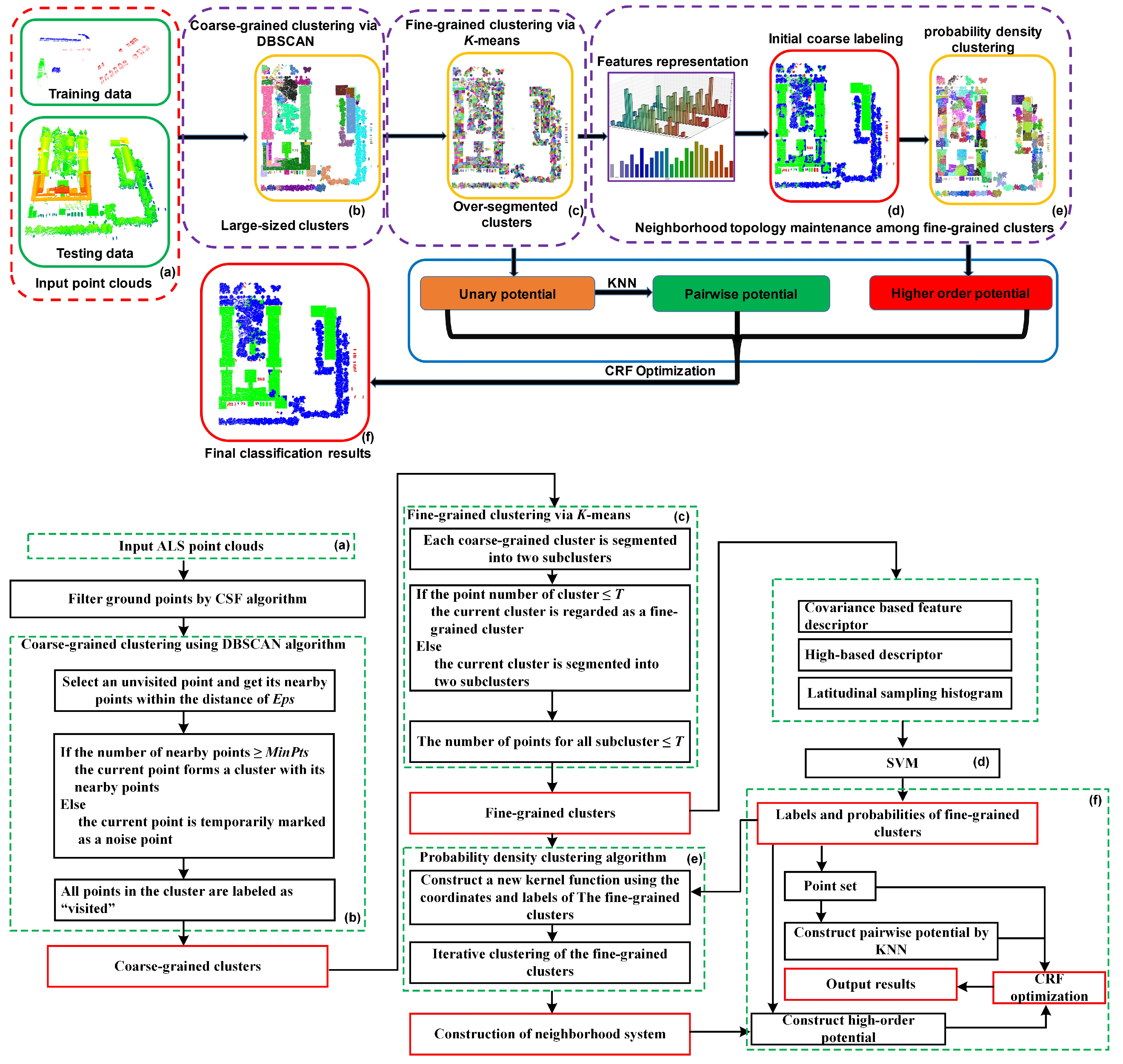
- Hierarchical Point Cluster Generation: We propose a multilevel clustering point set construction method. The first-level clustering uses a density clustering method to aggregate the points belonging to the same kind of object into a coarse cluster set. The second-level clustering uses the classic K-means algorithm to over-segment the coarse cluster set into a fine cluster set, from which the point set of the minimum processing unit is constructed. The third-level clustering uses the proposed probability density clustering method to construct a cluster set at a high-level scale, i.e., the third-level cluster set includes one-to-many relationships with the second-level cluster set. The multilevel clusters commonly provide greater use of contextual information, thus improving the accuracy of clustering labeling.
- Cluster Topology Maintenance Strategy: We present a strategy of constructing a neighborhood system among clusters by turning the problem of topology maintenance of clusters into a clustering problem based on the proposed probability density clustering method.
- Higher-Order Energy Function: We propose a higher-order CRF energy function that considers the constraints of the unary potential, the pairwise potential, and the higher-order potential defined over cliques consisting of more than two clusters.
2. Methodology
2.1. Materials
2.2. Coarse-Grained Clustering Using DBSCAN
- Core Point: Any point p with several neighborhood points that is greater than or equal to is regarded as a core point.
- Border Point: For any point p, if the number of its neighbors is less than , it belongs to the -neighborhood of some core points.
- Noise Point: If a point is neither a core point nor a border point, then it is called a noise point or an outlier.
2.3. Fine-Grained Clustering Using K-Means
- (1)
- Choose an arbitrary cluster from the coarse-grained cluster set as a processing unit and then randomly choose points as the beginning centroids, i.e., = .
- (2)
- Assign the point clouds within to their associated centroids according to the criterion of the minimum Euclidean metric from a point to its associated centroid. After t iterations, we obtain:where represents the minimum Euclidean metric between two points.
- (3)
- Update the centroid of each class:
- (4)
- Repeat steps (2) to (3) until the centroid locations remain stable, i.e.,
2.4. Neighborhood Relationship Maintenance between Fine-Grained Clusters
2.4.1. Initial Coarse Labeling of Fine-Grained Clusters
2.4.2. Creation of Neighborhood System
- (1)
- Select an initial cluster center from the unlabeled set X, and set its class as the current cluster’s label.
- (2)
- Label the centroids of the cluster in . If they are consistent with the label of the current centroid, we update the accumulator.
- (3)
- Calculate the deviation vector using Equation (4) and update the center of the current cluster.
- (4)
- Repeat steps (2) to (3) until the mean deviation is less than a threshold, i.e., .
- (5)
- Determine whether the Euclidean metric from the current cluster’s center to the existing center is less than . If it is true, these two clusters need to be merged, otherwise the current cluster is regarded as a new cluster.
- (6)
- Execute the steps from (1) to (5) until all the centroids of the clusters have been assigned a specific label.
- (7)
- For each centroid of a cluster, we assign the label with the highest frequency of visits as an associated label.
2.5. CRF Classification with Higher-Order Potentials
3. Performance Evaluation and Discussion
3.1. Implementation
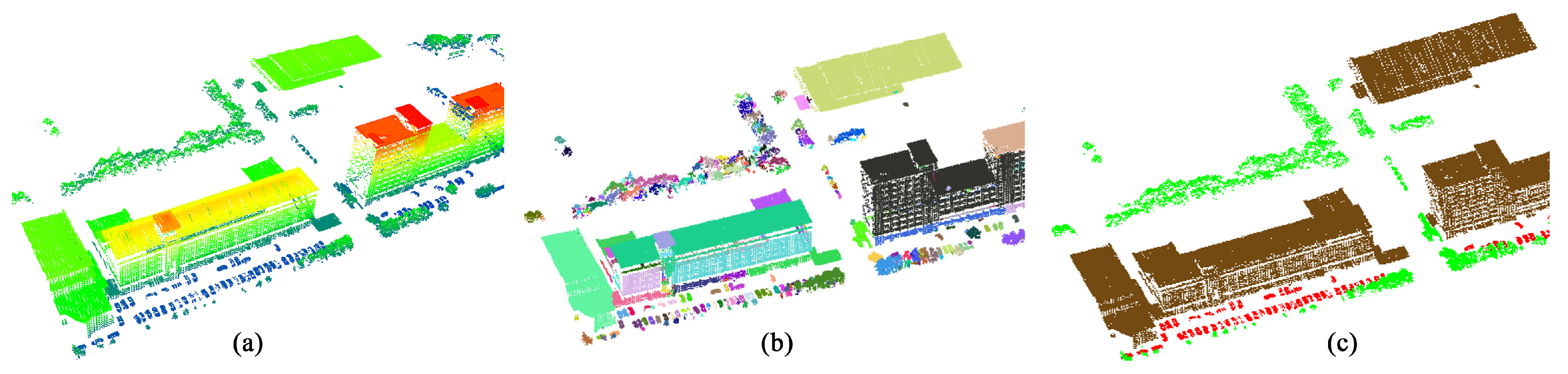
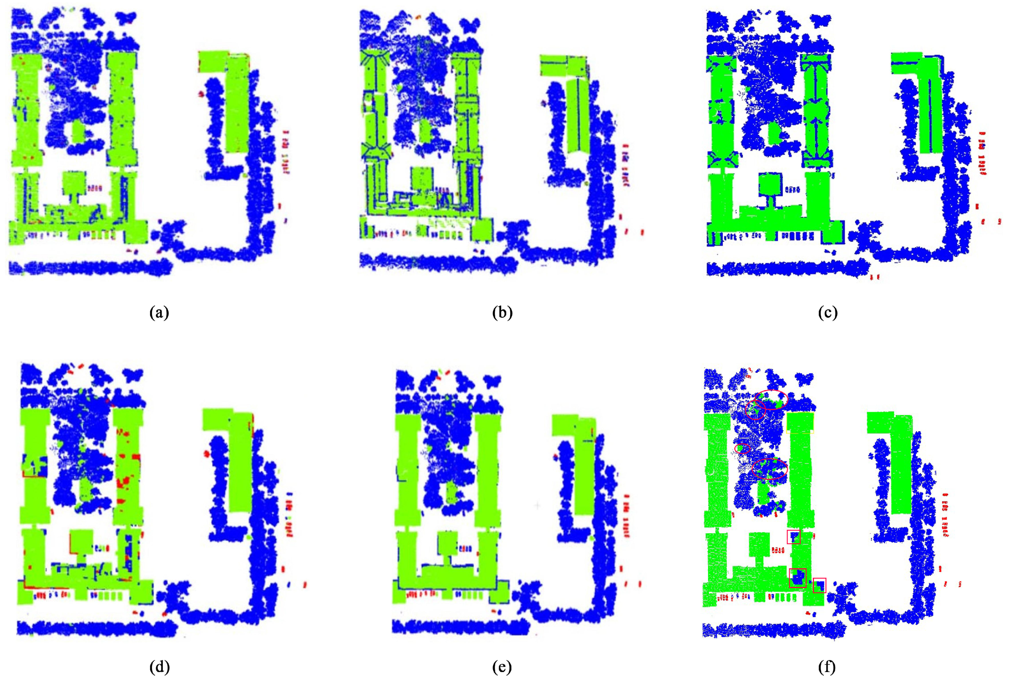
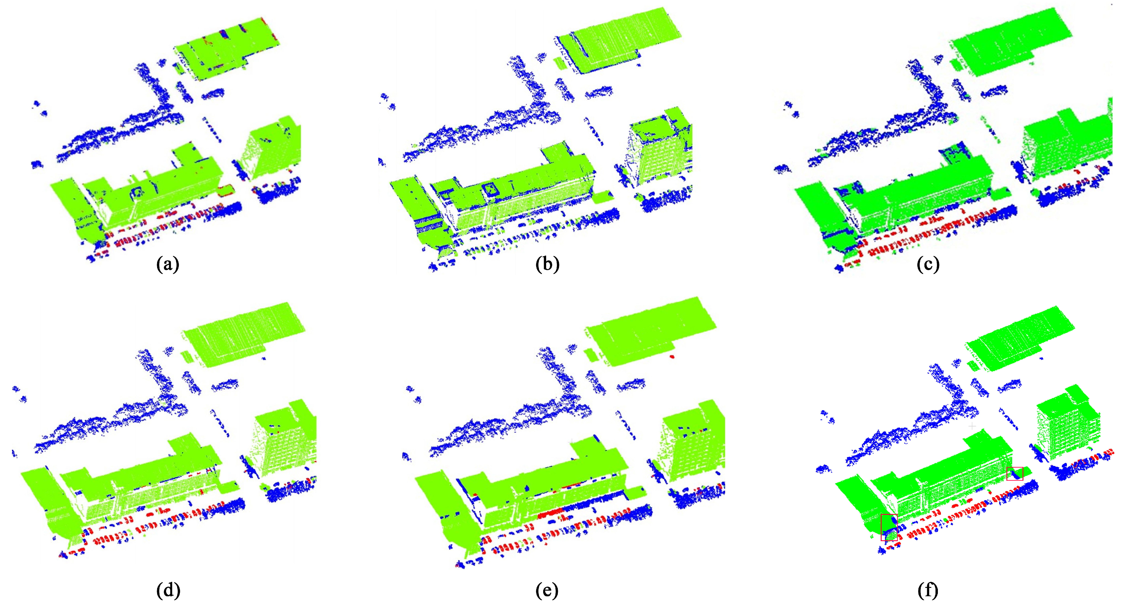
3.2. Comparisons
3.3. Effectiveness of CRF Model
3.4. Discussions
- (a)
- Self-adaptive Segmentation: In outdoor scenes, the objects have various shapes and sizes. The simple segmentation according to rigid number and the size of the clusters cannot adapt to various objects. In this case, the self-adaptive segmentation algorithm is required. The proposed workflow is adaptation-aware and is shown in two aspects: ➀ The coarse-grained clustering using the DBSCAN can identify any shapes of clusters according to the distribution of point clouds. The implementation cannot require the number of clusters and can easily find the noise and outliers. ➁ We propose probability density clustering algorithm to ensure topological maintenance between adjacent fined-grained clusters. The adaptive characteristics is represented by aggregating different number of fine-grained clusters into a high-level cluster, from which one-to-many relationships are included. That is the number of fine-grained clusters in a generated cluster is not fixed and is determined by the shapes and local properties of the objects. Self-adaptive segmentation ensures reasonableness of generated clusters at different levels.
- (b)
- Multilevel Clustering: The feature of cluster is more robust and stable compared to individual point clouds. Therefore, we propose three-level cluster generation strategy: the first level creates coarse-level clusters using DBSCAN algorithm. The second level clustering uses conventional k-means algorithm to over-segment the coarse-level clusters into a set of fine-grained clusters. The proposed probability density clustering algorithm works at the third level; it aggregates the fine-grained cluster set into a high-level scale, i.e., the third-level cluster set includes one-to-many relationships with the second-level clusters. Multilevel clustering can better explore the contextual information between the objects in outdoor scenes. Although there exists a multilevel cluster construction algorithm in [13], the size of generated clusters is linearly increased, causing no apparent feature discrepancy of the objects.
- (c)
- Higher-Order CRF Optimization: To optimize the point labeling using the proposed higher-order CRF model, we not only consider the adjacent clusters but a wider local area based on the neighborhood relationship between the clusters. More precisely, we design the higher-order potential and embed it into the CRF optimization. The higher-order potential can fully perceive the prior knowledge and contextual clues, thereby improving the accuracy of classification and recognition.
4. Conclusions
Author Contributions
Funding
Acknowledgments
Conflicts of Interest
References
- Yang, B.; Dong, Z. A shape-based segmentation method for mobile laser scanning point clouds. ISPRS J. Photogramm. Remote Sens. 2013, 81, 19–30. [Google Scholar] [CrossRef]
- Yang, B.; Dong, Z.; Zhao, G.; Dai, W. Hierarchical extraction of urban objects from mobile laser scanning data. ISPRS J. Photogramm. Remote Sens. 2015, 99, 45–57. [Google Scholar] [CrossRef]
- Landrieu, L.; Simonovsky, M. Large-scale point cloud semantic segmentation with superpoint graphs. In Proceedings of the IEEE Conference on Computer Vision and Pattern Recognition, Salt Lake City, UT, USA, 18–22 June 2018; pp. 4558–4567. [Google Scholar]
- Yang, B.; Dong, Z.; Liu, Y.; Liang, F.; Wang, Y. Computing multiple aggregation levels and contextual features for road facilities recognition using mobile laser scanning data. ISPRS J. Photogramm. Remote Sens. 2017, 126, 180–194. [Google Scholar] [CrossRef]
- Bircher, A.; Alexis, K.; Burri, M.; Oettershagen, P.; Omari, S.; Mantel, T.; Siegwart, R. Structural inspection path planning via iterative viewpoint resampling with application to aerial robotics. In Proceedings of the 2015 IEEE International Conference on Robotics and Automation (ICRA), Seattle, WA, USA, 25–30 May 2015; pp. 6423–6430. [Google Scholar]
- Gonzalez-Aguilera, D.; Crespo-Matellan, E.; Hernandez-Lopez, D.; Rodriguez-Gonzalvez, P. Automated urban analysis based on LiDAR-derived building models. IEEE Trans. Geosci. Remote Sens. 2013, 51, 1844–1851. [Google Scholar] [CrossRef]
- Li, Y.; Tong, G.; Du, X.; Yang, X.; Zhang, J.; Yang, L. A Single Point-Based Multilevel Features Fusion and Pyramid Neighborhood Optimization Method for ALS Point Cloud Classification. Appl. Sci. 2019, 9, 951. [Google Scholar] [CrossRef]
- Ni, H.; Lin, X.; Zhang, J. Classification of ALS point cloud with improved point cloud segmentation and random forests. Remote Sens. 2017, 9, 288. [Google Scholar] [CrossRef]
- Weinmann, M.; Jutzi, B.; Hinz, S.; Mallet, C. Semantic point cloud interpretation based on optimal neighborhoods, relevant features and efficient classifiers. ISPRS J. Photogramm. Remote Sens. 2015, 105, 286–304. [Google Scholar] [CrossRef]
- Mei, J.; Zhang, L.; Wang, Y.; Zhu, Z.; Ding, H. Joint Margin, Cograph, and Label Constraints for Semisupervised Scene Parsing From Point Clouds. IEEE Trans. Geosci. Remote Sens. 2018, 56, 3800–3813. [Google Scholar] [CrossRef]
- Li, Y.; Tong, G.; Li, X.; Zhang, L.; Peng, H. MVF-CNN: Fusion of Multilevel Features for Large-Scale Point Cloud Classification. IEEE Access 2019, 7, 46522–46537. [Google Scholar] [CrossRef]
- Zhang, Z.; Zhang, L.; Tan, Y.; Zhang, L.; Liu, F.; Zhong, R. Joint discriminative dictionary and classifier learning for ALS point cloud classification. IEEE Trans. Geosci. Remote Sens. 2018, 56, 524–538. [Google Scholar] [CrossRef]
- Xu, Z.; Zhang, Z.; Zhong, R.; Chen, D.; Sun, T.; Deng, X.; Li, Z.; Qin, C.Z. Content-Sensitive Multilevel Point Cluster Construction for ALS Point Cloud Classification. Remote Sens. 2019, 11, 342. [Google Scholar] [CrossRef]
- Jeong, J.; Lee, I. Classification of LIDAR Data for Generating a High-Precision Roadway Map. Int. Arch. Photogramm. Remote Sens. Spat. Inf. Sci. 2016, 3, 251–254. [Google Scholar] [CrossRef]
- Tóvári, D.; Pfeifer, N. Segmentation based robust interpolation-a new approach to laser data filtering. Int. Arch. Photogramm. Remote Sens. Spat. Inf. Sci. 2005, 36, 79–84. [Google Scholar]
- Papon, J.; Abramov, A.; Schoeler, M.; Worgotter, F. Voxel cloud connectivity segmentation-supervoxels for point clouds. In Proceedings of the IEEE Conference on Computer Vision and Pattern Recognition, Portland, OR, USA, 23–28 June 2013; pp. 2027–2034. [Google Scholar]
- Fischler, M.A.; Bolles, R.C. Random sample consensus: A paradigm for model fitting with applications to image analysis and automated cartography. Commun. ACM 1981, 24, 381–395. [Google Scholar] [CrossRef]
- Wang, Y.; Shi, H. A Segmentation Method for Point Cloud Based on Local Sample and Statistic Inference. In Geo-Informatics in Resource Management and Sustainable Ecosystem; Springer: Berlin, Germany, 2015; pp. 274–282. [Google Scholar]
- Ni, K.; Jin, H.; Dellaert, F. Groupsac: Efficient consensus in the presence of groupings. In Proceedings of the 2009 IEEE 12th International Conference on Computer Vision, Kyoto, Japan, 27 September–4 October 2009; pp. 2193–2200. [Google Scholar]
- Shahbazi, M.; Sohn, G.; Théau, J. Evolutionary optimization for robust epipolar-geometry estimation and outlier detection. Algorithms 2017, 10, 87. [Google Scholar] [CrossRef]
- Raguram, R.; Chum, O.; Pollefeys, M.; Matas, J.; Frahm, J.M. USAC: A universal framework for random sample consensus. IEEE Trans. Pattern Anal. Mach. Intell. 2013, 35, 2022–2038. [Google Scholar] [CrossRef]
- Awadallah, M.; Abbott, L.; Ghannam, S. Segmentation of sparse noisy point clouds using active contour models. In Proceedings of the 2014 IEEE International Conference on Image Processing (ICIP), Paris, France, 27–30 October 2014; pp. 6061–6065. [Google Scholar]
- MacQueen, J. Some methods for classification and analysis of multivariate observations. In Proceedings of the Fifth Berkeley Symposium on Mathematical Statistics and Probability, Oakland, CA, USA, 21 June–18 July 1967; Volume 1, pp. 281–297. [Google Scholar]
- Wu, Y.; Li, F.; Liu, F.; Cheng, L.; Guo, L. Point Cloud Segmentation Using Euclidean Cluster Extraction Algorithm With the Smoothness. Meas. Control Technol. 2016, 35, 36–38. [Google Scholar]
- Cheng, Y. Mean shift, mode seeking, and clustering. IEEE Trans. Pattern Anal. Mach. Intell. 1995, 17, 790–799. [Google Scholar] [CrossRef]
- Comaniciu, D.; Meer, P. Mean shift: A robust approach toward feature space analysis. IEEE Trans. Pattern Anal. Mach. Intell. 2002, 5, 603–619. [Google Scholar] [CrossRef]
- Mei, J.; Wang, Y.; Zhang, L.; Zhang, B.; Liu, S.; Zhu, P.; Ren, Y. PSASL: Pixel-Level and Superpixel-Level Aware Subspace Learning for Hyperspectral Image Classification. IEEE Trans. Geosci. Remote Sens. 2019. [Google Scholar] [CrossRef]
- Feng, C.; Taguchi, Y.; Kamat, V.R. Fast plane extraction in organized point clouds using agglomerative hierarchical clustering. In Proceedings of the 2014 IEEE International Conference on Robotics and Automation (ICRA), Hong Kong, China, 31 May–7 June 2014; pp. 6218–6225. [Google Scholar]
- Zhang, Z.; Zhang, L.; Tong, X.; Mathiopoulos, P.T.; Guo, B.; Huang, X.; Wang, Z.; Wang, Y. A multilevel point-cluster-based discriminative feature for ALS point cloud classification. IEEE Trans. Geosci. Remote Sens. 2016, 54, 3309–3321. [Google Scholar] [CrossRef]
- Xu, Y.; Yao, W.; Tuttas, S.; Hoegner, L.; Stilla, U. Unsupervised segmentation of point clouds from buildings using hierarchical clustering based on Gestalt principles. IEEE J. Sel. Top. Appl. Earth Observ. Remote Sens. 2018, 99, 1–17. [Google Scholar] [CrossRef]
- Ester, M.; Kriegel, H.P.; Sander, J.; Xu, X. A density-based algorithm for discovering clusters in large spatial databases with noise. Kdd 1996, 96, 226–231. [Google Scholar]
- Liu, P.; Zhou, D.; Wu, N. VDBSCAN: Varied density based spatial clustering of applications with noise. In Proceedings of the 2007 International Conference on Service Systems and Service Management, Chengdu, China, 9–11 June 2007; pp. 1–4. [Google Scholar]
- Li, M.; Sun, C. Refinement of LiDAR point clouds using a super voxel based approach. ISPRS J. Photogramm. Remote Sens. 2018, 143, 213–221. [Google Scholar] [CrossRef]
- Rusu, R.B.; Bradski, G.; Thibaux, R.; Hsu, J. Fast 3d recognition and pose using the viewpoint feature histogram. In Proceedings of the 2010 IEEE/RSJ International Conference on Intelligent Robots and Systems, Taipei, Taiwan, 18–22 October 2010; pp. 2155–2162. [Google Scholar]
- Aldoma, A.; Vincze, M.; Blodow, N.; Gossow, D.; Gedikli, S.; Rusu, R.B.; Bradski, G. CAD-model recognition and 6DOF pose estimation using 3D cues. In Proceedings of the 2011 IEEE International Conference on Computer Vision Workshops (ICCV Workshops), Barcelona, Spain, 6–13 November 2011; pp. 585–592. [Google Scholar]
- Lai, K.; Fox, D. Object recognition in 3D point clouds using web data and domain adaptation. Int. J. Robot. Res. 2010, 29, 1019–1037. [Google Scholar] [CrossRef]
- Chen, D.; Peethambaran, J.; Zhang, Z. A supervoxel-based vegetation classification via decomposition and modelling of full-waveform airborne laser scanning data. Int. J. Remote Sens. 2018, 39, 2937–2968. [Google Scholar] [CrossRef]
- Zhang, W.; Qi, J.; Wan, P.; Wang, H.; Xie, D.; Wang, X.; Yan, G. An easy-to-use airborne LiDAR data filtering method based on cloth simulation. Remote Sens. 2016, 8, 501. [Google Scholar] [CrossRef]
- Wang, Z.; Zhang, L.; Zhang, L.; Li, R.; Zheng, Y.; Zhu, Z. A Deep Neural Network With Spatial Pooling (DNNSP) for 3-D Point Cloud Classification. IEEE Trans. Geosci. Remote Sens. 2018, 56, 4594–4604. [Google Scholar] [CrossRef]
- Lafferty, J.; McCallum, A.; Pereira, F.C. Conditional random fields: Probabilistic models for segmenting and labeling sequence data. In Proceedings of the Eighteenth International Conference on Machine Learning, Williamstown, MA, USA, 28 June–1 July 2001; Volume 1, pp. 282–289. [Google Scholar]
- Kohli, P.; Kumar, M.P.; Torr, P.H. P3 & Beyond: Move Making Algorithms for Solving Higher Order Functions. IEEE Trans. Pattern Anal. Mach. Intell. 2009, 31, 1645–1656. [Google Scholar]
- Kohli, P.; Torr, P.H. Robust higher order potentials for enforcing label consistency. Int. J. Comput. Vis. 2009, 82, 302–324. [Google Scholar] [CrossRef]
- Vineet, V.; Warrell, J.; Torr, P.H. Filter-based mean-field inference for random fields with higher-order terms and product label-spaces. Int. J. Comput. Vis. 2014, 110, 290–307. [Google Scholar] [CrossRef]
- Fix, A.; Wang, C.; Zabih, R. A primal-dual algorithm for higher-order multilabel markov random fields. In Proceedings of the IEEE Conference on Computer Vision and Pattern Recognition, Columbus, OH, USA, 23–28 June 2014; pp. 1138–1145. [Google Scholar]
- Guo, B.; Huang, X.; Zhang, F.; Sohn, G. Classification of airborne laser scanning data using JointBoost. ISPRS J. Photogramm. Remote Sens. 2015, 100, 71–83. [Google Scholar] [CrossRef]
- Wang, Z.; Zhang, L.; Fang, T.; Mathiopoulos, P.T.; Tong, X.; Qu, H.; Xiao, Z.; Li, F.; Chen, D. A multiscale and hierarchical feature extraction method for terrestrial laser scanning point cloud classification. IEEE Trans. Geosci. Remote Sens. 2015, 53, 2409–2425. [Google Scholar] [CrossRef]
- Zhang, Z.; Zhang, L.; Tong, X.; Guo, B.; Zhang, L.; Xing, X. Discriminative-dictionary-learning-based multilevel point-cluster features for ALS point-cloud classification. IEEE Trans. Geosci. Remote Sens. 2016, 54, 7309–7322. [Google Scholar] [CrossRef]
- Zhang, Z. ALS Point Cloud Classification Based on Multilevel Point Cluster Features. Ph.D. Thesis, Beijing Normal University, Beijing, China, 2016. [Google Scholar]
- Xia, S.; Wang, R. Extraction of residential building instances in suburban areas from mobile LiDAR data. ISPRS J. Photogramm. Remote Sens. 2018, 144, 453–468. [Google Scholar] [CrossRef]
- Khoshelham, K.; Nardinocchi, C.; Frontoni, E.; Mancini, A.; Zingaretti, P. Performance evaluation of automated approaches to building detection in multi-source aerial data. ISPRS J. Photogramm. Remote Sens. 2010, 65, 123–133. [Google Scholar] [CrossRef] [Green Version]


| Training Data | Testing Data | |||||
|---|---|---|---|---|---|---|
| Tree | Building | Vehicle | Tree | Building | Vehicle | |
| Scene 1 | 68,802 | 37,128 | 5380 | 213,990 | 200,549 | 7816 |
| Scene 2 | 39,743 | 64,952 | 4584 | 73,207 | 156,186 | 7409 |
| Features | Description | |
|---|---|---|
| ++ | Sum of feature values | |
| Full variance | ||
| The entropy of feature values | ||
| Anisotropy property | ||
| Planarity property | ||
| Linear property | ||
| Scattered property | ||
| Horizontal property | ||
| - | Elevation characteristics | |
| - | Latitudinal sampling histogram |
| Methods | Basic Unit | Point Set Construction | Feature Expression | Optimization | Classifier |
|---|---|---|---|---|---|
| Method 1 | Individual point | None | Geometry, strength, and statistical characteristics | Region growth | JointBoost |
| Method 2 | Individual point | None | Spin Image feature and | None | AdaBoost |
| Method 3 | Individual point | None | Multiscale | Multiscale neighbor | SVM |
| Method 4 | Point set | Graph cut and linear transformation | LDA model based on Spin Image features and Fcov | None | AdaBoost |
| Method 5 | Point set | Graph cut and exponential transformation | DD-SCLDA model based on Spin Image feature and | Discriminating inheritance | AdaBoost |
| Our Method | Point set | Multilevel clustering | High-order CRF | SVM |
| Scene 1 | Methods | Tree (%) | Building (%) | Vehicle (%) | Accuracy (%) | -Score (%) | m(%) |
| Method 1 | 85.7/92.9 | 92.0/83.8 | 56.9/54.7 | 87.9 | 89.2/87.7/55.8 | 77.5 | |
| Method 2 | 89.7/98.1 | 97.9/89.1 | 65.2/46.6 | 92.9 | 93.7/93.3/54.4 | 80.5 | |
| Method 3 | 99.2/84.9 | 86.8/99.3 | 99.9/42.7 | 91.9 | 91.5/92.7/59.8 | 81.3 | |
| Method 4 | 94.8/93.8 | 93.5/92.3 | 41.2/66.7 | 92.6 | 94.3/92.9/50.9 | 79.4 | |
| Method 5 | 93.1/96.0 | 95.2/92.6 | 73.3/62.2 | 93.7 | 94.5/93.9/67.3 | 85.2 | |
| Our Method | 95.5/96.4 | 96.1/95.4 | 76.7/70.9 | 95.4 | 95.9/95.8/73.7 | 88.5 | |
| Scene 2 | Methods | Tree (%) | Building (%) | Vehicle (%) | Accuracy (%) | -Score (%) | m (%) |
| Method 1 | 73.9/91.2 | 93.6/88.2 | 29.5/25.4 | 87.2 | 81.6/90.8/27.3 | 66.6 | |
| Method 2 | 86.8/91.2 | 96.8/95.5 | 44.1/34.8 | 92.2 | 88.9/96.1/38.9 | 74.7 | |
| Method 3 | 83.2/92.9 | 98.5/92.8 | 62.6/65.7 | 92.0 | 95.6/87.8/64.1 | 82.5 | |
| Method 4 | 90.3/93.9 | 97.6/96.5 | 49.4/42.0 | 94.1 | 92.1/97.0/45.4 | 78.2 | |
| Method 5 | 94.7/94.5 | 98.1/97.7 | 53.9/60.5 | 95.5 | 94.6/97.9/57.0 | 83.2 | |
| Our Method | 92.3/94.5 | 98.2/97.8 | 71.5/62.8 | 95.2 | 93.4/98.0/66.9 | 86.1 |
| Scene 1 | Configurations | Tree (%) | Building (%) | Vehicle (%) | m (%) |
| Without CRF | 92.5 | 90.5 | 67.9 | 83.7 | |
| Low-level CRF | 92.7 | 93.6 | 68.9 | 85.1 | |
| High-level CRF | 95.9 | 95.8 | 73.7 | 88.5 | |
| Scene 2 | Configurations | Tree (%) | Building (%) | Vehicle (%) | m (%) |
| Without CRF | 85.9 | 94.7 | 61.1 | 80.6 | |
| Low-level CRF | 90.2 | 96.1 | 64.2 | 83.5 | |
| High-level CRF | 93.4 | 98.0 | 66.9 | 86.1 |
© 2019 by the authors. Licensee MDPI, Basel, Switzerland. This article is an open access article distributed under the terms and conditions of the Creative Commons Attribution (CC BY) license (http://creativecommons.org/licenses/by/4.0/).
Share and Cite
Li, Y.; Chen, D.; Du, X.; Xia, S.; Wang, Y.; Xu, S.; Yang, Q. Higher-Order Conditional Random Fields-Based 3D Semantic Labeling of Airborne Laser-Scanning Point Clouds. Remote Sens. 2019, 11, 1248. https://0-doi-org.brum.beds.ac.uk/10.3390/rs11101248
Li Y, Chen D, Du X, Xia S, Wang Y, Xu S, Yang Q. Higher-Order Conditional Random Fields-Based 3D Semantic Labeling of Airborne Laser-Scanning Point Clouds. Remote Sensing. 2019; 11(10):1248. https://0-doi-org.brum.beds.ac.uk/10.3390/rs11101248
Chicago/Turabian StyleLi, Yong, Dong Chen, Xiance Du, Shaobo Xia, Yuliang Wang, Sheng Xu, and Qiang Yang. 2019. "Higher-Order Conditional Random Fields-Based 3D Semantic Labeling of Airborne Laser-Scanning Point Clouds" Remote Sensing 11, no. 10: 1248. https://0-doi-org.brum.beds.ac.uk/10.3390/rs11101248