Article

Reconstruction of Ocean Color Data Using Machine Learning Techniques in Polar Regions: Focusing on Off Cape Hallett, Ross Sea

1
Department of Oceanography, Pusan National University, Geumjeong-Gu, Busan 46241, Korea
2
Korea Polar Research Institute, Incheon 21990, Korea
3
Underwater Survey Technology 21, Incheon 21999, Korea
*
Author to whom correspondence should be addressed.
Remote Sens. 2019, 11(11), 1366; https://0-doi-org.brum.beds.ac.uk/10.3390/rs11111366
Submission received: 1 May 2019 / Revised: 4 June 2019 / Accepted: 4 June 2019 / Published: 6 June 2019
(This article belongs to the Section Ocean Remote Sensing)

Abstract

:
The most problematic issue in the ocean color application is the presence of heavy clouds, especially in polar regions. For that reason, the demand for the ocean color application in polar regions is increased. As a way to overcome such issues, we conducted the reconstruction of the chlorophyll-a concentration (CHL) data using the machine learning-based models to raise the usability of CHL data. This analysis was first conducted on a regional scale and focused on the biologically-valued Cape Hallett, Ross Sea, Antarctica. Environmental factors and geographical information associated with phytoplankton dynamics were considered as predictors for the CHL reconstruction, which were obtained from cloud-free microwave and reanalysis data. As the machine learning models used in the present study, the ensemble-based models such as Random forest (RF) and Extremely randomized tree (ET) were selected with 10-fold cross-validation. As a result, both CHL reconstructions from the two models showed significant agreement with the standard satellite-derived CHL data. In addition, the reconstructed CHLs were close to the actual CHL value even where it was not observed by the satellites. However, there is a slight difference between the CHL reconstruction results from the RF and the ET, which is likely caused by the difference in the contribution of each predictor. In addition, we examined the variable importance for the CHL reconstruction quantitatively. As such, the sea surface and atmospheric temperature, and the photosynthetically available radiation have high contributions to the model developments. Mostly, geographic information appears to have a lower contribution relative to environmental predictors. Lastly, we estimated the partial dependences for the predictors for further study on the variable contribution and investigated the contributions to the CHL reconstruction with changes in the predictors.

Graphical Abstract

1. Introduction

Since the 1970s when satellite ocean color observations were possible, related research has been developing rapidly [1]. This observation has contributed to scientific advances [2] in coastal management, fisheries, and the detection of a harmful algae bloom. Besides, the societal benefits of ocean color observations include an increased ability to locate potential fishing zones and the ability to monitor water quality and fragile ecosystems [2,3,4,5]. Despite the widespread availability of ocean color observations, mapping of ocean color is spatiotemporally limited and challenged by inconsistent information due to cloud covers [6,7,8,9,10], particularly in polar regions [11,12]. The polar regions are usually covered by dense clouds throughout the year [12], and, thus, the valid range of satellite observations is narrow. As such, the many gaps in the ocean color data for polar regions limit the application of ocean color data to research in these regions [9]. As a result, the demand for continuous ocean color data on various spatial and temporal scales in the polar regions has increased.
To date, many researchers have attempted to fill the gaps of ocean color data contaminated by the presence of clouds. In particular, a conventional approach called the Data Interpolating Empirical Orthogonal Functions (DINEOF) is widely used for the reconstruction of ocean color data in various regions [13,14,15,16,17,18,19,20,21,22,23,24,25,26]. The DINEOF is purely based on data interpolation via iteration until the matrix converges. This EOF-based analysis can extract dominant spatial patterns from the time-series datasets through an iterative process [7]. Recently, new attempts to reconstruct the ocean color data using machine learning-based algorithms are intermittent [8,9,27]. Machine learning is one of the reliable and cost-effective approaches that could reconstruct the inevitable gaps in the ocean color data and is a predictive model. In particular, the approach is more flexible than conventional parametric models because of its ability to handle non-linear relationships and complex interactions, which often occur in ecological data [28,29,30]. Jouini et al. [9] attempted to recover significant gaps in satellite-derived chlorophyll concentration (CHL) data using Self Organizing Maps (SOM) classification (instance-based machine learning) in the western sector of the North Atlantic. They used the sea surface temperature (SST) and height (SSH) data as predictors for CHL estimation based on the assumption that a state of the ocean could be regionally defined by the SST, SSH, and CHL. Results show that the reconstruction of CHL data using SOM is robust when there is extended cloud cover at spatial scales larger than approximately 10 km. Jo et al. [10] introduced the neural network technique to derive CHL in the regions with numerous cloud-induced gaps. They used the SST, cloud, water vapor, precipitation, and winds as predictors. As such, the reconstructed CHL has a correlation coefficient of 0.98 and an error of 0.30 mg m−3, comparable to the observed CHL. Krasnopolsky et al. [27] also applied the neural network technique to recover the gaps in ocean color data on a global scale using the physical variables derived from the satellite measurements such as SST, SSH, and sea surface salinity (SSS) and Argo in-situ data. They noted that the application of the approach could provide an accurate, computationally cheap method for filling spatial and temporal gaps in satellite observation. Besides, Chen et al. [8] reconstructed CHL data through an ensemble-based approach (Random forest, RF) using wavelength-based predictors. They showed a significant improvement of ocean color gap recovery of more than 300% over the regions of the Yellow Sea and the East China Sea, and the estimated CHL has a quality similar to the standard satellite-derived CHL.
All the previous studies on the CHL reconstruction mentioned above have shown significant performances in their respective study areas. However, the DINEOF is based on data interpolation via iteration until the matrix converges and it might not work well if there are not enough CHL data in those regions due to the extended cloud coverage throughout the year [7,31]. This issue could serve to limit the approach proposed by Chen et al. [8] that is based on spectral and ocean color index data. For multivariate DINEOF [13], it might work using the cloud-free data representing environmental factors associated with phytoplankton biomass. However, it has not been applied to the polar region to date, and it is required to compare with the approach proposed in this study. In addition, as with the approaches proposed by Jouini et al. [9] and Krasnopolsky et al. [27], a couple of oceanographic predictors are insufficient to describe the spatiotemporal CHL patterns influenced by a complex interaction of various factors such as atmospheric (wind, light, and temperature) and biogeochemical macro- and micronutrients components, including oceanic physical components [32,33,34,35,36,37]. Since the dominant phytoplankton species and their response to the environmental factors vary by region, a deep understanding of the phytoplankton dynamics in a target region is essential. Therefore, all the factors that might impact the regional phytoplankton dynamics should be considered to reconstruct CHL data suitable for that region.
The satellite standard CHL is based on blue-green band ratios and color index approach, and these approaches are based on the spectral signals of phytoplankton biomass. However, for the polar region, the spectral data are quite limited due to dense clouds. To date and to the best of our knowledge, no approaches have been applied to reconstruct CHL data in polar regions. Therefore, we aimed to reconstruct CHL data without missing values based on microwave and reanalysis data, which was immune to clouds, using the machine learning-based model on a regional scale, near Cape Hallett, Ross Sea, Antarctica. As predictors for the model, we considered various factors that may affect the atmospheric and oceanic physical conditions (such as stratification, convective mixing, and heat transfer), and the indirect biogeochemical states (e.g., micronutrients). The reconstructed CHL was finally calculated at the equivalent spatial (4 km) and temporal (daily) resolutions as those of the standard CHL data. The reconstructed CHL data were first compared to the available standard CHL products (pixel by pixel) to evaluate how similar the reconstructed CHL is to the standard satellite-derived CHL. Besides, to identify how well the model reconstructs the CHL where the satellites could not observe, the reconstructed CHL was compared with the in-situ CHL. Lastly, we attempted to estimate the quantitative contribution of each input variable to identify which variables are primarily associated with the model development for CHL data reconstruction and to investigate how the CHL reconstruction response to each predictor alteration.

2. Study Sites

The model performance for the reconstruction of CHL was focused on off Cape Hallett in northern Victoria Land, Ross Sea (Figure 1). Cape Hallett is an essential region for the large populations of breeding penguins by supporting large swarms of krill [38,39]. Because the krill abundance is directly linked to primary production [40], the detailed studies on primary production using CHL data in this region are also essential for understanding the variability in the penguin population. Nonetheless, because the region has only a few clear-sky days throughout the year due to dense cloud covers (Figure 1), satellite-based CHL data are rarely available. In the austral winter season, all regions are mostly covered by clouds, and the satellite-derived data represent a few cloud-free days in December and January confined to specific regions, such as Terra Nova Bay and a part of southern Ross Sea [41]. In the remaining regions, relatively more clouds exist, and the presence of sea ice also limits the ocean color observation considerably. Nonetheless, since the region includes the primary foraging areas of the penguins that mainly inhabit Cape Hallett (refer to Lyver et al. [42]), consistent monitoring and analysis of the regional primary production using complete and accurate CHL data are highly desirable.

3. Materials

3.1. Satellite and Reanalysis Data

Satellite and reanalysis data from 1998/1999 to 2017/2018 in summertime were used as the predictor data to estimate the un-gapped CHL using machine learning techniques. All data were used as the training and test datasets to develop the models for CHL reconstruction. Detailed information on the predictor variables and target data (only CHL) used in the present study is given in Table 1.

3.1.1. Sea Surface Temperature

SST data were from the Optimal Interpolation Sea Surface Temperature (OISST) database (https://www.ncdc.noaa.gov/oisst) [43]. These data were produced by combining in-situ observation, sea-ice model, and satellite observation conducted by the Advanced Very High-Resolution Radiometer and Advanced Microwave Scanning Radiometer at the National Center for Environmental Prediction. The OISST is recorded daily at a 25 km resolution. This product has been produced and archived since 1982.

3.1.2. Sea Ice Concentration

Sea ice concentration data were obtained from the European Organization for the Exploitation of Meteorological Satellites (EUMETSAT) Ocean and Sea Ice Satellite Application Facility (OSI SAF) (http://www.osi-saf.org) [44]. The data were reanalyzed using a hybrid algorithm, which is a combination of the Bootstrap algorithm in the frequency mode and the Bristol algorithm. Data are available on a 12.5 km Equal-Area Scalable Earth grid as well as a polar stereographic grid. The accuracy of sea ice concentration is on the order of 5% [45].

3.1.3. Atmospheric Components

ERA-interim reanalysis data obtained from the European Centre for Medium-Range Weather Forecasts (ECMWF) were used for the atmospheric variables, including 10-m zonal (U10) and meridional (V10) winds, 2-m air temperature (T2M), and photosynthetically active radiation (PAR) (https://www.ecmwf.int/) [46]. The reanalysis data incorporate observations from in-situ measurements, balloons, radiosondes, dropsondes, aircraft, and satellites [47]. It was provided at 6-hourly (U10, V10, and T2M) and 12-hourly (PAR) time intervals at the four main synoptic times 0000, 0600, 1200 and 1800 UTC. We averaged the data to produce a daily product, and the spatial resolution of the data was provided at 4 km, consistent with the resolution of the CHL data. Wind measurements in the ECMWF are highly accurate in the Ross Sea [48,49,50].

3.1.4. Geographical Information

The geographical data (latitude and longitude) were obtained from the CHL dataset. Besides, the General Bathymetric Chart of the Ocean (GEBCO) with 30 arc-second resolution was used to obtain information on the ocean floor depth (https://www.gebco.net/) [51]. This digital bathymetry was generated by combining ship depth soundings with the interpolation between the sounding points being guided by satellite gravity data [52].

3.1.5. Chlorophyll Concentration

The CHL data used as the target data in the present analysis were obtained from the European Space Agency’s GlobColour project (http://hermes.acri.fr/) [53]. They are the merged data from multiple sensors (such as Sea-viewing Wide Field-of-view Sensor, Moderate Resolution Imaging Spectroradiometer-Aqua, ad Medium Resolution Imaging Spectrometer) with the weighted averaging method (used in this study) during the time that multiple sensors can be used. Since it is essential to have many training data for machine learning, such CHL data based on the multiple sensors are suitable for this study. Besides, the merged data have been validated, and the full validation report states that the data are in good agreement overall (http://www.globcolour.info/validation/index.html) [53]. Ultimately, the daily merged CHL data at 4 km spatial resolution were used in the present study. The accuracy of satellite-derived CHL in the Ross Sea is a level of ±65% compared to in-situ measurements [41,54].

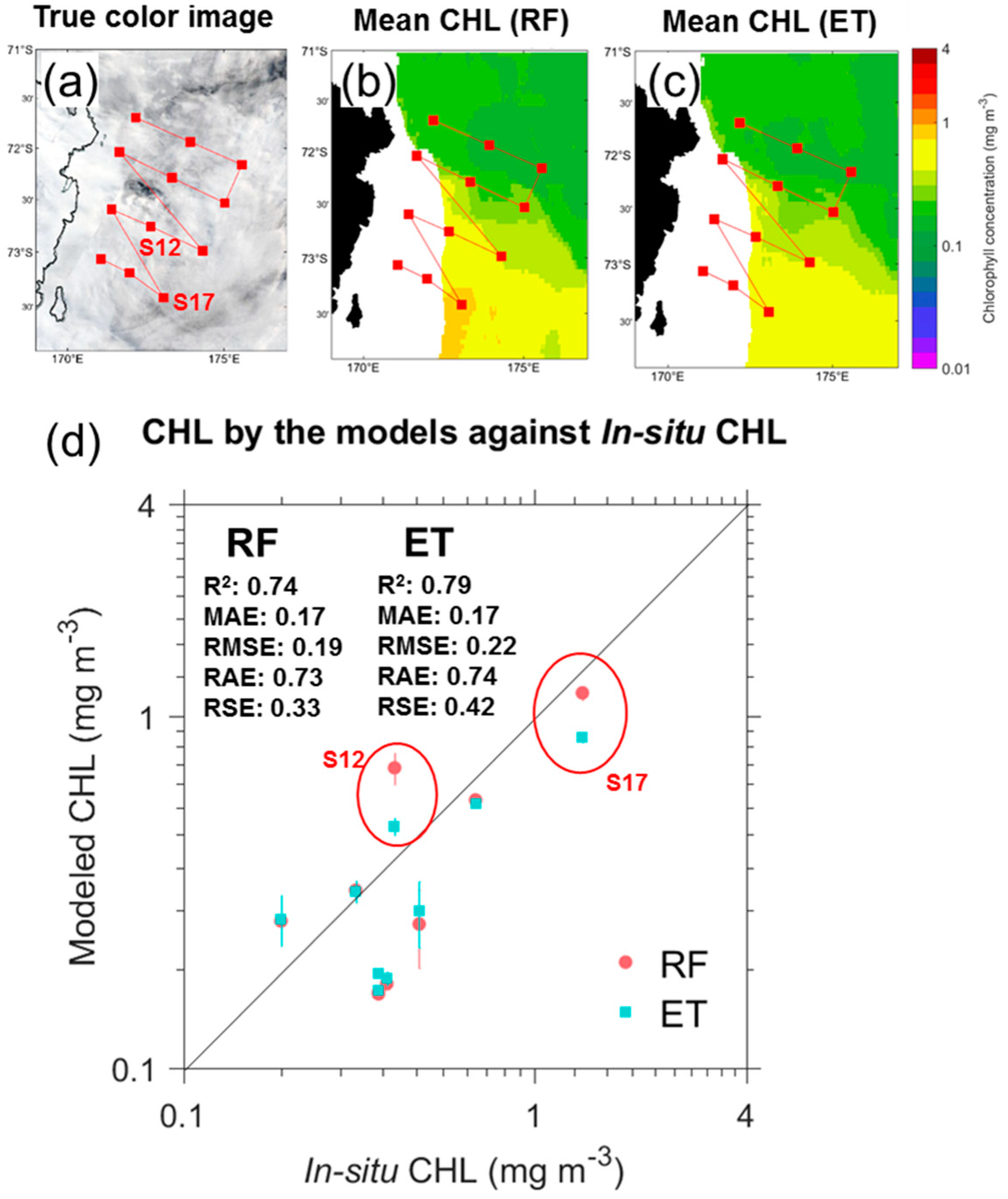
3.2. In-Situ Chlorophyll Concentration

In-situ CHL measurements were used to verify the reconstructed CHL data by the machine learning models. The field survey was conducted onboard the Korean Research vessel IBR/V Araon off Cape Hallett from 25 February to 1 March 2018 (ANA08C) (Figure 1b and Table 2). CHL samples (0.3 or 0.5 L) were collected from six different depths (100%, 50%, 30%, 12%, 5%, and 1% light depths) at 12 stations (S02–S19) using 10 L Niskin bottles. Then, water samples were filtered through 25 mm GF/F filter papers (Whatman, 0.7 μm pore) to measure the total CHL. Filtered samples were extracted in 90% acetone in the dark for 24 h [55]. Then, CHL fluorescence with 95% accuracy was measured onboard using a Trilogy laboratory fluorometer (Turner, UK) [55]. Among the CHL from the six different depths, we only used the surface CHL to ensure that the models yielded CHL that is close to the real CHL in the regions with missing values.

4. Methods

This study was limited to the austral spring and summer seasons (October to March) because CHL data are mostly lacking due to the sea ice cover and clouds during the austral winter. The workflow for the reconstruction of CHL during that seasons is shown in Figure 2. First, the data for the model development and application were preprocessed, including the SST, SIC, U10, V10, T2M, PAR, DEP, LON, and LAT and the CHL data as target classes (the “class” refers to the output category of the data and represents the CHL values in this study). The justification for the predictor selection is described in Section 3.1.2. The preprocessed data were randomly separated into training and test sets to be used for the model design and performance (1998/1999−2017/2018 seasons, October to March). The most critical work in this study was to select the appropriate model based on the given datasets and to determine the optimized model parameters (called the hyperparameters) in the selected model to derive the most accurate output. We used the 10-fold cross-validation method to assess the accuracy of the different models [30]. Once models with good performance were selected, the grid-search approach was used to identify hyperparameters in the model. This approach is a method to find the best model performance by changing parameters at regular intervals. Finally, we set up the selected models using the determined hyperparameters, and inputted all available predictor datasets into the model without any split. As such, we could obtain the modeled CHL during the entire period. For the evaluation of CHL data reconstruction, we compared between the modeled CHL approximates the standard satellite-derived CHL. Besides, it was compared with in-situ data to identify how similarly the model can reconstruct CHL to real CHL in the region where there are no standard CHL data.

4.1. Predictor Selection

The selection of inadequate predictors could generate noises in the class estimation by over-learning an unimportant predictor. To avoid this noise, a deep understanding of the factors that influence the class is needed. We, therefore, referred to previous studies [11,33,34,35,36,37,56,57,58,59,60,61,62,63,64,65,66] on the growth/limitation of phytoplankton that determine CHL in this region and finally selected the predictors.
In the western Ross Sea including Cape Hallett, distinct phytoplankton blooms are recurrent from year to year during austral spring and summer, especially around the Terra Nova Bay [11,63]. The phytoplankton growth results from the combinations of many factors such as sea ice, temperature, wind, nutrients, and light [37,64,65,66]. In these regions, each factor is not solely involved in a specific process. For instance, the light availability, the primary limiting factor for the phytoplankton growth [33,34,35,36,37], could be controlled by not only the change in solar radiation itself, but also the extent of stratification resulting from a vertical mixing by winds [56,57,66] or ice melting by a heat flux between atmosphere and ocean.
Another limiting factor, micronutrients such as iron [37,58,59], is mainly supplied to the surface layer due to the vigorous convective mixing during austral winter [66], but new supply can occur due to the melting of sea ice in austral spring and summer [60]. In addition, the process of iron-enriched water mass entering the continental shelf from outside the shelf may be another source of new iron supply in shallow areas [61]. The ice patterns in the western Ross Sea are mainly determined by the thermodynamic (melting) or dynamic (drift) factors, in which the temperature, wind, and light interact [62]. In addition, the inflow from out of the continental shelf could accelerate the ice melting by increasing the sensible heat flux [61]. Since all factors involved in determining the CHL features in this region are complicatedly connected, we tried to use all the available primary data to consider all these effects as fully as possible. Finally, the SIC reflecting the ice pattern, the SST and the T2M that include thermal factors such as heat flux, the wind (U10 and V10) that can cause a convective mixing and an ice drift, the PAR for light availability, and the geographical information (latitude, longitude, and bathymetry) were finally selected as predictor variables for the CHL reconstruction.

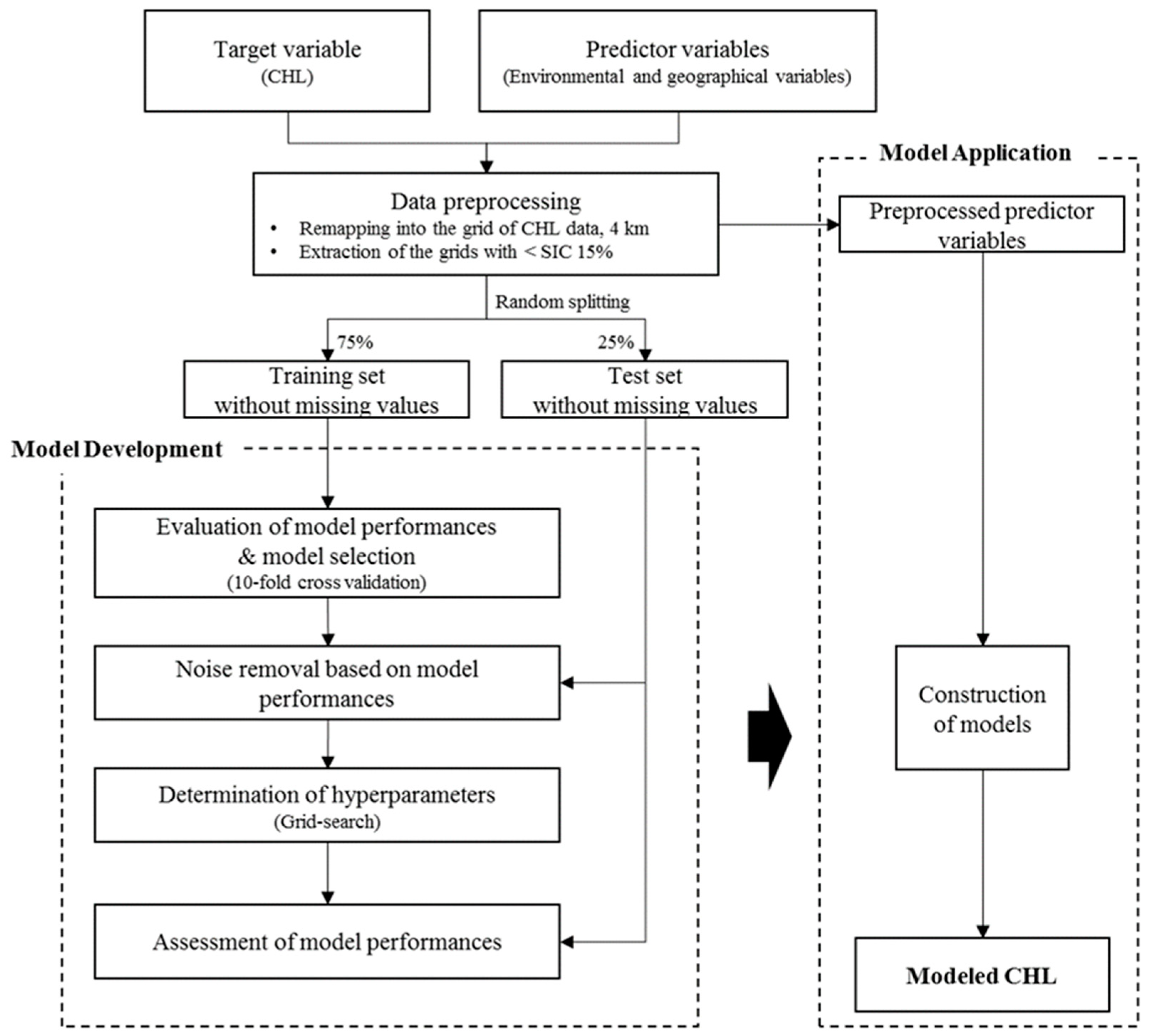
4.2. Data Preprocessing

Although each predictor dataset has its own spatial resolution (Table 1), all predictors used in the machine learning model for the CHL reconstruction were remapped at the 4 km spatial resolution of CHL data using the simple bilinear interpolation method [67]. Since all remapped predictor datasets are based on microwave and reanalysis data with almost no missing values, they enable a full CHL reconstruction except for land areas. However, as this region has amounts of sea ice, CHL produced in pixels with dense SIC might be doubtful. Then, the machine learning models were applied in only the pixels that represent less than 15% SIC as the marginal ice edge (NSIDC, 2019). This was based on the assumption that regions with SIC of less than 15% are open water areas.
In the machine learning model, class imbalance and noise are essential considerations when performing a machine learning model [68]. They generally occur when the training data are not evenly distributed across all classes and concentrated on a certain few classes. If such issues exist, the overall accuracy for the model performance might be diminished because rare classes are not adequately trained [69,70]. The class imbalance issue is common in many real-world applications [71], including ocean color data. Besides, ocean color data occasionally have some noise error due to the atmospheric states such as aerosols and clouds, or digitization error. Therefore, abnormally high CHL values often appear in a few pixels. If these values are not removed, this could cause a model failure for construction of CHL. To overcome the issues, we determined the range of class that can show the best performance of the models. This approach is likely to improve the overall accuracy of the model performance by resolving the class imbalance issue to some extent and removing the noise simultaneously. Therefore, we analyzed the class distribution used in the model development process, and the detailed results are described in Section 3.2.

4.3. Machine Learning Models

We first tested which model is most appropriate for the CHL reconstruction. Several machine learning-based models were selected in the test, such as instance-based (e.g., k-Nearest Neighbor), regression-based (e.g., linear and logistic regressions), single decision tree, and ensemble-based models consisting of boosting (e.g., gradient boosting machine) and Bootstrap Aggregating (bagging) such as RF [72] and Extremely Randomized Tree (ET) [73]. The test was performed for both training and test datasets using the 10-fold cross-validation [74]. Except for the ensemble-based model (accuracy > 0.8), other models showed poor performances for both training and test sets (accuracy < 0.7). Thus, we covered only the two ensemble-based models (RF and ET) that were excellent in performance evaluation in the present study. The details on the evaluation between the two models are described in Section 3.1.
Both models selected as the most suitable models for the reconstruction of CHL data in this region are based on the bagging techniques in the ensemble-based models. The bagging technique is a sort of ensemble technique and can improve the stability and accuracy of model performance [75]. Besides, it reduces variance in iterative results of the model and allows avoiding overfitting, causing little difference in performance between training and test datasets. In particular, the bagging techniques might be appropriate for the data containing noise [68]. The RF is a well-known machine learning technique for classification and regression of data. It consists of an ensemble of various single decision trees for subset data, which are resampled randomly from the training data [76]. The ET is an ensemble of a certain number of randomized trees that adds more randomization to the RF [73,77]. Both RF and ET are computationally efficient and capable of handling very high-dimensional features [75,77]. However, the ET has a shorter training time than the RF in that it takes a simple approach to select thresholds on the node. Moreover, it reduces variance, when compared with the RF, due to its increased randomization [73,77].

4.4. Model Development

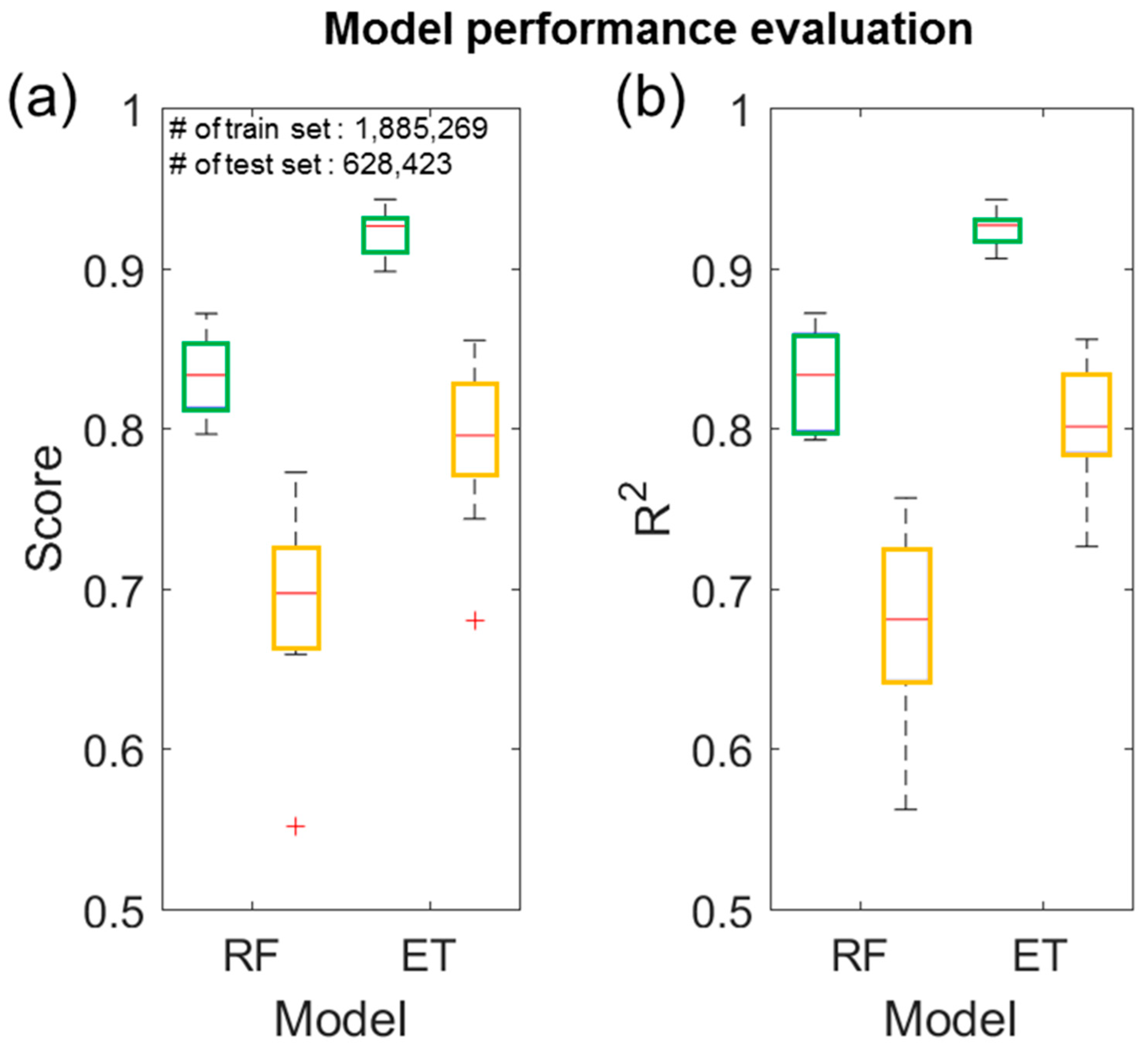
4.4.1. Model Comparison

To compare model performances, the performances of two leading models (RF and ET) were evaluated using the 10-fold cross-validation analysis (Figure 3). It was applied to both training and test sets, and score and coefficient of determination (R2) were used as metrics for this evaluation. The score shown here is a measure of accuracy, and is calculated as the number of correct predictions made as a ratio of all predictions and standardized (that is, the accuracy is in the range of 0–1).
The median score (red bar) of the RF and ET model performances for training data are 0.84 and 0.93, respectively (Figure 3a). The range of the RF model scores (0.82–0.85) has a wider interquartile range (distance between the top and bottom sides of the box) than that the ET model scores (0.92–0.93). In general, the interquartile range could be considered a more robust measure to assess the stability of the data. Thus, the ET model with narrow range is likely to be more stable in terms of performance than the RF model. The median scores of the RF and ET models for test dataset (RF: 0.70; ET: 0.80) are about 83% and 86% of those in the models for the training dataset, respectively. The stabilities of both model performances are similar, but they have unstable properties compared to the results of training data from the outlier generation and wider interquartile range (RF: 0.66–0.73, ET: 0.77–0.83). This feature is similar in R2 (Figure 3b). The median R2 on the RF model performance for the training data is 0.83, and that of the ET model performance is 0.93. The model performances for the test data are 0.68 and 0.80, respectively. The stability properties are similar to that of the score (RF: 0.80–0.86 for training data and 0.64–0.72 for test data, ET: 0.92–0.93 for training data and 0.78–0.83 for test data).
In these results, the significant differences between the metrics for the training and test data imply a sort of overfitting to the training data. Besides, the results for the test data are significantly unstable compared to those for the training data due to the small number of data as one-third of the training data. However, the current process was simply performed without the determination of the hyperparameter, thus the relative comparison between the two models is more meaningful.
In summary, the ET model shows better performance than the RF model and is more stable for the training data. Since the class balance of training and test sets are similar (not shown), the performance accuracy of both the RF and ET models is less sensitive to the changes in the number of data to be trained alone, and the ET model is likely to be somewhat more sensitive than the RF model in terms of model stability.

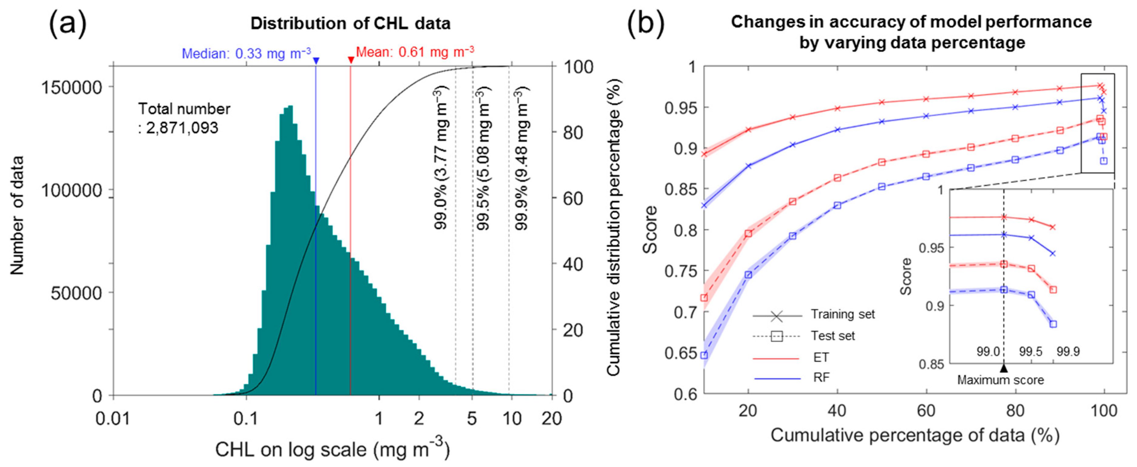
4.4.2. Class Imbalance and Noise on CHL Data

Class imbalance and noise are essential considerations when performing a machine learning model [68]. Class imbalance occurs when the training data are not evenly distributed across all classes and concentrated on a certain few classes. If such imbalance exists, the overall accuracy for the model performance might be diminished because rare classes are not adequately trained [69,70]. Class imbalance is a common problem in nature [71], especially in the CHL data the issue is significant due to seasonal characteristics of phytoplankton dynamics and regional ecological difference. Therefore, even if this issue cannot be eliminated, some mitigation is needed. Although the bagging techniques exert good performances in handling the class imbalance in noisy data [68], we sorted the CHL data using an appropriate CHL threshold values to remove noise and mitigate the class imbalance issue for more accurate CHL reconstruction.
The distribution of CHL data trained in this study shows such imbalance clearly (Figure 4a). The total of 2,871,093 CHL values are unevenly distributed around the mean of 0.61 mg m−3 and a median of 0.33 mg m−3, and the highest accumulation occurs at 0.21 mg m−3. In this distribution, the high CHL values appearing on the rightmost few of the distribution may contain some noises, not actual CHL values. Therefore, we tried to remove the noise included in these data based on a specific threshold. For the determination of the specific threshold, we tried to identify the changes in the model performances by varying the class range (Figure 4b). In general, as the cumulative percentage of CHL range in the data increases, both models progressively improve performances and show high stability over iterative model results. However, since the maximum scores of the model performances record about 0.96 in the RF model and 0.97 in the ET model for the training set at the 99.0% data range (0.94 in the RF model and 0.91 in the ET model for the test set), after that, the model performance begins to decline. This suggests that data quality is critical as well as data quantity. Consequently, based on the accuracy and stability of the scores, we determined the final threshold for the 99.0% cumulative percentage of data in this study. That is, the CHL training data were confined to the range of 0–3.77 mg m−3 CHL (Figure 4a) and data with CHL values above the range were considered as noise or cause of class imbalance issue and excluded in this analysis.

4.4.3. Determination of Hyperparameters

All evaluations of model performance mentioned above were conducted using the generalized RF and ET models without any tuning of the model parameters. It was, therefore, necessary to find the hyperparameters to derive the best accuracy of the two selected models to obtain the best reconstruction of the CHL. To determine the hyperparameters of both RF and ET models, the 10-fold grid-search method was applied. The commonly critical parameters in these two models are “number of trees (Ntree)” and “number of features (Mtry)” [76,78]. Here, “feature” indicates the predictor variable. We applied the method by changing the Ntree from 1 to 1000 with 100 intervals. Since a total of features used in this study is 9, the method was applied on a grid of one unit from 2 to 9. The reason the interval of grid-search for Ntree was set to 100 is to ensure the efficiency of the model performance time. Besides, it was roughly decided based on the argument of the previous study that the difference in the results of the model with hyperparameter control is not distinct [79]. Finally, the hyperparameters were estimated as Ntree = 700 and Mtry = 7 in the RF model and Ntree = 700 and Mtry = 9 in the ET model. The performances of the RF and ET models using the hyperparameters were significantly improved, as shown in Table 3, compared with the results in the model evaluation described in Section 3.1 (Figure 3). The evaluation metrics associated with the model performances for training and test datasets mostly indicate that the models performed well against the given data, and the ET model shows a better performance than the RF model for the reconstruction of the CHL data, numerically.

5. Results

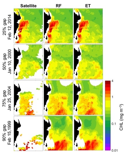
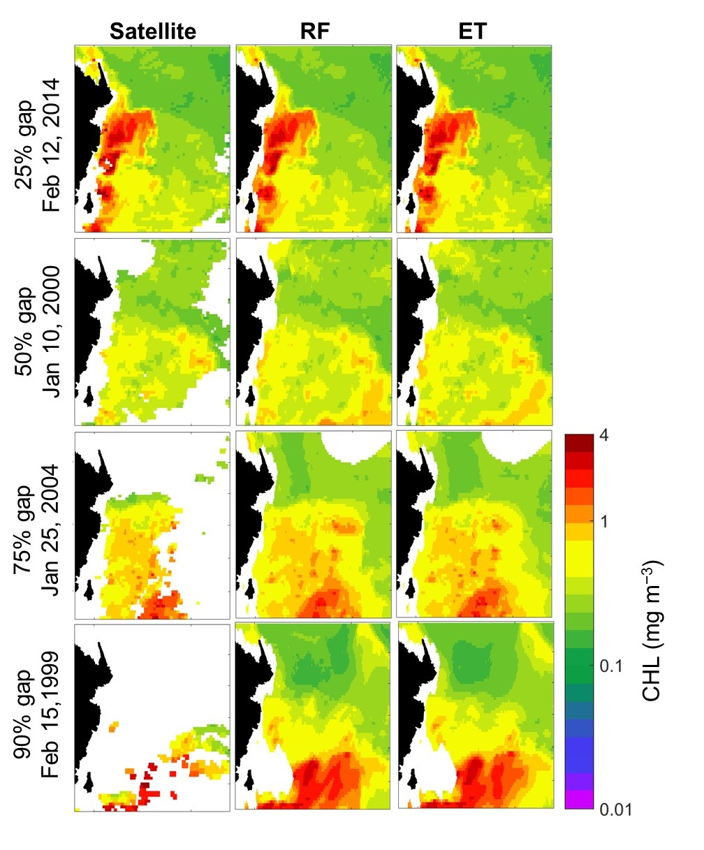
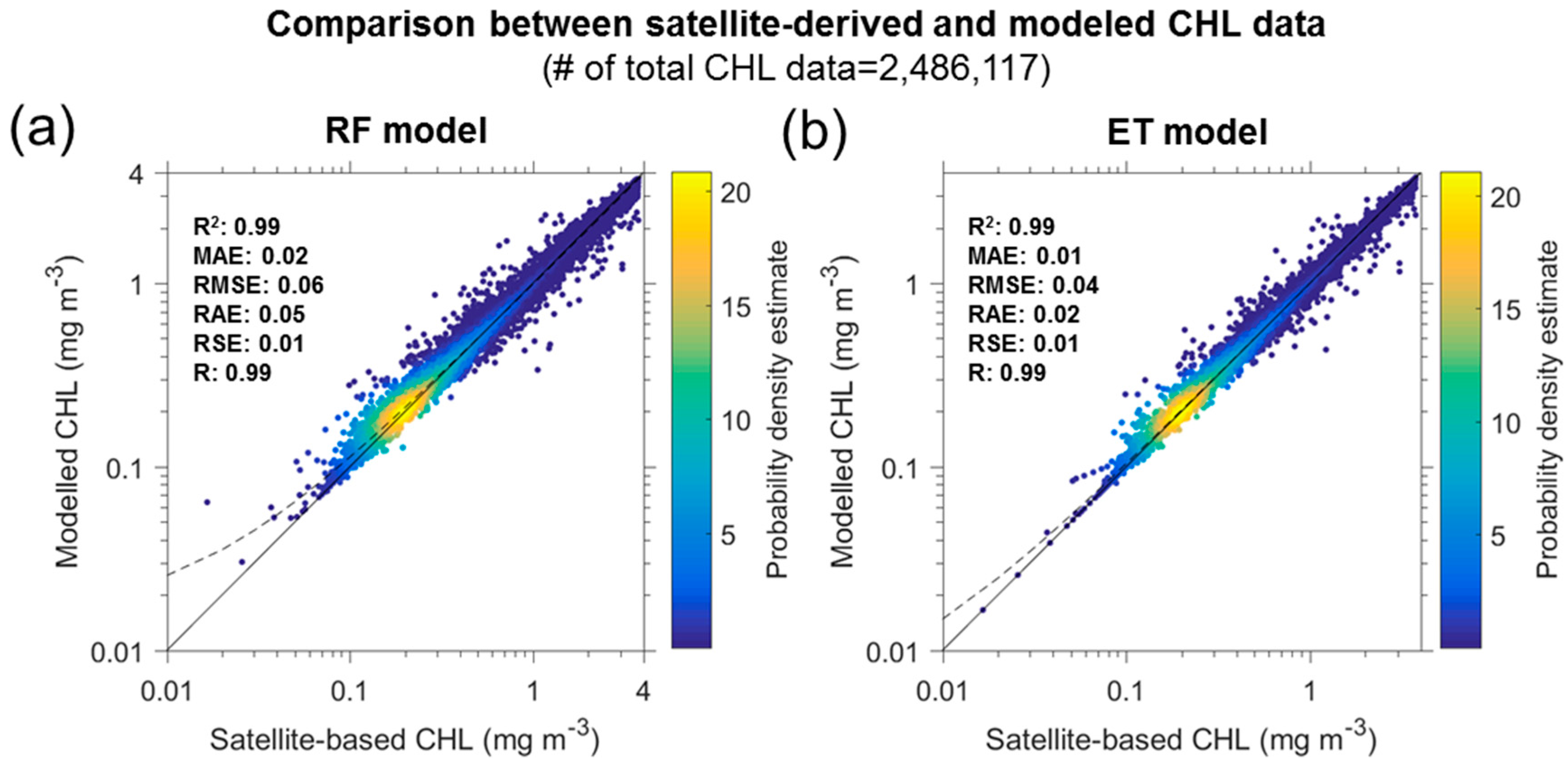
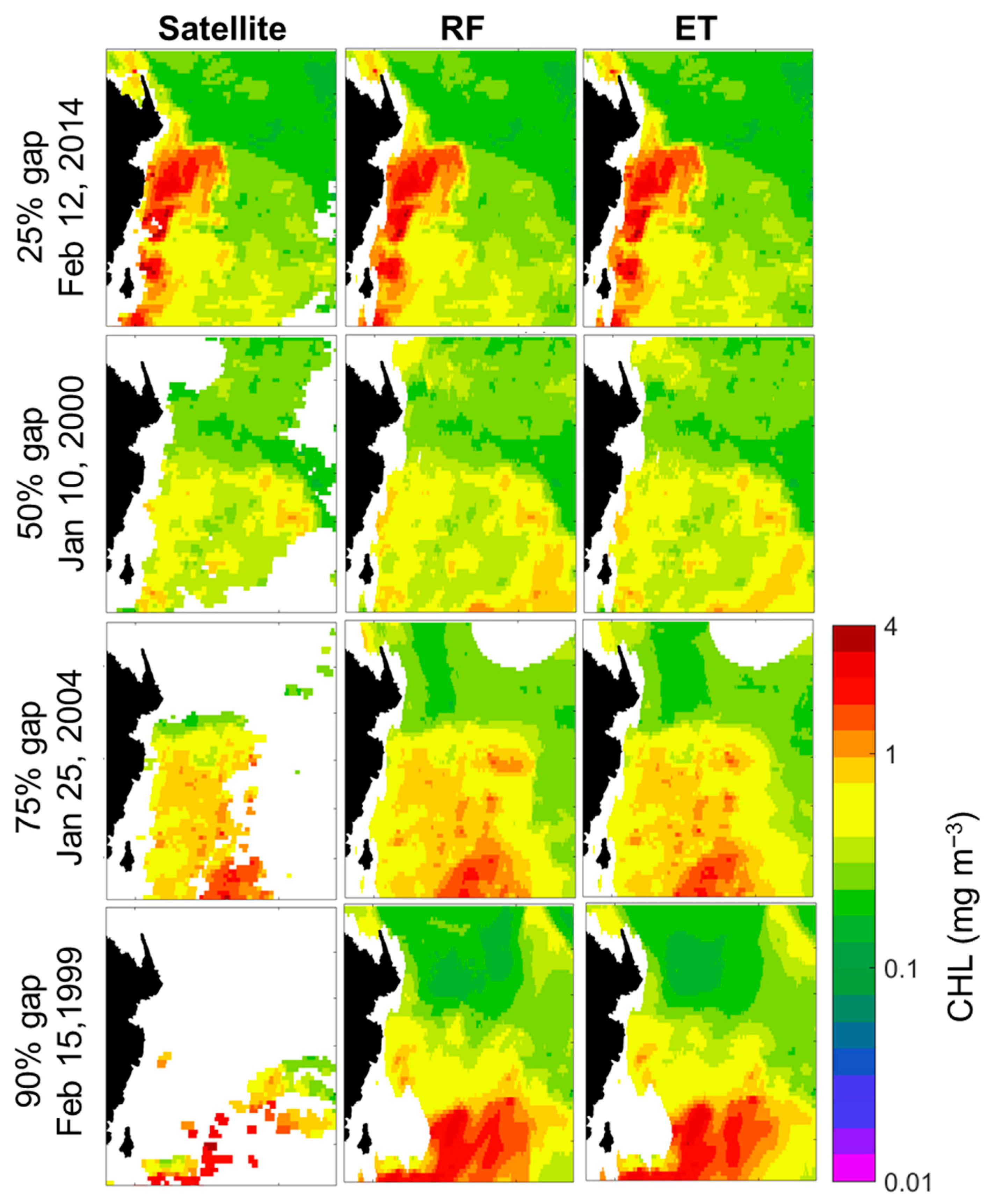
5.1. Reconstruction of CHL Data

The preprocessed predictor variable was input to the developed models without any split into training and test sets, and the CHL was modeled and compared with the standard satellite data. The scatterplot between the observed CHL and modeled CHL by the RF, and ET models are shown in Figure 5. The comparison was conducted at the available pixels (2,486,117) in the standard satellite data. The probability density estimates are concentrated on the range of 0.15–0.30 mg m−3, corresponding the original distribution of CHL data (Figure 4a). However, it is clear that the consistency of the modeled CHL for most satellite-based CHL is quite high. The RF model slightly overestimates at the CHL values lower than 0.3 mg m−3 because a small number of data for training. In addition, values less than 0.1 mg m−3 do not make much sense because data are scarcely rare, and we exclude them from this interpretation.
Further, to verify the ability of spatial reconstruction of the two machine learning techniques, we compared the spatial distributions of the satellite-derived and modeled CHL, as shown in Figure 6. As examples, the images were selected based on the gap proportions of 25% (12 February 2014), 50% (10 January 2000), 75% (25 January 2004), and 90% (15 February 1999). CHL on 12 February 2014 has a 25% gap proportion, which was the fewest gaps during the entire study period. The other proportions were set arbitrarily. The satellite-based image with gaps of about 25% for CHL distribution has significant numbers of valid pixels, but there are few missing values in the coastal regions and some regions of the southeastern part of the domain. Except for missing values in the coastal regions induced by the high SIC (>15%), the pixels in the southeastern part are reconstructed well by the RF and ET models. The spatial CHL patterns reconstructed by both models are quite similar. In particular, these results show that the modeled CHL is well reconstructed without substantial modification compared to the remotely observed CHL. As such, the distribution of high CHL along the coast represents at the identical CHL level as the observed CHL. The satellite image with 50% gaps has many missing values over the coastal regions and parts of the east of this domain but reconstructed by both models. The patch with relatively high CHL of ~1 mg m−3 that was not observed was reconstructed by both models in the southeast of the domain, but this spatial feature shows slight differences between the RF and ET models. More details are needed as to whether the distinct features in the modeled CHL data, which were unobserved by satellites, are based on real CHL values. Unfortunately, there are no comparable in-situ data in this region for that date, as discussed below, to compare with our in-situ data. On days with more gaps (75% and 90%), the reconstruction by both models seems reasonable. In particular, the satellite-derived image with 90% gaps has a few valid pixels confined to the south of this domain. Even the rare pixels show that there is a bloom with ~4 mg m−3 CHL, but they do not provide the exact spatial feature. Such a spatial feature could be confirmed through the reconstructed CHL distribution. In addition, the CHL distribution is completely reconstructed in the north of this domain.
Overall, the results of the CHL reconstruction by the two ensemble-based machine learning models show a good agreement with the standard satellite data and the spatial reconstruction was performed smoothly. In addition, this approach has reconstructed about 646% of the satellite-based data. However, we found that the CHL reconstructed in certain regions with large gaps on standard CHL data are occasionally not consistent between the two model results. For this discrepancy, to find which model is close to a real CHL, a directly observed CHL is required. Fortunately, the reconstructed CHL data for the period of our in-situ observations have some differences in the spatial features, and we tried to describe which model produces a CHL value similar to the real CHL value on a day with many gaps (Figure 7). From 26 February to 1 March 2018 (four days), the study area was covered by heavy clouds, and the valid pixels were rare throughout the days (Figure 7a). Except for the region with dense ice concentration, the remaining regions were reconstructed by the machine learning models (Figure 7b,c). The mean distributions of reconstructed CHL by both models for four days are mostly consistent, but not in some regions. In particular, around station S17, the reconstructed CHL by the RF model (1.16 ± 0.06 mg m−3) is higher than that by the ET model (0.87 ± 0.03 mg m−3) and closer to the real CHL (1.37 mg m−3) (Figure 7d). In addition, also around S12, there is a discrepancy between the two models that the CHL of the RF model (0.71 ± 0.08 mg m−3) is larger than that of the ET (0.49 ± 0.03 mg m−3). However, there is no significant difference in the reconstructed CHLs by both models in S12. Only on 28 February 2018, when field observation was performed at S12, the reconstructed CHL by the RF model is temporarily high in that region. This is likely to be due to the relatively low RF stability compared to the ET as previously suggested.

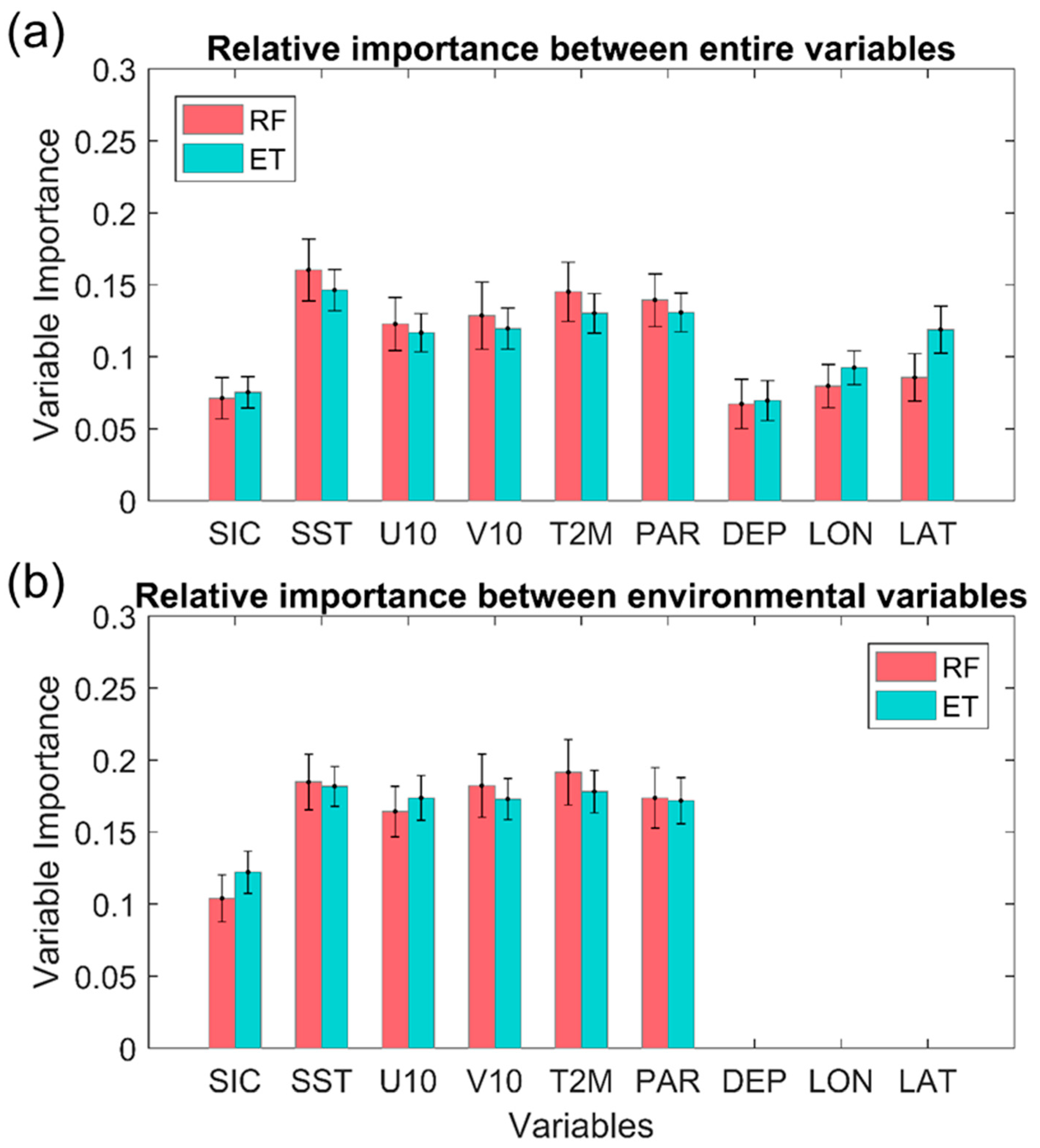
5.2. Contribution of Predictor Variables

The machine learning model quantitatively suggests the relative contribution of the predictor variables in the model development process (Figure 8a). The predictor variable with the highest contribution to the RF model is the SST at 16.0 ± 2.2% (mean ± standard deviation), followed by the T2M (14.5 ± 2.1%), PAR (13.9 ± 1.8), V10 (12.9 ± 2.3%), U10 (12.3 ± 1.8%), LAT (8.6 ± 1.7%), LON (8.0 ± 1.5%), SIC (7.1 ± 1.4%), and DEP (6.7 ± 1.7%). In the CHL reconstruction by the ET model, the SST showed the largest contribution (14.6 ± 1.4%), followed by PAR (13.1 ± 1.4%), T2M (13.0 ± 1.4%), V10 (12.0 ± 1.4%), LAT (11.9 ± 1.6%), U10 (11.7 ± 1.3%), LON (9.2 ± 1.2%), SIC (7.5 ± 1.1%) and DEP (7.0 ± 1.4%). The ranks of the predictor variables in both models are not entirely consistent, but the SST and T2M associated with thermal effects and the PAR have shown a significant contribution in those models, and the effects on the wind components are also not negligible. In general, the contribution of geographic information to the model is rather low. Unless this geographic information is considered, the contributions of other variables increase significantly (Figure 8b), but the overall model performances are reduced to 95% of the ET model performance for training data and 82% for test data (not shown). The RF model performance using only environmental datasets is reduced to 95% and 72% for training and test sets, respectively, compared to the performance using all predictors. This reduction in the performances for those datasets indicates that the geographical variables are also important to develop the machine learning model for the reconstruction of CHL data without gaps.
In addition, we estimated a partial dependence for each predictor to examine the effect of the predictors on the reconstructed CHL (Figure 9). To estimate the partial dependence on the CHL reconstruction, the other predictors except for the targeted predictor were fixed to their mean values during the entire study period. The experiment was carried out while varying the targeted predictor variable from the minimum value to the maximum value observed during the study period. The mean values of the individual predictor variable are SIC = 3.16%, SST = −0.57 °C, U10 = 1.22 m s−1, V10 = 2.28 m s−1, T2M = 271.76 K, PAR = 357,225 J m−2, DEP = 857.57 m, LON = 173.84° E, and LAT = 72.65° S. In both models, the partial dependences for each predictor are similar, but the dependence of both models for the SIC (Figure 9a) and the U10 (Figure 9c) are different. The partial dependence in the RF model for the SIC from 0% to 15% tends to increase with the growth in the SIC after the mean value of SIC (3.16%), while the ET model shows a negative relationship. For SST (Figure 9b), the partial dependences are constant in both models from the minimum to the mean value of the SST, and it shows a positive relation that the contribution to CHL increases with increasing SST. The U10 contributes to the CHL reconstruction at a similar level between the two models when blowing to the west (Figure 9c). The enhanced east wind component induces the CHL increases in the RF model, whereas the ET result is not significantly dependent on the U10. The V10 shows a distinct pattern, showing a decrease and a sharp increase before and after the mean V10, respectively (Figure 9d). Although the V10 does not show the highest contribution (Figure 9a), it appears to contribute more dramatically to the reconstructed CHL increase at higher wind speeds as well as the SST. The partial dependence for the T2M shows the lowest contribution in the mean T2M value (Figure 9e). Below the 271.76 K (≈−1.39 °C), the CHL is mainly constant. However, the CHL increases rapidly as the T2M increases above its mean value. The contribution of the PAR is insignificant until the mean PAR value, and then its contribution begins to increase after the mean PAR value (Figure 9f). However, such an increase is until the PAR reaches ~495,000 J m−2 and remains constant after that. The DEP shows unique peaks at ~500 m in both models (Figure 9g). In particular, it has a constant contribution of ~0.4 mg m−3 when the DEP reaches more than 500 m. At a depth of ~500 m, the contribution reaches its peak and then stable again. The result for the LON variable shows that the contribution to the CHL decreases gradually toward the east. In particular, in the west of 170°E, its contribution is constant, but it decreases sharply toward the east. In addition, it tends to have a constant contribution again to the east of 175°E. Lastly, the contribution of the LAT is increased to the south of the 72.6°S and shows a constant contribution to the north.

6. Discussion and Conclusions

The most problematic issue in utilizing ocean color observation is the existence of heavy clouds [10]. For the issue, the effort of reconstructing CHL data using the observed output from other sensors has been conducted by many researchers [8,9,10,19,27,80,81]. However, to date, no studies have been conducted in the polar regions, and it is expected that there will be difficulties in the construction of CHL in these regions by previous approaches. Thus, for the CHL reconstruction off Cape Hallett, we tried to reconstruct CHL using the machine learning techniques based on the cloud-free microwave and reanalysis datasets.
For the CHL reconstruction, the primary process performed in the present study could be largely divided into model development and application (Figure 2). In the process of model development, we selected the ensemble-based models (RF and ET) using the 10-fold cross-validation that are robust to the CHL reconstruction. As a result, both models showed the highest performances for the given data. However, this reconstruction has the limitation of reconstructing only the CHL values within the CHL range of 0–3.77 mg m−3. We removed the CHL data above 3.77 mg m−3 based on the data range with the best model performance score (Figure 4) to eliminate noise and to relieve class imbalance issue on CHL data. Although 99% of the CHL data observed in this region is distributed below 3.77 mg m−3 (Figure 4a), all values above 3.77 mg m−3 may not be true noise. Nonetheless, we used such a threshold for the primary purpose of reconstructing more accurate CHL within a given range than a larger range of CHL. In the future, to prevent loss of real CHL values and to solve the class imbalance, it is necessary to apply appropriate methods such as under- and over-sampling based on the high understanding of the characteristics of the target data [71,82,83].
The models developed based on the previous processes were consequently applied for the CHL construction off Cape Hallett. Both reconstructed CHL data from the developed RF and ET models showed significant agreements with the standard satellite-derived CHL data (Figure 5). Besides, regardless of the number of gaps, the spatial CHL reconstruction was carried out smoothly (Figure 6). However, there are occasionally the differences in the CHL reconstructions between the two models where no satellite was observed. The superiority can be inferred based on the higher performance of the ET model compared to the RF model in previous model evaluations (Figure 3 and Figure 5, and Table 3), but rather the reconstructed CHL of the RF model has the value closer to the real CHL than that of the ET model (Figure 7). Therefore, at the moment, it is quite challenging to determine which of the two models correctly reconstructed the CHL. However, regardless of the superiority between both models, we believe that CHL reconstructions were properly carried out with regard to the somewhat higher agreement with satellite and field observations.
In the variable importance results, the environmental variables (except SIC) play an essential role in model development (Figure 8). Although geographical information has a relatively low contribution, they are indispensable for accurate CHL reconstruction. In general, sea ice is a significant factor to drive the phytoplankton dynamics associated with light availability [37,84] and micronutrient supply [11,85,86]. Nonetheless, the contribution of SIC is relatively low (Figure 8; RF: 7.1 ± 1.4%, ET: 7.5 ± 1.1%), and the CHL reconstructions in both models respond differently to changes in SIC (Figure 9a). We first assumed that open water has less than 15% SIC and excluded the regions with more than 15% SIC in the present study. Thus, strictly speaking, the contribution of the SIC may not contribute significantly to the CHL reconstruction in the regions with 0–15% SICs because these areas can be equally considered as open water.
The little differences between RF and ET (refer to Figure 6 and Figure 7) might result from the differences in the partial dependence for the U10, T2M, and PAR. Where the U10 and the PAR are larger than their mean values, the CHL of the RF model is overestimated compared to that of the ET model, and the RF can be overestimated even where the T2M is low. These characteristics are related to the substantial differences in the CHL distributions from both models in the southeastern part of the domain on 10 January 2000 (Figure 6), and in the reconstructed CHL values by both models at S12 and S17 (Figure 7). Besides, the partial dependence for the SIC also shows a significant difference between the two models (Figure 9a). However, the SIC condition within the range of 0–15% do not contribute significantly to the reconstruction because they can be treated equally as open water as described above. In practice, since the partial dependence for the SIC varied within only the CHL range of 0.1 mg m−3 (y-axis in Figure 9a), the contribution of the SIC to model development is relatively small compared to other predictors.
The results in the present analysis show that the machine learning models could successfully reconstruct the CHL based on the nine environmental forcings and geographical information regardless of the heavy cloud cover off Cape Hallett. However, despite such robustness, there remains some margin for improvements. Because of the complex interactions that exist between physical and biological processes in phytoplankton bloom dynamics [87,88], it is limited to determine the characteristics of blooms with only a few factors. In particular, this study attempted to reconstruct the CHL using only the satellite-derived and reanalysis data confined to the ocean surface or above. Even though surface ocean features are somewhat related to subsurface properties, it is not easy to fully consider the factors and processes below the ocean surface that are hardly observed by satellites alone. In addition, the climate is consistently changing, and the climate-induced environmental changes affect the ecosystem through fluctuations in water stability, nutrients and light [89]. Since these changes could directly affect phytoplankton organisms, the contribution of each factor can change over time. In this approach, the predictability of the machine learning-based model can be highly sensitive to the selection of predictor data. Therefore, a deep understanding of CHL dynamics and consistent monitoring are required, and building model input parameters based on these understanding and monitoring is a crucial process.
The models in the present study are regionally developed, and for other regional application, regional parameterization is required. In particular, note that the decision of the domain can cause a severe imbalance in the distribution of the target class. The phytoplankton bloom, which has high CHL, appears to be limited to a specific region and has some spatial variability. If the configured domain contains the marginal parts of a blooming area, high CHL may appear intermittently in some sector within the domain affected by the boundary effect of the bloom. As such, the number of data that can be trained for high CHL values is inadequate and then degrade the accuracy of the regional model. To solve this imbalance problem, it is possible to apply some techniques such as under- and over-sampling methods appropriately according to the characteristics of the data [71,82,83], or to prevent such problems by using the proper domain in advance. In addition, because of the different species of phytoplankton that are locally responsible for bloom and the factors that affect the phytoplankton growth/limitation, a thorough preliminary investigation on the biological properties in the target region must be accompanied. In general, since the data acquisition at the proper resolution is critical to investigate the phytoplankton variability in the Ross Sea [90], it is expected that this approach will enable the long-term accumulation of CHL data with high spatial and temporal resolutions by minimizing many missing values of ocean color observations in polar regions. Furthermore, sampling stations in the Ross Sea are separated by tens of kilometers due to the high cost of vessel operation and inaccessibility [90]. For that reason, the CHL patterns have been generally inferred from only spatially sparse observations. Therefore, the estimation of more accurate spatial CHL patterns might be possible by combining the reconstructed CHL data presented in this study and in-situ data using a specific assimilation technique such as optimal interpolation method.
Although there is still room for improvement, this study was carried out to maximize the availability of the ocean data in the regions restricted by clouds and showed the effective CHL reconstruction and that this approach could successfully reconstruct the CHL in a regional scale. It interpolated only the gaps without any modification of the standard CHL values and the spatial continuity between the standard and reconstructed CHL pattern is also reasonable. In the future, we will identify applications in larger areas and will make various attempts to effectively reconstruct broader ranges of CHL. In addition, a sensitivity test of uncertainty of predictors will be performed to obtain more accurate reconstructed CHL. Through these processes, we expect to increase the usability of ocean color data, which are one of the basic data in polar research.

Author Contributions

Conceptualization, J.P. and Y.-H.J.; methodology, J.P. and B.-K.K.; validation, N.J. and S.H.L.; formal analysis, J.P. and D.B.; investigation, J.P. and D.B.; resources, J.-H.K., N.J. and S.H.L.; data curation, J.P.; writing—original draft preparation, J.P.; writing—review and editing, Y.-H.J. and S.H.L.; visualization, J.P.; supervision, H.-c.K. and Y.-H.J.; project administration, J.-H.K.; and funding acquisition, H.-c.K. and J.-H.K.

Funding

This research was supported by the “Ecosystem Structure and Function of Marine Protected Area (MPA) in Antarctica” project (PM18060), funded by the Ministry of Oceans and Fisheries (20170336), Korea, and by the National Research Foundation of Korea (NRF) grant funded by the Korea government (MSIP) (NRF-2018R1A2B2006555).

Conflicts of Interest

The authors declare no conflict of interest.

References

  1. O’Reilly, J.E.; Maritorena, S.; Mitchell, B.G.; Siegel, D.A.; Carder, K.L.; Garver, S.A.; Kahru, M.; McClain, C. Ocean color chlorophyll algorithms for SeaWiFS. J. Geophys. Res. Ocean. 1998, 103, 24937–24953. [Google Scholar] [CrossRef] [Green Version]
  2. Blondeau-Patissier, D.; Gower, J.F.R.; Dekker, A.G.; Phinn, S.R.; Brando, V.E. A review of ocean color remote sensing methods and statistical techniques for the detection, mapping and analysis of phytoplankton blooms in coastal and open oceans. Prog. Oceanogr. 2014, 123, 23–144. [Google Scholar] [CrossRef]
  3. Klemas, V. Remote Sensing Techniques for Studying Coastal Ecosystems: An Overview. J. Coast. Res. 2011, 27, 2–17. [Google Scholar] [CrossRef]
  4. Wilson, C. The rocky road from research to operations for satellite ocean-colour data in fishery management. ICES J. Mar. Sci. 2011, 68, 677–686. [Google Scholar] [CrossRef]
  5. Shen, L.; Xu, H.; Guo, X. Satellite remote sensing of harmful algal blooms (HABs) and a potential synthesized framework. Sensors (Switzerland) 2012, 12, 7778–7803. [Google Scholar] [CrossRef]
  6. Nechad, B.; Alvera-Azcaràte, A.; Ruddick, K.; Greenwood, N. Reconstruction of MODIS total suspended matter time series maps by DINEOF and validation with autonomous platform data. Ocean Dyn. 2011, 61, 1205–1214. [Google Scholar] [CrossRef] [Green Version]
  7. Liu, X.; Wang, M. Filling the Gaps of Missing Data in the Merged VIIRS SNPP/NOAA-20 Ocean Color Product Using the DINEOF Method. Remote Sens. 2019, 11, 178. [Google Scholar] [CrossRef]
  8. Chen, S.; Hu, C.; Barnes, B.B.; Xie, Y.; Lin, G.; Qiu, Z. Improving ocean color data coverage through machine learning. Remote Sens. Environ. 2019, 222, 286–302. [Google Scholar] [CrossRef]
  9. Jouini, M.; Lévy, M.; Crépon, M.; Thiria, S. Reconstruction of satellite chlorophyll images under heavy cloud coverage using a neural classification method. Remote Sens. Environ. 2013, 131, 232–246. [Google Scholar] [CrossRef]
  10. Jo, Y.; Kim, D.; Kim, H. Chlorophyll Concentration Derived from Microwave Remote Sensing Measurements USING Artificial Neural Network Algorithm. J. Mar. Sci 2018, 26, 102–110. [Google Scholar] [CrossRef]
  11. Arrigo, K.R.; Van Dijken, G.L. Annual changes in sea-ice, chlorophyll a, and primary production in the Ross Sea, Antarctica. Deep. Res. Part II Top. Stud. Oceanogr. 2004, 51, 117–138. [Google Scholar] [CrossRef]
  12. Marrari, M.; Hu, C.; Daly, K. Validation of SeaWiFS chlorophyll a concentrations in the Southern Ocean: A revisit. Remote Sens. Environ. 2006, 105, 367–375. [Google Scholar] [CrossRef]
  13. Alvera-Azcárate, A.; Barth, A.; Beckers, J.M.; Weisberg, R.H. Multivariate reconstruction of missing data in sea surface temperature, chlorophyll, and wind satellite fields. J. Geophys. Res. Ocean. 2007, 112. [Google Scholar] [CrossRef] [Green Version]
  14. Alvera-Azcárate, A.; Barth, A.; Sirjacobs, D.; Beckers, J.M. Enhancing temporal correlations in EOF expansions for the reconstruction of missing data using DINEOF. Ocean Sci. 2009, 5, 475–485. [Google Scholar] [CrossRef] [Green Version]
  15. Ruddick, K.; Lacroix, G.; Alvera-Azcárate, A.; Park, Y.; Nechad, B.; Sirjacobs, D.; Barth, A.; Beckers, J.-M. Cloud filling of ocean colour and sea surface temperature remote sensing products over the Southern North Sea by the Data Interpolating Empirical Orthogonal Functions methodology. J. Sea Res. 2010, 65, 114–130. [Google Scholar] [CrossRef]
  16. Volpe, G.; Nardelli, B.B.; Cipollini, P.; Santoleri, R.; Robinson, I.S. Seasonal to interannual phytoplankton response to physical processes in the Mediterranean Sea from satellite observations. Remote Sens. Environ. 2012, 117, 223–235. [Google Scholar] [CrossRef]
  17. Wang, Y.; Liu, D. Reconstruction of satellite chlorophyll-a data using a modified DINEOF method: A case study in the Bohai and Yellow seas, China. Int. J. Remote Sens. 2014, 35, 204–217. [Google Scholar] [CrossRef]
  18. Zhao, Y.; He, R. Cloud-free sea surface temperature and colour reconstruction for the gulf of mexico: 2003–2009. Remote Sens. Lett. 2012, 3, 697–706. [Google Scholar] [CrossRef]
  19. Alvera-Azcárate, A.; Vanhellemont, Q.; Ruddick, K.; Barth, A.; Beckers, J.M. Analysis of high frequency geostationary ocean colour data using DINEOF. Estuar. Coast. Shelf Sci. 2015, 159, 28–36. [Google Scholar] [CrossRef] [Green Version]
  20. Dreano, D.; Mallick, B.; Hoteit, I. Filtering remotely sensed chlorophyll concentrations in the Red Sea using a space-time covariance model and a Kalman filter. Spat. Stat. 2015, 13, 1–20. [Google Scholar] [CrossRef]
  21. Hilborn, A.; Costa, M. Applications of DINEOF to Satellite-Derived Chlorophyll-a from a Productive Coastal Region. Remote Sens. 2018, 10, 1449. [Google Scholar] [CrossRef]
  22. Jayaram, C.; Priyadarshi, N.; Pavan Kumar, J.; Udaya Bhaskar, T.V.S.; Raju, D.; Kochuparampil, A.J. Analysis of gap-free chlorophyll-a data from MODIS in Arabian Sea, reconstructed using DINEOF. Int. J. Remote Sens. 2018, 39, 7506–7522. [Google Scholar] [CrossRef]
  23. Liu, M.; Liu, X.; Ma, A.; Li, T.; Du, Z. Spatio-temporal stability and abnormality of chlorophyll-a in the northern south china sea during 2002-2012 from MODIS images using wavelet analysis. Cont. Shelf Res. 2014, 75, 15–27. [Google Scholar] [CrossRef]
  24. Liu, X.; Wang, M. Analysis of ocean diurnal variations from the Korean Geostationary Ocean Color Imager measurements using the DINEOF method. Estuar. Coast. Shelf Sci. 2016, 180, 230–241. [Google Scholar] [CrossRef]
  25. Liu, X.; Wang, M. Gap filling of missing data for VIIRS global ocean color products using the DINEOF Method. IEEE Trans. Geosci. Remote Sens. 2018, 56, 4464–4476. [Google Scholar] [CrossRef]
  26. Miles, T.N.; He, R. Temporal and spatial variability of Chl-a and SST on the South Atlantic Bight: Revisiting with cloud-free reconstructions of MODIS satellite imagery. Cont. Shelf Res. 2010, 30, 1951–1962. [Google Scholar] [CrossRef]
  27. Krasnopolsky, V.; Nadiga, S.; Mehra, A.; Bayler, E.; Behringer, D. Neural networks technique for filling gaps in satellite measurements: Application to ocean color observations. Comput. Intell. Neurosci. 2016, 2016. [Google Scholar] [CrossRef] [PubMed]
  28. Guisan, A.; Zimmermann, N.E. Predictive habitat distribution models in ecology. Ecol. Modell. 2000, 135, 147–186. [Google Scholar] [CrossRef]
  29. Jane, E.; Catherine, H.G.; Robert, P.A.; Miroslav, D.; Simon, F.; Antoine, G.; Robert, J.H.; Falk, H.; John, R.L.; Anthony, L.; et al. Novel methods improve prediction of species’ distributions from occurrence data. Ecography (Cop.). 2006, 29. [Google Scholar] [CrossRef]
  30. Smoliński, S.; Radtke, K. Spatial prediction of demersal fish diversity in the Baltic Sea: Comparison of machine learning and regression-based techniques. ICES J. Mar. Sci. 2017, 74, 102–111. [Google Scholar] [CrossRef]
  31. Beckers, J.M.; Rixen, M. EOF calculations and data filling from incomplete oceanographic datasets. J. Atmos. Ocean. Technol. 2003, 20, 1839–1856. [Google Scholar] [CrossRef]
  32. Smith, W.O.; Asper, V.L. The influence of phytoplankton assemblage composition on biogeochemical characteristics and cycles in the southern Ross Sea, Antarctica. Deep. Res. Part I Oceanogr. Res. Pap. 2001, 48, 137–161. [Google Scholar] [CrossRef]
  33. Boyd, P.W. Environmental factors controlling phytoplankton processes in the Southern Ocean. J. Phycol. 2002, 38, 844–861. [Google Scholar] [CrossRef]
  34. Jones, R.M.; Smith, W.O. The influence of short-term events on the hydrographic and biological structure of the southwestern Ross Sea. J. Mar. Syst. 2017, 166, 184–195. [Google Scholar] [CrossRef] [Green Version]
  35. Peloquin, J.A.; Smith, W.O. Phytoplankton blooms in the Ross Sea, Antarctica: Interannual variability in magnitude, temporal patterns, and composition. J. Geophys. Res. Ocean. 2007, 112, 1–12. [Google Scholar] [CrossRef]
  36. Ryan-Keogh, T.J.; DeLizo, L.M.; Smith, W.O.; Sedwick, P.N.; McGillicuddy, D.J.; Moore, C.M.; Bibby, T.S. Temporal progression of photosynthetic-strategy in phytoplankton in the Ross Sea, Antarctica. J. Mar. Syst. 2017, 166, 87–96. [Google Scholar] [CrossRef] [Green Version]
  37. Sedwick, P.N.; Marsay, C.M.; Sohst, B.M.; Aguilar-Islas, A.M.; Lohan, M.C.; Long, M.C.; Arrigo, K.R.; Dunbar, R.B.; Saito, M.A.; Smith, W.O.; et al. Early season depletion of dissolved iron in the Ross Sea polynya: Implications for iron dynamics on the Antarctic continental shelf. J. Geophys. Res. Ocean. 2011, 116, 1–19. [Google Scholar] [CrossRef]
  38. Lynch, H.J.; LaRue, M.A. First global census of the Adélie Penguin. Auk Ornithol. Adv. 2014, 131, 457–466. [Google Scholar] [CrossRef]
  39. Emslie, S.D.; McKenzie, A.; Patterson, W.P. The rise and fall of an ancient adélie penguin ‘supercolony’ at cape adare, antarctica. R. Soc. Open Sci. 2018, 5. [Google Scholar] [CrossRef]
  40. Weber, L.H.; El-Sayed, S.Z.; Hampton, I. The variance spectra of phytoplankton, krill and water temperature in the Antarctic Ocean south of Africa. Deep Sea Res. Part A, Oceanogr. Res. Pap. 1986, 33, 1327–1343. [Google Scholar] [CrossRef]
  41. Kaufman, D.E.; Friedrichs, M.A.M.; Smith, W.O.; Queste, B.Y.; Heywood, K.J. Biogeochemical variability in the southern Ross Sea as observed by a glider deployment. Deep. Res. Part I Oceanogr. Res. Pap. 2014, 92, 93–106. [Google Scholar] [CrossRef]
  42. Lyver, P.O.B.; MacLeod, C.J.; Ballard, G.; Karl, B.J.; Barton, K.J.; Adams, J.; Ainley, D.G.; Wilson, P.R. Intra-seasonal variation in foraging behavior among Adélie penguins (Pygocelis adeliae) breeding at Cape Hallett, Ross Sea, Antarctica. Polar Biol. 2011, 34, 49–67. [Google Scholar] [CrossRef]
  43. Reynolds, R.W.; Smith, T.M.; Liu, C.; Chelton, D.B.; Casey, K.S.; Schlax, M.G. Daily high-resolution-blended analyses for sea surface temperature. J. Clim. 2007, 20, 5473–5496. [Google Scholar] [CrossRef]
  44. EUMETSAT Ocean and Sea Ice Satelitte Application Facility. Global sea ice concentration continuous reprocessed product (year), [Online]. Norwegian and Danish Meteorological Institutes. Available online: http://osisaf.met.no (accessed on 5 June 2019).
  45. Comiso, J.C.; Cavalieri, D.J.; Parkinson, C.L.; Gloersen, P. Passive microwave algorithms for sea ice concentration: A comparison of two techniques. Remote Sens. Environ. 1997, 60, 357–384. [Google Scholar] [CrossRef]
  46. Dee, D.P.; Uppala, S.M.; Simmons, A.J.; Berrisford, P.; Poli, P.; Kobayashi, S.; Andrae, U.; Balmaseda, M.A.; Balsamo, G.; Bauer, P.; et al. The ERA-Interim reanalysis: Configuration and performance of the data assimilation system. Q. J. R. Meteorol. Soc. 2011, 137, 553–597. [Google Scholar] [CrossRef]
  47. Fogt, R.L.; Wovrosh, A.J.; Langen, R.A.; Simmonds, I. The characteristic variability and connection to the underlying synoptic activity of the Amundsen-Bellingshausen Seas Low. J. Geophys. Res. Atmos. 2012, 117, 1–22. [Google Scholar] [CrossRef]
  48. Coggins, J.H.J.; McDonald, A.J.; Jolly, B. Synoptic climatology of the Ross Ice Shelf and Ross Sea region of Antarctica: K-means clustering and validation. Int. J. Climatol. 2014, 34, 2330–2348. [Google Scholar] [CrossRef]
  49. Dale, E.R.; McDonald, A.J.; Coggins, J.H.J.; Rack, W. Atmospheric forcing of sea ice anomalies in the Ross Sea polynya region. Cryosphere 2017, 11, 267–280. [Google Scholar] [CrossRef] [Green Version]
  50. Sanz Rodrigo, J.; Buchlin, J.M.; van Beeck, J.; Lenaerts, J.T.M.; van den Broeke, M.R. Evaluation of the antarctic surface wind climate from ERA reanalyses and RACMO2/ANT simulations based on automatic weather stations. Clim. Dyn. 2013, 40, 353–376. [Google Scholar] [CrossRef]
  51. Gebco Gridded Global Bathymetry Data; British Oceanographic Data Centre: Liverpool, UK, 2009.
  52. Becker, J.J.; Sandwell, D.T.; Smith, W.H.F.; Braud, J.; Binder, B.; Depner, J.; Fabre, D.; Factor, J.; Ingalls, S.; Kim, S.H.; et al. Global Bathymetry and Elevation Data at 30 Arc Seconds Resolution: SRTM30_PLUS. Mar. Geod. 2009, 32, 355–371. [Google Scholar] [CrossRef]
  53. GlobColour data (http://globcolour.info) used in this study has been developed, validated, and distributed by ACRI-ST, France.
  54. Saba, V.S.; Friedrichs, M.A.M.; Antoine, D.; Armstrong, R.A.; Asanuma, I.; Behrenfeld, M.J.; Ciotti, A.M.; Dowell, M.; Hoepffner, N.; Hyde, K.J.W.; et al. An evaluation of ocean color model estimates of marine primary productivity in coastal and pelagic regions across the globe. Biogeosciences 2011, 8, 489–503. [Google Scholar] [CrossRef] [Green Version]
  55. Parson, T.R.; Maita, Y.; Lalli, C.M. A Manual of Chemical & Biological Methods for Seawater Analysis; Pergamon Press: New York, NY, USA, 2013; ISBN 0080302882. [Google Scholar]
  56. Morales Maqueda, M.A.; Willmott, A.J.; Biggs, N.R.T. Polynya dynamics: A review of observations and modeling. Rev. Geophys. 2004, 42. [Google Scholar] [CrossRef]
  57. Nihashi, S.; Ohshima, K.I. Relationship between ice decay and solar heating through open water in the Antarctic sea ice zone. J. Geophys. Res. Ocean. 2001, 106, 16767–16782. [Google Scholar] [CrossRef] [Green Version]
  58. Coale, K.H.; Wang, X.; Tanner, S.J.; Johnson, K.S. Phytoplankton growth and biological response to iron and zinc addition in the Ross Sea and Antarctic Circumpolar Current along 170°W. Deep Sea Res. Part II Top. Stud. Oceanogr. 2003, 50, 635–653. [Google Scholar] [CrossRef]
  59. Sedwick, P.N.; Garcia, N.S.; Riseman, S.F.; Marsay, C.M.; DiTullio, G.R. Evidence for high iron requirements of colonial Phaeocystis antarctica at low irradiance. Phaeocystis Major Link Biogeochem. Cycl. Clim. Elem. 2007, 83–97. [Google Scholar] [CrossRef]
  60. McGillicuddy, D.J.; Sedwick, P.N.; Dinniman, M.S.; Arrigo, K.R.; Bibby, T.S.; Greenan, B.J.W.; Hofmann, E.E.; Klinck, J.M.; Smith, W.O.; Mack, S.L.; et al. Iron supply and demand in an Antarctic shelf ecosystem. Geophys. Res. Lett. 2015, 42, 8088–8097. [Google Scholar] [CrossRef]
  61. Reddy, T.E.; Arrigo, K.R. Constraints on the extent of the Ross Sea phytoplankton bloom. J. Geophys. Res. Ocean. 2006, 111. [Google Scholar] [CrossRef] [Green Version]
  62. Arrigo, K.R.; McClain, C.R. Spring phytoplankton production in the western Ross Sea. Science 1994, 266, 261–263. [Google Scholar] [CrossRef]
  63. Mangoni, O.; Saggiomo, V.; Bolinesi, F.; Margiotta, F.; Budillon, G.; Cotroneo, Y.; Misic, C.; Rivaro, P.; Saggiomo, M. Phytoplankton blooms during austral summer in the Ross Sea, Antarctica: Driving factors and trophic implications. PLoS One 2017, 12, 1–23. [Google Scholar] [CrossRef]
  64. Kaufman, D.E.; Friedrichs, M.A.M.; Smith, W.O.; Hofmann, E.E.; Dinniman, M.S.; Hemmings, J.C.P. Climate change impacts on southern Ross Sea phytoplankton composition, productivity, and export. J. Geophys. Res. Ocean. 2017, 122, 2339–2359. [Google Scholar] [CrossRef]
  65. Smith, W.O.; Ainley, D.G.; Cattaneo-Vietti, R. Trophic interactions within the Ross Sea continental shelf ecosystem. Philos. Trans. R. Soc. B Biol. Sci. 2007, 362, 95–111. [Google Scholar] [CrossRef] [PubMed]
  66. Smith, W.O.; Jones, R.M. Vertical mixing, critical depths, and phytoplankton growth in the Ross Sea. ICES J. Mar. Sci. 2015, 72, 1952–1960. [Google Scholar] [CrossRef]
  67. Mastyło, M. Bilinear interpolation theorems and applications. J. Funct. Anal. 2013, 265, 185–207. [Google Scholar] [CrossRef]
  68. Khoshgoftaar, T.M.; Van Hulse, J.; Napolitano, A. Comparing boosting and bagging techniques with noisy and imbalanced data. IEEE Trans. Syst. Man Cybern. Part A Syst. Hum. 2011, 41, 552–568. [Google Scholar] [CrossRef]
  69. Noi, P.T.; Kappas, M. Comparison of random forest, k-nearest neighbor, and support vector machine classifiers for land cover classification using sentinel-2 imagery. Sensors (Switzerland) 2018, 18. [Google Scholar] [CrossRef]
  70. He, H.; Garcia, E.A. Learning from imbalanced data. Trans. Knowl. Data Eng. 2008, 21, 1263–1284. [Google Scholar]
  71. Abd Elrahman, S.M.; Abraham, A. A Review of Class Imbalance Problem. J. Netw. Innov. Comput. 2013, 1, 332–340. [Google Scholar]
  72. Breiman, L. Random Forests. Mach. Learn. 2001, 45, 5–32. [Google Scholar] [CrossRef] [Green Version]
  73. Geurts, P.; Ernst, D.; Wehenkel, L. Extremely randomized trees. Mach. Learn. 2006, 63, 3–42. [Google Scholar] [CrossRef] [Green Version]
  74. James, G.; Witten, D.; Hastie, T.; Tibshirani, R. An Introduction to Statistical Learning; Springer: New York, NY, USA, 2013; Volume 103. [Google Scholar] [CrossRef]
  75. Breiman, L. Bagging predictors. Mach. Learn. 1996, 24, 123–140. [Google Scholar] [CrossRef] [Green Version]
  76. Su, H.; Li, W.; Yan, X.H. Retrieving Temperature Anomaly in the Global Subsurface and Deeper Ocean From Satellite Observations. J. Geophys. Res. Ocean. 2018, 123, 399–410. [Google Scholar] [CrossRef]
  77. Pinto, A.; Pereira, S.; Rasteiro, D.; Silva, C.A. Hierarchical brain tumour segmentation using extremely randomized trees. Pattern Recognit. 2018, 82, 105–117. [Google Scholar] [CrossRef]
  78. Liaw, A.; Wiener, M. Classification and regression by randomForest. R News 2002, 2, 18–22. [Google Scholar]
  79. Du, P.; Samat, A.; Waske, B.; Liu, S.; Li, Z. Random Forest and Rotation Forest for fully polarized SAR image classification using polarimetric and spatial features. ISPRS J. Photogramm. Remote Sens. 2015, 105, 38–53. [Google Scholar] [CrossRef]
  80. Beckers, J.M.; Barth, A.; Alvera-Azcárate, A. DINEOF reconstruction of clouded images including error maps application to the Sea-Surface Temperature around Corsican Island. Ocean Sci. 2006, 2, 183–199. [Google Scholar] [CrossRef]
  81. Ping, B.; Su, F.; Meng, Y. An improved DINEOF algorithm for filling missing values in spatio-temporal sea surface temperature data. PLoS One 2016, 11. [Google Scholar] [CrossRef] [PubMed]
  82. García, V.; Sánchez, J.S.; Mollineda, R.A. On the effectiveness of preprocessing methods when dealing with different levels of class imbalance. Knowledge-Based Syst. 2012, 25, 13–21. [Google Scholar] [CrossRef]
  83. Lu, B.L.; Wang, X.L.; Yang, Y.; Zhao, H. Learning from imbalanced data sets with a Min-Max modular support vector machine. Front. Electr. Electron. Eng. China 2011, 6, 56–71. [Google Scholar] [CrossRef]
  84. Smith, W.O.; Dinniman, M.S.; Tozzi, S.; DiTullio, G.R.; Mangoni, O.; Modigh, M.; Saggiomo, V. Phytoplankton photosynthetic pigments in the Ross Sea: Patterns and relationships among functional groups. J. Mar. Syst. 2010, 82, 177–185. [Google Scholar] [CrossRef]
  85. Arrigo, K.R.; Worthen, D.L.; Robinson, D.H. A coupled ocean-ecosystem model of the Ross Sea: 2. Iron regulation of phytoplankton taxonomic variability and primary production. J. Geophys. Res. 2003, 108, 3231. [Google Scholar] [CrossRef]
  86. Garrison, D.L.; Jeffries, M.O.; Gibson, A.; Coale, S.L.; Neenan, D.; Fritsen, C.; Okolodkov, Y.B.; Gowing, M.M. Development of sea ice microbial communities during autumn ice formation in the Ross Sea. Mar. Ecol. Prog. Ser. 2003, 259, 1–15. [Google Scholar] [CrossRef] [Green Version]
  87. Ji, R.; Edwards, M.; MacKas, D.L.; Runge, J.A.; Thomas, A.C. Marine plankton phenology and life history in a changing climate: Current research and future directions. J. Plankton Res. 2010, 32, 1355–1368. [Google Scholar] [CrossRef] [PubMed]
  88. Marchese, C.; Albouy, C.; Tremblay, J.-É.; Dumont, D.; D’Ortenzio, F.; Vissault, S.; Bélanger, S. Changes in phytoplankton bloom phenology over the North Water (NOW) polynya: a response to changing environmental conditions. Polar Biol. 2017, 40. [Google Scholar] [CrossRef]
  89. Guinder, V.; Molinero, J. Climate Change Effects on Marine Phytoplankton. Mar. Ecol. a Chang. World 2014, 68–90. [Google Scholar] [CrossRef]
  90. Hales, B.; Takahashi, T. High-resolution biogeochemical investigation of the Ross Sea, Antarctica, during the AESOPS (U. S. JGOFS) Program. Global Biogeochem. Cycles 2004, 18. [Google Scholar] [CrossRef] [Green Version]
Figure 1. (a) Map of the western Ross Sea. The background color indicates the mean percentage of clear-sky days during the study period (1998/1999–2017/2018). The black and white contours represent the bathymetry ranging from 1600 to 400 m depth and the mean sea ice concentration, respectively. (b) The study area off Cape Hallett. The red squares represent the sampling stations, and the red lines indicate the path of the ANA08C cruise.
Remotesensing 11 01366 g001
Figure 2. The workflow of the reconstruction of chlorophyll concentration (CHL) data using machine learning techniques.
Remotesensing 11 01366 g002
Figure 3. Comparison between the Random forest (RF) and Extremely Randomized Tree (ET) model performances using: (a) score; and (b) coefficient of determination (R2). The green- and orange-colored boxes are the performance results for training and test datasets, respectively. In the boxplot, the top and bottom sides of the box represent 25 percentile and 75 percentile in the interquartile range, respectively. The red line in the box means the median value, the black horizontal bars at the top and bottom indicate the minimum and maximum, and the red crosses indicate outliers.
Remotesensing 11 01366 g003
Figure 4. (a) Histogram of CHL data to be trained (green bars) and the cumulative percentage of data distribution (black curve). There are 2,417,932 data (train and test data), and the dotted lines indicate the location of the cumulative proportion of 99.0%, 99.5%, and 99.9%, respectively. The bars refer to the left axis. The curve refers to the right axis. (b) Score changes in the RF (blue) and ET (red) model performance by varying the thresholds associated with the increasing percentage of data. The error bar indicates the confidence interval (95%) estimated from the results by the 10-fold cross-validation.
Remotesensing 11 01366 g004
Figure 5. Density scatters plot of 2,486,117 data comparing between the satellite-based and modeled CHL in: (a) RF and (b) ET. The CHL is expressed in a logarithmic scale, and the color represents a probability density estimate. The black solid and dashed lines are one-to-one correspondence and linear regression lines on a log scale, respectively.
Remotesensing 11 01366 g005
Figure 6. Daily spatial distribution of the satellite-derived CHL (left column) and the reconstructed CHL using the RF (middle column) and the ET (right column) model. The dates were selected to obtain gaps accounting for 25%, 50%, 75%, and 90% of the entire domain.
Remotesensing 11 01366 g006
Figure 7. (a) True color image on 26 February 2018, with the position of in-situ measurements. Averaged reconstructed CHL from 26 February to 1 March (four days) in: (b) the RF model; and (c) the ET models (d) Comparison between the in-situ and the modeled CHL (N = 9). The circle is mean values of 5 × 5 pixels, and the vertical bar at each data point is the standard error of the mean.
Remotesensing 11 01366 g007
Figure 8. The relative importance of variables in the RF (light red) and ET (light blue) models using: (a) all variables; and (b) only environmental variables.
Remotesensing 11 01366 g008
Figure 9. Partial dependence for different predictors: (a) SIC; (b) SST; (c) U10; (d) V10; (e) T2M; (f) PAR; (g) DEP; (h) LON; and (i) LAT. The light red and blue colors are the results from the RF and the ET models, respectively.
Remotesensing 11 01366 g009
Table 1. Predictor and target datasets for the CHL prediction models. All input data were bi-linearly interpolated into 4 km × 4 km, which is the spatial resolution of satellite-derived CHL data. All data are daily and confined to the periods from the 1997/1998 summer season to 2017/2018 summer season when the CHL data are available. The absolute value of each datum was used in the model.
VariablesAbbreviationUnitRangeOrdinary Res.Org
PredictorSea ice concentrationSIC%0–1525 kmOSISAF
Sea surface temperatureSST°C−1.80–1.6725 kmOISST
10-m zonal windU10m s−1−16.32 to 20.3525 kmECMWF
10-m meridional windV10m s−1−13.22 to 27.29
2-m atmospheric temperatureT2MK242.42–277.46
Photosynthetically active radiationPARJm−28,234.59–659,284.58
BathymetryDEPm−2,503.97 to −8.01 ~1 kmGEBCO
LongitudeLON° E168.02–176.984 kmGlobColour
LatitudeLAT° S73.98–71.02
TargetChlorophyll-a concentrationCHLmg m−3 4 kmGlobColour
Table 2. Station information for the ANA08C cruises: station number, sampling date, and geographic position.
ExpeditionStation No.Sampling dateCoordinatesCHL (mg m−3)
Latitude (°S)Longitude (°E)
ANA08CS0226 February 201871.6982172.18640.37
S0326 February 201871.9401173.92310.36
S0526 February 201872.1635175.56610.36
S0627 February 201872.5345175.02270.31
S0727 February 201872.2915173.33600.20
S0927 February 201872.0398171.65900.44
S1128 February 201872.9870174.31500.78
S1228 February 201872.7577172.66110.42
S1428 February 201872.5958171.41290.76
S1728 February 201873.4209173.06631.41
S1801 March 201873.1927171.98171.07
S1901 March 201873.0632171.07291.29
Table 3. The evaluation metrics on the model performance of RF and ET. A total of 1,813,449 training data and 603,483 test data were used. In dataset row, Tr and Te mean the training and test data, respectively.
# Training Data: 1,813,449
# Test Data: 604,483
Evaluation Metrics
Coefficient of Determination
(R2)
Mean Absolute Error
(MAE)
Root Mean Squared Error
(RMSE)
Relative Absolute Error
(RAE)
Relative Squared Error
(RSE)
Correlation Coefficient
(R)
DatasetTrTeTrTeTrTeTrTeTrTeTrTe
ModelRF0.9960.9740.0140.0400.0330.0890.0380.1040.0040.0280.9980.987
ET1.0000.9840.0000.0280.0000.0680.0000.0730.0000.0161.0000.992

