Hyperspectral Imaging Retrieval Using MODIS Satellite Sensors Applied to Volcanic Ash Clouds Monitoring

Abstract

In this paper, we present a method for hyperspectral retrieval using multispectral satellite images. The method consists of the use of training spectral data with a compressive capability. By using principal component analysis (PCA), a proper number of basis vectors are extracted. These vectors are properly combined and weighted by the sensors’ responses from visible MODIS channels, achieving as a result the retrieval of hyperspectral images. Once MODIS channels are used for hyperspectral retrieval, the training spectra are projected over the recovered data, and the ground-based process used for training can be reliably detected. To probe the method, we use only four visible images from MODIS for large-scale ash clouds’ monitoring from volcanic eruptions. A high-spectral resolution data of reflectances from ash was measured in the laboratory. Using PCA, we select four basis vectors, which combined with MODIS sensors responses, allows estimating hyperspectral images. By comparing both the estimated hyperspectral images and the training spectra, it is feasible to identify the presence of ash clouds at a pixel-by-pixel level, even in the presence of water clouds. Finally, by using a radiometric model applied over hyperspectral retrieved data, the relative concentration of the volcanic ash in the cloud is obtained. The performance of the proposed method is compared with the classical method based on temperature differences (using infrared MODIS channels), and the results show an excellent match, outperforming the infrared-based approach. This proposal opens new avenues to increase the potential of multispectral remote systems, which can be even extended to other applications and spectral bands for remote sensing. The results show that the method could play an essential role by providing more accurate information of volcanic ash spatial dispersion, enabling one to prevent several hazards related to volcanic ash where volcanoes’ monitoring is not feasible.

1. Introduction

Catastrophes due to volcanic activities have been present throughout human history, causing social, economic, and political damages [1,2]. Around 60 eruptions are recorded per year around the world, representing one of the most dangerous and destructive natural phenomena [3]. Their consequent ash clouds cause adverse effects on the population’s health from near and distant areas, such as respiratory issues and cardiovascular diseases [4,5,6]. Moreover, volcanic ash clouds discharged to the atmosphere also have adverse effects on agriculture, causing diseases in grazing animals (from gastrointestinal problems to blindness), erosion, sedimentation of irrigation canals, and interruption of supplying and transport lines [7].

Therefore, monitoring volcanic activity is currently an important task to avoid and prevent undesirable damages. This task has been typically performed employing ground-based sensors, enabling a local strategy of variables’ monitoring. These ground-based sensors and measurements typically include [8]: networks of seismometers to detect volcanic earthquakes caused by magma movement [9]; ground deformation networks to measure the rise and fall of the ground’s surface [10]; measurement of gas emissions into the atmosphere [11,12]; sampling and analysis of gases and water emitted from the summit and flanks of a volcano [13]; observations of volcanic activity using thermal imagery [14]; measurements of other geophysical properties (e.g., strainmeters [15], using infra-sound [16]) and environmental indicators (e.g., groundwater levels). Furthermore, volcano observatories require telemetric instruments for the storage and real-time analysis of measured volcano data [3]. Nevertheless, ground-based sensors and measurements for volcanic monitoring have severe limitations, such as the subsequent damage of these devices when a volcanic event occurs and a restricted implementation only to accessible areas. Furthermore, ground-based volcano monitoring is not adequate to monitor large-scale and fast space-time dynamic phenomena, such as volcanic ash clouds and their dispersion in the atmosphere [3].

Over the last few years, images recorded from satellites have allowed monitoring volcanic ash clouds and their dispersion in the atmosphere. These monitoring methods could surpass the limitations of the high noise and non-uniformity of images if suitable and specific algorithms calculate an accurate classification of the volcanic ash cloud and its spatial dispersion in a satellite image [17,18]. Moreover, if proper algorithms for volcanic ash monitoring are proposed, meteorological satellite images could also be used for this task [19], which improves temporal resolution and surpasses the high cost of infrared (IR) technology in satellite images. Current methods for large-scale volcanic ash clouds’ monitoring are classified according to the use of different spectral bands and their associated technology, a their combination [20,21], as well as the field measurements [22,23]: one method is based on a microwave imaging system, measuring the ash radiation between 19 and 85 GHz, by detecting the scattering produced by the millimeter particles of volcanic ash. However, this method lacks precision due to simplifications, leading to calculation errors [24]. Infrared (IR) imaging is considered one of the most classical and used methods for volcanic ash clouds monitoring, based on the calculation of temperature differences to detect their compounds (ash, water, aerosols, among others) [25]. Recently, in [26], ash clouds and hot-spot detection were combined to estimate a dynamic map of hazard assessment, including estimations of lava propagation and the maximum run-out distance. In [27], the results of detecting the expansion of a high-temperature fumarolic field using IR thermal imaging in combination with geochemical and seismicity measurements were shown. These data were correlated to precede an explosive eruption or a magmatic intrusion. In [28], some thermal anomalies were detected nine days before the eruption of Villarrica Volcano, by taking satellite images acquired from Technology Experiment Carrier-1 (TET-1). Images from TET-1 were corrected based on look-up tables derived from the radiative transfer code of MODTRAN-5, to attenuate differences produced by atmospheric water vapor. Next, the temperature, area coverage, and radiant power of the detected thermal hotspots were derived at the subpixel level. The core of the proposals in [26,27,28] was the use of infrared or thermal imaging techniques. Nevertheless, in volcanic ash clouds, the magnitude of the apparent temperature difference depends on the optical thickness, water content, and sulfuric acid concentration, in addition to the particle size and their distribution [19,29,30]. The work in [31] analyzed the temporal fluctuations of ash detection based on the robust satellite technique (RST), combining multi-temporal approach information, running on both polar and geostationary satellite data. The results in [31] were encouraging, but the proposal was limited by the calculation of residuals strongly related to meteorological clouds, which are associated with pixels with a medium-low confidence level of detection, on the one side enabling a better mapping of ash coverage. According to [32], IR-based methods provide contrast evidence in the image or need to be corrected, because volcanic gasses and water vapor in clouds absorb certain wavelengths. Besides, a proportion of the atmospheric radiance, and indeed daytime solar radiance, is sensor-ward reflected. This phenomenon adds an undesirable signal in IR satellite sensors, which is partially corrected by the measurement corrections with a radiative transfer model available to simulate such atmospheric effects [33,34,35]. In summary, IR satellite images are strongly sensitive to interpretation errors, mainly due to similar IR emissivity between ash and other terrestrial compounds.

Most of the methods for large-scale volcanic ash clouds’ monitoring use measurements from AVHRR and MODIS instruments mounted on the NOAA, Terra, and Aqua Satellites. AVHRR and MODIS instruments measure in the spectral bands 10.8 ± 0.5 $\mathsf{\mu }$m and 12 ± 0.5 $\mathsf{\mu }$m [$\mathsf{\mu }$m] [36,37]. The normalized thermal index ($NTI$) detects thermal anomalies such as a volcanic eruption, if a threshold value is surpassed $NTI>-0.8$ [37]. The $NTI$ threshold is set higher to avoid false detection of thermal anomalies, but is not sensitive to volcanic ash monitoring. The work in [38] proposed a volcano-specific threshold to surpass the insensitivity with respect to the volcanic ash, where the optimal $NTI$ for volcanic ash monitoring needed to be calculated for each volcano [39], which is not feasible in practice. $NTI$ is calculated by the radiance difference between Channels 21, 22, and 32 from MODIS. Channels 21 and 22 are used to detect radiance at the same spectral interval of 3.959 $\mathsf{\mu }$m, but with different radiometric accuracy (expressed as noise-equivalent temperature variation; $NE\Delta T$ in K) of 2.0 and 0.07, respectively, differing in the saturation temperature: 335 K for Channel 21 and 300 K for Channel 22. This difference enables the calculation of $NTI$ if Channel 22 is saturated [37]. Channel 32 is centered at 12.020 $\mathsf{\mu }$m ($NE\Delta T=0.05$). Then, the radiance difference is divided by the sum of both radiances to calculate a normalized value, able to detect the presence of volcanic ash clouds. Unfortunately, the $NTI$-based method for volcanic ash monitoring can be used only with satellite images are measured at night [37]. Another approach to volcanic ash monitoring using IR imaging is the brightness temperature difference [2,29]. This method essentially employs spectral information in the far-infrared range (FIR) between 10.8 ± 0.5 $\mathsf{\mu }$m and 12 ± 0.5 $\mathsf{\mu }$m. Volcanic ash monitoring with FIR measurements detects brightness temperatures of the compounds, decreasing the successful detection of ash clouds due to emissivity similarities with terrestrial compounds. The negative values of the brightness temperature difference are related to the presence of volcanic ash clouds, and the positive values of the brightness temperature difference are related to other cloud compounds, such as water or ice [32,40].

The contribution of this paper is to propose a novel method to increase the spectral capability of the multispectral satellite images. We applied this method for volcanic ash clouds’ monitoring from eruptions. However, the method can be extended to other applications and bands for remote sensing. The core of this proposal is a model-based methodology to estimate high-spectral resolution reflectance from ash clouds, using for that the sensors’ responses for Visible Bands 8, 9, 10, and 11 from MODIS, centered at 410 nm, 443 nm, 488 nm, and 531 nm, respectively. The sensors’ responses are linearly combined with basis vectors extracted from a high-spectral reflectance data (training spectra) measured in our facilities and weighted with solar radiance. With the estimated hyperspectral data, the volcanic ash clouds’ monitoring is performed by comparing the estimated spectrum at a pixel-by-pixel level, with the training spectra, achieving excellent results and surpassing false detection given by the presence of water clouds. An additional contribution of this paper is the calculation of volcanic ash relative concentration, using a radiometric algorithm applied over retrieval data. The results are compared with the temperature brightness difference method, also using MODIS satellite images in the IR. The temperature brightness difference method is based on the calculation of the difference temperature by pixel, calculated in Bands 31 (10.8–11.3 $\mathsf{\mu }$m) and 32 (11.8–12.3 $\mathsf{\mu }$m) as $T_{31}$ and $T_{32}$, respectively. Thus, volcanic ash is detected in the satellite image if the inequality $T_{31}-T_{32}>a$ is achieved, where a is a fixed ash detection threshold [41]. The proposal is tested using satellite images from the following events: Puyehue-Cordon Caulle, Chile (2011); Etna Volcano, Italy (2002), and EyjafjallajokullVolcano, Iceland (2010). Due to the use of visible channels, the proposal provides a complementary technique to IR-based methods, achieving volcanic ash monitoring during the day.

This paper is organized as follows: In Section 2, the fundamentals of remote imaging and the spectral retrieval algorithm are presented; Section 3 presents the methodology for volcanic ash cloud monitoring using the proposed approach. Section 4 shows the obtained results of the spectral retrieval procedure, applied over volcanic ash cloud monitoring in synthetic and satellite images from MODIS; conclusions and final remarks are summarized in Section 5.

2. Background

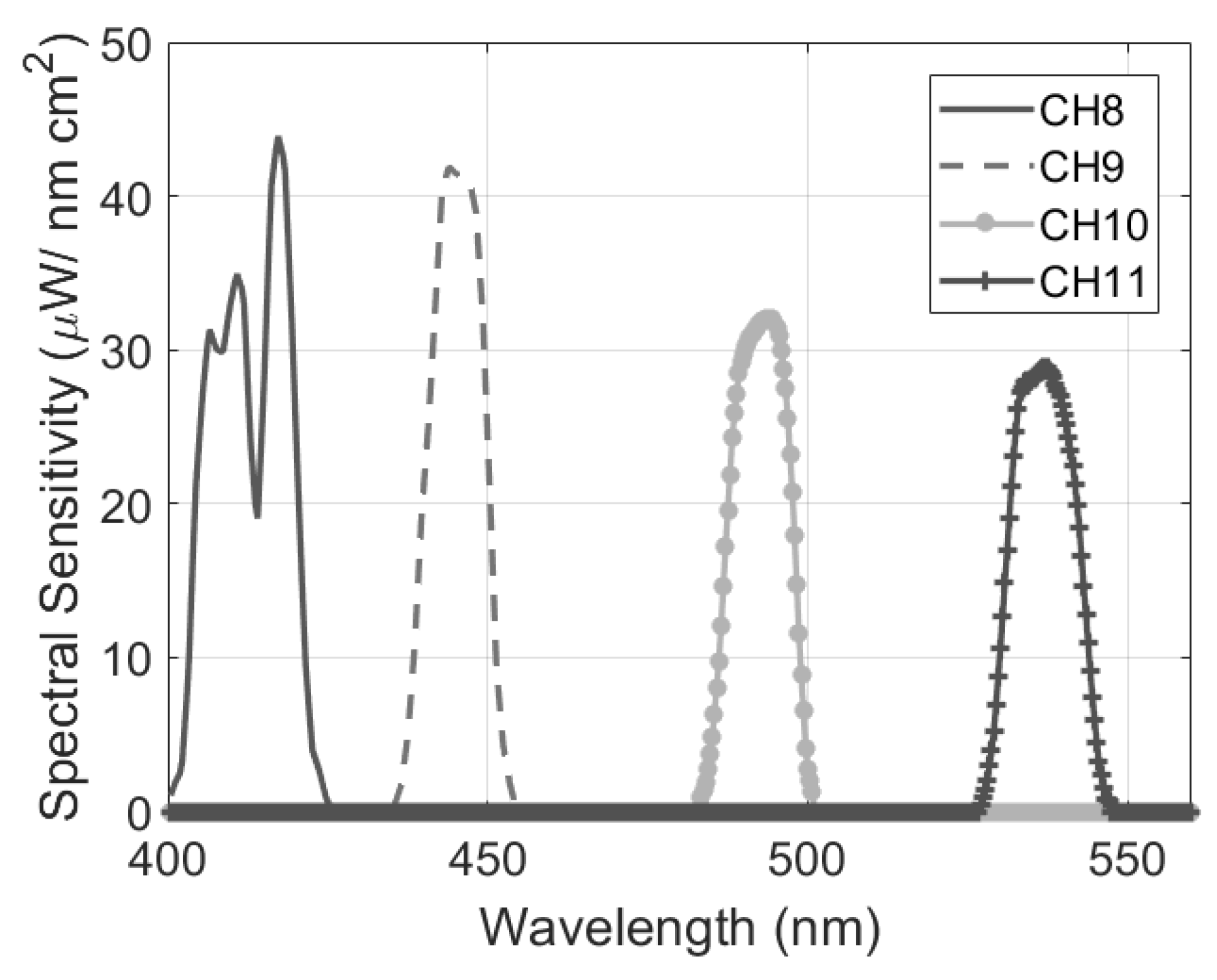
2.1. Remote Sensing with MODIS

The MODIS instrument remotely measures the entire Earth’s surface every 1–2 days, acquiring data in 36 spectral bands ranging in wavelengths from 405 nm–14.4 $\mathsf{\mu }$m. MODIS measures images of the Earth’s surface, in three different spatial resolutions: 250 m, 500 m, and 1 km. Its optical channels allow it to sense spectral information by reflection (typically between Bands 1 and 19) and by radiation (typically infrared bands from Channels 20–36). A more detailed description of the MODIS specification can be found in [42]. Measurements of radiation emitted from the Earth, as well as the radiation reflected from sunlight on the terrestrial surface are recorded as measurements in the IR range. However, during the day, the Earth-emitted radiation in the visible range is negligible compared to the radiation reflected from sunlight. Thus, the reflectance spectra in the visible band have gained real interest. The optical sensor response at each k^th visible optical channel, ${\rho }_k$, is defined as a function of their respective spectral sensitivity ${\omega }_k$ and the incident spectra, E, reflected from the Earth’s surface illuminated by sunlight, which is defined as follows [43,44]:

$${\rho }_k={\int }_{{\lambda }_{min}}^{{\lambda }_{max}}{\omega }_k\left(\lambda \right)·E\left(\lambda \right)d\lambda +e_k,$$

(1)

where $\lambda \in [{\lambda }_{min},{\lambda }_{max}]$ is the spectral sensitivity wavelength range of the k^th optical sensor and $e_k$ represents an additive random noise, mainly given by the electronics’ readout noise and dark current of the detectors [45].

2.2. Spectral Retrieval

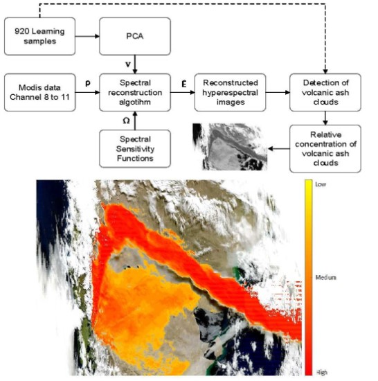
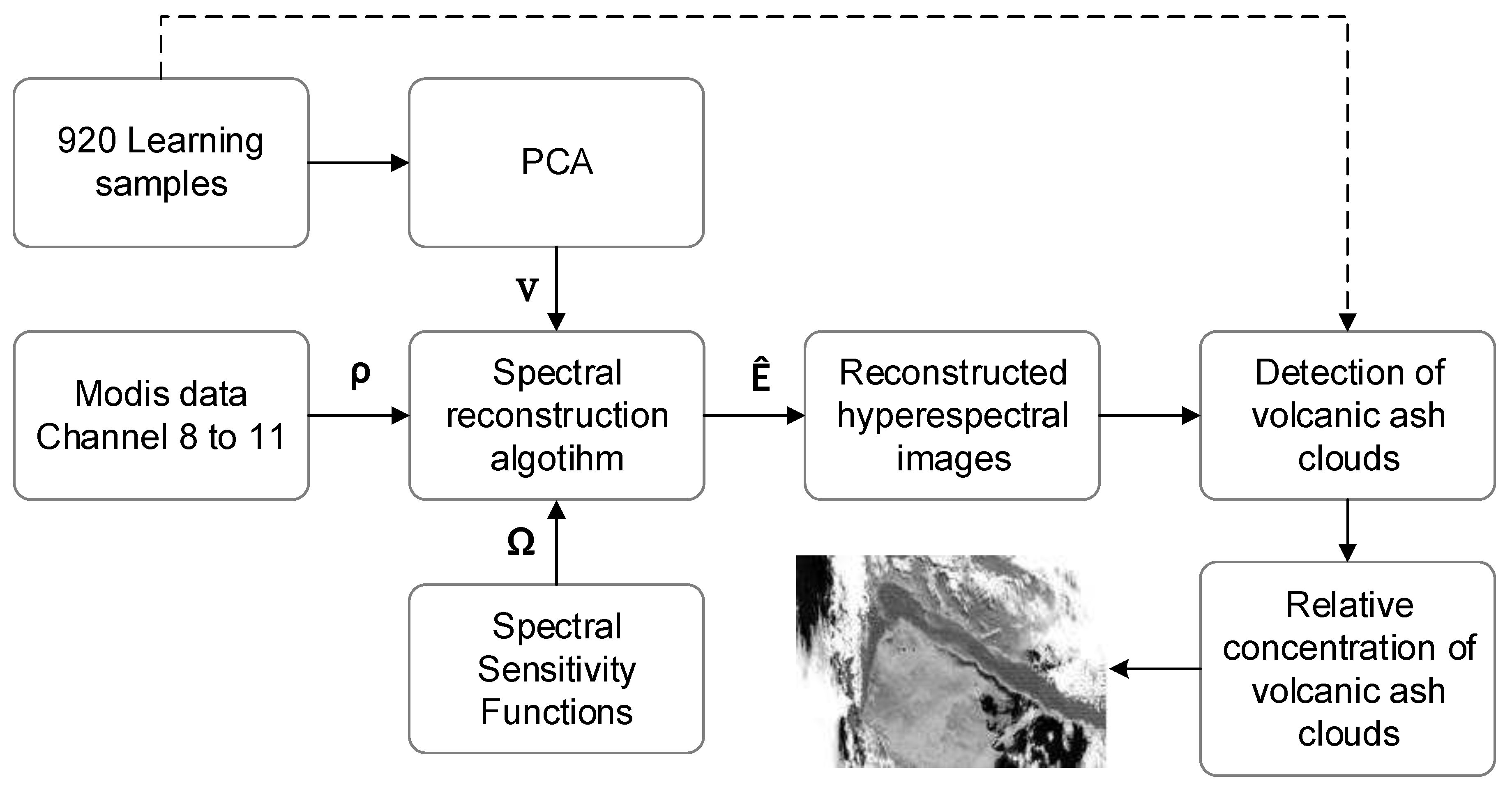
The spectral retrieval or spectral estimation consists of the recovering of high spectral resolution data (at N channels), by using the response of a few optical sensors (k sensors), where typically, $k<<N$. The spectral retrieval is a special case of an ill-posed problem, where additional information from the analyzed phenomenon is required. This additional information consists of a referential database of the phenomenon to be estimated, whose spectral information could be reduced to a few n basis functions [43]. First, let us assume that a high spectral resolution digital spectrometer measures an incident spectrum E at an N wavelength. Assuming a linear behavior of the optical system, then the optical sensor responses in Equation (1) can be represented in matrix notation as:

$$\rho ={\Omega }^{T}E+e,$$

(2)

where $\rho$ is a k-by-one vector containing the optical sensor pixel response, E is an N-by-one column vector representing the incident spectrum, and $\Omega$ is an N-by-k matrix containing the spectral sensitivity vectors of the optical channels (T is the transpose function). In practice, spectral sensitivity vectors in $\Omega$ features any optical sensor in a mathematical way and represents the transmittance of the filters of the optical sensor weighted by its quantum efficiency [46,47]. We will consider that the additive noise e could be neglected and the spectral sensitivity vectors in $\Omega$ are known.

To obtain the spectral retrieval model, let us assume that a set of target spectra of high spectral resolution N have been previously measured and stored in a referential matrix L. This matrix is composed of p uncorrelated samples (sorted in rows) and measured with a high spectral resolution spectrometer; then, the dimension of L is p-by-N. Next, we assume that any spectra in the referential dataset L could be approximated by a linear model as follows [46,48]:

$$E_{ref}=Vϵ,$$

(3)

where $E_{ref}$ is the spectrum defined as a linear combination of the n basis functions, V is an N-by-n matrix containing the n basis vectors able to generate any spectrum in L, and $ϵ$ contains the n unknown coefficients for the linear combination. The linear basis in V is obtained using dimensionality reduction methods, such as principal component analysis (PCA), non-negative matrix factorization (NNMF), or independent component analysis (ICA) [43,44,49]. Dimensionality reduction methods allow retaining most of the spectral information contained in referential dataset L, in a few basis vectors. On the other hand, consider now the presence of a mapping operator G that suitably combines the linear representation in Equation (3) and the optical sensor response $\rho$ on Equation (2), able to minimize the average squared error between any spectrum $E_{ref}$ contained in L and a properly-estimated spectrum. The linear relation between the optical sensor response $\rho$, the mapping operator G, and the estimated spectrum $\widehat{E}$ could be written as follows:

$$\widehat{E}=G\rho .$$

(4)

Then, spectral retrieval is reduced to an optimization problem, where the operator G needs to be calculated. There are two approaches to address this problem, according to the use of referential spectral measurements or the required optical sensor spectral sensitivity function $\Omega$. The first approach does not require the optical sensor sensitivity $\Omega$ [49]. Unfortunately, this method requires simultaneous measurements between referential spectra (L) and the sensors’ channels to calculate the parameters of the mapping operator G, which would not be feasible in the case of volcanic ash reflectance measurements. To surpass this limitation, the second approach incorporates the optical sensor spectral sensitivity $\Omega$. In this context, the Maloney–Wandell method provides a proper estimate of G. This method of spectral retrieval was firstly proposed for spectral characterization of human vision [43,50], and in the last few years, its applications have been extended [44,46,47,48]. Thus, combining Equation (3) and Equation (2), the linear relation $ϵ=\left[{\Omega }^{T}V\right]\rho$ can be found. Then, using this relation in Equation (3), it can be found that matrix $G=V{\left[{\Omega }^{T}V\right]}^{+}$ (where ${}^{+}$ represents matrix pseudo-inverse). Then, replacing G in Equation (4), the retrieval spectra can be computed as:

$$\widehat{E}=V{\left[{\Omega }^{T}V\right]}^{+}\rho .$$

(5)

The Maloney–Wandell method for spectral retrieval provides good results concerning simplicity and accuracy. This approach is restricted by knowledge of information concerning the optical sensor spectral sensitivity $\Omega$, which however is provided by the manufacturers; and the referential dataset of reflectance spectra L, which are not simultaneously measured. In this paper, we used this approach to estimate the ash cloud reflected spectra from the response of the visible optical channels from MODIS, then to compute the ash cloud detection.

3. Methodology

The proposal for volcanic ash monitoring based on MODIS satellite images is schematized in Figure 1. Measurements of the ash reflectance were performed using samples from the Puyehue-Cordon Caulle eruption; the event occurred in 2011 in Chile. Reflectance spectra, at high spectral resolution, were measured using a USB2000 Ocean Optics Inc. spectrometer (calibrated with an HL2000 lamp, Ocean Optics Inc., Dunedin, FL, USA), enabling us to calculate the basis vectors. The spectral resolution of the USB2000 Ocean Optics Inc. spectrometer is $\Delta \lambda \approx$ 0.3 nm, and spectra were measured within the range of 400 nm–600 nm. A total of 360 spectral samples were measured, at different incident angles and distances in order to retain most of the spectral information from uncorrelated samples. Satellite sensors detect the Earth’s surface signals from solar reflections through atmospheric absorption, so the measured ash reflectance spectra were weighted by solar spectral radiance. Solar spectral radiance was measured on a sunny day over a diffuse surface and at different times and angles. Then, reflectance ash samples were weighted by solar spectral radiance, obtaining a training spectral matrix L of 920 reflectance samples. The reflectance spectra of ash samples measured in the laboratory and the obtained training spectra L are shown in Figure 2a,b, respectively.

Linear basis vectors were calculated by using principal components analysis (PCA). PCA was chosen because it has been previously verified to provide the most accurate spectral matching results, using a few of both the optical channels and principal components, compared to the non-negative matrix factorization (NNMF) and independent component analysis (ICA) reduction methods [46,51]. Thus, PCA was computed over the training spectral data L. Figure 3a depicts the first to fourth principal components, as a function of wavelength $\lambda$, where the fourth component and the subsequent basis vectors only contain negligible information. Data representation (in %) is depicted in Figure 3b, calculated as the cumulative variance of the $i^{\mathrm{th}}$ principal component. Data representation allows defining a minimum number of principal components to be used for the spectral retrieval, retaining the overall variability contained in the referential training matrix [44,52]. From Figure 3b, it is observed that using the first four principal components retained 99.85% of the overall information contained in the training matrix of referential ash spectral data.

For computing the spectral retrieval model in Equation (5), the spectral sensitivities of the MODIS sensors, in the visible band, are required. MODIS sensors have seven optical channels between 400 nm and 600 nm (Bands 3, 4, 8, 9, 10, 11, and 12). According to [44], the Maloney–Wandell method provides better accuracy in spectral retrieval when the number of basis vectors matches the number of optical sensors. Then, a key aspect before computing Equation (5) is to find the most proper optical channels. In such a case, we will choose a subset of four channels from the seven available visible channels, where sensors orthogonality is maximized and whose center wavelengths (${\lambda }_c$) are relatively equally spaced [53]. That is, the inner product between the sensitivity curves should be minimized. Defining ${\omega }_i$, $i=1,\dots ,4$, as an optimal optical channel, such as ${\omega }_i\in {\omega }_g$, $g=1,\dots ,7$, and ${\lambda }_c\left(i\right)$ its respective center wavelengths, then the optimal subset of sensors should satisfy the following properties: ${{\omega }_i}^T{\omega }_j=0,\forall i\ne j$, and the step ${\lambda }_c(i+1)-{\lambda }_c\left(i\right)$ should be similar. Thus, the optimal optical channels that satisfy these criteria are Channels 8, 9, 10, and 11. Figure 4 shows the sensitivity of the selected channels, where intensity describes the spectral radiance necessary to saturate each channel.

Finally, to evaluate the performance of the spectral retrieval, the goodness-of-fit coefficient (GFC) and root-mean-squared-error (RMSE) metrics suitable for spectral matching [50] were computed according to Equation (6) and Equation (7), respectively:

$$GFC=\frac{\sum E·\widehat{E}}{\sqrt{\sum E^2·\sum {\widehat{E}}^2}}$$

(6)

$$RMSE=\sqrt{\frac{1}{p}\sum _{j=1}^p{(E_j-\widehat{E_j})}^2}$$

(7)

While GFC compares spectral projection (where a GFC close to 1 means an excellent match), RMSE compares values’ differences over all wavelengths (where an RMSE close to zero means an excellent match).

Relative Ash Concentration

A volcanic ash cloud in an eruption event is spatially dispersed as a function of the wind speed and direction [54], resulting in a non-uniform ash cloud concentration or plume density (in kg/m³). Concerning the interaction between the volcanic ash and the impinging solar radiance, the reflected light is affected mainly by ash absorption and scattering, while in cloud zones with a weak ash concentration, part of the solar radiance is also transmitted to the Earth’s surface [55].

In order to corroborate the relative ash concentration calculation, Figure 5a shows the reflectance of volcanic ash particle samples, measured under different relative concentrations in the line-of-sight (from 1×–5× relative concentrations). In Figure 5b, the integration of the reflectance samples can be seen, over all wavelengths. The results show an increasing value of the integral, according to $a·log\left(x\right)+b$, where a and b are constants. Therefore, while ash samples’ concentration increase, the reflectance of the ash samples also increases, and the ash cloud becomes less transparent [56].

Then, in this work, the relative concentration of the volcanic ash cloud, $R_{ash}$, will be calculated as the integral of the recovered spectrum $\widehat{E}$ in Equation (5), as follows:

$$R_{ash}={\int }_{{\lambda }_{min}}^{{\lambda }_{max}}\widehat{E}\left(\lambda \right)d\lambda$$

(8)

4. Results and Discussion

To corroborate the performance of the spectral recovering model Equation (5), we have tackled three procedures. First, we have simulated the model to identify the proper number of basis vectors that improve the performance of the spectral recovery. We have used for that the same spectra from the training matrix L (Figure 2b) and the selected four optical channels shown in Figure 4. Second, we have computed this model over a synthetic image constructed for such a purpose. The idea is to corroborate that the recovered spectra from other targets exhibit poor GFC metric values. This procedure will allow defining a threshold of the metric values to discriminate between the ash cloud with other targets. Finally, we applied the model for ash cloud detection over MODIS images.

4.1. Computational Results for Ash Reflectance Retrieval

In this step, we have computed the spectral retrieval procedure using the training spectra in L and the selected MODIS channels.

Table 1. Accuracy of the spectral retrieval as a function of principal components (averages values of metrics). GFC, goodness-of-fit coefficient.

PC	GFC	RMSE
1	0.9999	1.0700
2	0.9999	0.8366
3	0.9999	0.7473
4	0.9999	0.7115
5	0.9999	0.8129
6	0.9999	0.8300
7	0.9998	1.1453
8	0.9970	1.4362

summarizes the obtained results of the average values of $GFC$ and $RMSE$, calculated for a different number of principal components (PC). $GFC$ verifies the high accuracy of the spectral retrieval, and $RMSE$ allows corroborating that the best results on the spectral recovery are obtained by using the first four principal components for ash detection.

With these results, it has been verified that in practice, the recovering process provides excellent results when the number of principal components matches the number of optical channels [44]. Hereafter, the four selected MODIS channels and the first four basis vectors for volcanic ash detection will be used.

4.2. Volcanic Ash Detection Validation Using a Synthetic Image

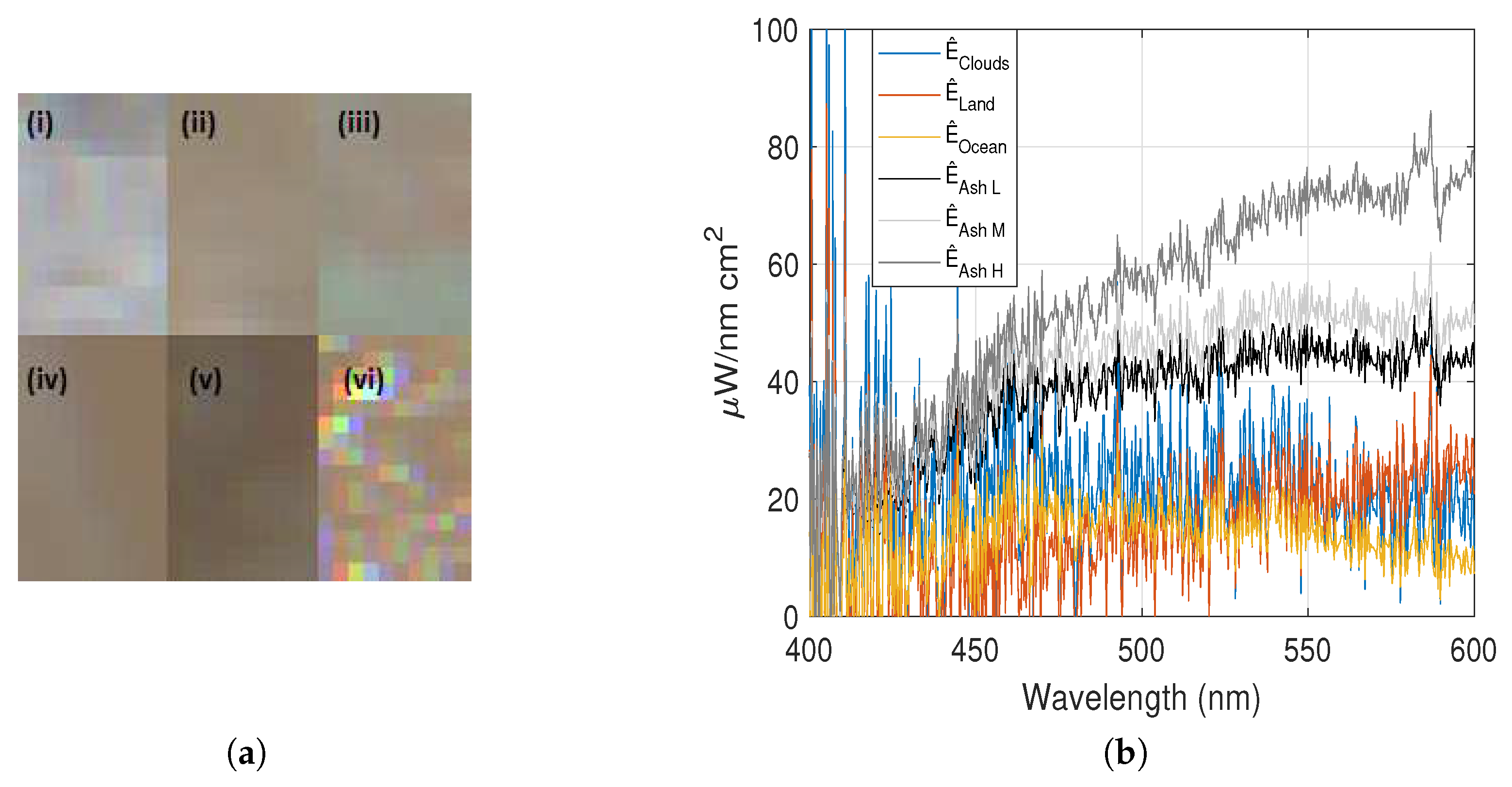
In this step, we have computed the spectral retrieval procedure and the temperature difference method, applied over a synthetic image composed of ash (at different concentrations: Ash H: high density; Ash M: medium density; and Ash L: low density), ocean, land, and water cloud targets. The comparison between both methods was verified by the following procedure:

• A data cube of dimension $N_{pix}\times N_{pix}\times N\times 6$ ($N_{pix}=30$) pixels was composed by data from MODIS Channels 8, 9, 10, 11, 31, and 32, using pixels from different targets (ash clouds at different concentrations, ocean, land, and water clouds, as depicted in Figure 6a).
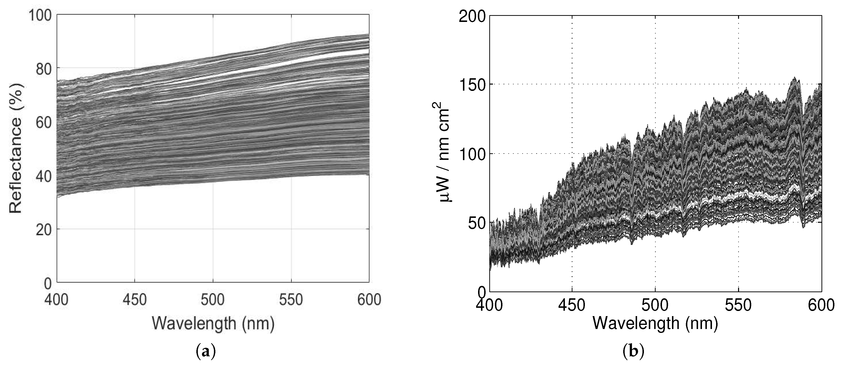
• High-resolution spectra were estimated with the model Equation (5), for each pixel, using the response of MODIS Channels 8, 9, 10, and 11. In Figure 6b is shown the recovered spectra from the different targets. Note the accuracy in the retrieval procedure (compared with the training spectra in Figure 2b) when ash pixels were used with the model, in comparison with the noisy spectra recovered using response channels from other targets.
• GFC was calculated at each pixel, between the estimated high-resolution spectra and the whole spectra contained in the training spectra L. Then, the best GFC was saved. If GFC surpassed a threshold of 0.940, then the pixel was considered as an ash target. Otherwise, the pixel contained information from another target. In parallel, the temperature difference method was computed using MODIS Channels 31 and 32. If temperature differences $T_{31}-T_{32}>-300$, then the pixel would be considered as ash [3].
• A simple binary classification was computed over the entire synthetic image using both the proposed and temperature difference methods. In

  Table 2. Comparison between both the proposed and temperature difference methods, using binary classification (in percentage %).

  Criterion	Performance (%) Proposed Method	Performance (%) Temperature Differences Method
  True positive (ash row)	86.22	99.11
  False positive (ash row)	13.77	0.88
  False negative (other targets row)	29.33	81.77
  True negative (other targets row)	70.66	18.22

  are presented the results (in percentage %).

With these results, it has been verified that the spectral recovering method provides excellent results in detecting ash pixels. Although true positives were fewer than those obtained with the temperature difference method, false negatives were much fewer than the other method, indicating that by means of a spectral comparison, the spectral recovering method is more robust in discriminating and separating pixels from other targets. These results agree with previous studies [3,57].

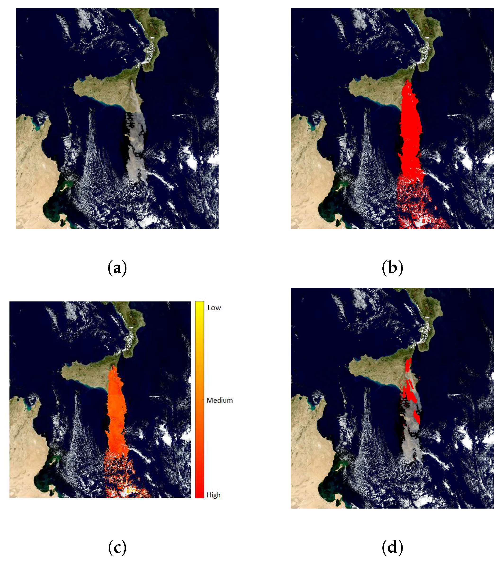
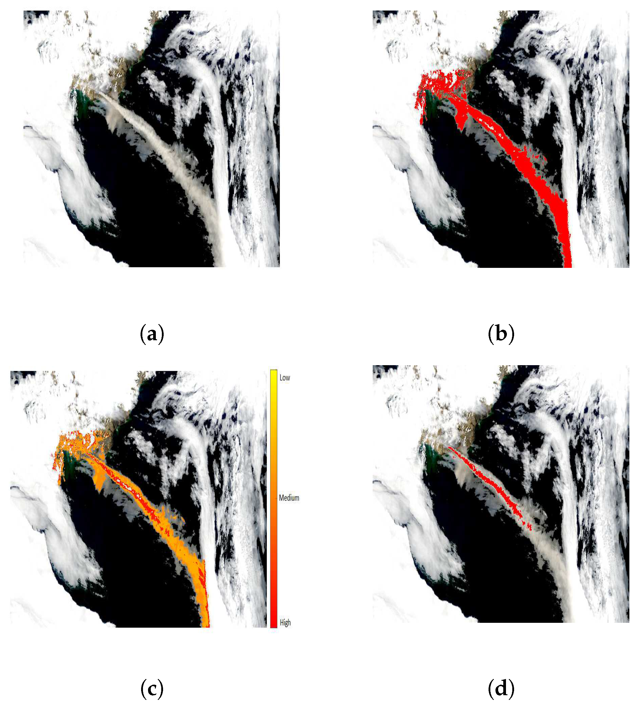
4.3. Volcanic Ash Monitoring Using MODIS Satellite Images

This section presents the obtained results for volcanic ash cloud detection and the relative concentration estimation, based on the spectral retrieval algorithm and the methodology described in Figure 1. Three different events where considered for this evaluation: Puyehue, Chile (40°35′0″S 72°7′0″W), 2011; Etna, Italy (37°45′18″N 14°59′43″E), 2002; and Eyjafjallajökull, Iceland (63°37′48″N, 19°37′12″W), 2010. First, the detection of ash clouds was estimated. This procedure was tackled by calculating a recovered spectrum, pixel-by-pixel, using the response of Channels 8, 9, 10, and 11. Then, the recovered spectrum was compared with all the spectra contained in L (Figure 2b), and the best GFC metric value was saved. If GFC surpassed a threshold of 0.975, then the pixel was considered as an ash target. Otherwise, the pixel contained information from another target. Second, the relative concentration of ash in the cloud was evaluated, by calculating the integral over the recovered spectrum in pixels where ash was detected. Finally, the performance of the volcanic ash cloud detection based on the spectral retrieval was compared to the results obtained using the temperature difference method ([29,58]).

In Figure 7, Figure 8 and Figure 9 are shown the results of the volcanic ash cloud detection methods, from the above-mentioned eruption event. In Figure 7a, Figure 8a, and Figure 9a are shown the composed RGB image from MODIS during the events, as a reference. In Figure 7b, Figure 8b, and Figure 9b are shown the volcanic ash cloud detection results using the proposed approach, exhibiting an excellent detection of the cloud contours, even in zones where ash clouds had a weak concentration and in the presence of water clouds. In Figure 7c, Figure 8c, and Figure 9c are shown the overall results for volcanic ash cloud detection, by calculating the relative ash concentration. Note that in the cases of Figure 7c and Figure 9c, a greater concentration density in the middle of the clouds is clearly highlighted, and the contours revealed a weak concentration. Furthermore, by following the concentration intensity and plume, the zone of the eruption is clearly pointed out in the scene. These results reveal an accurate estimation of the ash cloud and its relative ash concentration, using the spectral recovering model. Instead, Figure 7d, Figure 8d, and Figure 9d reveal that the temperature difference method lacked precision in the contours’ detection of the cloud, also exhibiting great influence when MODIS channels were saturated. This problem of striping noise was strongly eliminated with the proposed approach, because even if any channel used for spectral recovery were saturated, a spectrum with similar spectral characteristics of ash was recovered anyway. Thus, the images resulting from the proposed method (Figure 7c, Figure 8c, and Figure 9c) were based on information provided from various channels, and the influence from any saturated channel was reduced.

4.4. Analysis and Discussion

From the ash spectral retrieval results shown in Table 1, it was verified that the training spectra contained most of the variability in the first four principal components according to the PCA results, due to their highest average values of GFC and smaller average values of the RMSE. Besides, it was verified that in practice, the recovery process provided excellent results when the number of principal components matched the number of optimal optical channels. Then, the first four principal components and the response from MODIS optical Channels 8, 9, 10, and 11 supported the spectral retrieval method for accurately monitoring volcanic ash clouds. Similar results were corroborated by using a constructed synthetic image (see Figure 6) where the performance differences were quantified between spectral retrieval and temperature difference methods. With this last result, the robustness of the proposed method can be concluded, achieving excellent results in detecting true positive ash cloud pixels, notably reducing false alarms. From the ash monitoring results using MODIS images from the Puyehue-Cordon Caulle, Etna, and Eyjafjallajökull eruption events, it was verified that the ash monitoring based on the spectral retrieval method detected ash in the most extended area, clearly revealing the contours and ash density in the clouds, compared to the benchmark temperature difference method. In terms of computer processing time, the spectral retrieval algorithm took 3.81 s to provide an image with a relative ash concentration (processing on a Win10 i7-6700HQ @ 2.6 GHz, 16 GB RAM4 computer). This time was mainly because the recovered spectrum from each pixel should be compared with each spectrum in the training matrix. On the other hand, and similar to the method based on temperature differences, this computational time directly depended on the size of the raw images. By comparing Figure 7c and Figure 7d, it was observed that the proposal was not strongly affected by striping noise, such as in the results from the temperature difference method. This result is due to the fact that even if an optical channel of the MODIS is saturated, the recovered spectrum is also estimated. Moreover, the relative concentration of ash, calculated with Equation (8) improved the information derived with respect to the benchmark temperature difference method, which only reveals ash detection according to the value of the threshold. Subsequently, the results could provide an accurate evaluation of the ash cloud distribution and its relative concentration, even in the presence of water clouds. Then, the method provides an efficient tool for volcanic event monitoring.

5. Conclusions and Future Work

In this work, we proposed a method for hyperspectral retrieval using multispectral satellite images from MODIS, enabling us to monitor ash clouds and their relative concentration accurately when a volcanic eruption event occurs. The core of this method was the measurements of volcanic ash spectral reflectance with a high spectral resolution and enough variance to provide representative information from the process. A total of 920 spectral data from ash samples were used, and this was enough to provide the basis vectors required for spectral retrieval, where the spectral information was concentrated in the first four principal components retaining 99.85% of the overall information. Then, a set of four optimal visible channels from MODIS (Channels 8, 9, 10, and 11) were selected by maximizing the orthogonality and maintaining equal spacing of the center wavelengths. Then, the spectral retrieval was computed pixel-by-pixel, using for that a constructed synthetic image containing different targets and images from different eruption events. Thus, the recovered spectra over the entire images were compared with the spectra in the training matrix. The metrics GFC and RMSE were used for determining the accuracy of the method. Once the ash cloud was detected over the image, a radiometric model based on the integral of the recovered spectrum was applied, enabling us to estimate a relative concentration of ash from the cloud. The results have shown excellent accuracy in the ash cloud estimation, outperforming the temperature difference method classically used for such purposes, providing a complementary tool for daylight monitoring. Future works will consider the ash cloud monitoring based on the proposed method, evaluating incidence on the size of the training matrix and using mixed spectral data from different processes, as well as evaluating the recovering procedure at other spectral bands, to increase the monitoring performance of ash clouds or other remote sensing applications. An important point to be treated in the future will be the definition of an optimization routine to finding an optimum GFC threshold, allowing us to retrieve an optimal image result independent of the ash cloud concentration, as well as to correlate these results with ground-based observations.

References

1. Blaikie, P.; Cannon, T.; Davis, I.; Wisner, B. At Risk: Natural Hazards, People Vulnerability and Disasters, 1st ed.; Routledge: London, UK, 1994; pp. 3–11. [Google Scholar]
2. Prata, A.J. Satellite detection of hazardous volcanic clouds and the risk to global air traffic. Nat. Hazards 2009, 51, 303–324. [Google Scholar] [CrossRef]
3. Pergola, N.; Tramutoli, V.; Marchese, F.; Scaffidi, I.; Lacava, T. Improving volcanic ash cloud detection by a robust satellite technique. Remote Sens. Environ. 2004, 90, 1–22. [Google Scholar] [CrossRef]
4. Longo, B.M.; Rossignol, A.; Green, J.B. Cardiorespiratory health effects associated with sulphurous volcanic air pollution. Public Health 2008, 122, 809–820. [Google Scholar] [CrossRef] [PubMed]
5. Tomašek, I.; Horwell, C.J.; Bisig, C.; Damby, D.E.; Comte, P.; Czerwinski, J.; Petri-Fink, A.; Clift, M.J.; Drasler, B.; Rothen-Rutishauser, B. Respiratory hazard assessment of combined exposure to completegasoline exhaust and respirable volcanic ash in a multicellular humanlung model at the air-liquid interface. Environ. Pollut. 2018, 238, 977–987. [Google Scholar] [CrossRef] [PubMed]
6. Durant, A.J.; Bonadonna, C.; Horwell, C.J. Atmospheric and Environmental Impacts of Volcanic Particulates. Elements 2010, 6, 235. [Google Scholar] [CrossRef]
7. Wilson, G.; Wilson, T.M.; Deligne, N.I.; Cole, J.W. Volcanic hazard impact to critical infrastructure: A review. J. Volcanol. Geotherm. Res. 2014, 286, 148–182. [Google Scholar] [CrossRef]
8. Sparks, R.S.J.; Biggs, J.; Neuberg, J.W. Monitoring Volcanoes. Science 2012, 335, 1310–1311. [Google Scholar] [CrossRef] [PubMed]
9. Lavallée, Y.; Meredith, P.; Dingwell, D.; Hess, K.U.; Wassermann, J.; Cordonnier, B.; Gerik, A.; Kruhl, J. Seismogenic lavas and explosive eruption forecasting. Nature 2008, 453, 507–510. [Google Scholar] [CrossRef] [PubMed]
10. Pavez, A.; Remy, D.; Bonvalot, S.; Diament, M.; Gabalda, G.; Froger, J.L.; Julien, P.; Legrand, D.; Moisset, D. Insight into ground deformations at Lascar volcano (Chile) from SAR interferometry, photogrammetry and GPS data: Implications on volcano dynamics and future space monitoring. Remote Sens. Environ. 2006, 100, 307–320. [Google Scholar] [CrossRef] [Green Version]
11. Menard, G.; Moune, S.; Vlastélic, I.; Aguilera, F.; Valade, S.; Bontemps, M.; González, R. Gas and aerosol emissions from Lascar volcano (Northern Chile): Insights into the origin of gases and their links with the volcanic activity. J. Volcanol. Geotherm. Res. 2014, 287, 51–67. [Google Scholar] [CrossRef]
12. Edmonds, M. New geochemical insights into volcanic degassing. Philos. Trans. R. Soc. Lond. A Math. Phys. Eng. Sci. 2008, 366, 4559–4579. [Google Scholar] [CrossRef] [PubMed]
13. Aiuppa, A.; Burton, M.; Caltabiano, T.; Giudice, G.; Guerrieri, S.; Liuzzo, M.; Murè, F.; Salerno, G. Unusually large magmatic CO2 gas emissions prior to a basaltic paroxysm. Geophys. Res. Lett. 2010, 37. [Google Scholar] [CrossRef]
14. Patrick, M.R.; Orr, T.; Antolik, L.; Lee, L.; Kamibayashi, K. Continuous monitoring of Hawaiian volcanoes with thermal cameras. J. Appl. Volcanol. 2014, 3, 1. [Google Scholar] [CrossRef] [Green Version]
15. Ofeigsson, B.G.; Hooper, A.; Sigmundsson, F.; Sturkell, E.; Grapenthin, R. Deep magma storage at Hekla volcano, Iceland, revealed by InSAR time series analysis. J. Geophys. Res. Solid Earth 2011, 116. [Google Scholar] [CrossRef]
16. Johnson, J.B.; Ripepe, M. Volcano infrasound: A review. J. Volcanol. Geotherm. Res. 2011, 206, 61–69. [Google Scholar] [CrossRef]
17. Pugnaghi, S.; Guerrieri, L.; Corradini, S.; Merucci, L. Real time retrieval of volcanic cloud particles and SO2 by satellite using an improved simplified approach. Atmos. Meas. Tech. 2016, 9, 3053–3062. [Google Scholar] [CrossRef] [Green Version]
18. Francis, P.; Rotheryr, D. Remote sensing of active volcanoes. Annu. Rev. Earth Planet. Sci. 2000, 28, 81–106. [Google Scholar] [CrossRef]
19. Oppenheimer, C. Review article: Volcanological applications of meteorological satellites. Int. J. Remote Sens. 1998, 19, 2829–2864. [Google Scholar] [CrossRef]
20. Corradini, S.; Montopoli, M.; Guerrieri, L.; Ricci, M.; Scollo, S.; Merucci, L.; Marzano, F.; Pugnaghi, S.; Prestifilippo, M.; Ventress, L.; et al. A Multi-Sensor Approach for Volcanic Ash Cloud Retrieval and Eruption Characterization: The 23 November 2013 Etna Lava Fountain. Remote Sens. 2016, 8, 58. [Google Scholar] [CrossRef]
21. Bignami, C.; Corradini, S.; Merucci, L.; De Michele, M.; Raucoules, D.; De Astis, G.; Stramondo, S.; Piedra, J. Multisensor Satellite Monitoring of the 2011 Puyehue-Cordon Caulle Eruption. IEEE J. Appl. Sel. Top. Appl. Earth Obs. Remote Sens. 2014, 7, 2786–2796. [Google Scholar] [CrossRef]
22. Ellrod, G.P.; Connell, B.H.; Hillger, D.W. Improved detection of airborne volcanic ash using multispectral infrared satellite data. J. Geophys. Res. 2003, 108, 4356. [Google Scholar] [CrossRef]
23. Poret, M.; Corradini, S.; Merucci, L.; Costa, A.; Andronico, D.; Montopoli, M.; Vulpiani, G.; Freret-Lorgeril, V. Reconstructing volcanic plume evolution integrating satellite and ground-based data: Application to the 23 November 2013 Etna eruption. Atmos. Chem. Phys. 2018, 18, 4695–4714. [Google Scholar] [CrossRef]
24. Delene, D.J.; Rose, W.I.; Grody, N.C. Remote sensing of volcanic ash clouds using special sensor microwave imager data. J. Geophys. Res. Solid Earth 1996, 101, 11579–11588. [Google Scholar] [CrossRef] [Green Version]
25. Dubuisson, P.; Herbin, H.; Minvielle, F.; Compiègne, M.; Thieuleux, F.; Parol, F.; Pelon, J. Remote sensing of volcanic ash plumes from thermal infrared: A case study analysis from SEVIRI, MODIS and IASI instruments. Atmos. Meas. Tech. 2014, 7, 359–371. [Google Scholar] [CrossRef]
26. Ganci, G.; Bilotta, G.; Cappello, A.; Herault, A.; Del Negro, C. HOTSAT: A Multiplatform system for the thermal monitoring of volcanic activity using satellite data. Geol. Soc. London, Spec. Publ. 2016, 426, 207–221. [Google Scholar] [CrossRef]
27. Laiolo, M.; Coppola, D.; Barahona, F.; Benítez, J.; Cigolini, C.; Escobar, D.; Funes, R.; Gutierrez, E.; Henriquez, B.; Hernandez, A.; et al. Evidences of volcanic unrest on high-temperature fumaroles by satellite thermal monitoring: The case of Santa Ana volcano, El Salvador. J. Volcanol. Geotherm. Res. 2017, 340, 170–179. [Google Scholar] [CrossRef] [Green Version]
28. Plank, S.; Nolde, M.; Richter, R.; Fischer, C.; Martinis, S.; Riedlinger, T.; Schoepfer, E.; Klein, D. Monitoring of the 2015 Villarrica volcano eruption by means of DLR’s experimental TET-1 satellite. Remote Sens. 2018, 10, 1379. [Google Scholar] [CrossRef]
29. Wen, S.; Rose, W.I. Retrieval of sizes and total masses of particles in volcanic clouds using AVHRR bands 4 and 5. J. Geophys. Res. Atmos. 1994, 99, 5421–5431. [Google Scholar] [CrossRef]
30. Ishimoto, H.; Masuda, K.; Fukui, K.; Shimbori, T.; Inazawa, T.; Tuchiyama, H.; Ishii, K.; Sakurai, T. Estimation of the refractive index of volcanic ash from satellite infrared sounder data. Remote Sens. Environ. 2016, 174, 165–180. [Google Scholar] [CrossRef] [Green Version]
31. Marchese, F.; Falconieri, A.; Pergola, N.; Tramutoli, V. Monitoring the Agung (Indonesia) Ash Plume of November 2017 by Means of Infrared Himawari 8 Data. Remote Sens. 2018, 10, 919. [Google Scholar] [CrossRef]
32. Blackett, M. An Overview of Infrared Remote Sensing of Volcanic Activity. J. Imaging 2017, 3, 13. [Google Scholar] [CrossRef]
33. Scheck, L.; Frèrebeau, P.; Buras-Schnell, R.; Mayer, B. A fast radiative transfer method for the simulation of visible satellite imagery. J. Quant. Spectrosc. Radiat. Transf. 2016, 175, 54–67. [Google Scholar] [CrossRef]
34. Pyatkin, V.P.; Rublev, A.N.; Rusin, E.V.; Uspenskii, A.B. A fast radiative transfer model for hyperspectral IR satellite sounders. Pattern Recognit. Image Anal. 2015, 25, 514–516. [Google Scholar] [CrossRef]
35. Stamnes, K.; Tsay, S.C.; Wiscombe, W.; Jayaweera, K. Numerically stable algorithm for discrete-ordinate-method radiative transfer in multiple scattering and emitting layered media. Appl. Opt. 1988, 27, 2502. [Google Scholar] [CrossRef] [PubMed]
36. Spinetti, C.; Corradini, S.; Buongiorno, M.F. Volcanic ash retrieval at Mt. Etna using AVHRR and MODIS data. In Remote Sensing for Environmental Monitoring, GIS Applications, and Geology VII; International Society for Optics and Photonics: Bellingham, WA, USA, 2007; Volume 6749, p. 67491M. [Google Scholar]
37. Wright, R.; Flynn, L.; Garbeil, H.; Harris, A.; Pilger, E. Automated volcanic eruption detection using MODIS. Remote Sens. Environ. 2002, 82, 135–155. [Google Scholar] [CrossRef] [Green Version]
38. Kervyn, M.; Ernst, G.G.J.; Harris, A.J.L.; Belton, F.; Mbede, E.; Jacobs, P. Thermal remote sensing of the low intensity carbonatite volcanism of Oldoinyo Lengai, Tanzania. Int. J. Remote Sens. 2008, 29, 6467–6499. [Google Scholar] [CrossRef]
39. Murphy, S.; Wright, R.; Oppenheimer, C.; Filho, C.S. MODIS and ASTER synergy for characterizing thermal volcanic activity. Remote Sens. Environ. 2013, 131, 195–205. [Google Scholar] [CrossRef]
40. Yamanouchi, T.; Suzuki, K.; Kawaguchi, S. Detection of clouds in Antarctica from infrared multispectral data of AVHRR. J. Meteorol. Soc. Jpn. Ser. II 1987, 65, 949–962. [Google Scholar] [CrossRef]
41. Prata, A. Observations of volcanic ash clouds in the 10–12 μm window using AVHRR/2 data. Int. J. Remote Sens. 1989, 10, 751–761. [Google Scholar] [CrossRef]
42. Ederer, G. 2018. Available online: https://ladsweb.modaps.eosdis.nasa.gov/missions-and-measurements/modis/ (accessed on 15 September 2018).
43. Maloney, L.T.; Wandell, B.A. Color constancy: A method for recovering surface spectral reflectance. J. Opt. Soc. Am. 1986, 3, 29–33. [Google Scholar] [CrossRef]
44. López-Álvarez, M.A.; Hernández-Andrés, J.; Valero, E.M.; Romero, J. Selecting algorithms, sensors, and linear bases for optimum spectral recovery of skylight. J. Opt. Soc. Am. 2007, 24, 942–956. [Google Scholar] [CrossRef]
45. Madhavan, S.; Xiong, X.; Wu, A.; Wenny, B.N.; Chiang, K.; Chen, N.; Wang, Z.; Li, Y. Noise Characterization and Performance of MODIS Thermal Emissive Bands. IEEE Trans. Geosci. Remote Sens. 2016, 54, 3221–3234. [Google Scholar] [CrossRef] [Green Version]
46. Toro, C.; Arias, L.; Torres, S.; Sbarbaro, D. Flame spectra-temperature estimation based on a color imaging camera and a spectral reconstruction technique. Appl. Opt. 2014, 53, 6351–6361. [Google Scholar] [CrossRef] [PubMed]
47. Garcés, H.O.; Arias, L.E.; Rojas, A.J.; Cuevas, J.; Fuentes, A. Combustion Diagnostics by Calibrated Radiation Sensing and Spectral Estimation. IEEE Sens. J. 2017, 17, 5871–5879. [Google Scholar] [CrossRef]
48. López-Álvarez, M.A.; Hernández-Andrés, J.; Romero, J.; Lee, R.L. Designing a practical system for spectral imaging of skylight. Appl. Opt. 2005, 44, 5688–5695. [Google Scholar] [CrossRef] [PubMed]
49. Imai, F.H.; Berns, R.S. Spectral estimation using trichromatic digital cameras. Proc. Int. Symp. Multispectral Imag. Color Reprod. Digit. Arch. 1999, 42, 1–8. [Google Scholar]
50. Maloney, L.T. Evaluation of linear models of surface spectral reflectance with small numbers of parameters. J. Opt. Soc. Am. 1986, 3, 1673–1683. [Google Scholar] [CrossRef]
51. López-Álvarez, M.A.; Hernández-Andrés, J.; Romero, J. Developing an optimum computer-designed multispectral system comprising a monochrome CCD camera and a liquid-crystal tunable filter. Appl. Opt. 2008, 47, 4381–4390. [Google Scholar] [Green Version]
52. Carvajal, R.C.; Arias, L.E.; Garces, H.O.; Sbarbaro, D.G. Comparative Analysis of a Principal Component Analysis-Based and an Artificial Neural Network-Based Method for Baseline Removal. Appl. Spectrosc. 2016, 70, 604–617. [Google Scholar] [CrossRef] [PubMed]
53. Hardeberg, J.Y. Acquisition and Reproduction of Color Images: Colorimetric and Multispectral Approaches; Universal-Publishers: Irvine, CA, USA, 2001; pp. 157–162. [Google Scholar]
54. Vernier, J.P.; Fairlie, T.D.; Murray, J.J.; Tupper, A.; Trepte, C.; Winker, D.; Pelon, J.; Garnier, A.; Jumelet, J.; Pavolonis, M.; et al. An Advanced System to Monitor the 3D Structure of Diffuse Volcanic Ash Clouds. Am. Meteorol. Soc. 2013, 52, 2125–2138. [Google Scholar] [CrossRef]
55. Pflug, B. Estimation of optical thickness of volcanic ash clouds using satellite data. In Remote Sensing of Clouds and the Atmosphere XIV; International Society for Optics and Photonics: Bellingham, WA, USA, 2009; Volume 7475, p. 747517. [Google Scholar]
56. Lee, K.H.; Wong, M.S.; Chung, S.R.; Sohn, E. Improved volcanic ash detection based on a hybrid reverse absorption technique. Atmos. Res. 2014, 143, 31–42. [Google Scholar] [CrossRef]
57. Seftor, C.J.; Hsu, N.C.; Herman, J.R.; Bhartia, P.K.; Torres, O.; Rose, W.I.; Schneider, D.J.; Krotkov, N. Detection of volcanic ash clouds from Nimbus 7/total ozone mapping spectrometer. J. Geophys. Res. Atmos. 1997, 14, 16749–16759. [Google Scholar] [CrossRef]
58. Prata, A.J. Infrared radiative transfer calculations for volcanic ash clouds. Geophys. Res. Lett. 1989, 16, 1293–1296. [Google Scholar] [CrossRef]
Figure 1. Volcanic ash monitoring methodology, based on spectral retrieval and MODIS satellite images.
Remotesensing 11 01393 g001
Figure 2. (a) Volcanic ash reflectance (in %) measured in the laboratory and (b) training spectral data L, as measured by the satellite.
Remotesensing 11 01393 g002
Figure 3. (a) First four principal components for referential ash reflectance data. (b) Accumulated variance by incrementing the number of principal components.
Remotesensing 11 01393 g003
Figure 4. Spectral sensitivity of the MODIS satellite.
Remotesensing 11 01393 g004
Figure 5. (a) Reflectance of volcanic ash at different concentrations. (b) Integral results over the measured spectral band.
Remotesensing 11 01393 g005
Figure 6. Validation of spectral retrieval with a synthetic image. (a) Synthetic image constructed using (i) ash cloud pixels at high density (Ash H), (ii) ash cloud pixels at medium density (Ash M), (iii) ash cloud pixels at low density (Ash L), (iv) pixels from the ocean target, (v) pixels from land target, and (vi) pixels from water cloud target. (b) Recovered spectra with the proposed method (in μ W/cm2 nm) using VIS channel responses from the synthetic image.
Remotesensing 11 01393 g006
Figure 7. Result comparison from the Puyehue-Cordon Caulle eruption, Chile, 2011. (a) Composed RGB MODIS image during the event. (b) Detection of volcanic ash cloud based on spectral retrieval. (c) Ash cloud monitoring and relative concentration. (d) Temperature difference method results.
Remotesensing 11 01393 g007
Figure 8. Result comparison from the Etna Volcano eruption, Italy, 2002. (a) Composed RGB MODIS image during the event. (b) Detection of volcanic ash based on spectral retrieval. (c) Ash cloud monitoring and relative concentration. (d) Temperature difference method.
Remotesensing 11 01393 g008
Figure 9. Results of ash monitoring from the Eyjafjallajökull Volcano eruption, Iceland, 2010. (a) Composed RGB MODIS image during the event. (b) Detection of volcanic ash based on spectral retrieval. (c) Ash cloud monitoring and relative concentration. (d) Temperature difference method.
Remotesensing 11 01393 g009