Article

Applications of QC and Merged Doppler Spectral Density Data from Ka-Band Cloud Radar to Microphysics Retrieval and Comparison with Airplane in Situ Observation

1
State Key Laboratory of Severe Weather, Chinese Academy of Meteorological Sciences, Beijing 100086, China
2
Hebei Weather Modification Center, Shijiazhuang 610225, China
3
Anhui Sun-Create Electronics Ltd. Co., Hefei 230088, China
*
Author to whom correspondence should be addressed.
Remote Sens. 2019, 11(13), 1595; https://0-doi-org.brum.beds.ac.uk/10.3390/rs11131595
Submission received: 15 May 2019 / Revised: 27 June 2019 / Accepted: 28 June 2019 / Published: 4 July 2019
(This article belongs to the Special Issue Remote Sensing of Clouds)

Abstract

:
The new Chinese Ka-band solid-state transmitter cloud radar (CR) uses four operational modes with different pulse widths and coherent integration and non-coherent integration numbers to meet long-term cloud measurement requirements. The CR and an instrument-equipped aircraft were used to observe clouds and precipitation on the east side of Taihang Mountain in Hebei Province in 2018. To resolve the data quality problems caused by attenuation in the precipitation area; we focused on developing an algorithm for attenuation correction based on rain drop size distribution (DSD) retrieved from the merged Doppler spectral density data of the four operational modes following data quality control (QC). After dealiasing Doppler velocity and removal of range sidelobe artifacts; we merged the four types of Doppler spectral density data. Vertical air speed and DSD are retrieved from the merged Doppler spectral density data. Finally, we conducted attenuation correction of Doppler spectral density data and recalculated Doppler moments such as reflectivity; radial velocity; and spectral width. We evaluated the consistencies of reflectivity spectra from the four operational modes and DSD retrieval performance using airborne in situ observation. We drew three conclusions: First, the four operational modes observed similar reflectivity and velocity for clouds and low-velocity solid hydrometeors; however; three times of coherent integration underestimated Doppler reflectivity spectra for velocities greater than 2 m s−1. Reflectivity spectra were also underestimated for low signal-to-noise ratios in the low-sensitivity operational mode. Second, QC successfully dealiased Doppler velocity and removed range sidelobe artifacts; and merging of the reflectivity spectra mitigated the effects of coherent integration and pulse compression on radar data. Lastly, the CR observed similar DSD and liquid water content vertical profiles to airborne in situ observations. Comparing CR and aircraft data yielded uncertainty due to differences in observation space and temporal and spatial resolutions of the data.

Graphical Abstract

1. Introduction

A Ka-band cloud radar (CR) with a solid-state transmitter using pulse compression, coherent integration, and incoherent integration in several operational modes can detect clouds and precipitation at varying heights and intensities. However, sidelobes from pulse compression cause artifacts, thus increasing the minimum detection range. Additionally, underestimate of the return power through the coherent integration circuitry was not negligible as the particle velocities with respect to the radar approached the radar Nyquist velocity [1]. Coherent integration’s effects on reflectivity estimation were corrected using a power transfer function through coherent integration, and sidelobe artifacts were distinguished using non-range-corrected return power as proposed by Moran et al. [2]. Clothiaux et al. proposed a radar data-processing algorithm to unalias radial velocity aliasing, remove both second-trip echoes and pulse compression sidelobes, and merge reflectivity and velocity from different operational modes [3]. In those works, millimeter wavelength CR (MMCR) recorded three Doppler spectra moments (i.e., reflectivity, velocity, and spectral width) and discarded the Doppler spectra. Kollias further improved MMCR operational modes to record Doppler spectra using a fast Fourier transform (FFT) and presented new methods for postprocessing Doppler spectra to reproduce reflectivity, velocity, and spectrum width [4]. In Kollias’ work, precipitation attenuation was not corrected and coherent integration effects on Doppler spectral data were not discussed.
Before the recording of Doppler spectral density data, vertical air motion has often been retrieved on the basis of a fixed empirical relationship between radar reflectivity and hydrometeor terminal velocity [5,6]. However, establishing a straightforward relationship among these variables has been difficult and thus is not known in the case of thunderclouds [7].
Lhermitte first proposed a methodology for retrieving vertical air motion from Doppler spectral density data that Kollias verified and applied to the study of strong convective precipitation [8,9]. Vertical air velocity can be directly estimated using the velocity bin of small particles such as liquid droplets and small ice crystals; therefore, these particles can be considered tracers of clear-air motion in the measured spectra [10,11,12,13]. This method neglects tracer terminal velocity and turbulence and wind shear effects on Doppler spectral density. The short pulse width, very narrow antenna beam, and high temporal sampling result in a tiny sampling volume compared with those conventional radars and wind profilers. This high resolution is critical for minimizing turbulence and wind shear effects on vertical air speed and drop size distribution (DSD) retrieval [14]. Once air motion is estimated, the Doppler spectrum is shifted to correspond to zero vertical air motion, the actual DSD in stratiform precipitation can be retrieved from the Doppler spectrum under the assumption that turbulence effects on Doppler spectral density data are negligible [15,16,17,18]. However, in drizzling precipitation with small hydrometeors, spectral broadening of turbulence is not negligible. Thus, a forward modeling algorithm for DSD retrieval for drizzling stratiform clouds was proposed considering the spectral broadening of turbulence [19].
In recent years, magnetrons and high-power traveling wave guides have been adopted in transmitters for millimeter-wave radars in China. Doppler spectral density data observed using a Ka-band CR with traveling wave tubes were analyzed and used to retrieve stratiform precipitation DSDs [17]. In 2013, a Ka-band millimeter-wave CR with a solid-state transmitter was developed to obtain continuous and reliable cloud and precipitation measurements. This radar adopted pulse compression and coherent and incoherent integration techniques in three operation modes. The consistency of radar reflectivity, velocity, and Doppler spectral density measured in the different modes was analyzed, and an algorithm integrating reflectivity, velocity, and spectral width from various operational modes was proposed [20,21]. Doppler spectra obtained from single-mode operation were used to retrieve high-resolution vertical air velocities in convective clouds over the Tibetan Plateau based on the “small-particle-traced” idea [7]. However, there were large reflectivity sensibility gaps of 20.8 dB between the precipitation mode and cirrus mode, which limit cloud observations below 2 km height. The merged Doppler spectral data were not used to retrieve DSD, and the retrieved DSD was not evaluated by airborne in situ observation.
In 2017, the Chinese Academy of Meteorological Science (CAMS) and Anhui Sun Create Electronics Co., Ltd., co-developed a new CR with a solid-state transmitter intended to improve the gaps between various modes. This CR operated with four modes and was used to observe cloud and precipitation vertical structures in northern China. Additionally, airborne in situ observation of stratiform precipitation microphysical parameters was conducted using a Beechcraft King Air 350 aircraft operated by the Hebei Province Weather Modification Office.
In this study, we introduce the newly developed Ka-band millimeter wave radar’s major technical and operational parameters and the design of its operational modes. We examined the consistency of Doppler spectra and moments of Doppler spectra measured in various modes to investigate the radar’s detection capabilities as well as biases from different operational modes. Vertical air motion and rain DSD are retrieved using recalculated and merged Doppler spectra, and attenuation correction with DSD are proposed. Additionally, retrieved DSD and water content at various levels are compared with airborne in situ observations.

2. Materials and Methods

2.1. Data and Instrument Descriptions

2.1.1. Cloud Radar

Intensive cloud and precipitation observations were conducted at the Huangsi Meteorological Station in Hebei Province (114.21°E, 37.10°N) May 15–June 30, 2018. The Ka-band CR with solid-state transmitter used in this experiment employs Doppler radar and polarization radar technology and operates in a vertically pointing mode to obtain vertical profiles of reflectivity (Z), radial velocity (Vr), velocity spectrum width (Sw), and the linear depolarization ratio (LDR) in clouds and light precipitation. Meanwhile, it records Doppler spectral density data (SP). Table 1 lists the radar’s major technical parameters, and Table 2 shows subsystem parameters for the CR. The main purpose of using a solid-state transmitter is realizing continuous measurement, as statistical cloud characteristics are especially important in cloud and precipitation physics.
Detecting weak clouds requires special radar techniques. The CR addresses this issue by using different operational modes that can be repetitively cycled. Some operational modes use pulse compression techniques with long pulses to boost radar sensitivity, which enables the detection of weakly reflecting clouds, whereas other operational modes use short conventional pulses. When combined, data from different operational modes can yield a comprehensive and accurate depiction of most of the clouds in a vertical column above the radar. To improve radar detection capabilities for clouds and precipitation, four operational modes are applied: precipitation mode (M1), boundary mode (M2), middle level mode (M3), and cirrus mode (M4). Varying radar pulse widths and coherent and incoherent integration techniques are used to enable detection of low-level cloud and high-level weak clouds (see Table 3 for major operational parameters).
More importantly, coherent integration is applied before FFT, and the FFTs are then incoherently averaged to improve radar sensitivity. M1 with low sensitivity for reflectivity and large Nyquist velocity is important for precipitation studies. In comparison, in other modes, a frequency modulation (FM) long pulse waveform (0.3 km, 1.2 km and 3.0 km pulse widths for M2, M3 and M4 respectively) with a pulse compression ratio of 10, 40 and 100 are used, and two or three times of coherent integration are performed; theoretically, the minimum detectable reflectivity is reduced by 14.7, 20.8 and 23.0 dB, however, the range sidelobe artifacts is produced near the strong reflectivity. These operational modes alternate during CR observations. Once radial measurements are complete in one mode, the CR immediately switches to another mode. Operational mode dwell times (i.e., the time to obtain a radial measurement) are approximately 4 s. Therefore, one complete cycle of all four operational modes will take 16 s.
More importantly, coherent integration is applied before the FFT is performed, and FFTs are then incoherently averaged to improve radar sensitivity. M1, which has low sensitivity and short minimum detective range, without coherent integration and pulse compression and, is suitable for precipitation observation. In comparison, M4, which has high sensitivity and a large minimum detective range, is designed for weak cloud observations and radiation studies; however, it cannot be used to observe clouds and precipitation below 3.0 km. Therefore, a frequency modulation long-pulse waveform (3.0 km pulse width) with a pulse compression ratio of 100 is used and three coherent integrations are performed in M4. This theoretically reduces the minimum detectable reflectivity by 24.8 dB (10log (3 × 100)); however, range sidelobe artifacts are produced near strong reflectivity at a range of 3.0 km. CR added a new mode, M3, to reduce radar sensitivity gaps between different modes below 3.0 km. Reflectivity sensitivity gaps at 2.1 km are about 20.8 dB for the first CAMS CR, but for the new CR, the gaps at 0.3, 1.2, and 3.0 km are 13.5, 6.0, and 2.0 dB, respectively.

2.1.2. Aircraft Instruments

The primary instruments in the aircraft included a modified cloud combination probe (CCP), a two-dimensional stereo probe (2DS),a high-volume precipitation spectrometer (HVPS),and an Aircraft Integrated Meteorological Measurement System (AIMMS-20). The CCP, manufactured by Droplet Measurement Technologies (2400 Trade Centre Avenue Longmont, CO 80503 USA ), consists of a cloud droplet probe (CDP), a grayscale optical array imaging probe (CIPgs), and a hotwire liquid water content (LWC) sensor. The CDP measures cloud droplet concentration in 30 size bins for diameters of 2–50 μm with 1–2 μm resolutions at 1 Hz, which corresponds to a spatial distance of ~100 m. Using a two-dimensional shadow cast technique, the CIPgs detects cloud particles ranging from 15 to 2000 μm in diameter. The 2DS, manufactured by the Stratton Park Engineering Corporation, is an optical array imaging probe that records projected areas of three-dimensional ice particles as well as particle size distributions from 10 to 1280 μm with resolutions of 10, 20, 50, 100 and 200 μm. To mitigate the ice crystal shattering problem, we modified the probe tips and applied the arrival time algorithm to collected sampling to remove artifacts. HVPS data cover the range from 150 to 47,075 μm with resolutions of 150 and 300 μm. Below this range, 2D-S data are used. We computed LWC in this paper by using 2D-S, CIP and HVPS data and compared with those by hotwire and radar data. AIMMS-20 provided meteorological data such as three-dimensional wind vectors, three-dimensional aircraft position (i.e., latitude, longitude, and altitude), ambient temperature, and ambient relative humidity [22]. The aircraft took off from Zhengding Airport and flew over the CR installation for vertical in situ observation between 600 and 4800 m. Widespread stratiform precipitation was observed by the CR and the aircraft. Between 1317 and 1349 China Standard Time (CST) May 21, 2018, the aircraft reached a maximum altitude of 4800 m and spiraled downward to 700 m around the CR observation site to observe cloud and precipitation vertical structures.

2.2. Data Processing Methods

We developed an attenuation correction based on algorithms for dealiasing singly wrapped aliased Doppler spectral density, detecting and removing artifacts produced by pulse compression, and merging reflectivity spectra [21] using DSD retrieved from Doppler spectral density to reduce the attenuation effects on reflectivity. Quality control (QC) for Doppler spectra includes dealiasing singly wrapped aliased Doppler spectral density data and detecting and removing artifacts produced by pulse compression. The merged reflectivity spectra from the four operational modes previously mentioned filled in gaps during periods of weak clouds, reduced the effects of coherent integration and pulse compression in liquid precipitation, mitigated Doppler velocity aliasing, and removed artifacts. After QC and merging Doppler spectral density, we conducted attenuation correction of Doppler spectral density bin by bin from the first range to the end. We calculated the attenuation coefficient from DSD, which reduces the effects of uncertainty of reflectivity and the attenuation coefficient relationship on attenuation correction.
For each beam, we calculated DSD in the first valid bin using the raw merged Doppler spectral density and calculated the one-way attenuation rate (dB/km) K by integrating a specified extinction cross section and DSD over drop diameters based on Doviak and Zrnic´s Equation (3.15) [23]:
K i = 0.4343 j = 1 n Q T H ( D j ) N ( D j ) Δ D
Here, QTH (cm2) is the extinction cross section by extended boundary condition [24], N(D) (mm−1 m−3) is the DSD retrieved from Doppler spectral density, and D is hydrometeor diameter.
Let SZm(n, i) and SZc(n, i) represent the raw and attenuation-corrected Doppler spectral bins at the n-th FFT bin in the i-th radar sample volume. Attenuation correction is thus calculated by:
S Z c ( n , i ) = S Z m ( n , i ) exp ( 0.2 K j Δ R )
For any value of i that satisfies i > j. After producing attenuation-corrected Doppler spectral density at the second range bin, DSD and the attenuation coefficient are retrieved from the attenuation-corrected Doppler spectral density. Finally, the Doppler spectral densities above the range are produced.
Reflectivity, radial velocity, and spectral width are then recalculated from the merged reflectivity spectrum SZm:
Z m ( R ) = i = 1 n S Z m ( i , R ) Δ V i
V r m ( R ) = i = 1 n V i S Z m ( i , R ) Δ V i i = 1 n S Z m ( i , R ) Δ V i
S w m ( R ) = i = 1 n ( V i V r m ( R ) ) 2 S Z m ( i , R ) Δ V i i = 1 n S Z m ( i , R ) Δ V i 1 / 2
Here, n is the number of FFT points (256); SZm (i, R) is the merged reflectivity spectra for the i-th FFT bin at the range gate of R; Δ Vi is the corresponding velocity spacing; and Zm, Vrm, and Swm are reflectivity, radial velocity, and spectral width, respectively.

3. Results

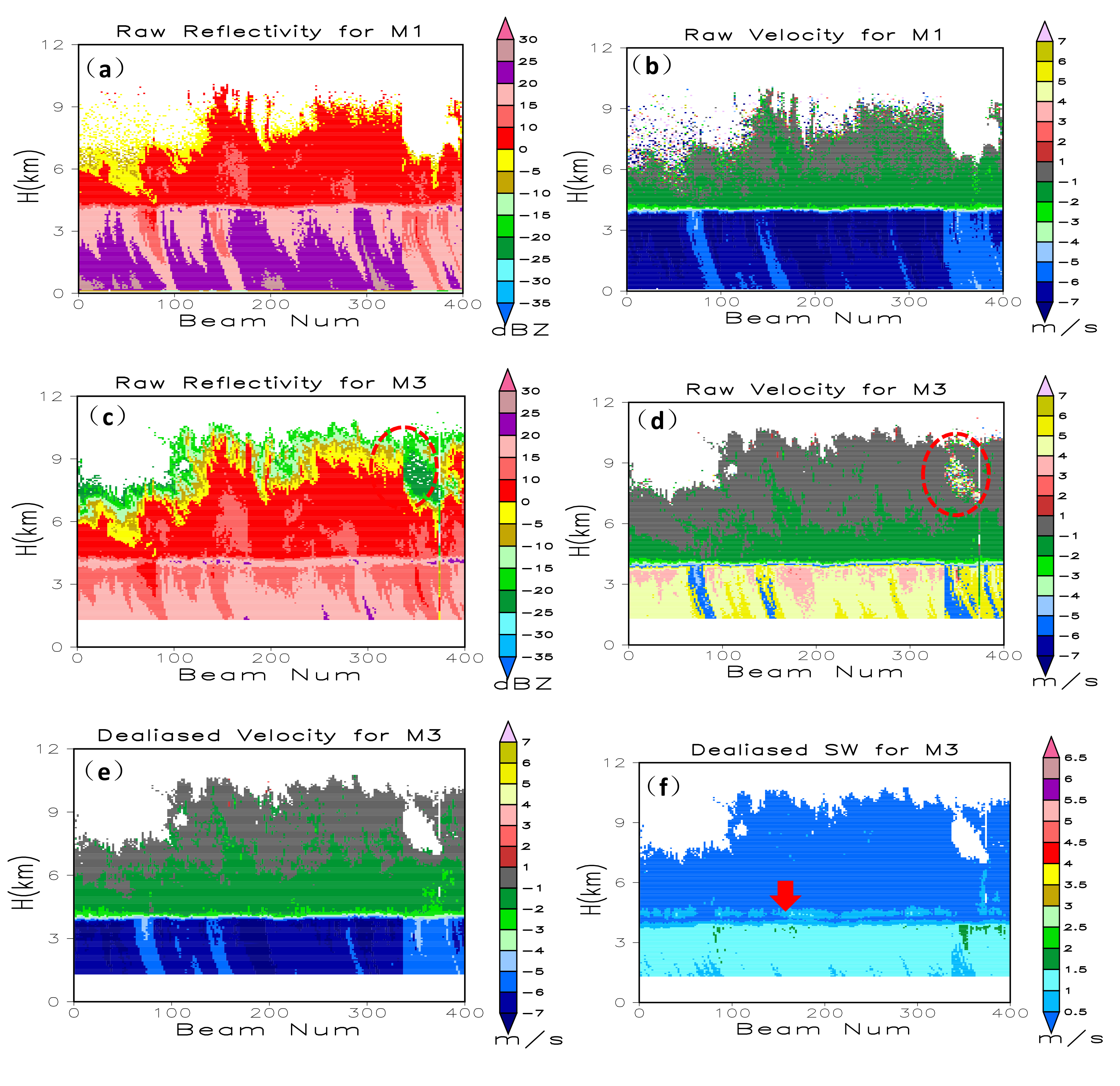
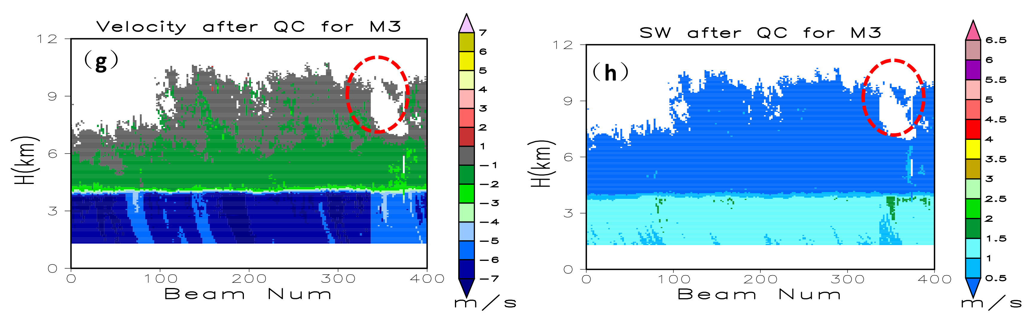
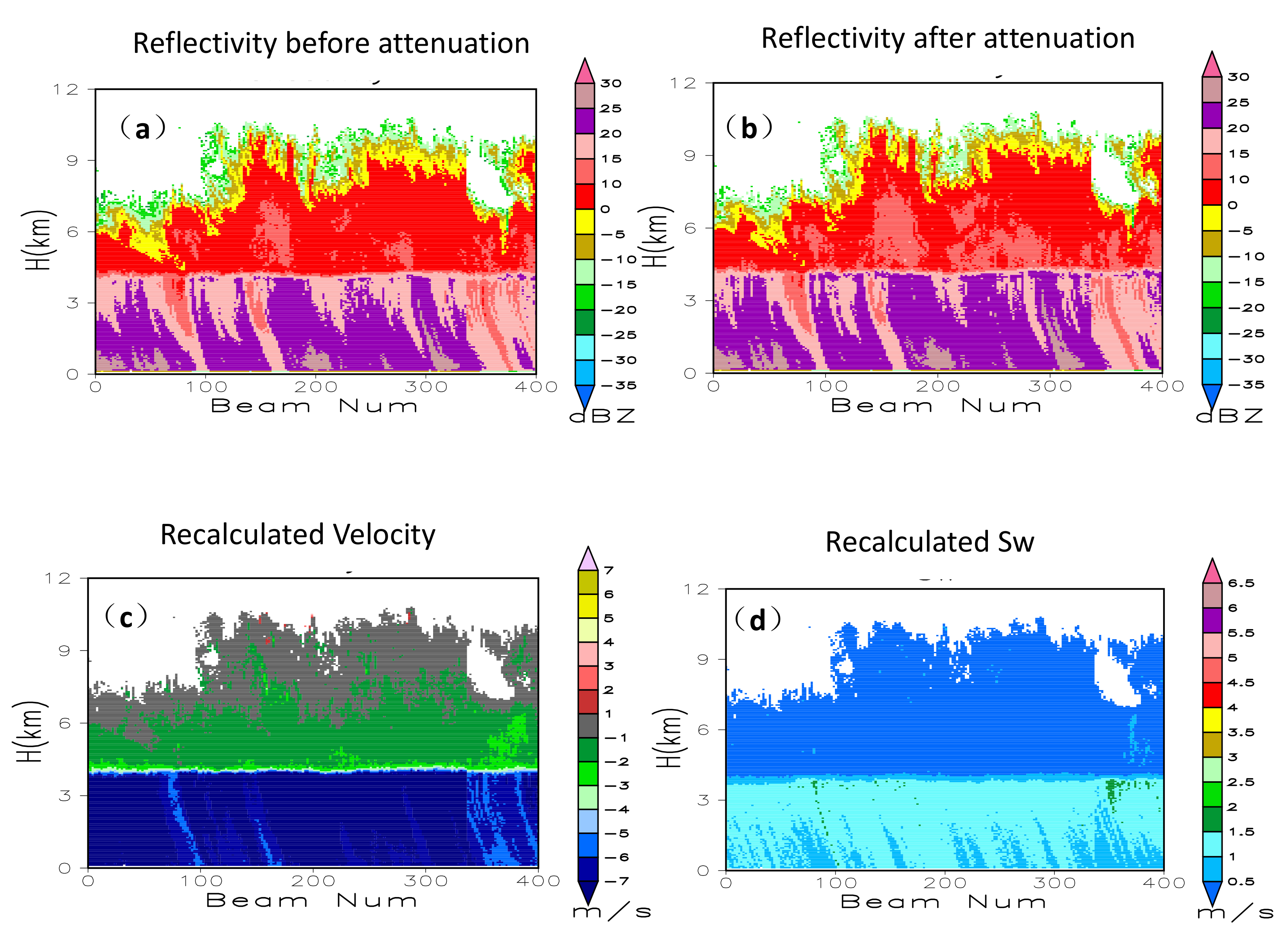
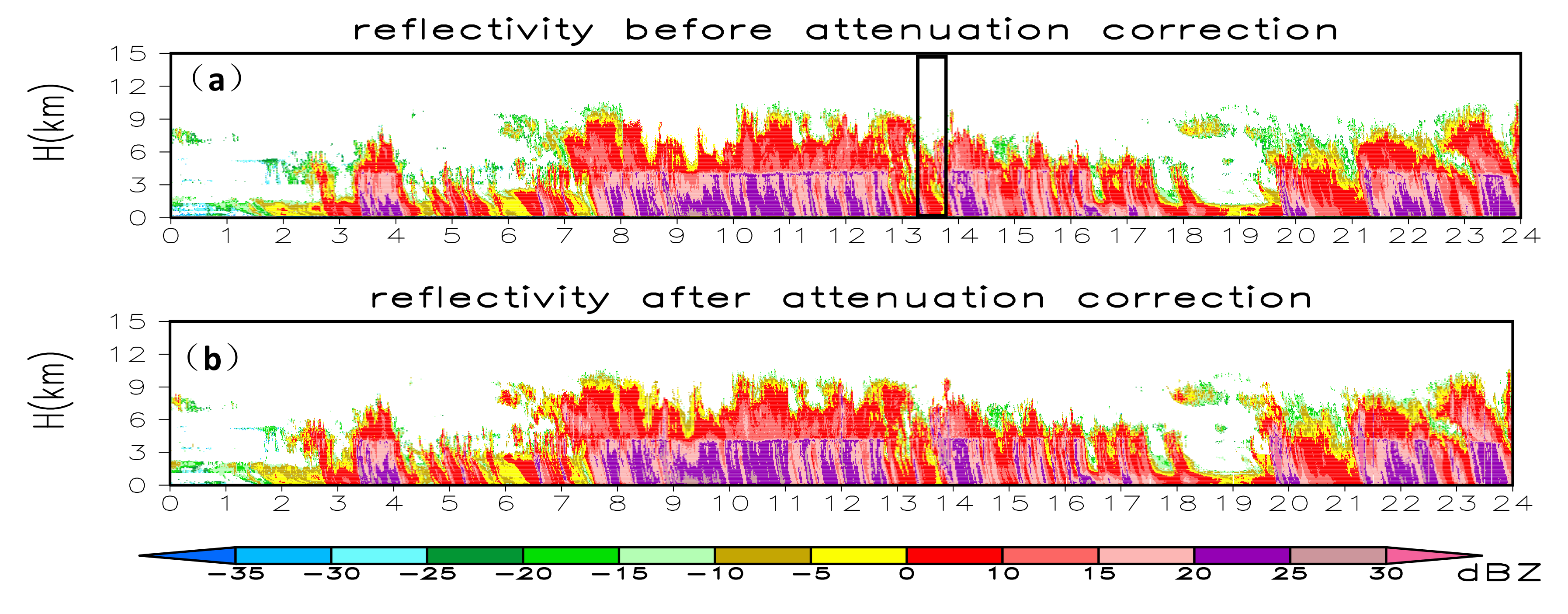
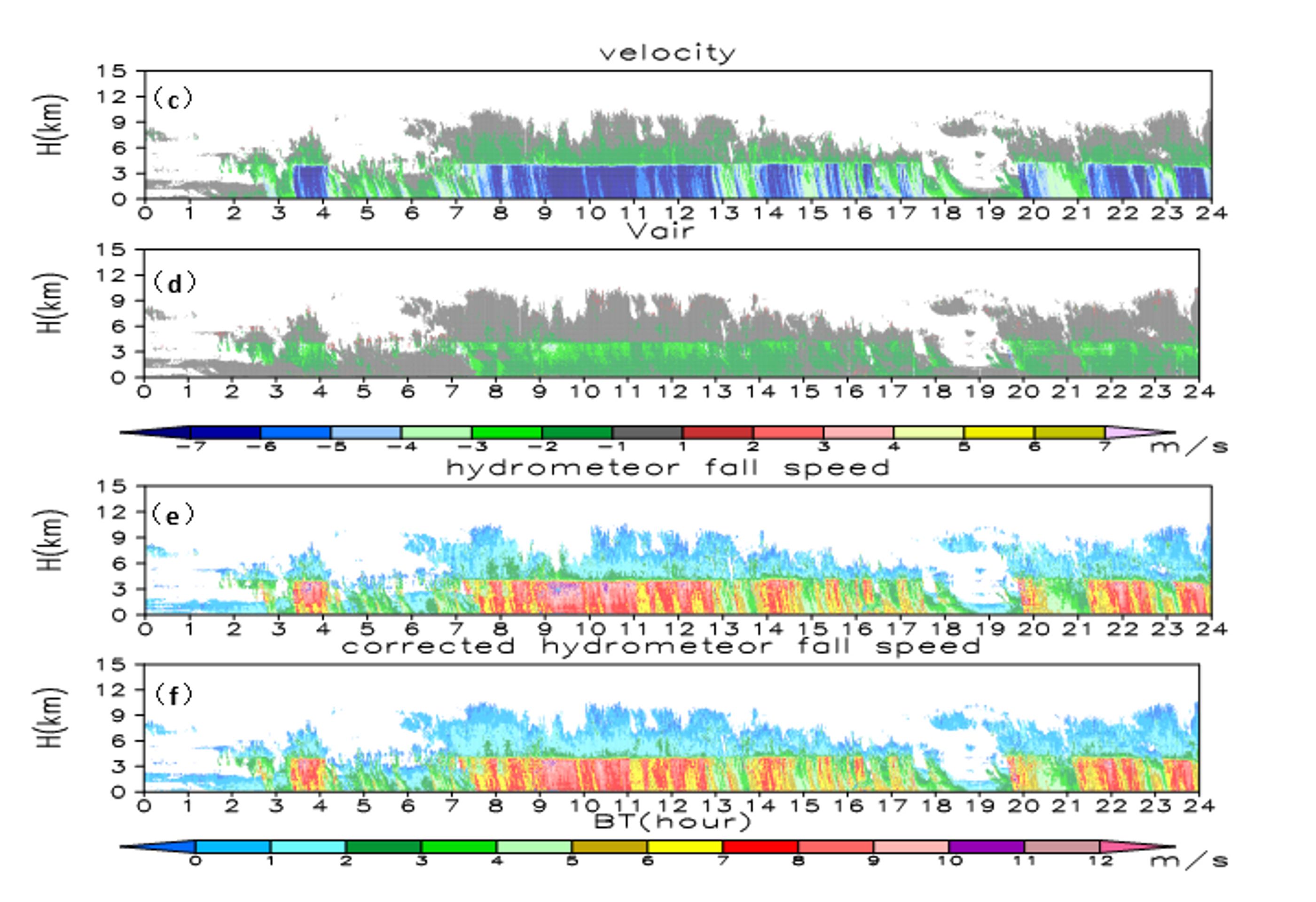
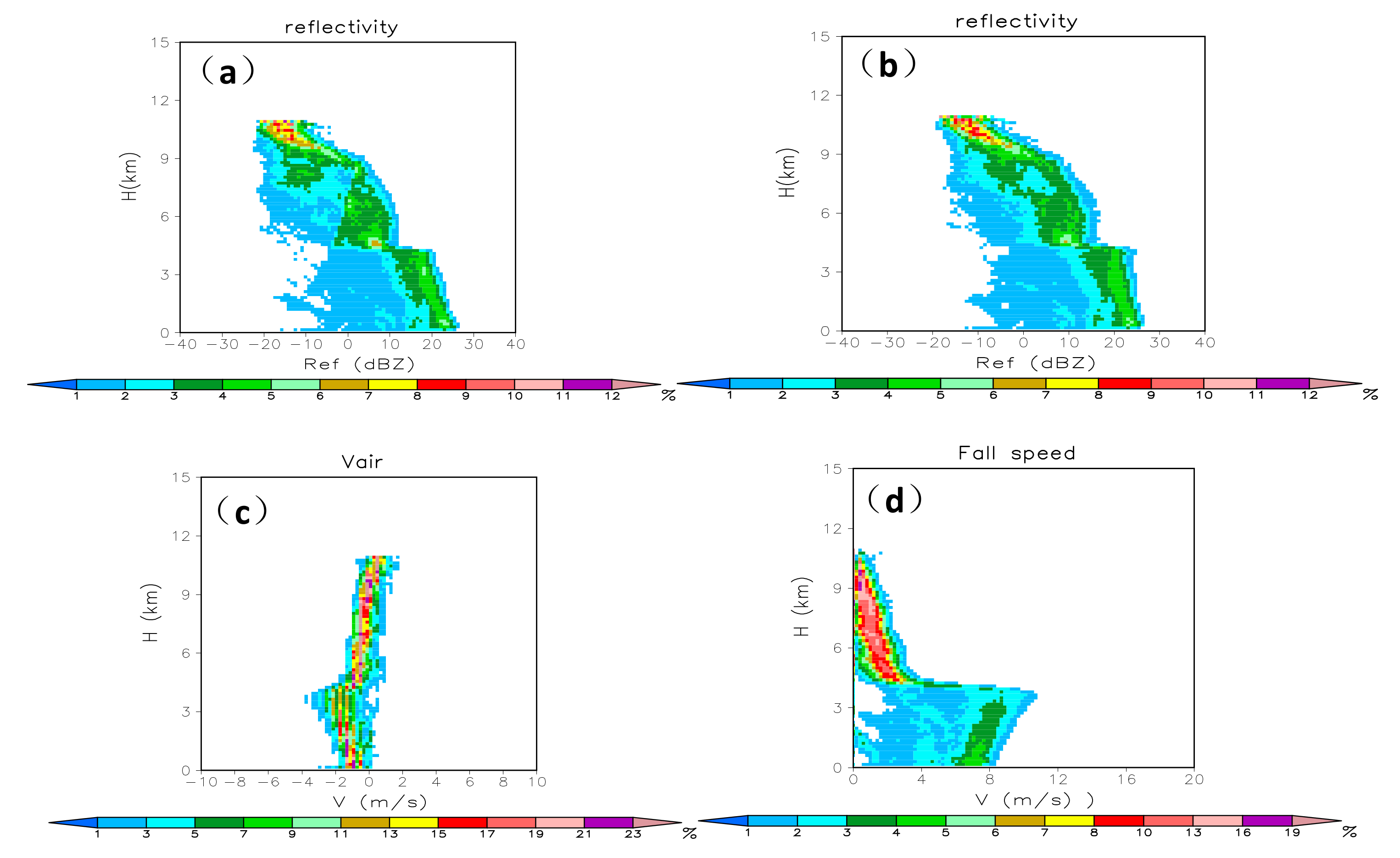
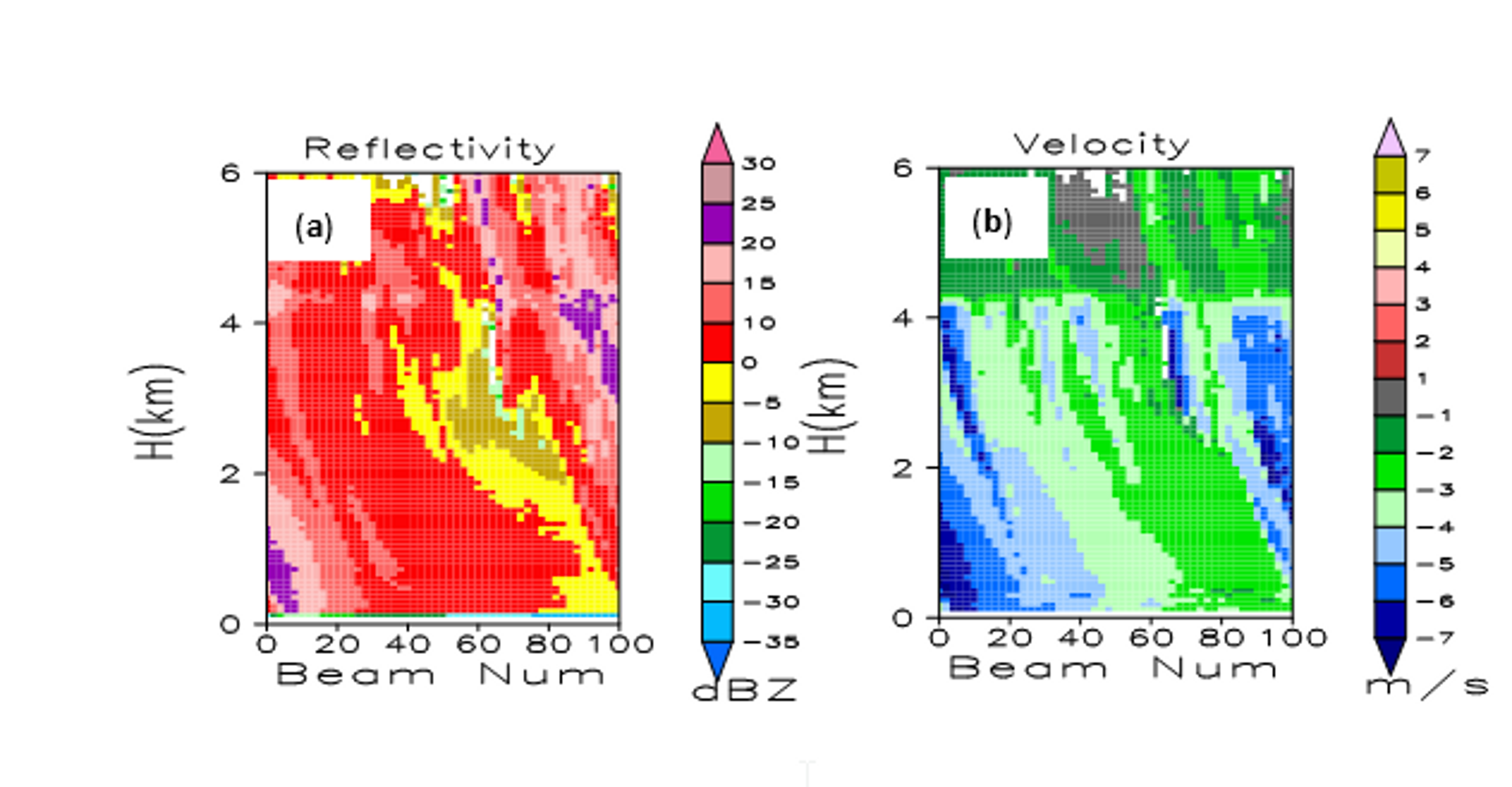
3.1. Consistency Analysis of Reflectivity and Velocity for the Four Modes and QC Results

Figure 1 shows time–height cross sections of 400 profiles of raw reflectivity and radial velocity measurements obtained using the M1 and M3 modes from 09:26 to 11:12 CST on May 21, 2018. Because the M1 mode does not perform pulse compression and coherent integration, data from this mode are the least affected. Hence, we compared results for the other three modes with those for the M1 mode. The M1 and M3 modes captured similar reflectivity and velocity values above the bright band at 4.5 km, with low velocity values under −2.0 m s−1. Below this altitude, velocity increased downward. Here, the M1 mode velocity was negative because of falling precipitation particles. A large proportion of these negative velocities exceeded the M3 Nyquist velocity of 5.7 m s−1. Note that parts of M3 velocity were positive, indicating aliasing of the radial velocity. The three rounds of coherent integration conducted in M3 resulted in a negative bias in reflectivity below the bright band when radial velocity exceeded 4 m s−1. That is, the full gain of coherent integration was not applicable for a large Doppler velocity, which led to radar returns that rapidly decorrelated over time.
To explain contamination from range sidelobe artifacts on the three moments of Doppler spectra and evaluate QC results, we conducted Doppler spectra density QC to remove velocity aliasing and range sidelobe artifacts, merged the Doppler spectra, corrected attenuation, and then merged the spectra and recalculated the three moments of Doppler spectra. Figure 1e,f show recalculated radial velocity and spectrum width after dealiasing, and Figure 1g and h show the corresponding results obtained after dealiasing and artifact removal for M3. The dealiasing Doppler spectral density algorithm recovered negative velocity in M3 similar to that in M1. The pulse compression sidelobe produced a band with a larger spectrum width above the bright band, marked by a red arrow in Figure 1f, and an artifact indicated by red circles in Figure 1c,d. Doppler spectra QC successfully removed these contaminants.
Figure 2 shows recalculated reflectivity, velocity, and spectral width from merged Doppler spectral density. To analyze the attenuation correction effects of reflectivity spectral density on reflectivity, we also show the reflectivity before attenuation correction in Figure 2a. The algorithm resolved underestimated reflectivity caused by coherent integration in M3 (Figure 1c) and resolved range sidelobe artifact contamination on spectral width over the bright band (Figure 1f) and correction attenuation. Attenuation correction increased reflectivity.
To compare reflectivity attenuation coefficients calculated from the retrieved DSD with that from the conventional K–Z relationship, we also calculated attenuation coefficients using Wang’s algorithm [25]. In this work, the K-Z relationship for 8.6 mm wavelength was obtained under the assumption that the DSD follow the Gamma distribution by sampling them 1330 times:
N ( D ) = C 1 D μ exp [ ( 3 . 67 + μ ) D / D 0 ]
where 0.00015 < C1 < 0.15, −1 < μ < 4, 0.15 mm < D0 < 1.0 mm.
Attenuation coefficients for drizzle liquid precipitation can be expressed as:
K Z = 0 . 00087 Z 0.93
where KZ is the attenuation coefficient (dB km−1) and Z is reflectivity (mm6 m−3). The attenuation coefficients from retrieved DSD is calculated by using Equation (1). Figure 3 shows a comparison between the attenuation coefficients from the retrieved DSD and the K–Z relationship. Z is probably in proportion to D6 and K is in proportion to D3. The DSD algorithm produced attenuation coefficients nearly two times larger than those produced by the Z–K relationship. This was possibly due to retrieved DSD in observation site in Hebei Province consisting mostly of large drops and the simulated DSD in the K–Z relationship being mostly composed of small drops, because the K-Z relationship in Equation (7) is suitable for drizzle. The differences between two kinds of attenuation coefficients depend on the parameters of DSD, which introduce an attenuation correction error.

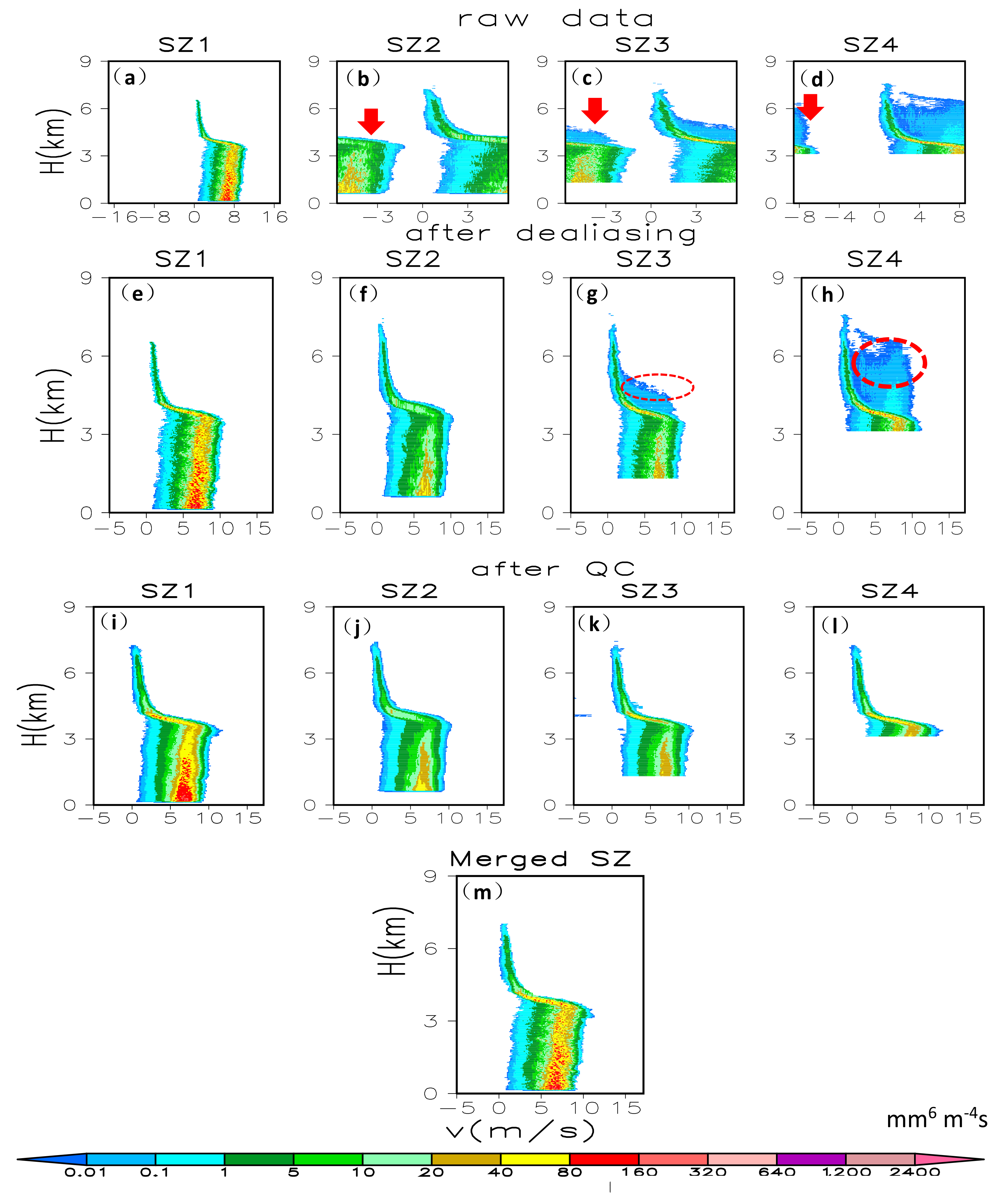
3.2. Consistency Analysis of Doppler Spectral Density for the Four Modes and Merged Results

Figure 4 shows raw Doppler spectra density data and data after dealiasing and artifact removal for the 30th profile. In Doppler spectral density data, positive velocities are downward. The Doppler spectra for solid precipitation above 4.5 km were narrow. In the bright band (4.0–4.5 km), solid hydrometeor spectra were widened by the melting process, resulting in wrapped aliased Doppler spectra SZ2, SZ3, and SZ4 for liquid hydrometeors. For SZ3 and SZ4, range sidelobes for larger Doppler velocities produced by liquid hydrometers appeared between 4.5 and 6.5 km. Operational modes M2, M3, and M4 underestimated reflectivity spectra for Doppler velocities > 3 m s−1. Comparing raw (Figure 4b–d) and QC data (Figure 4f–l) shows that aliasing for SZ2, SZ3, and SZ4 below 4 km were addressed correctly, the artifacts for solid hydrometeors in SZ3 and SZ4 were removed, and Doppler spectra from solid hydrometeors were preserved. Using the Doppler spectra, we not only removed artifacts in the SZ3 and SZ4 bins but also retained uncontaminated bins that were used to correct and recalculate reflectivity, velocity, and spectral width. However, using reflectivity instead of Doppler spectral density data would make it difficult to remove artifacts.
An important issue in all four operational modes is attenuation of the return power through the coherent integration circuitry [1]. The ratios of reflectivity and Doppler spectra from operational modes M2, M3, and M4 compared with M1 as a function of velocity, are shown in Figure 5. The reflectivity of any collection of hydrometeors with radial velocity exceeding approximately 2 m/s in a radar sample volume will be underestimated when using coherent integration in the M2, M3, and M4 operational modes. A similar situation occurs with Doppler spectra density, where Doppler spectra density underestimation is not negligible for velocities exceeding approximately 4 m/s. A reflectivity underestimation of −2 dB for operational modes M2 and M3, which have three times of coherent integration, responds to the 4 and 7 m/s fall speeds for M4, which has two instances of coherent integration. For the Doppler spectra, this situation occurs when velocities are 5 m/s for M2 and M3 and 8 m/s for M4, respectively. The gains of three and two coherent integrations are 4.7 and 3.0 dB, respectively, which indicates that coherent integration does not have any positive effects on reflectivity observations when fall speeds exceed approximately 6 and 8 m/s for M2, M3, and M4, respectively.

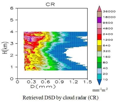
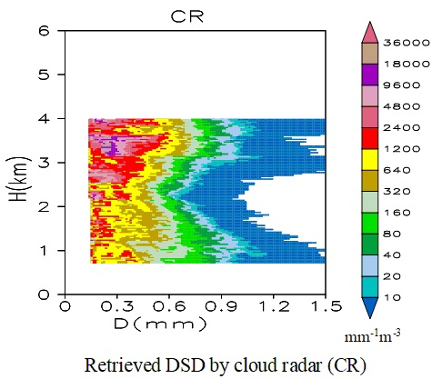
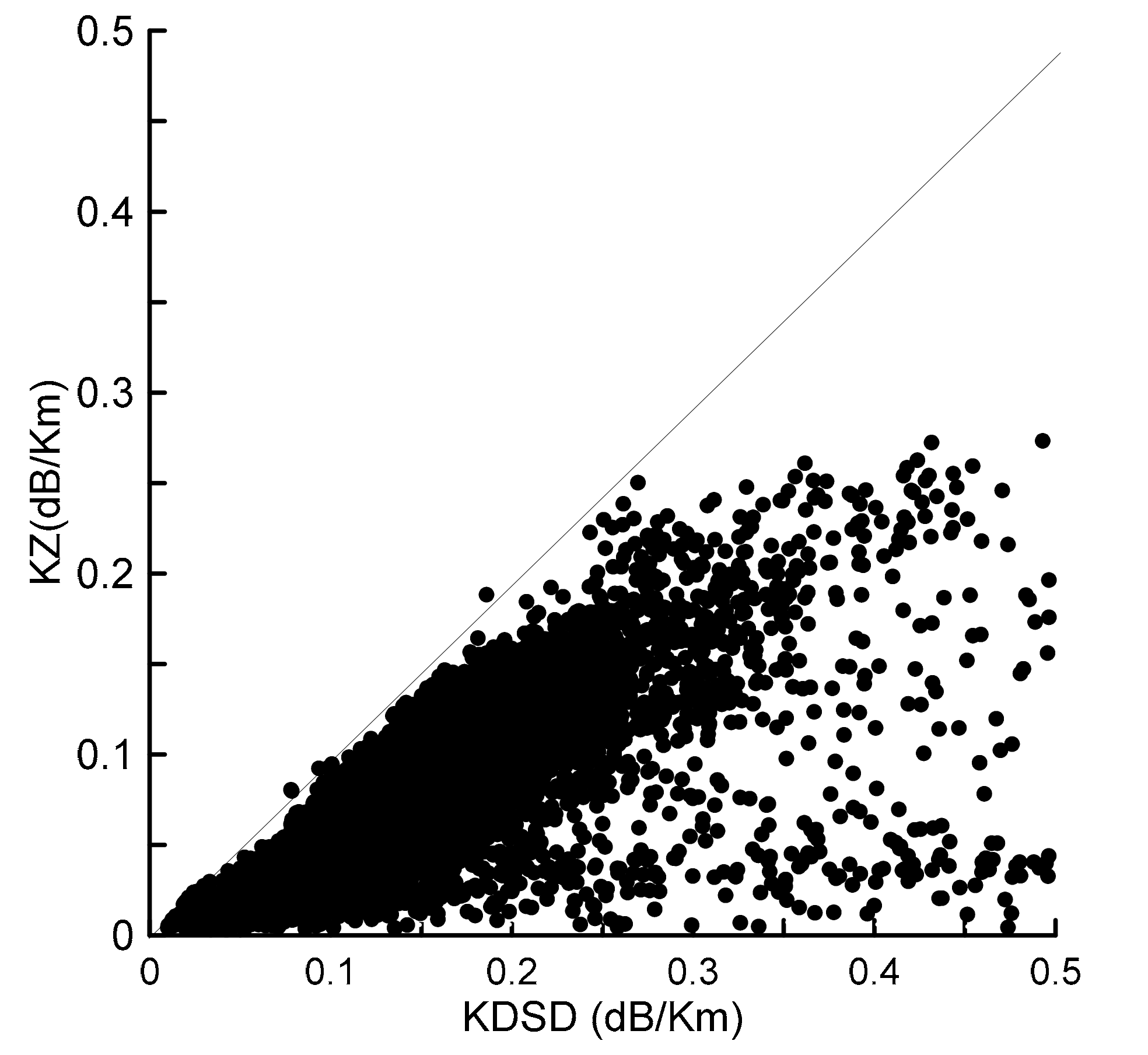
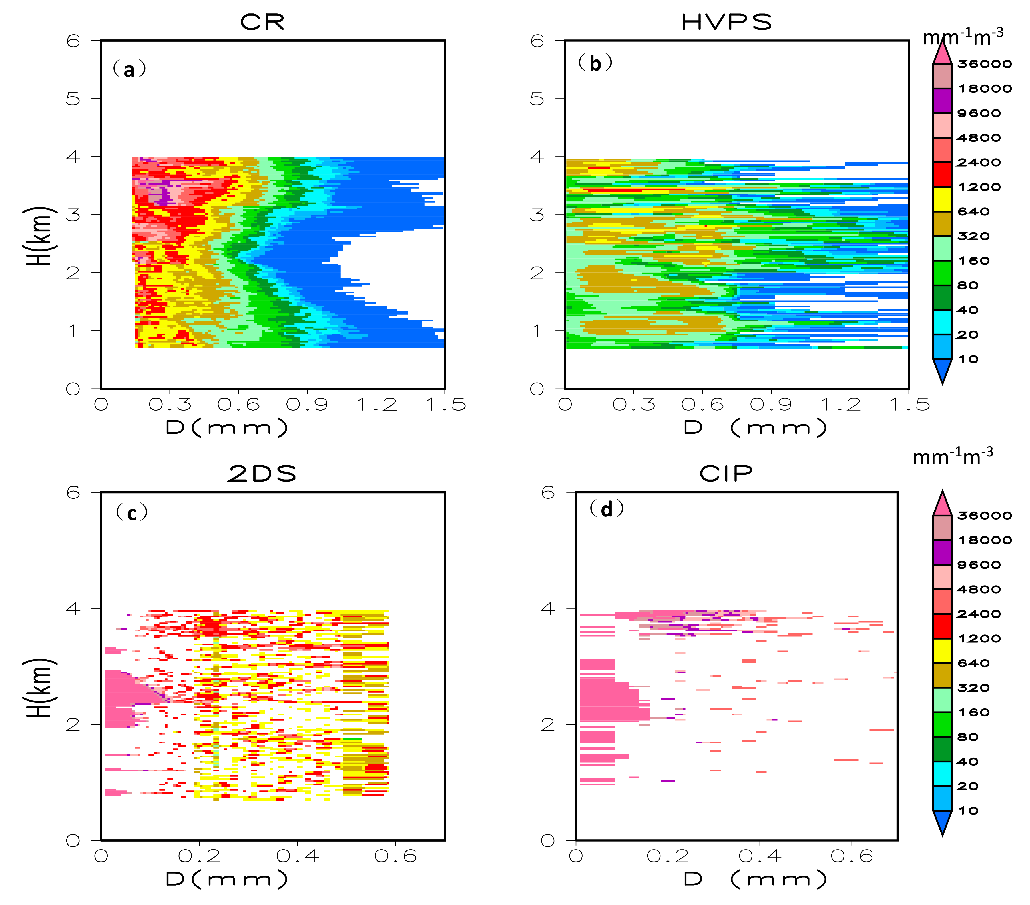
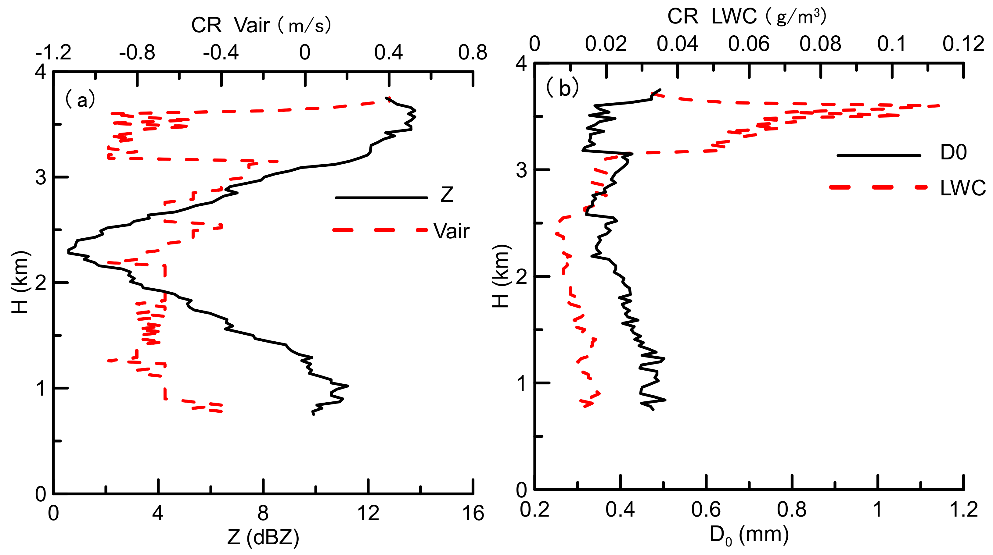
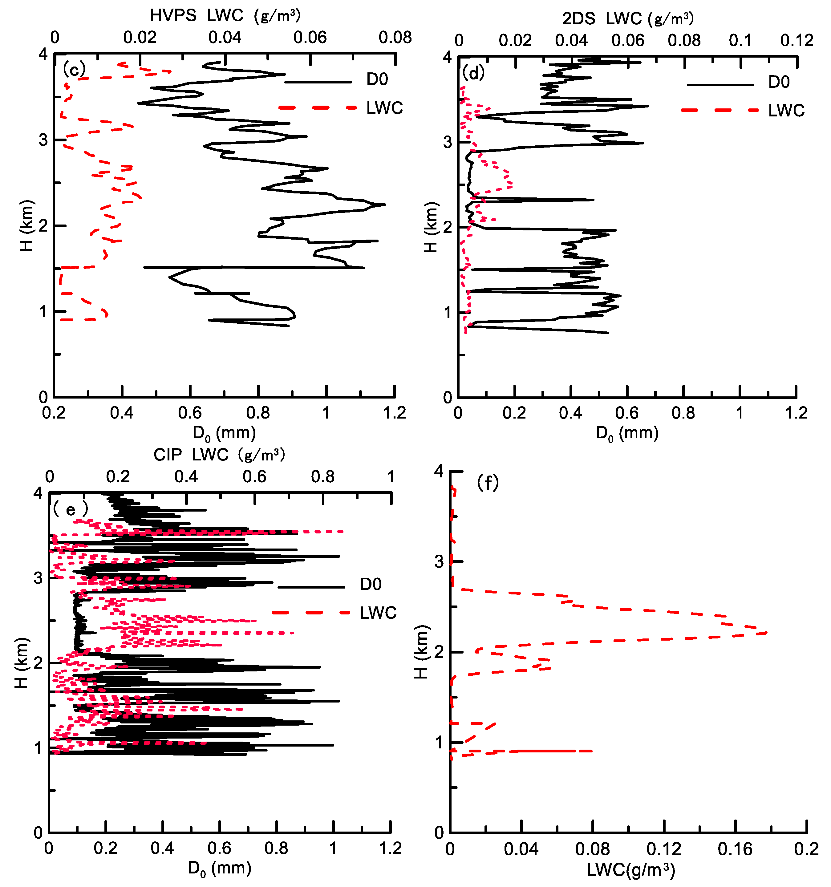
3.3. Application of CR Data to Microphysical Parameter Analysis

Stable stratiform precipitation occurred in Hebei Province in May 21, 2018. The CR observed cloud and precipitation vertical structures for the whole day, and the aircraft performed in situ observations over the station from 13:17 to 13:49 CST between 700 and 4900 m. Figure 6 shows time–height cross sections of recalculated reflectivity, velocity from merged Doppler spectra, retrieved vertical air speed, and hydrometeor fall speed. Figure 7 shows normalized contoured frequency by altitude diagrams of recalculated reflectivity, vertical air speed, and hydrometeor fall speed.
To analyze the attenuation correction, reflectivity before and after attenuation correction are both shown in Figure 6 and Figure 7. Maximum reflectivity reached 25 dBZ, and echo tops reached 11 km, with relatively heavy precipitation occurring during 08:00–16:00 CST.
We observed variations in bright band altitude over time, with the bright band reaching its minimum and maximum values at 04:00 and 16:00 CST, respectively, with a variational extent of approximately 500 m. It is useful to note that attenuation in low liquid precipitation with reflectivity stronger than 25 dBZ has more obvious effects on echo tops. By comparing Figure 6a,b with Figure 7a,b, we can see that attenuation correction increases the reflectivity in high level and mitigates reduction of reflectivity with height.
The vertical air speed results show that there are weak downdrafts in regions of stratiform liquid precipitation due to precipitation’s drag action on air. At 16:30, a precipitation greater than 25 dBZ passed the observation station at a low level, with attenuation leading to an underestimation of the echo top. An updraft was observed near the heavy precipitation at 16:00, and weak updraft regions were observed in the solid and weak liquid precipitation.
To reduce air pressure effects on hydrometeor fall speed, hydrometeor speed is corrected to ground as follows:
V T 0 = V T   ρ ρ 0 0.4
ρ = ρ 0 e 0.104 h
where VT0 and VT are hydrometeor fall speeds at ground and altitude h and ρ and ρ0 are the corresponding air densities, respectively. For both raw and corrected hydrometeor fall speeds (Figure 6e,f and Figure 7d), we can see that solid hydrometeor fall speeds increase and liquid hydrometeor fall speeds decrease with decreasing height, meaning that solid hydrometeors became larger when falling. This trend reflects the downward growth of ice particles by aggregation of hydrometeors or by riming of supercooled cloud water in upper cloud layers. In contrast, liquid hydrometeors became small because of evaporation or big drops breaking. Figure 7a–c show that solid hydrometeor melting increases reflectivity by 12 dB and fall speed by 6 m/s.
Figure 8 shows a comparison of vertical DSD profiles retrieved by the CR and measured by HVPS, 2DS and CIP. Figure 9 shows vertical profiles of reflectivity, vertical air speed by CR, LWC and volume-averaged particle diameter D0 by CR, HVPS, CIP and 2DS, LWC by hotwire probe. The aircraft temperature profile and CR reflectivity indicate that the temperature reaches 0 at 4.7 km. Between 4.0 and 4.7 km, solid hydrometeors begin melting, which increases the fall velocity and extends the spectra. Solid particles are melted to liquid by 4.0 km. The hydrometeor above 4 km are mixed or solid precipitation, which scattering and fall velocities have complicate relationships with diameters. In this case, DSDs, LWC and D0 above 4.0 km were not retrieved.
2DS and CIP observed maximum cloud drop number are 3.23*1010 and 1.08*109 mm−1mm−3 between 2 km and 3.0 km, respectively. 2DS missed the DSD when N (D) is less than 156 mm−1mm−3, and CIP missed more data when N (D) < 2900 mm−1mm−3. Due to the Doppler spectra’ resolution, CR could not retrieve the DSD when D < 0.15 mm. Both CR and HVPS observe most raindrops being 0.3–0.9 mm below 4 km and larger drops then 1.0 mm are founded above 2.5 km. CR and the three probes caught the large N(D) being 0.15–0.6 mm at 2.5 km and 3.5 km. CR and 2DS observed similar DSD patterns for 0.15 mm < D < 0.6 mm, however, CR retrieved a larger number of small drops of 0.5 mm than HVPS. CIP observed large N(D) then HVPS and 2DS.
Weak downdrafts observed by the CR are possibly due to drag from rain drops and an inversion layer between 2.1 and 3.3 km (Figure 9a). Figure 9b–e show a comparison between the CR LWC and Do and the four probes in airplane. It is noted that the CR and HVPS only samples larger particles so the LWC will be lower because it misses the contribution of the small drops and the D0 will be larger because this is an average size ignoring small drops. For CIP and 2DS, the large LWC and small D0 between 1.9 km and 2.9 km are contributed to small drops. Both CR and HVPS observed similar patterns of LWC below 3 km. However, the D0 values obtained by HVPR were twice those observed by CR. CR retrieved small averaged D0 than HVPS in situ observation, probably due to more small drops being detected by the CR.
In comparison of D0 from 2DS and CIP with CR, the D0 are calculated for particles for D > 0.15 mm, the both of D0 from 2DS and CIP are about 0.5 mm, which are similar with that by CR.

4. Discussion

The LWC and D0 biases between CR and in situ introduced by spatial variation of reflectivity are discussed in this section. Between 13:17 and 13:49 CST, the aircraft reached a maximum altitude of 4900 m and circled downward around the CR observation site to 700 m. The aircraft’s descending circle diameter was 18 km. Vertical variations in microphysical parameters around the CR site were observed for approximately 32 min. To explain the biases of microphysical parameters retrieved by CR and those from in situ observation, we analyzed precipitation variation during the aircraft’s observation (Figure 10). During this period, reflectivity showed obvious variation, especially between 1.8 and 4.0 km. The space distance and different observational volume by the CR and in situ observation also introduced uncertainties in comparisons between CR and aircraft data.
The relationship between liquid hydrometeor terminal velocity and diameter yields a Doppler spectral resolution of 0.133 m/s in response to the smallest diameter of 0.15 mm and a retrieved diameter resolution of approximately 0.028 mm. If the vertical air motion error is 0.266 m/s (2 grid), the diameter error would be approximately 0.056 mm. The CR would not retrieve raindrops smaller than 0.15 mm, and the variation of minimum reflectivity with height and operational mode should introduce vertical air motion bias, producing the retrieved DSD bias. The numerical experiment was made to examine the effects of range and work modes of CR under the assumption that the DSD follow the Gamma distribution. The results show that for drizzle precipitation with reflectivity of 7.0 dBZ, comparison with height of 2 km, the air motion is underestimated by 0.6 m·s−1 at height of 8 km. Comparison with M4, M1 underestimated air motion by 1.0 m·s−1.

5. Conclusions

The CR and an instrument-equipped aircraft were used to collect cloud and precipitation data in the east side of Taihang Mountain in Hebei Province in 2018. Algorithms for QC and merging of Doppler spectral density data from the four operational modes were used to process CR data, and an algorithm for attenuation correction based on retrieved DSD from the merged Doppler spectral density data was used to correct attenuation for reflectivity spectral density. The four types of Doppler spectral density data were then merged after dealiasing Doppler velocity and removing range sidelobe artifacts. We evaluated the consistencies of reflectivity spectra from the four operational modes and compared DSD retrieved using the CR with aircraft in situ observations. The major conclusions are as follows:
The four operational modes observed similar reflectivity and velocity for clouds and low velocity solid hydrometeors; however, three instances of coherent integration led to underestimated reflectivity spectra for Doppler velocities exceeding 4 m s−1, thus causing a large negative bias in the reflectivity. Reflectivity spectra were underestimated for low signal-to-noise ratios in the low-sensitivity mode, meaning it is useful to use data from operational modes M2, M3, and M4 with clouds or solid precipitation. Coherent integration and pulse compression increase the CR’s sensitivity and velocity resolution; however, it produced aliased velocity and Doppler spectral data and range sidelobe artifacts.
QC successfully removed the range sidelobe artifacts and dealiased the velocity and Doppler spectral data, and merging reflectivity spectra mitigated the underestimation of Doppler spectral density and reflectivity with larger velocities due to coherent integration, which yielded a comprehensive and accurate depiction of most clouds and precipitation in the vertical column above the CR. Attenuation correction using retrieved DSD improved tendency of reflectivity to decrease with height in stratiform precipitation, mitigating the effects of coefficient variations in K–Z relationships for clouds and precipitation in attenuation correction.
Weak vertical updrafts were found in solid and weakly reflecting liquid precipitation at upper levels and near heavy low-level precipitation. Most of the weak downdrafts existed in relatively strong precipitation, due to drag caused by hydrometeor fall speed. Reflectivity decreases and hydrometeor fall speeds increase with increasing altitude.
When compared with HVPS, CR observed similar DSD for diameters larger than 0.33 mm and found greater LWC. Additionally, the CR retrieved more small raindrops (diameter less than 0.3 mm) than HVPS, which corresponds to 2DS and CIP data. Comparing microphysical parameters between the CR and airborne in situ observations contained uncertainty because of differences in observation period and space as well as temporal and spatial resolutions of the data. More cases should be analyzed to further evaluate the CR’s observation capabilities.

Author Contributions

Conceptualization and methodology, L.L.; Cloud radar data curation, D.H.; Airplane observation analysis, D.X.; Cloud radar observation, C.J. and S.T.

Funding

This research was funded by the National Natural Science Foundation of China (91837310 and 41875036) and Operational Technology Experiment and Demonstration Project for Hail Suppression and Precipitation Enhancement in the east side of Taihang Mountain (HBRYWCSY_2017_00).

Acknowledgments

The authors would like to thank the Huangsi Observation Station, Xingtai Meteorological Bureau, and Anhui Sun Create Electronics Co., Ltd., for the observation data and producing the cloud radar.

Conflicts of Interest

The authors declare no conflicts of interest.

References

  1. Schmidt, G.; Ruster, R.; Czechowsky, P. Complementary code and digital filtering for detection of weak VHF radar signals from the mesosphere. IEEE Trans. Geosci. Electron. 1979, 17, 154–161. [Google Scholar] [CrossRef]
  2. Moran, K.P.; Martner, B.E.; Post, M.J.; Kropfli, R.A.; Welsh, D.C.; Widener, K.B. An unattended cloud-profiling radar for use in climate research. Bull. Am. Meteorol. Soc. 1998, 79, 443–455. [Google Scholar] [CrossRef]
  3. Clothiaux, E.E.; Moran, K.P.; Martner, B.E.; Ackerman, T.P.; Mace, G.G.; Uttal, T.; Mather, J.H.; Widener, K.B.; Miller, M.A.; Rodriguez, D.J. The Atmospheric Radiation Measurement Program Cloud Radars: Operational Modes. J. Atmos. Ocean. Technol. 1999, 16, 819–827. [Google Scholar] [CrossRef] [Green Version]
  4. Kollias, P.; Clothiaus, E.E.; Miller, M.A.; Luke, E.P.; Johnson, K.L.; Moran, K.P.; Widener, K.B.; Albrecht, B.A. The atmospheric radiation measurement program cloud profiling radars: Second-generation sampling stratrgies, processing and cloud data products. J. Atmos. Ocean. Technol. 2007, 24, 1119–1214. [Google Scholar] [CrossRef]
  5. Rogers, R.R. An extension of the Z-R relation for Doppler radar. In Proceedings of the 11th Weather Radar Conference, Boulder, CO, USA, 14–18 September 1964; pp. 158–161. [Google Scholar]
  6. Hauser, D.; Amayenc, P. A New Method for Deducing Hydrometeor-Size Distributions and Vertical Air Motions from Doppler Radar Measurements at Vertical Incidence. J. Appl. Meteorol. 1981, 20, 547–555. [Google Scholar] [CrossRef] [Green Version]
  7. Zheng, J.; Liu, L.; Zhu, K.; Wu, J.; Wang, B. A Method for Retrieving Vertical Air Velocities in Convective Clouds over the Tibetan Plateau from TIPEX-III Cloud Radar Doppler Spectra. Remote Sens. 2017, 9, 964. [Google Scholar] [CrossRef]
  8. Lhermitte, R. Observations of rain at vertical incidence with a 94 GHz Doppler radar: An insight of Mie scattering. Geophys. Res. Lett. 1988, 15, 1125–1128. [Google Scholar] [CrossRef]
  9. Kollias, P.; Albrecht, B.A.; Marks, F.D., Jr. Cloud radar observations of vertical drafts and microphysics in convective rain. J. Geophys. Res. 2003, 108, 40–53. [Google Scholar] [CrossRef]
  10. Gossard, E.E.; Strauch, R.G. Measurement of cloud droplet size spectra by Doppler radar. J. Atmos. Ocean. Technol. 1994, 11, 712–726. [Google Scholar] [CrossRef]
  11. Kollias, P.; Albrecht, B.A.; Lhermitte, R.; Savtchenko, A. Radar observations of updrafts, downdrafts, and turbulence in fair weather cumuli. J. Atmos. Sci. 2001, 58, 1750–1766. [Google Scholar] [CrossRef]
  12. Shupe, M.D.; Kollias, P.; Matrosov, S.Y.; Schneider, T.L. Deriving mixed-phase cloud properties from Doppler radar spectra. J. Atmos. Ocean. Technol. 2004, 21, 660–670. [Google Scholar] [CrossRef]
  13. Shupe, M.D.; Koliias, P.; Matrosov, M.; Eloranta, E. On deriving vertical air motions from cloud radar Doppler spectra. J. Atmos. Ocean. Technol. 2008, 25, 547–557. [Google Scholar] [CrossRef]
  14. Kollias, P.; Albrecht B, A.; Marks, F. Why Mie? Accurate observations of vertical air velocities and raindrops using a cloud radar. Bull. Am. Meteorol. Soc. 2002, 83, 1471–1483. [Google Scholar] [CrossRef]
  15. Löffler-Mang, M.; Kunz, M.; Schmid, W. On the Performance of a low-cost K-band Doppler radar for quantitative rain measurements. J. Atmos. Ocean. Technol. 1999, 16, 379–387. [Google Scholar]
  16. Kollias, P.; Lhermitte, R.; Albrecht B., A. Vertical air motion and raindrop size distributions in convective systems using a 94 GHz radar. Geophys. Res. Lett. 1999, 26, 3109–3112. [Google Scholar] [CrossRef]
  17. Liu, L.; Xie, L.; Cui, Z. Examination and application of Doppler spectral density data in drop size distribution retrival in weak precipitation by cloud radar. Chin. J. Atmos. Sci. 2014, 38, 223–236. (In Chinese) [Google Scholar]
  18. Kollias, P.; Rémillard, J.; Luke, E.; Szyrmer, W. Cloud radar Doppler spectra in drizzling stratiform clouds: 1. Forward modeling and remote sensing applications. J. Geophys. Res. 2011, 116, D13201. [Google Scholar] [CrossRef] [Green Version]
  19. Maahn, M.; Kollias, P. Improved micro rain radar snow measurements using Doppler spectra post-processing. Atmos. Meas. Technol. 2012, 5, 2661–2673. [Google Scholar] [CrossRef]
  20. Liu, L.P.; Zheng, J.F.; Wu, J.Y. A Ka-band solid-state transmitter cloud radar and data merging algorithm for its measurements. Adv. Atmos. Sci. 2017, 34, 545–558. [Google Scholar] [CrossRef]
  21. Liu, L.; Jiafeng, Z. Algorithms for Doppler spectral density data quality control and merging for the Ka-Band solid-state transmitter cloud radar. Remote Sens. 2019, 11, 209. [Google Scholar] [CrossRef]
  22. Paul Lawson, R.; O’connor, D.; Zmarzly, P.; Weaver, K.; Baker, B.; Mo, Q.; Jonsson, H. The 2D-S (Stereo) probe: design and preliminary tests of a new airborne, high-speed, high-resolution particle imaging probe. J. Atmos. Ocean. Technol. 2006, 23, 1462–1477. [Google Scholar] [CrossRef]
  23. Doviak, R.J.; Zrnić, D.S. Doppler Radar and Weather Observations, 2nd ed.; Academic Press: Cambridge, MA, USA, 1993; p. 562. [Google Scholar]
  24. Barber, P.; Yeh, C. Scattering of electromagnetic wave by arbitrarily shaped dielectric bodies. Appl. Opt. 1975, 14, 2864–2872. [Google Scholar] [CrossRef] [PubMed]
  25. Wang, Z.; Teng, X.; Ji, L.; Zhao, F. A study of the relationship between the attenuation coefficient and radar reflectivity factor for spherical particles in clouds at millimeter wavelengths (in Chinese with English abstract). Acta Meteor. Sin. 2011, 69, 1020–1028. [Google Scholar]
Figure 1. Time–height cross sections of 400 profiles of raw reflectivity and radial velocity measurements obtained using M1 (a,b) and M3 modes (c,d). Recalculated radial velocity and spectrum width after dealiasing only (e,f) and after dealiasing and artifact removal (QC) from M3 (g,h) for from 09:26 to 11:12 CST on May 21, 2018.
Remotesensing 11 01595 g001aRemotesensing 11 01595 g001b
Figure 2. Recalculated reflectivity before (a) and after (b) attenuation correction, (c) radial velocity, and (d) spectrum width.
Remotesensing 11 01595 g002
Figure 3. Comparison between attenuation coefficients by the drop size distribution (DSD) algorithm and the K–Z relationship. KDSD is from the DSD algorithm and KZ is from the K–Z relationship.
Remotesensing 11 01595 g003
Figure 4. Raw reflectivity spectra across different heights for the 30th profile observed using operational modes (a) M1, (b) M2, (c) M3, and (d) M4, after dealiasing only (e–h) and QC data after dealiasing, artifact removal and attenuation correction (i–l). Merged data (m). The aliased parts of the reflectivity spectra are indicated by a red arrow, and range sidelobe artifacts are highlighted with red circles.
Remotesensing 11 01595 g004
Figure 5. Ratios of (a) reflectivity and (b) Doppler spectral density measured by operational modes M2, M3, and M3 with M1 as a function of radial velocity.
Remotesensing 11 01595 g005
Figure 6. Time–height cross sections for recalculated reflectivity (a) before and (b) after attenuation correction, (c) velocity, (d) vertical air speed, (e) hydrometeor fall speed, and (f) corrected speed to ground. The black rectangle in (a) represents the aircraft observation period.
Remotesensing 11 01595 g006aRemotesensing 11 01595 g006b
Figure 7. Normalized contoured frequency by altitude diagrams (%) of recalculated reflectivity (a) before and (b) after attenuation correction, (c) vertical air speed, and (d) corrected hydrometeor fall speed to ground on May 21, 2018.
Remotesensing 11 01595 g007
Figure 8. Retrieved drop size distribution (mm−1m−3) at 13:18 by cloud radar (CR) (a) and observed DSD with the HVPS (b), 2DS (c) and CIP (d) between 13:17 and 13:49 CST.
Remotesensing 11 01595 g008
Figure 9. Vertical profiles of Z and vertical air motion retrieved by cloud radar (CR) (a), D0 and liquid water content (LWC) by CR (b), HVPS (c), 2DS (d), CIP (e) and LWC by hotwire (f).
Remotesensing 11 01595 g009aRemotesensing 11 01595 g009b
Figure 10. Time–height cross sections of reflectivity (a) and velocity (b) between 13:18 and 13:45 in the black rectangle.
Remotesensing 11 01595 g010
Table 1. Major technical parameters for the Ka-band solid-state transmitter cloud radar.
OrderItemsTechnical Specifications
1Radar systemCoherent, pulsed Doppler, solid-state transmitter, pulse compression
2Radar frequency35.0 GHz (Ka-band)
3Beam width0.30°
4Pulse repeat frequency8000 Hz
5Peak power50 W
6Detecting parametersZ, Vr, Sw, LDR, SP
Detection capability≤−34.5 dBZ at 5 km
7Range of detectionHeight: 0.120–15 km
reflectivity: −45 to + 30 dBZ
radial velocity: −17.13 to 17.13 m s−1 (maximum)
velocity spectrum width: 0 to 4 m s−1 (maximum)
8Spatial and temporal resolutionsTemporal resolution: 16 s
Height resolution: 30 m
Notes: Z—reflectivity; Vr—radial velocity; Sw—spectrum width; LDR—linear depolarization ratio; SP—Doppler spectral density.
Table 2. Cloud radar subsystem parameters.
OrderItemsTechnical Specifications
Antenna Subsystem
1Operating frequencyKa-band
2Antenna gain≥53.6 dB
3Beam width≤0.30°
4First sidelobe level ≤−22 dB
5Sidelobe level≤−42 dB
6Cross-polarization isolation32.0 dB
7Radar transceiver feeder≤3 dB
Transmitter subsystem
1SystemSolid-state transmitter
2Peak power≥50 W
3Duty ratio≥10%
Receiver subsystem
1Noise figure≤5 dB
2Reflectivity dynamic range≥75 dB
3Phase noise≤−96 dBc/Hz at 1 kHz
4Intermediate frequency (IF) processingDigital IF receiver
The signal processing subsystem
1A/D bits≥14 bits
2Signal processingPulse compression, FFT, coherent integration, incoherent integration
3Range solution30 m
4Number of range gates≥500
5OutputDoppler spectral density data
Table 3. Major parameters for the four operational modes.
OrderItemPrecipitation Mode (M1)Boundary Mode (M2)Middle Level(M3)Cirrus Mode (M4)
1Pulse width0.2 μs2 μs8 μs20 μs
2Pulse repetition frequency8000 Hz8000 Hz8000 Hz8000 Hz
3Number of coherent integrations1332
4Number of incoherent integrations4444
5Number of fast Fourier transform256256256256
6Dwell time4 s4 s4 s4 s
7Range sample volume spacing30 m30 m30 m30 m
8Minimum range30 m300 m 1200 m3000 m
9Maximum range18 km18 km18 km18 km
10Nyquist velocity17.13 m·s−15.7 m·s−15.7 m·s−18.56 m·s−1
11Velocity resolution0.068 m·s−10.023 m·s−10.023 m·s−10.034 m·s−1
12Minimum detective reflectivity at 5 km−12.4 dBZ−26.9 dBZ−32.9 dBZ−34.9 dBZ

