Interference Mitigation for Synthetic Aperture Radar Based on Deep Residual Network
by
 ,
,
Weiwei Fan
1, 
Feng Zhou
1,*,
Mingliang Tao
2,
Xueru Bai
3,
Pengshuai Rong
1,
Shuang Yang
1 and
Tian Tian
1 1
Key Laboratory of Electronic Information Countermeasure and Simulation Technology of Ministry of Education, Xidian University, Xi’an 710071, China
2
School of Electronics and Information, Northwestern Polytechnical University, Xi'an 710072, China
3
National Laboratory of Radar Signal Processing, Xidian University, Xi’an 710071, China
*
Author to whom correspondence should be addressed.
Remote Sens. 2019, 11(14), 1654; https://0-doi-org.brum.beds.ac.uk/10.3390/rs11141654
Submission received: 21 June 2019
/
Revised: 7 July 2019
/
Accepted: 8 July 2019
/
Published: 11 July 2019
(This article belongs to the Special Issue Radio Frequency Interference (RFI) in Microwave Remote Sensing)
Abstract
:Radio Frequency Interference (RFI) is a key issue for Synthetic Aperture Radar (SAR) because it can seriously degrade the imaging quality, leading to the misinterpretation of the target scattering characteristics and hindering the subsequent image analysis. To address this issue, we present a narrow-band interference (NBI) and wide-band interference (WBI) mitigation algorithm based on deep residual network (ResNet). First, the short-time Fourier transform (STFT) is used to characterize the interference-corrupted echo in the time–frequency domain. Then, the interference detection model is built by a classical deep convolutional neural network (DCNN) framework to identify whether there is an interference component in the echo. Furthermore, the time–frequency feature of the target signal is extracted and reconstructed by utilizing the ResNet. Finally, the inverse time–frequency Fourier transform (ISTFT) is utilized to transform the time–frequency spectrum of the recovered signal into the time domain. The effectiveness of the interference mitigation algorithm is verified on the simulated and measured SAR data with strip mode and terrain observation by progressive scans (TOPS) mode. Moreover, in comparison with the notch filtering and the eigensubspace filtering, the proposed interference mitigation algorithm can improve the interference mitigation performance, while reducing the computation complexity.

1. Introduction
Synthetic Aperture Radar (SAR) has the advantages of full-time, all weather, long range, wide-swath, and high-resolution imaging, which plays a very important role in the fields of remote sensing, reconnaissance, space surveillance, and situational awareness [1,2,3,4,5,6,7]. However, the measured SAR data can be corrupted by other electronic systems in the frequency band, such as communication systems, radiolocation radars, television networks, and other military radiation sources. The low-energy Radio Frequency Interference (RFI) can potentially be partly mitigated thanks to the large coherent signal-processing gain in the SAR imaging algorithm, while strong RFI will remain in the focused SAR images. At the same time, the presence of strong RFI would yield inaccurate estimates of critical Doppler parameters (e.g., centroid and modulation rate), which would result in blurry and defocused SAR images. The presence of the haze-like RFI in SAR images buries interesting targets. Moreover, it seriously degrades the quality of the SAR image, reducing the accuracy of feature extraction and posing a hindrance to the SAR image interpretation [8,9,10]. Therefore, it is necessary to develop an effective RFI detection and mitigation method to reduce the effects of RFI on SAR imaging.
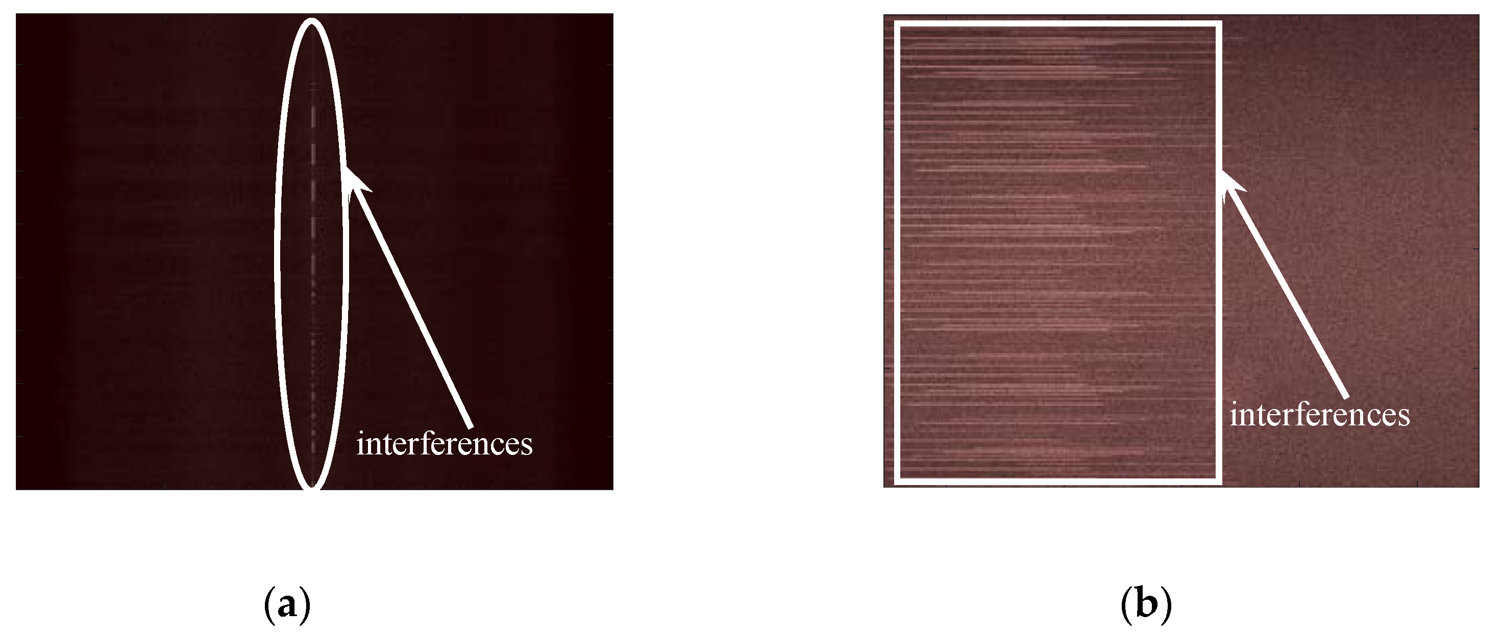
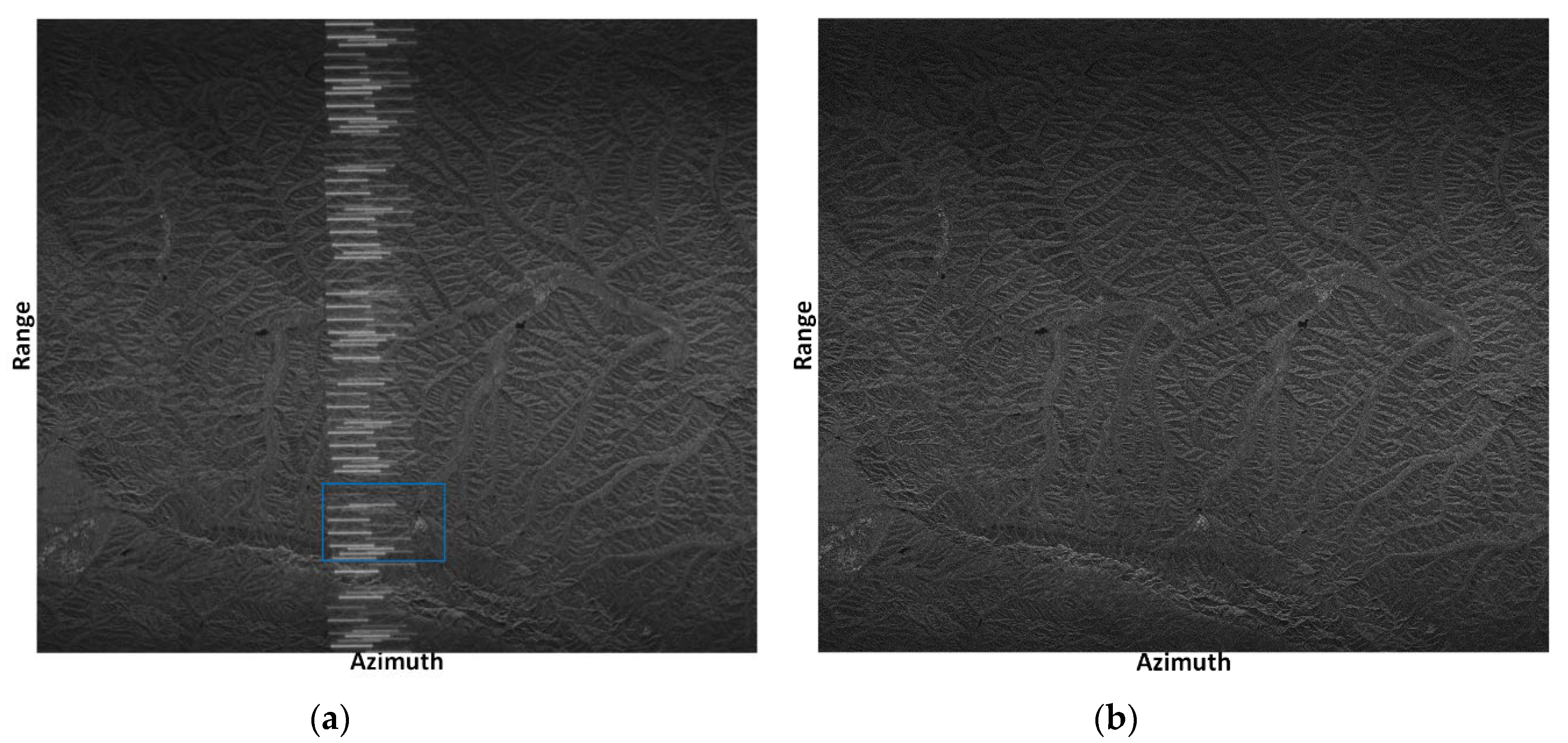
Generally speaking, RFI can be classified into two types, according to the relative bandwidth of the interference: narrow-band interference (NBI) and wide-band interference (WBI). Figure 1 shows the SAR echoes corrupted by NBI and WBI in two different domains to illuminate the difference between the interferences and useful target signals. Figure 1a shows the SAR echoes contaminated with NBI in the range-frequency azimuth-time domain. These echoes were collected in strip mode. The vertical bright line marked within the white ellipse is the NBI signal and the NBI occupies only a few frequency bins. Figure 1b shows the SAR echoes contaminated with WBI in the azimuth-frequency range-time domain. The echoes were acquired in the terrain observation by progressive scans (TOPS) mode. The bright lines marked within the white rectangle in Figure 1b represent the WBI with a wider bandwidth and the center frequencies vary randomly along the range time. It should be noted that the NBI and WBI can be represented in different domains. To better represent the interferences characteristics, the echoes corrupted by the NBI and WBI shown in Figure 1 are represented in the range-frequency azimuth-time domain and azimuth-frequency range-time domain, respectively.
Since NBI and WBI may be time-varying signals, not all of the SAR echoes contain interference. Therefore, it is necessary to identify whether interference exists in the SAR echoes. Zhou et al. developed an interference detection algorithm that assumed the amplitude of the useful target signal obeys the Gaussian distribution, while the interference-corrupted echo follows a non-Gaussian distribution [11]. Thus, the interference detection problem can be solved by measuring the deviation extent from the Gaussian distribution. In [11], kurtosis was adopted to evaluate deviation from the Gaussian distribution. Under the same principle, Tao et al. presented an interference detection method which utilized the negative entropy to measure the non-Gaussianity of the distribution [12]. The abovementioned interference detection algorithms can effectively identify whether there is interference in the SAR echoes. However, these two algorithms seriously depend on the threshold selection. If a higher threshold is selected, it will increase the missed-detection probability. If a lower threshold is chosen, the probability of false alarms will increase.
In the past few decades, various RFI mitigation methods have been developed to mitigate the influence of RFI on SAR imaging [11,12,13,14,15,16,17,18,19,20,21,22,23,24,25,26]. Generally, these interference mitigation algorithms can be divided into two types. The first are parametric methods, which mainly utilize mathematical models to characterize the SAR echoes and optimize the model parameters under specific criteria [15,16,17,18]. Then, the interference is reconstructed from the contaminated SAR echoes. Guo et al. developed an interference mitigation method based on the maximum a posterior (MAP) estimation and Bayesian inference [18]. After careful modeling of sparse prior and data likelihood, the method performs a Bayesian inference of the posterior and estimates the model parameters by MAP. Then, it reconstructs NBIs and subtracts it from the NBI-contaminated SAR echoes. However, parametric methods generally require high accuracy prior knowledge, and the model error will seriously restrict the interference mitigation performance.
The other type is nonparametric interference mitigation methods, which mainly design a reasonable filter and separate the interference and useful signal in a specific domain [11,12,13,14,19,20,21,22,23,24,25,26]. Range-spectrum notch filtering is a simple but efficient method for interference mitigation. It has been utilized in Advanced Land Observation Satellite (ALOS) Phased Array type L-band Synthetic Aperture Radar (PALSAR ) [8] and Experimental airborne Synthetic Aperture Radar (E-SAR) systems [19]. However, it fails at WBI mitigation because it introduces too much signal loss and distortion. Tao et al. investigated WBI mitigation methods for high-resolution airborne SAR [12]. In [12], the WBI-corrupted echoes were characterized in the time–frequency domain by utilizing the short-time Fourier transform (STFT). In this way, the original range-spectrum WBI mitigation problem can be simplified into a series of instantaneous spectrum NBI mitigation problems. Instantaneous spectrum notch filtering and eigensubspace filtering were utilized to perform this NBI mitigation. Instantaneous-spectrum notch filtering can achieve a tradeoff between accuracy and efficiency. The eigensubspace filtering can effectively mitigate the WBIs in the SAR echoes with less signal loss, but with a relatively larger computation burden.
Deep convolutional neural network (DCNN) can automatically extract the hierarchical features of the targets in the images, and have been successfully applied to image classification [27,28,29], target detection [30,31,32], semantic segmentation [33,34,35], noise suppression [36,37], image super-resolution [38], image fusion [39], image generation [40,41], and image transformation [42,43]. Simonyan et al. proposed a visual geometry group (VGG) network and investigated the effect of the convolutional network depth on the accuracy in the large-scale image recognition setting, which achieves state-of-the-art classification results on the Image Net Challenge 2014 [28]. Michelsanti et al. proposed a method to enhance the speech signal by utilizing the conditional Generative Adversarial Network (cGAN) [40], which uses the Pix2Pix framework to learn mapping from the spectrogram of noisy speech to an enhanced counterpart [37]. Ledig et al. presented a method for image super-resolution using GAN and the deep residual network (ResNet) [29], which can convert low-resolution images to high-resolution images and the generated images contain rich textural details [38]. Motivated by these advancements, we combine the ability of deep learning in feature extraction and image generation to identify whether the SAR echoes contain interference, and reconstruct the target signal from the interference-contaminated SAR echoes.
In this paper, we develop an interference detection and mitigation algorithm based on deep learning. Firstly, the interference detection network (IDN) is built, using the classical VGG network with 16 layers (VGG-16) [28] to identify whether the interference exists in the SAR echoes according to the difference between the useful target signal and the interference in the time–frequency domain. Then, ResNet and skip-connections are employed to extract the features of the useful target signal in the time–frequency domain and reconstruct the useful target signal. In this paper, the short-time Fourier transform (STFT) is utilized to characterize the SAR echoes in the time–frequency representation. Since the input of DCNN is a real-valued image, the complex-valued SAR echoes in the time–frequency domain need to be separated into the real part and the imaginary part. Finally, the inverse short-time Fourier transform (ISTFT) is utilized to transform the recovered echoes into the time domain. Moreover, the proposed interference mitigation network (IMN) based on ResNet can mitigate both NBI and WBI. Since the interference mitigation can be realized in parallel along range dimension or azimuth dimension, the time cost can be further reduced.
In summary, the contribution of this paper can be summarized as follows:
1) An interference detection algorithm based on DCNN is proposed, which can effectively extract the time–frequency characteristics of NBI and WBI. It outperforms the state-of-the-art approaches by using a classical convolutional neural network architecture of VGG-16;
2) An interference mitigation algorithm based on ResNet is proposed. Compared with the traditional interference mitigation, the IMN improves the NBI and WBI mitigation performance, while reducing the computational complexity. Moreover, the IMN can extract features of the useful target signal without designing a specific feature filter, which reduces the complexity of designing the interference mitigation algorithm.
The remainder of this paper is organized as follows. Section 2 introduces the time–frequency characteristics of the interference and interference detection method. Section 3 elaborates the interference mitigation algorithm based on ResNet. The experimental results and performance analysis of the interference mitigation on the simulated and measured data are presented in Section 4, followed by the discussion in Section 5 and conclusions in Section 6.
2. Interference Formulation and Detection
In this part, we analyze the interference in the time domain, frequency domain, and time–frequency domain. Then, we propose the interference detection method based on the DCNN.
2.1. Interference Formulation
For an SAR system, the received complex-valued SAR echo at fast time and slow time can be modeled by:
where , , and denote the useful target signal, the interference, and the additive noise, respectively. Interference can be classified into NBI and WBI according to the bandwidth of interference. The NBI can be written as:
where , , and denote the complex envelope, frequency, and phase of the th interference component, respectively. Generally, there are two ways to modulate WBI signal, the chirp-modulated (CM) WBI and sinusoidal-modulated (SM) WBI. The CM WBI signal can be expressed as:
where , , and are the complex envelope, frequency, and the chirp rate of the th interference component. Furthermore, the SM WBI signal can be defined as:
where , , , and denote the complex envelope, modulation factor, frequency, and initial phase of the th interference component.
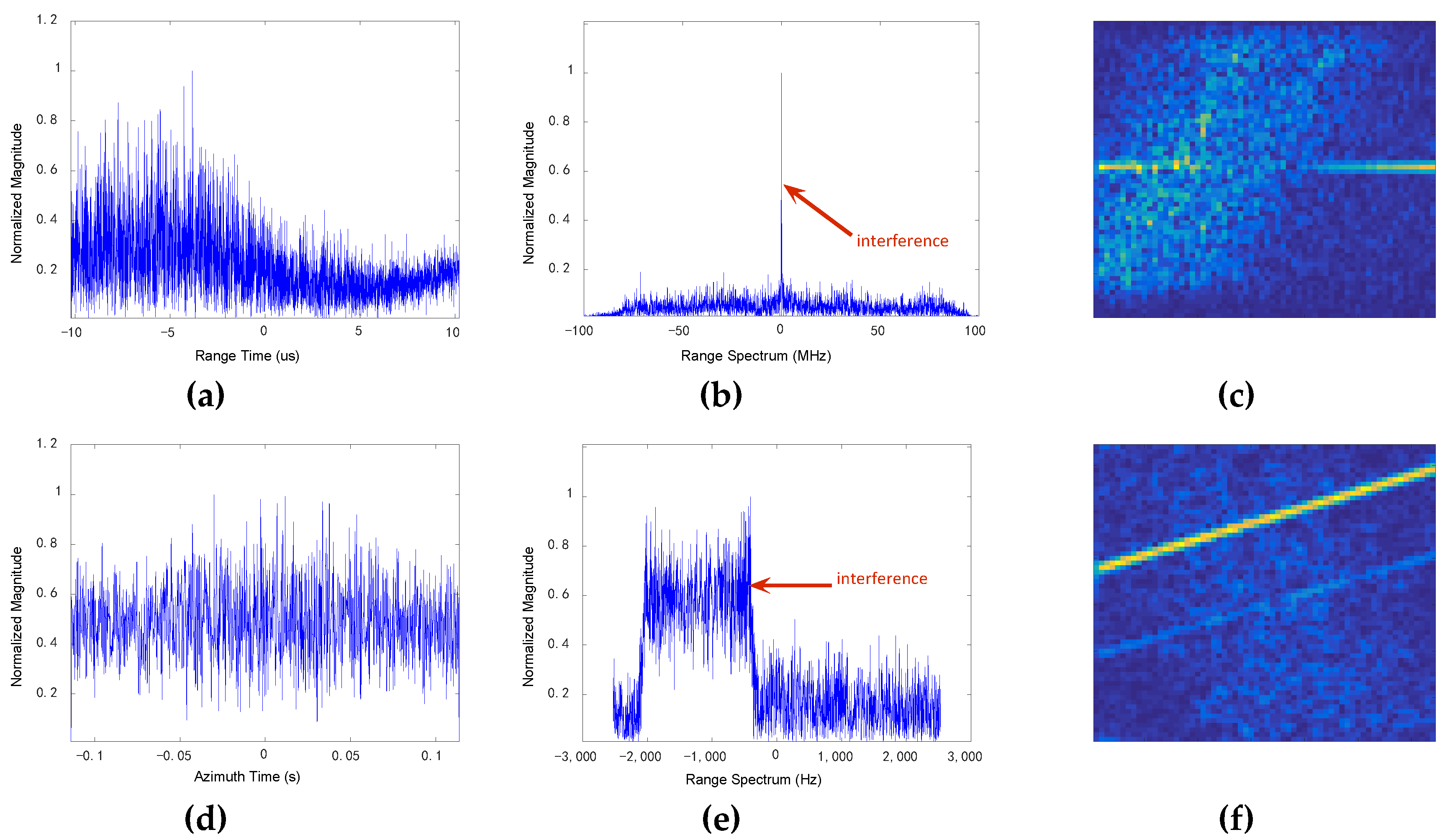
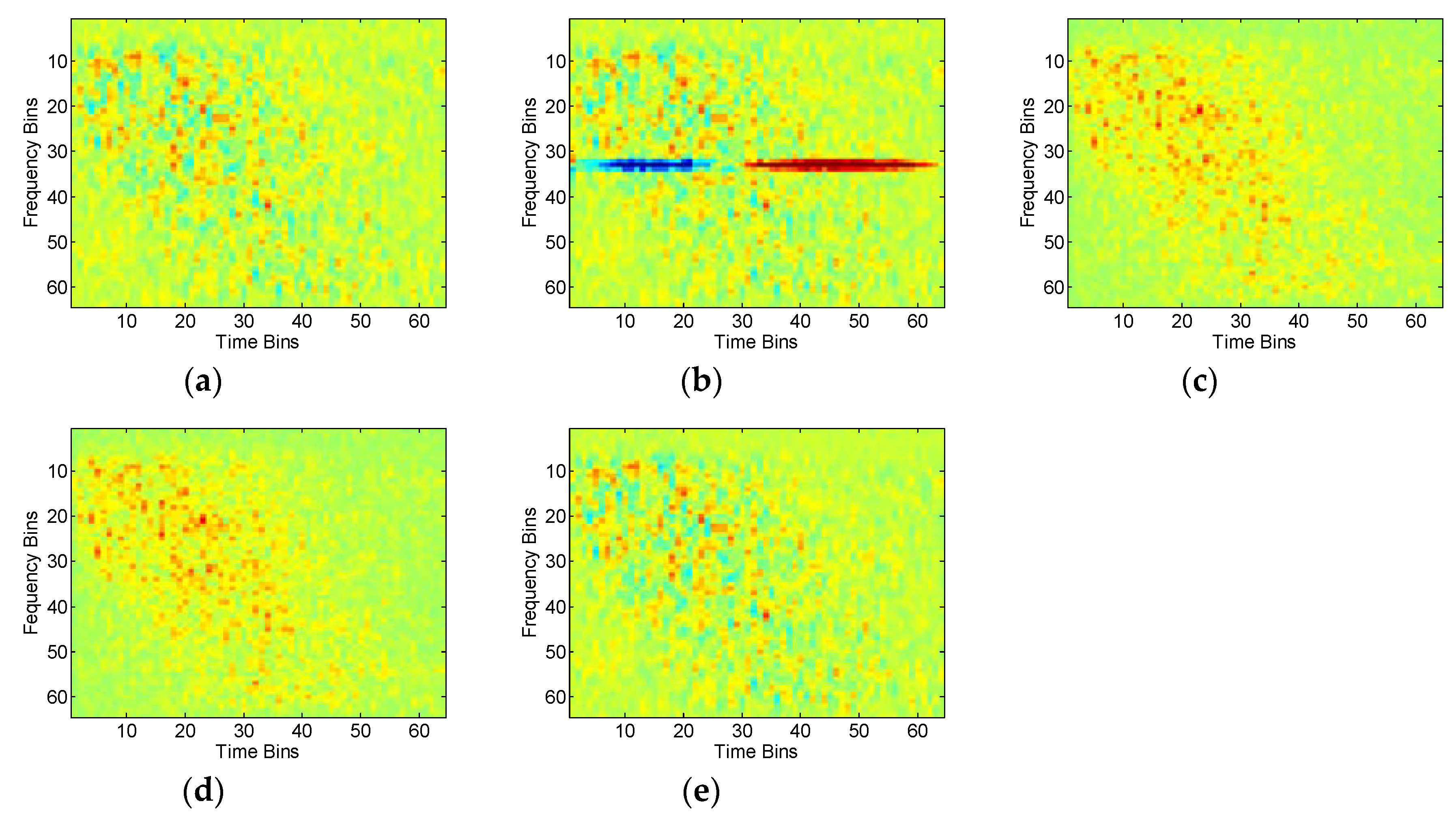
Figure 2 shows the interference-corrupted SAR echoes in different domains. The echo shown in Figure 2a–c is acquired from an airborne SAR system operating at X-band, and the echo shown in Figure 2d–f is collected from a space-borne SAR system operating at C-band. Figure 2a,d show that the echoes are contaminated by the NBI and WBI, respectively. The difference between the interference and the useful target signal is not obvious in the time domain. Figure 2b shows the range-spectrum of the NBI-corrupted echo. It is shown that the NBI energy mainly concentrates on a certain few frequency units and the amplitude of the NBI is much larger than the adjacent frequency units. Figure 2e shows the azimuth-spectrum of the WBI-corrupted echo, the WBI occupies a large proportion of bandwidth in the frequency domain and the amplitude of the WBI is stronger than the useful target signal. Figure 2c shows the time–frequency representation of the NBI-corrupted echo, the horizontal bright line is NBI and its amplitude is larger than surrounding useful target signal. Figure 2f shows the chirp modulated WBI-corrupted echo in the time–frequency domain, the line is the interference and its amplitude is much stronger than the surrounding useful target signal.
2.2. Interference Detection
An important step before applying the interference mitigation method is to identify whether the is interference in the SAR echoes. From Figure 2, it is difficult to determine the existence of interference in the time domain. However, the characteristics of interference are quite different for the useful target echo in the frequency domain and the time–frequency domain. Note that there are many interference detection methods in the frequency domain [11] and the time–frequency domain [12]. In this paper, we propose an IDN based on the DCNN which transforms the interference detection problem into a two-class classification problem. The IDN utilizes the VGG-16 architecture to capture the time–frequency characteristic divergence between the useful target signal and interference, and output the interference detection result. The VGG-16 consisted of 13 convolutional layers (Conv), 13 rectified linear units (ReLU), five maximum pooling layers (MP), three fully connected layers (Fc), and one softmax layer. Figure 3 shows a schematic diagram of the IDN based on VGG-16. The convolution kernel and stride of the Conv were set as and 1, respectively. The kernel and stride of the MP were set as and 2, respectively. Moreover, the specific structure of the IDN can be referred to in Table 1, and the third value in Conv denotes the number of feature maps.
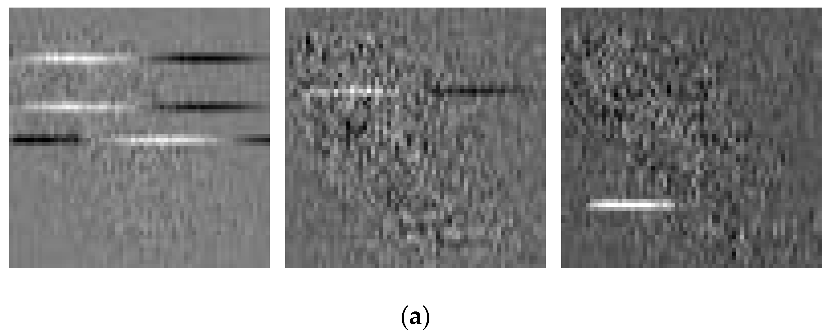
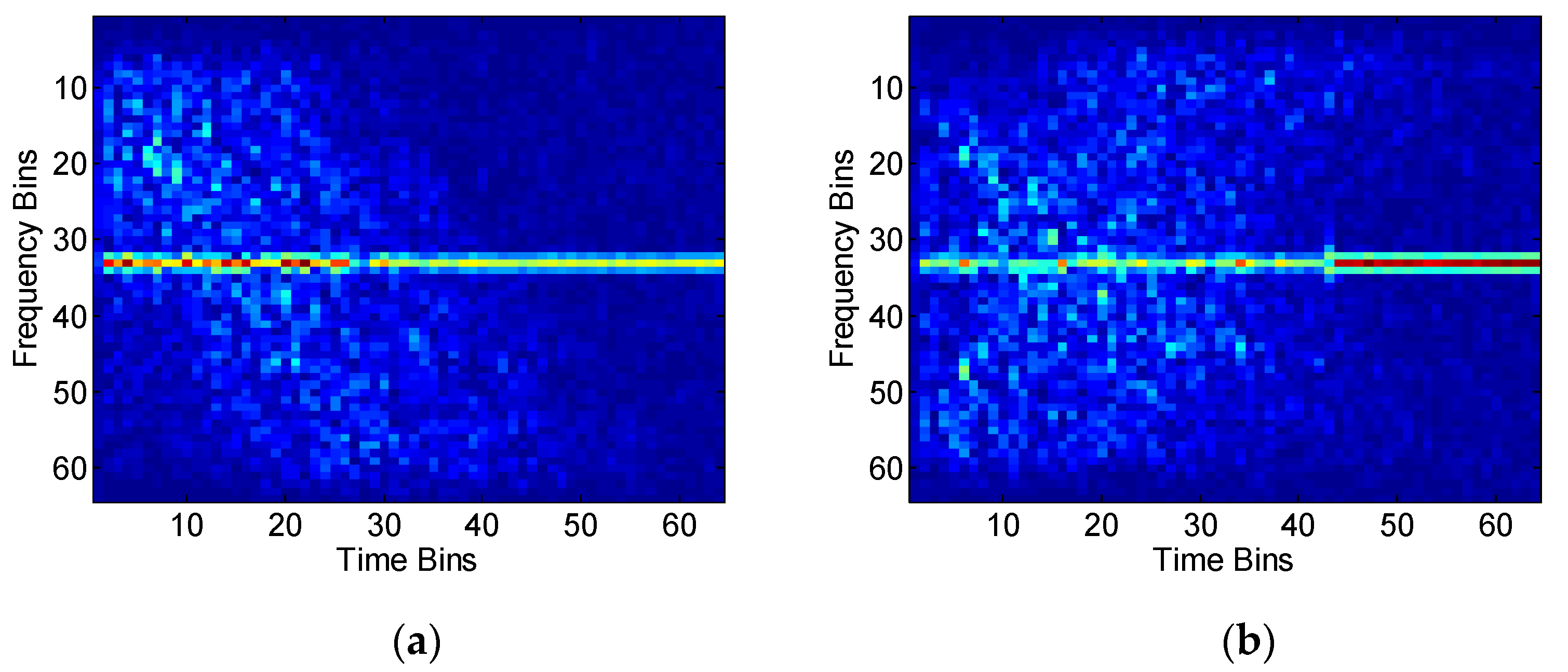
Figure 4 shows several training samples of different interference types in time–frequency representation by utilizing STFT. The training samples were classified into two categories. One was the useful target echo shown in Figure 4c, and the other was the interference-corrupted echo. The IDN should be capable of detecting NBI and WBI. Therefore, the interference-corrupted echoes consisted of the NBI-corrupted and WBI-corrupted echoes. Figure 4a,b show the samples of the NBI-corrupted echoes and WBI-corrupted echoes, respectively. Tensorflow [44] was utilized to train and test the IDN on the NVIDIA Titan-X Graphic Processing Unit (GPU). The Adam solver was utilized to optimize the network parameters [20]. The minimum batch size was set to 256, the first momentum was set as 0.5, the second momentum was set as 0.9, and the learning rate was set as 0.0001. Moreover, the weight parameter was initialized to a Gaussian distribution with a mean of 0 and a variance of 0.01, and the bias was initialized with a small constant of 0.1 [27].
To better illustrate the principle of IDN, we introduce the basics of a convolutional neural network.
2.2.1. Convolutional Layer
The convolutional layer is the core building block of a convolutional network, which can be interpreted as a set of learnable filters. Every filter is small spatially (along the width and height), but extends through the full depth of the input volume. During the forward pass, we slid each filter across the width and height of the input volume, producing a two-dimensional activation map. Stacking these activation maps for all filters along the depth dimension formed the full output volume. We defined the input feature maps of previous layers as , where is the number of feature units in the layer. The output feature maps were defined as , where is the number of feature units in the layer. Each unit in the convolution layer can be expressed as [27,28]:
where is ReLU; denotes unit of the activation map at position in layer; denotes the unit of the activation map at position in layer; denotes the trainable filter connecting the input feature map to the output feature map; denotes the trainable bias of the output feature map; every filter size is .
2.2.2. Pooling Layer
It is common to periodically insert a pooling layer between successive convolutional layers in the convolutional network architecture. It aims to progressively reduce the spatial size of the representation to reduce the number of parameters and computation in the network, to avoid overfitting. The pooling layer operates independently on every depth slice of the input and resizes it spatially, using max operation. The max pooling operation can be defined as [27,28]:
where is the pooling size; is the stride determining the intervals between neighbor pooling windows. The most common form is a pooling layer with filters of size applied with a stride of 2.
2.2.3. Softmax Classifier
The softmax classifier is utilized to solve the multiclass classification problems, which gives a slightly more intuitive output over each class and also has a probabilistic interpretation. The final output of the convolutional neural network is a k-dimensional vector, each element of which corresponds to the probability , for . The softmax nonlinearity operation can be calculated as:
where denotes the weighted sum of inputs to the unit on the output layer computed using (2). Given that training samples contain m components, it can be defined as , where denotes the true label of targets. Then, the lost function of cross-entropy can be expressed as [27,28]:
The cross-entropy loss function measures the difference between the correct label distribution and probability distribution estimated by the network. By minimizing this loss function, the trainable parameters will be adapted to increase the probability of the correct class label.
2.2.4. Back Propagation Algorithm
In DCNN, a back-propagation algorithm is utilized to compute the derivative of loss function with respect to trainable weights on each layer. In the back-propagation algorithm, we need to compute the error term, expressed as . The error term can be obtained by analytically computing derivation with respect to the parameter on each unit. For units in the output layer, the error term can be defined as:
where refers to the true label; and denotes the prediction of the convolutional network. Then, the previous layer error term can be computed through the output layer error term. If the layer is the convolutional layer, the layer error term can be defined as [27,28]:
where refers to the unit error term in the layer.
In the pooling layer, there are no trainable weights, but the error terms need to be back propagated to previous layers. If layer is max pooling layer, only the unit with the largest values are in the error term, while other units are defined as zeros. The error term in the layer can be defined as:
where denotes the Dirac delta function. After calculating the error term over each layer, the derivation of loss function respect to the convolution weights and biases can be expressed as:
3. Theory and Methodology
Here, we illustrate the training procedure and network architectures of the proposed IMN. Then, the metrics for evaluating performance are introduced.
3.1. Interference Mitigation Network
Compared with manual feature extraction and selection, DCNN can automatically capture the textural features and spatial information of the target in images. DCNN has wide applications in image generation, classification, detection, image segmentation, and image fusion. Motivated by the outstanding performance of DCNN in image processing, we developed the IMN for interference mitigation based on ResNet, the framework for which is shown in Figure 5. The IMN utilized the ResNet structure to solve the problem of network saturation and performance degradation when the structure of the IMN was deepened. The inputs and outputs of the IMN were interference-corrupted echoes and recovered echoes in the time–frequency representation, respectively. ResNet captured the features of the useful target signal and reconstructed the useful target signal in the time–frequency domain. The IMN consisted of 16 residual blocks, and was composed of two Conv, two batch normalization layers (BN), one ReLU, and one element-wise sum layer (Es). The kernel size and stride of Conv were set to be and 1, respectively. Moreover, the number of feature maps output by each Conv was 64. The detailed architecture of the IMN is shown in Table 2, where the residual block is denoted as Block.
The residual block connected the input and the output nodes through the structure of a skip-connection, so that the gradient of the previous layer could be directly passed to the output of the next layer. This could effectively solve the problem of gradient saturation at the deeper layers of the network. The optimization function of the residual network could be transformed into a residual function,
where is the input of the residual block; is the output of the th residual block; denotes the output of the though the Conv, BN, and ReLU. The loss function of the IMN was modeled by mean square error (MSE), which made the recovered echoes have a higher signal to noise ratio (SNR). MSE reflected the mean square error between the original signal without interference and the recovered signal. The loss function of the IMN based on MSE can be written as:
where and denote the width and height of the images, respectively; denotes the grayscale value of the original signal without interference in time–frequency domain at the point ; is the gray value of the recovered signal in time–frequency domain at the point by applying the IMN.
The complex-valued SAR echo was characterized in the time–frequency domain based on the STFT. To satisfy the requirements of the input for the IMN, the complex-valued SAR echo in the time–frequency domain was divided into real and imaginary parts. Then, the IMN was utilized to separately train on the real and imaginary parts. The IMN was trained on an NVIDIA Titan-X GPU using Tensorflow [44]. IMN utilized the Adam solver to optimize the network parameters [20]. The minimum batch size was set to 32, the first momentum was set as 0.5, the second momentum was set as 0.9, and the learning rate was set to 0.0001. Moreover, the weight parameter was initialized to a Gaussian distribution with mean 0 and a variance of 0.01, and the bias was initialized as a small constant 0.1 [38,45].
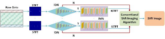
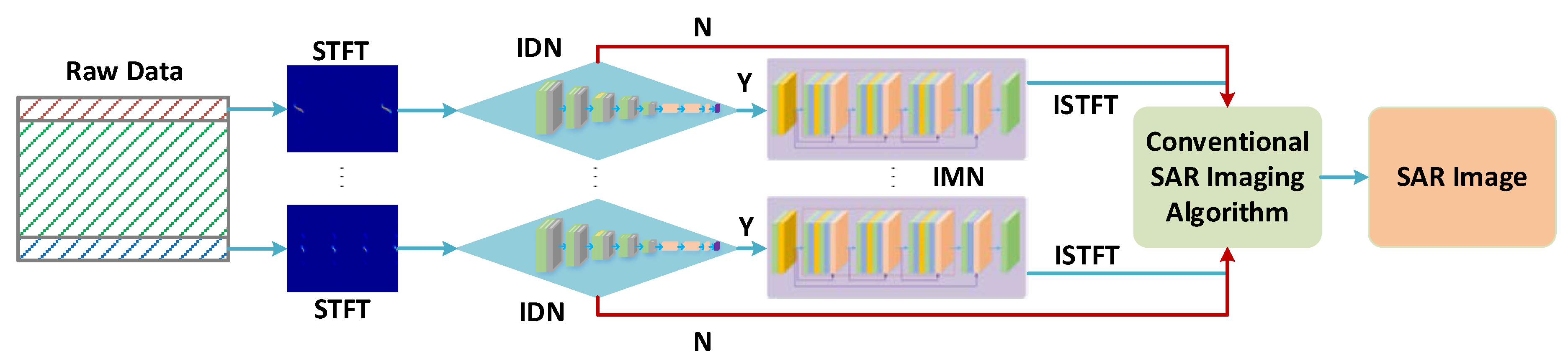
The workflow of the proposed scheme for interference detection and mitigation is shown in Figure 6. First, the STFT was applied to a single pulse along width range or azimuth to get a set of instantaneous spectra. For each spectrum, the DCNN-based interference detection method was carried out to identify whether there was interference in the echo. If the was interference, the IMN was performed to obtain a clean instantaneous spectrum. After parallel processing all of the instantaneous spectra, the clean instantaneous spectrum was returned to a time-domain signal by using the ISTFT. Then, conventional SAR imaging algorithms were utilized to generate SAR images.
3.2. Evaluation Measures
In order to verify the performance of the IMN, the performance of different interference mitigation algorithms was evaluated in a qualitative and quantitative way. For the qualitative evaluation, we visually compared the divergence of recovered signals and SAR imaging results by applying different interference mitigation algorithms. Moreover, we quantitatively evaluated the interference suppression ratio (ISR) [12], signal distortion ratio (SDR) [11], multiplicative noise ratio (MNR) [12], average gradient (AG) [46], mean square deviation (MSD) [39], and gray level difference (GLD) [47] performance over several test data.
3.2.1. ISR
ISR is defined as the ratio of the energy before interference mitigation to that after interference mitigation. This reflects the effect of interference suppression. The definition of ISR can be expressed as:
where denotes the interference-corrupted echo, and is the reconstructed signal after interference mitigation. A larger ISR value implies removing more interference from the received signal.
3.2.2. SDR
A large ISR may also indicate that the echo is seriously distorted. The SDR was introduced to evaluate the distortion of useful target signal after the interference mitigation. It is defined as the normalized energy loss of the useful target signal after the interference mitigation, which can be expressed as:
where denotes the original SAR echo without interference. A lower SDR means better useful target echo recovery with less distortion.
3.2.3. MNR
ISR and SDR are commonly adopted to evaluate the performance of interference mitigation on the simulated data. However, we could not obtain the ideal recovered echo in the measured data. Therefore, the MNR was introduced to evaluate the performance of the interference mitigation on the measurement data. MNR represents the average energy ratio of the weak scattering region to the adjacent strong scattering region in the SAR images. The definition of MNR can be expressed as:
where and indicate the number of pixels and the pixel values of the weak scattering region, respectively. Moreover, and denote the number of pixels and the pixel values of the strong scattering region, respectively. Smaller MNR means a better recovery of the system image response and better image contrast.
3.2.4. AG
The AG can reflect the presentation ability of image details and textures, which is always used to assess the SAR image sharpness [46]. For a given SAR image , the AG can be defined as:
where and denote the horizontal and vertical gradient values of the given SAR image , respectively. A larger AG implies clearer edge details of the image.
3.2.5. MSD
MSD is frequently used to measure the divergence between values predicted by a model, to evaluate the fluctuation of the gray value of image and the degree of focus of the image [39]. For a given SAR image , the MSD can be defined as:
where is the average gray value of the given SAR image. A larger MSD corresponds to a clearer image.
3.2.6. GLD
GLD not only considers the gray level changes of the transition region, but also represents the extent of the gray level changes, which can characterize the properties of transition region well [47]. For a given SAR image , the GLD can be defined as:
A larger GLD value implies that the image has clearer edge details.
We divided the evaluation measures into two categories. ISR and SDR were utilized to evaluate the interference mitigation performance for the simulated echoes. MNR, AG, MSD, and GLD were used to evaluate the SAR image quality after applying the interference mitigation algorithm. Meanwhile, a no-return area was needed in the scene to calculate the MNR.
4. Experimental Results
In this section, we conduct interference mitigation experiments on simulated and measured data to verify the effectiveness of IMN. Moreover, qualitative and quantitative metrics are utilized to evaluate the performance of different interference mitigation algorithms.
4.1. Results of the Simulated Data
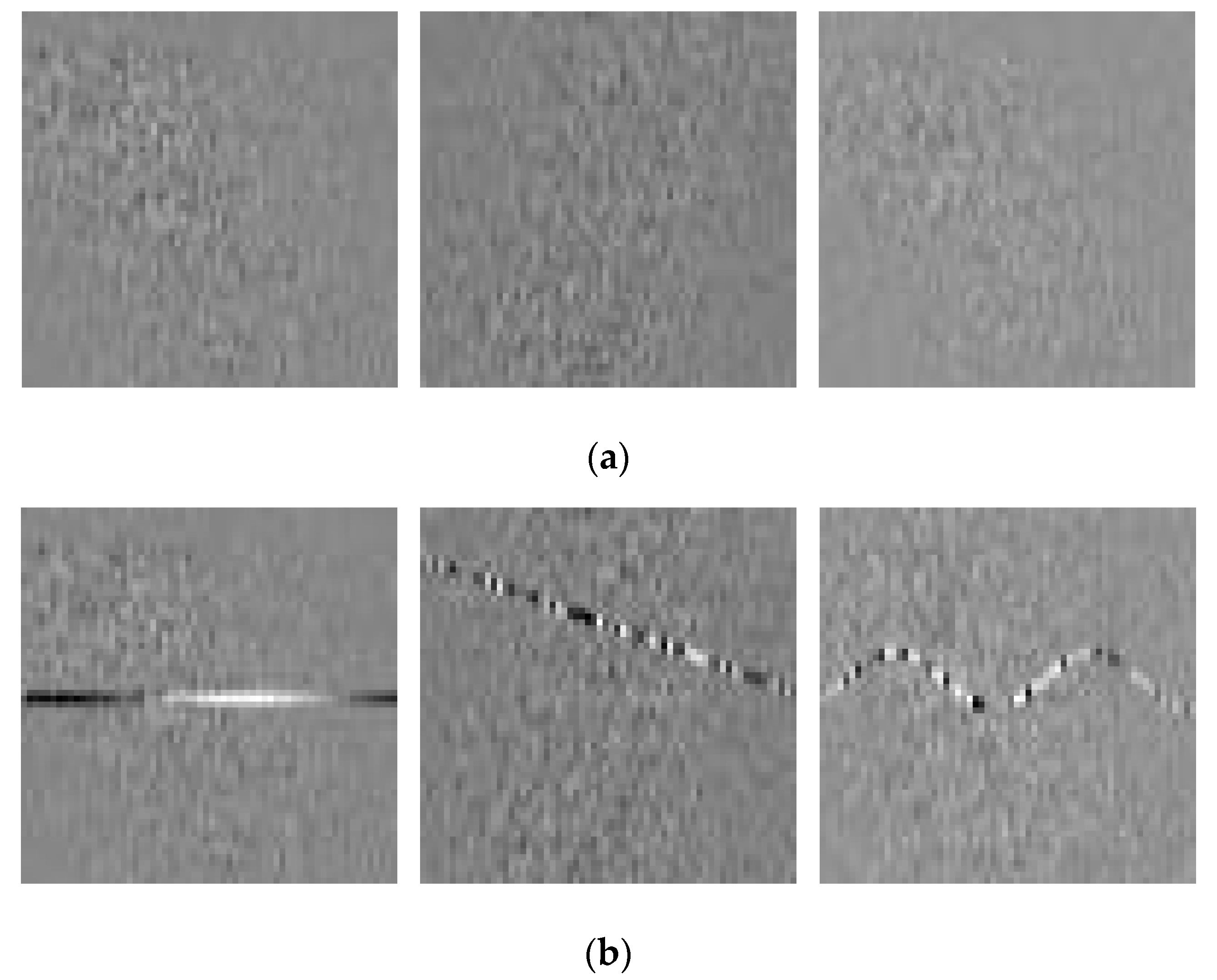
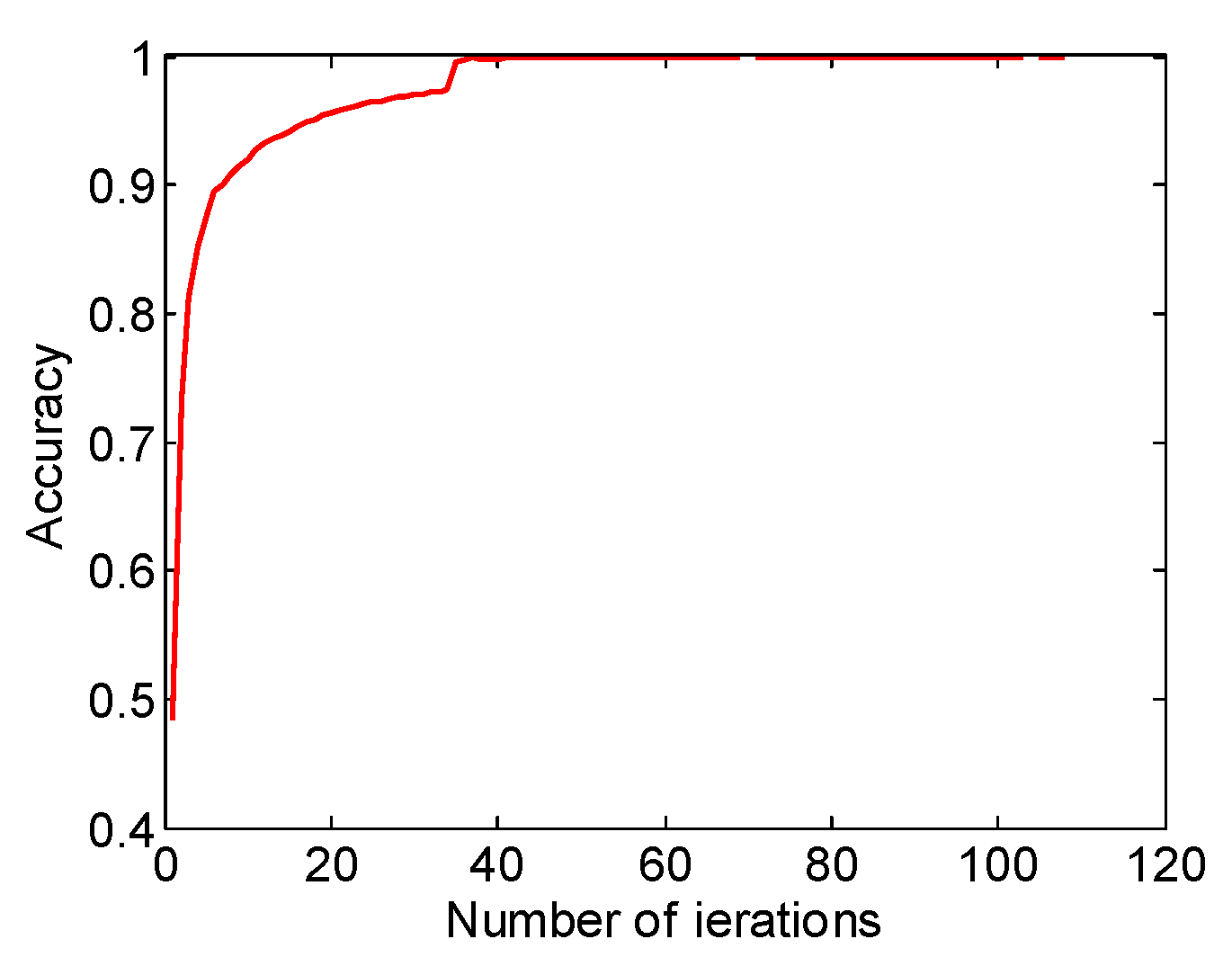
To validate the effectiveness of the IMN, we conducted interference mitigation experiments on the simulate NBI-corrupted and WBI-corrupted echoes. Figure 7a shows the original SAR echoes without interference in the time–frequency domain. The simulated NBI-corrupted and WBI-corrupted echoes in the time–frequency domain for training and testing the IMN are shown in Figure 7b. Before performing the IMN, the IDN was utilized to identify whether there was interference in the echoes. Figure 8 shows the convergence curve of training accuracy. It can be observed that the IDN accuracy gradually reached a stable 99.8%.
Figure 9a shows the STFT of the measured original NBI-free echo, while Figure 9b shows the STFT of the simulated NBI-contaminated echo. It can be seen that the existence of NBI significantly changes the spectrum of the useful signal, which severely hinders the interpretation of the embedded information. Figure 9c–e show the performance comparison of the range-spectrum notch filtering, the eigensubspace filtering, and the IMN, respectively. It can be seen that the original NBI-free echoes were recovered well via range-spectrum notch filtering and eigensubspace filtering, but also had less signal loss and distortion. Moreover, the echo recovered by applying the IMN was basically consistent with the original NBI-free echo, which illustrates the effectiveness of the IMN. To further illustrate the effectiveness of IMN, we utilized the ISR and SDR to evaluate the performance of the range-spectrum notch filtering, the eigensubspace filtering, and the proposed IMN, as shown in Table 3. The last column shows the improvement of the IMN compared with range-spectrum notch filtering and eigensubspace filtering. The proposed IMN had an overall good performance, with an improvement in the SDR, and obtained the highest ISR. This experiment demonstrates that the IMN achieves better NBI mitigation performance than the range-spectrum notch filtering and the eigensubspace filtering. It should be noted that only the ISR and SDR can be used to evaluate the performance of the interference mitigation for simulated echo.
Figure 10 compares the interference mitigation performance of the instantaneous-spectrum notch filtering, the eigensubspace filtering, and the IMN for the simulated WBI-contaminated echo. Figure 10a,b show the STFT of the original measured WBI-free echo and the WBI-contaminated echo, respectively. Figure 10c shows the interference mitigation result of applying the instantaneous-spectrum notch filtering method. Compared with Figure 10a, an obvious data gap can be observed in Figure 10c, which indicates severe signal loss. Figure 10d shows the result of applying eigensubspace filtering, which causes lower signal losses and distortion. Figure 10e shows that after applying the IMN, the recovered echo looks very similar to the original WBI-free echo. In order to further illustrate the effectiveness of IMN, the ISR and SDR were utilized to provide a quantitative performance comparison of the instantaneous-spectrum notch filtering, the eigensubspace filtering, and the IMN, as shown in Table 4. The last column of Table 4 shows the performance improvement of the proposed IMN. The three different methods achieved similar ISR, while generally the IMN performance was good, with an SDR improvement. It is shown that the IMN removes WBI and causes lower signal loss and distortion, which indicates that the IMN also achieves better interference mitigation than the WBI-corrupted SAR echo.
4.2. Results of the Measured NBI-Corrupted Data
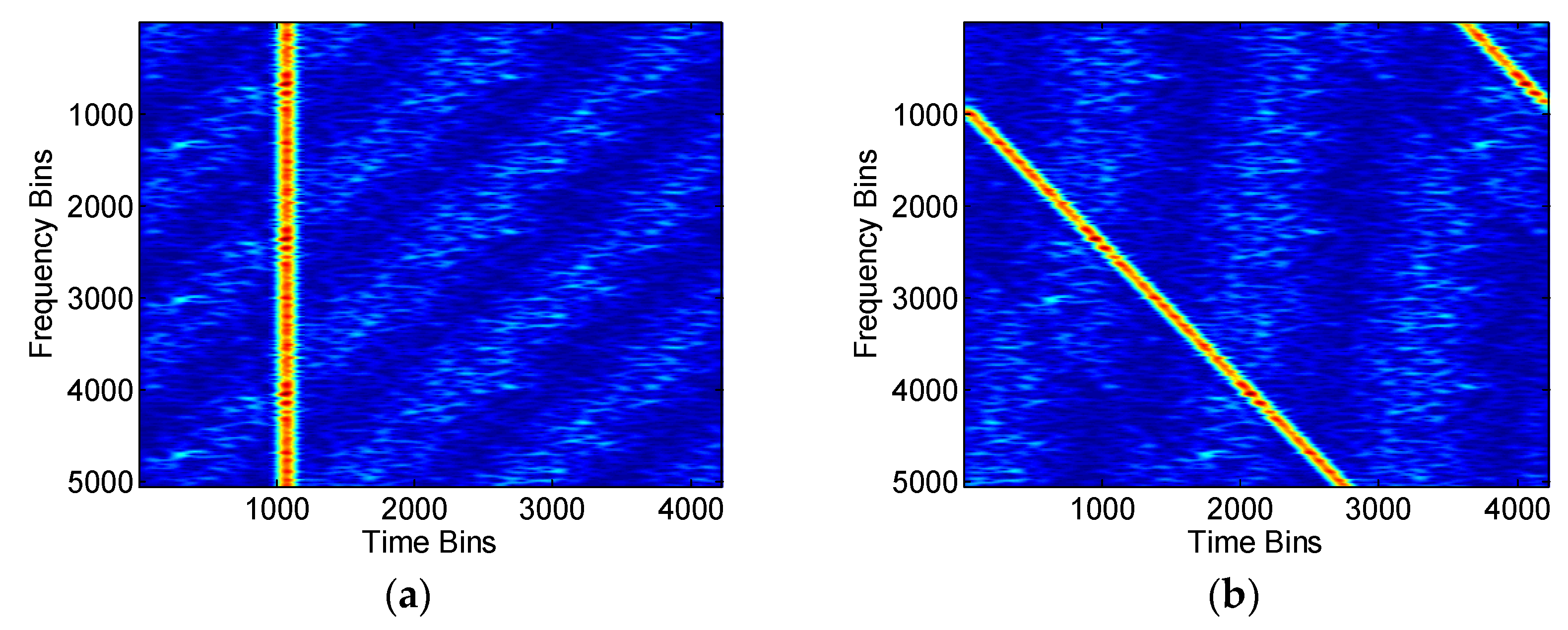
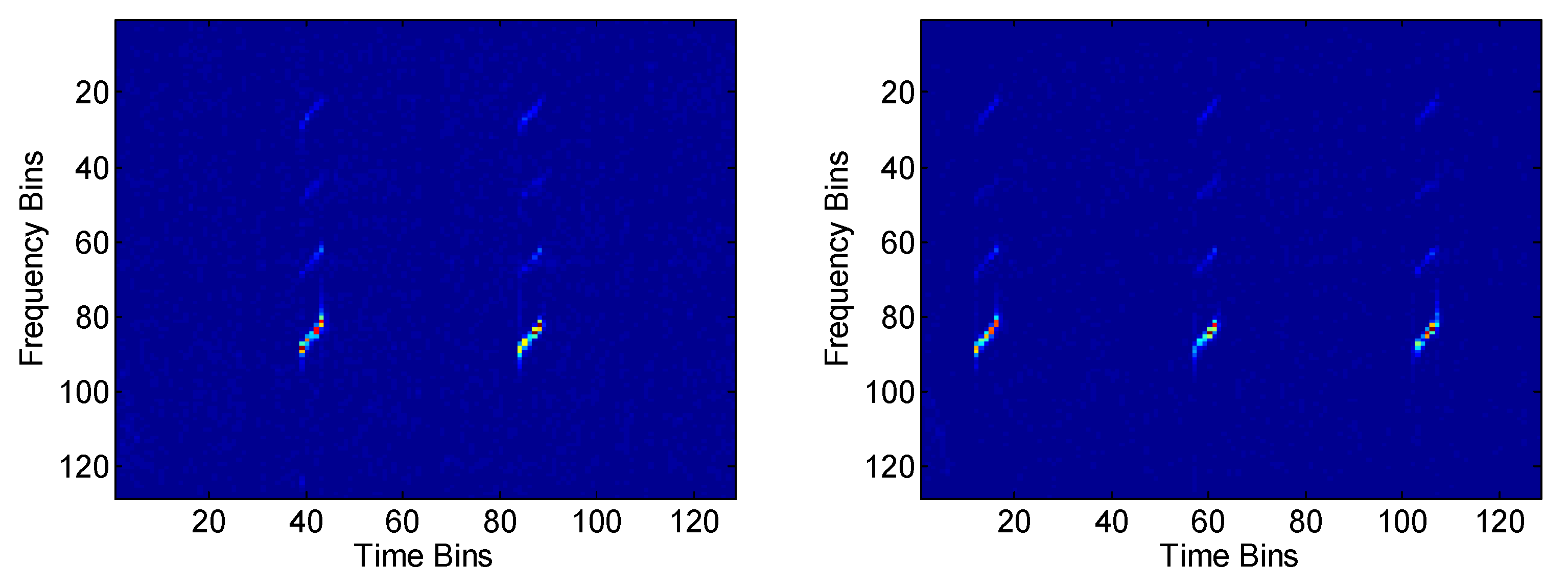
Figure 11 shows two measured NBI-contaminated echoes in the time–frequency domain. The echoes were collected by an X-band airborne SAR working in the strip mode. It can be seen that the NBIs were concentrated into a few frequency bins. The NBIs appear as bright stripes superimposed onto the useful target signal. Before applying the mitigation algorithms, it is necessary to identify whether there is interference in each individual pulse. Figure 12 shows the detection probabilities of the SAR pulses via utilizing the IDN. The pulses whose detection probabilities were larger than the threshold (red line) can be identified as the NBI and the threshold was set to 0.5. Figure 13a shows the imaging result without interference mitigation. It can be seen that the NBIs blurred the SAR imaging result, and the magnitude of NBI varied with azimuth time. Because interference was not matched with the echoes, the interference signal did not accumulate by applying matched filtering. Interference also had stronger energy, so it would appear in the original range-azimuth bin, while also being continuous along the time bins. Therefore, interference looks like bright lines in SAR images. Figure 13b–d show the imaging results after applying the range-spectrum notch filtering, the eigensubspace filtering, and the IMN, respectively. These three methods can achieve good focusing quality, where the villages and farms can be seen clearly. In order to further illustrate the effectiveness of IMN for the NBI, the AG, MSD, and GLD were utilized to evaluate the SAR image quality, and the results are shown in Table 5. Because there was no no-return area in the scene, the MNR was not utilized here. It is shown that the IMN outperformed the range-spectrum notch filtering and eigensubspace filtering in terms of all evaluation metrics. The target edge and contrast in the SAR imaging result following IMN was clearer, which demonstrates the performance improvement of the proposed method.
4.3. Results of the Measured WBI-Corrupted Data
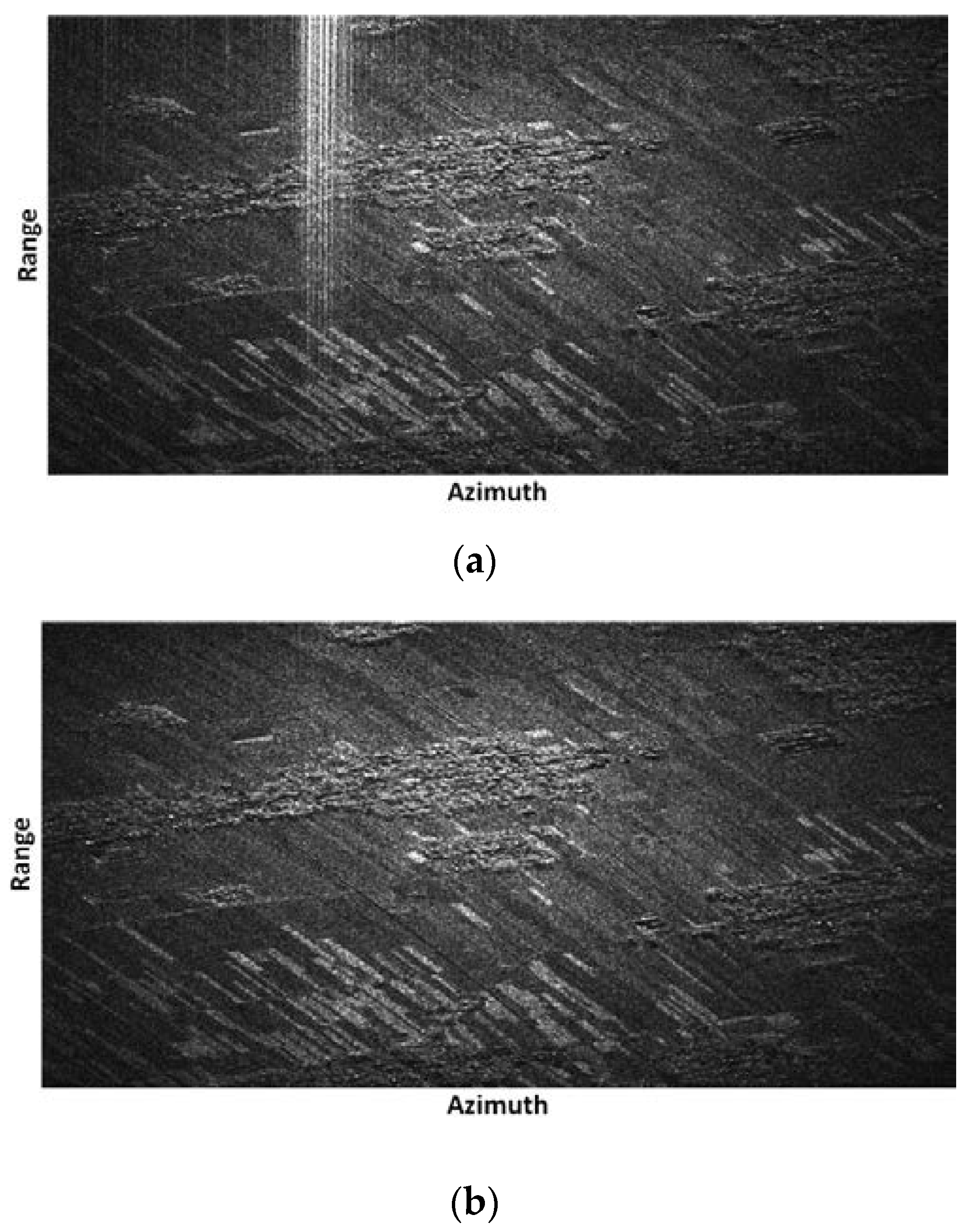
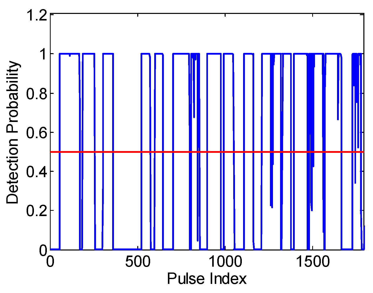
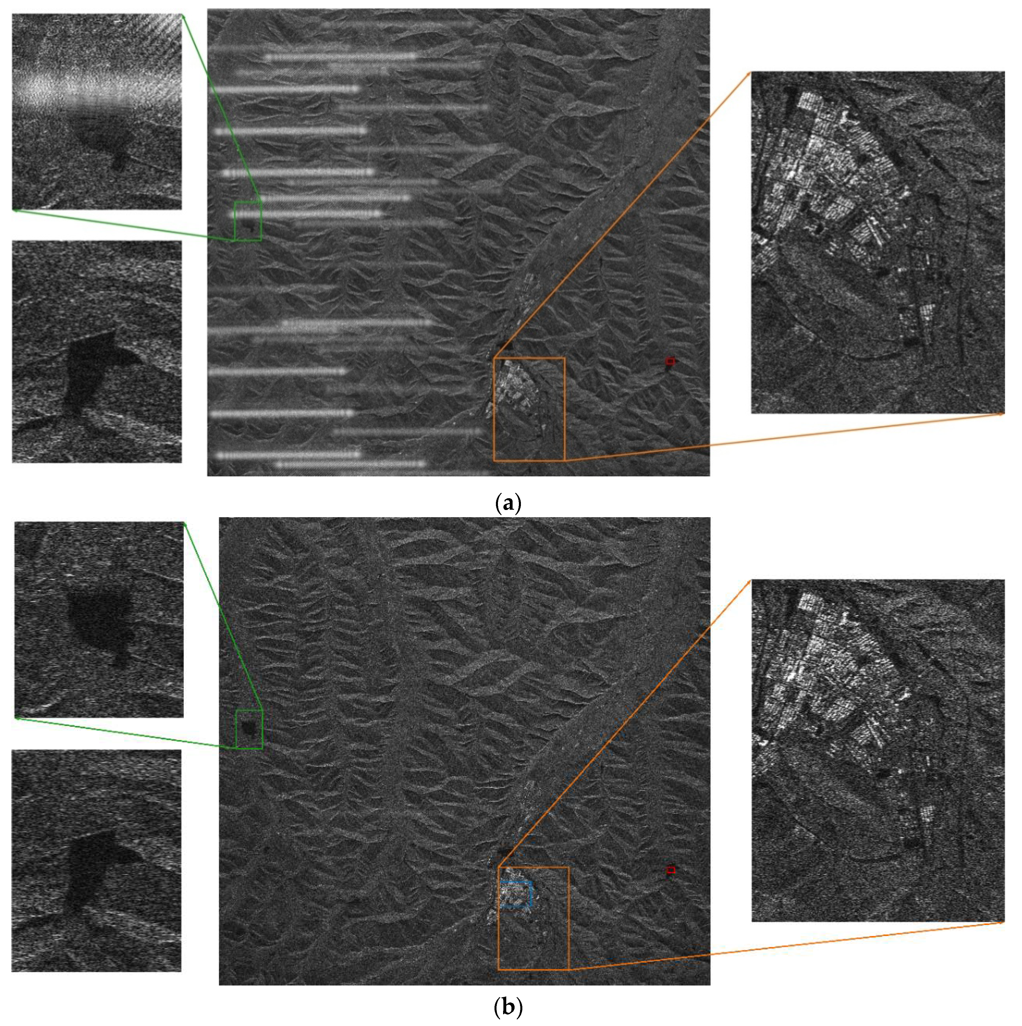
Figure 14 shows an original measured WBI-contaminated echo in the time–frequency domain. The echo was collected by the C-band, dual-pol Sentinel-1A over a mountainous area of western China with the TOPS mode on 25 August 2017. Figure 14a shows the STFT of the WBI-corrupted echo before de-ramping, and the bright vertical line is the WBI signal occupying the entire frequency band. Figure 14b shows the STFT of the WBI-corrupted echoes after de-ramping, and the original WBI signal becomes a Chirp Modulated Wideband Interference (CMWBI). Figure 15 shows the detection probabilities of the SAR pulses by utilizing the IDN, the pulses whose detection probabilities are larger than a threshold (red line) can be identified as WBI signals and the threshold is set to 0.5. Figure 16 shows the imaging result using TOPSAR mode [48] without interference mitigation processing. It can be seen that there are many horizontal bright lines along the range time, which obscure the targets. In order to illustrate the effectiveness of the IMN, the imaging results after different interference mitigation algorithms are shown in Figure 17. Figure 17a shows the zoomed version of the imaging result within the blue box in Figure 16a. The town and roads can be clearly seen from the zoomed result marked by the orange box in Figure 17a. Figure 17b–d show the imaging results after the instantaneous-spectral notch filtering, the eigensubspace filtering, and the IMN, respectively. It can be seen that the WBI signals in the left part have been removed. The town and roads can also be clearly seen with less signal distortion. Moreover, the SAR images marked with green rectangle and red rectangle shown in the left part indicate that these three different methods had similar performances, in which the resulting images were in good focus. To better verify the performance of these three methods, the MNR, AG, MSD, and GLD were utilized for evaluating the SAR image quality, as shown in Table 6. The MNR results for different interference mitigation methods were calculated using the imaging result marked with a blue rectangle and red rectangle, shown in Figure 17. It can be seen that the IMN achieved a better performance than the instantaneous-spectrum notch filtering and the eigensubspace filtering. Meanwhile, the AG, MSD, and GLD of the IMN were larger than the other two methods, which indicates that the targets had more clear edges and better contrast in the SAR imaging result by applying the IMN. Moreover, since the eigensubspace filtering suffers from a higher computational burden because it involves the eigendecomposition, the IMN can decrease the computational burden in the testing stage. The instantaneous-spectral notch filtering, the eigensubspace filtering, and the IMN take about 61.30 s, 1287.02 s, and 61.27s to mitigate WBIs on this measured SAR data, respectively. Figure 16b shows the imaging results after the IMN. Compared with Figure 17, the targets under the interference coverage can be clearly seen in Figure 16b.
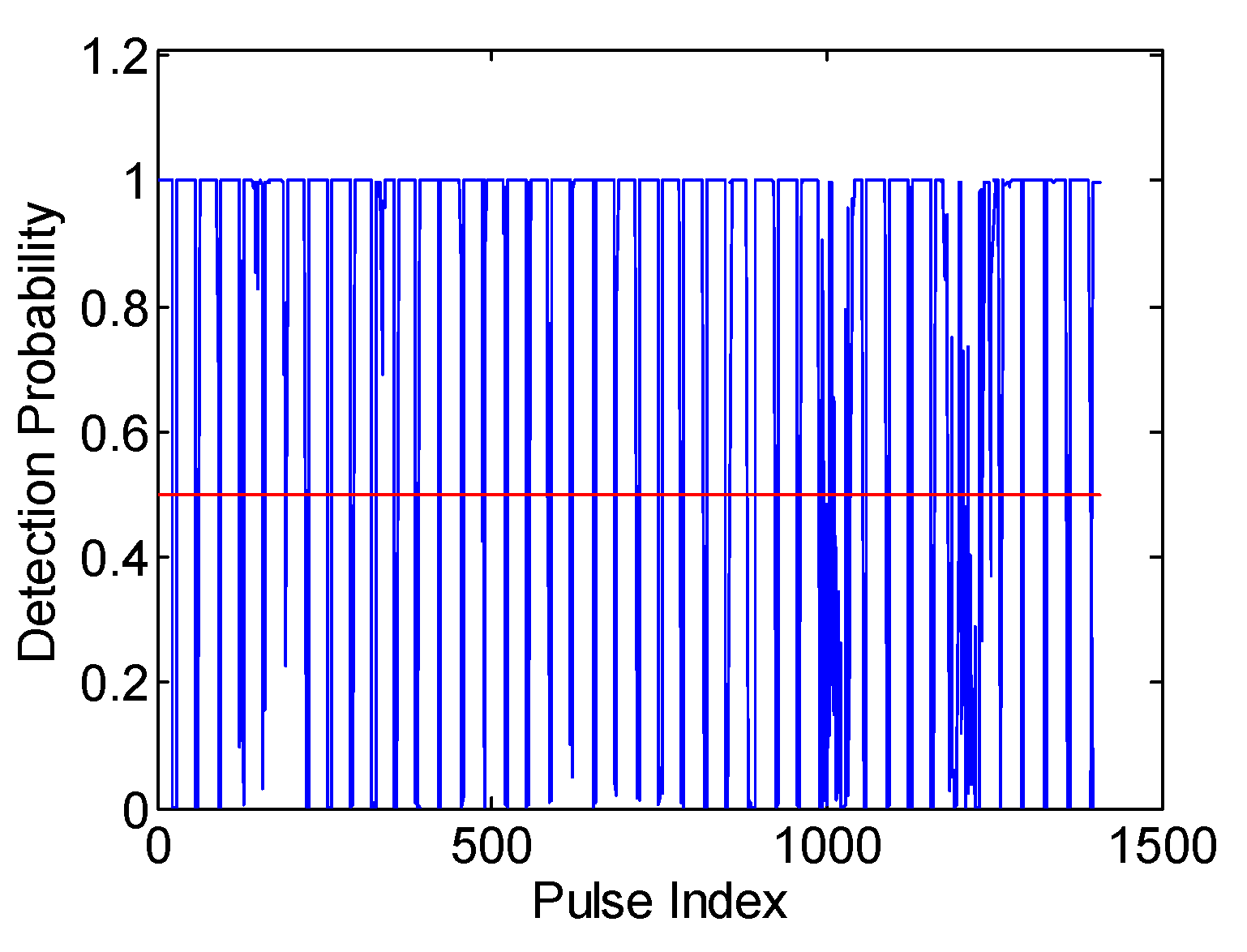
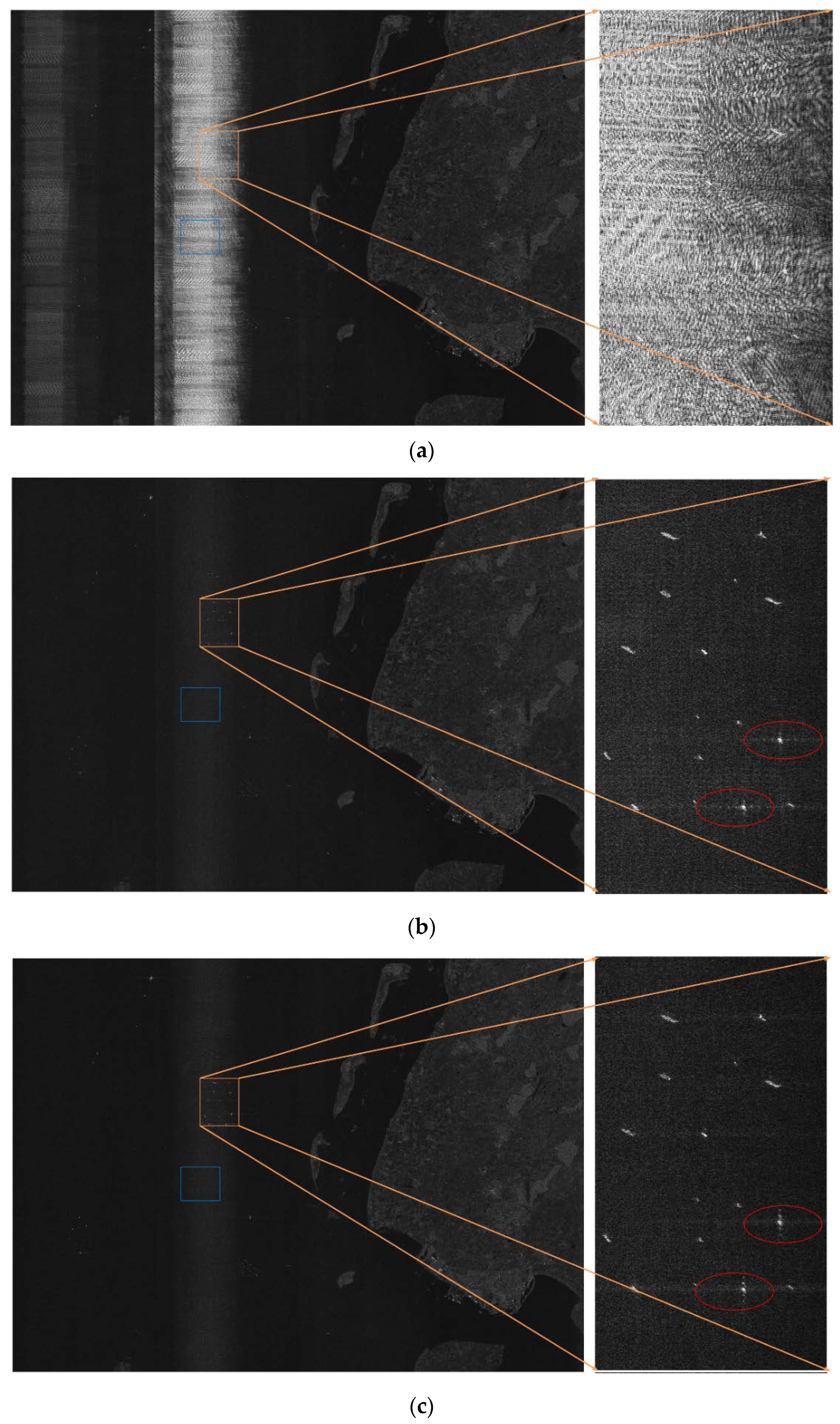
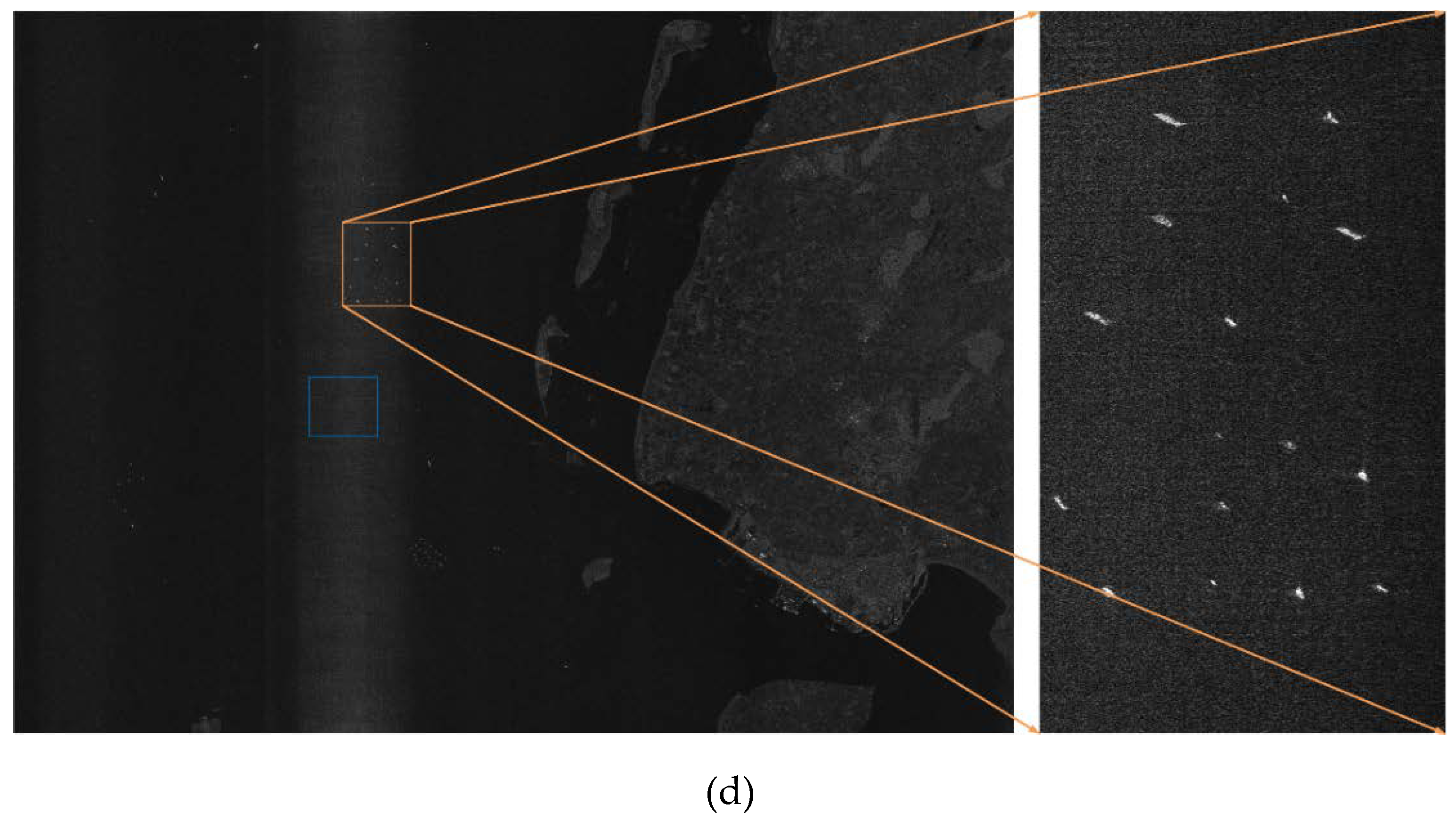
To further evaluate the performance of the IMN, we performed a WBI mitigation experiment for more complicated WBI. This dataset was acquired by European Space Agency (ESA) C-band, dual-pol Sentinel-1B over an area in northeastern Germany on 8 May 2019. Figure 18 shows two measured WBI-contaminated echoes in the time–frequency domain, in which the WBIs are no longer simple lines but have more structure. Figure 19 shows the detection probabilities of the SAR pulses by utilizing the IDN, the pulses whose detection probabilities were larger than the threshold (red line) can be identified as the WBI signals and the threshold was set to 0.5. Figure 20a shows the imaging result using TOPSAR mode [48] without interference mitigation processing. It is shown that interferences obscure the targets completely. Figure 20b–d show the imaging results after the instantaneous-spectral notch filtering, the eigensubspace filtering, and the IMN, respectively. It can be seen that the WBI signals were eliminated by all three mitigation methods, and the ships masked by interference were recovered. Moreover, the zoomed version of the SAR result marked with an orange rectangle is shown in the right part of Figure 20. It can be seen that there are ships marked with a red ellipse that were not well-focused by using the instantaneous-spectral notch filtering and the eigensubspace filtering. The MNR, AG, MSD, and GLD were utilized for evaluating the SAR image quality, as shown in Table 7. The MNR results for different interference mitigation methods were calculated using the imaging results marked with orange and blue rectangles shown in Figure 20. It can be seen that the IMN achieved a better performance than the instantaneous-spectrum notch filtering and the eigensubspace filtering with the AG, MSD, GLD, which indicates that the targets had clearer edges and better contrast in the SAR imaging result when applying the IMN. Meanwhile, the MNR of IMN was smaller than other interference mitigation methods, which indicates that the quality of the SAR image after IMN had a better recovery of system image response. Moreover, the instantaneous-spectral notch filtering, eigensubspace filtering, and the IMN took about 86.41 s, 190.37 s, and 81.64 s to mitigate WBIs on this measured SAR data, respectively. Therefore, the proposed IMN has better interference mitigation performance for WBI.
5. Discussion
In this paper, an interference detection algorithm (IDN) based on DCNN and an interference mitigation algorithm (IMN) based on ResNet were proposed. Compared with previous interference detection algorithms, the IDN utilizes the DCNN to capture the characteristic differences between interference and useful target signal. DCNN has a strong feature extraction ability and is widely applied in the field of image classification. Therefore, it performs well in identifying whether there is interference in echoes. Compared with previous interference mitigation algorithms, the IMN does not need to construct a suitable filter and separate the interference in a specified domain. Instead, it utilizes ResNet to extract useful features of the target signal and reconstruct this signal. ResNet is designed to solve the problem of gradient disappearance within deeper layers of the network and can improve the network’s ability to extract features. Therefore, the IMN can effectively eliminate the effects of interference on an SAR image. One simulated and three measured SAR data were utilized to evaluate the interference detection and mitigation performance of the IMN. The quantitative results indicate a performance gain of the proposed IMN over other methods, as well as its ability to retain the phase of the original signal. Therefore, the IMN can be used in coherent applications like interferometric SAR. The interference mitigation training set only included NBI, CMWBI, and SMWBI. Therefore, the IMN can effectively mitigate the above forms of interference for SAR. However, the mitigation performance may be degraded for some complex forms of interference. In the future, we will include more forms of interference to improve the performance of the proposed framework.
6. Conclusions
In this paper, we proposed an interference detection algorithm (IDN) based on DCNN, which converts the interference detection problem into a two-class classification problem. The network architecture VGG-16 was utilized to train an interference detector and could precisely identify the interference in SAR echoes. We also proposed an interference mitigation algorithm (IMN) based on the deep residual network (ResNet). It extracted the characteristics of the interference and reconstructed the useful target signal in the time–frequency domain, and mitigated the NBI and WBI signals in SAR data effectively. The effectiveness was demonstrated on one simulated dataset and three measured airborne and spaceborne SAR datasets. Moreover, six different metrics, ISR, SDR, MNR, AG, MSD, and GLD, were adopted to assess the performance of the IMN, as well as range-spectrum notch filtering, instantaneous-spectrum notch filtering, and eigensubspace filtering. The IMN can extract features of the useful target signal without the need to design specific feature filters, reducing the complexity of the resulting interference mitigation algorithm.
Author Contributions
For research articles with several authors, a short paragraph specifying their individual contributions must be provided. W. F. conceived and designed the experiment and analyzed the data, W. F., S.Y., P. R. and T. T. performed the experiments, W. F. wrote the paper, F.Z. and M. T. gave lots of advices, M. T. revised the grammar and technical error of the paper and gave lots of advices, X. B improves the English writing skill.
Funding
This paper was funded in part by the China Postdoctoral Science Foundation, grant numbers 2017M613076 and 2016M602775; in part by the National Natural Science Foundation of China, grant numbers 61801347, 61801344, 61522114, 61471284, 61571349, 61631019, 61871459, and 61801390; in part by the NSAF, grant number U1430123; by the Fundamental Research Funds for the Central Universities, grant numbers XJS17070, NSIY031403, and 3102017jg02014; and by the Natural Science Basic Research Plan in Shaanxi Province of China, grant number 2018JM6051; in part by the Aeronautical Science Foundation of China, grant number 20181081003; in part by the Postdoctoral Science Research Projects of Shaanxi Province; and by the Science, Technology and Innovation Commission of Shenzhen Municipality, grant number JCYJ20170306154716846.
Acknowledgments
The authors would like to thank all the anonymous reviewers and editors for their useful comments and suggestions that greatly improved this paper. Meanwhile, the authors are grateful for European Space Agency for providing the sentinel-1A and sentinel-1B data for free downloading.
Conflicts of Interest
The authors declare no conflict of interest.
References
- Moreira, A.; Prats-Iraola, P.; Younis, M.; Krieger, G.; Hajnsek, I.; Papathanassiou, K.P. A tutorial on synthetic aperture radar. IEEE Geosci. Remote Sens. Mag. 2013, 1, 6–43. [Google Scholar] [CrossRef] [Green Version]
- Reigber, A.; Scheiber, R.; Jager, M.; Pau, P.; Hajnsek, I.; Jagdhuber, T. Very-high-resolution airborne synthetic aperture radar imaging: signal processing and applications. Proc. IEEE 2013, 101, 759–783. [Google Scholar] [CrossRef]
- Dudczyk, J.; Kawalec, A.; Cyrek, J. Applying the distance and similarity functions to radar signals identification. In Proceedings of the 2008 International Radar Symposium, Wroclaw, Poland, 21–23 May 2008. [Google Scholar]
- Dudczyk, J.; Kawalec, A. Optimizing the minimum cost flow algorithm for the phase unwrapping process in SAR radar. Bull. Pol. Acad. Sci. Tech. Sci. 2014, 62, 511–516. [Google Scholar] [CrossRef] [Green Version]
- Matuszewski, J. Radar signal identification using a neural network and pattern recognition methods. In Proceedings of the 2018 14th International Conference on Advanced Trends in Radioelecrtronics, Telecommunications and Computer Engineering (TCSET), Lviv-Slavske, Ukraine, 20–24 February 2018; pp. 79–83. [Google Scholar]
- Kim, A.; Dogan, S.; Fisher, J., III; Moses, R.; Willsky, A. Attributing scatterer anisotropy for model based ATR. In Proceedings of the International Society for Optical Engineering, Orlando, FL, USA, 24–28 April 2000; pp. 176–188. [Google Scholar]
- Sadjadi, A. New experiments in inverse synthetic aperture radar image exploitation for maritime surveillance, In Proceedings of the International Society for Optical Engineering, Baltimore, MD, USA, 5–6 May 2014.
- Meyer, F.; Nicoll, J.; Doulgeris, A. Correction and characterization of radio frequency interference signatures in l-band syntheticaperture radar data. IEEE Trans. Geosci. Remote Sens. 2013, 51, 4961–4972. [Google Scholar] [CrossRef]
- Su, J.; Tao, H.; Tao, M.; Wang, L.; Xie, J. Narrow-band interference suppression via rpca-based signal separation in time–frequency domain. IEEE J. Sel. Top. Appl. Earth Obs. Remote Sens. 2017, 10, 5016–5025. [Google Scholar] [CrossRef]
- Zhou, F.; Xing, M.; Bai, X.; Sun, G.; Bao, Z. Narrow-band interference suppression for sar based on complex empirical mode decomposition. IEEE Trans. Geosci. Remote Sens. 2012, 50, 3202–3218. [Google Scholar]
- Zhou, F.; Tao, M. Research on methods for narrow-band interference suppression in synthetic aperture radar data. IEEE J. Sel. Top. Appl. Earth Obs. 2015, 8, 3476–3485. [Google Scholar] [CrossRef]
- Tao, M.; Zhou, F.; Zhang, Z. Wideband interference mitigation in high-resolution airborne synthetic aperture radar data. IEEE Trans. Geosci. Remote Sens. 2016, 54, 74–87. [Google Scholar] [CrossRef]
- Su, J.; Tao, H.; Tao, M.; Xie, J.; Wang, Y.; Wang, L. Time-Varying SAR Interference Suppression Based on Delay-Doppler Iterative Decomposition Algorithm. Remote Sens. 2018, 10, 1491. [Google Scholar] [CrossRef]
- Yu, J.; Li, J.; Sun, B.; Chen, J.; Li, C. Multiclass Radio Frequency Interference Detection and Suppression for SAR Based on the Single Shot MultiBox Detector. Sensors 2018, 18, 4034. [Google Scholar] [CrossRef]
- Nguyen, L.; Soumekh, M. Suppression of radio frequency interference (RFI) for synchronous impulse reconstruction ultra-wideband radar. Proc. SPIE 2005, 5808, 178–184. [Google Scholar]
- Yi, J.; Wan, X.; Cheng, F.; Gong, Z. Computationally efficient RF interference suppression method with closed-form maximum likelihoodestimator for HF surface wave over-the-horizon radars. IEEE Trans. Geosci. Remote Sens. 2013, 51, 2361–2372. [Google Scholar] [CrossRef]
- Ojowu, O.; Li, J. RFI suppression for synchronous impulse reconstruction UWB radar using RELAX. Int. J. Remote Sens. Appl. 2013, 3, 33–46. [Google Scholar]
- Guo, Y.; Zhou, F.; Tao, M.; Sheng, M. A new method for sar radio frequency interference mitigation based on maximum a posterior estimation. In Proceedings of the 2017 32nd General Assembly and Scientific Symposium of the International Union of Radio Science, Montreal, QC, Canada, 19–26 August 2017; pp. 1–4. [Google Scholar]
- Reigber, A.; Ferro-Famil, L. Interference suppression in synthesized sar images. IEEE Geosci. Remote Sens. Lett. 2005, 2, 45–49. [Google Scholar] [CrossRef]
- Smith, L.; Hill, R.; Hayward, S.; Yates, G.; Blake, A. Filtering approaches for interference suppression in low-frequency sar. IEE Radar Sonar Navig. 2006, 153, 338–344. [Google Scholar] [CrossRef]
- Zhou, F.; Wu, R.; Xing, M.; Bao, Z. Eigensubpace-based filtering with application in narrow-band interference suppression for sar. IEEE Geosci. Remote Sens. Lett. 2007, 4, 75–79. [Google Scholar] [CrossRef]
- Wang, X.; Yu, W.; Qi, X.; Liu, Y. RFI suppression in SAR based on approximate spectral decomposition algorithm. Electron. Lett. 2012, 48, 594–596. [Google Scholar] [CrossRef]
- Feng, J.; Zheng, H.; Deng, Y.; Gao, D. Application of subband spectral cancellation for sar narrow-band interference suppression. IEEE Geosci. Remote Sens. Lett. 2012, 9, 190–193. [Google Scholar] [CrossRef]
- Spencer, M.; Chen, C.; Ghaemi, H.; Chan, S.; Belz, J. RFI characterization and mitigation for the smap radar. IEEE Trans. Geosci. Remote Sens. 2013, 51, 4973–4982. [Google Scholar] [CrossRef]
- Huang, Y.; Liao, G.; Li, J.; Xu, J. Narrowband RFI suppression for sar system via fast implementation of joint sparsity and low-rank property. IEEE Trans. Geosci. Remote Sens. 2018, 56, 2748–2761. [Google Scholar] [CrossRef]
- Huang, Y.; Liao, G.; Xu, J.; Li, J. Narrowband RFI suppression for sar system via efficient parameter-free decomposition algorithm. IEEE Trans. Geosci. Remote Sens. 2018, 56, 3311–3321. [Google Scholar] [CrossRef]
- Krizhevsky, A.; Sutskever, I.; Hinton, G. ImageNet classification with deep convolutional neural networks. In Proceeding of the 2012 Advances in Neural Information Processing Systems (NIPS), Lake Tahoe, NV, USA, 3–6 December 2012; pp. 1097–1105. [Google Scholar]
- Simonyan, K.; Zisserman, A. Very deep convolutional networks for large-scale image recognition. In Proceedings of the 2015 International Conference Learning Representations (ICLR), New York, NY, USA, 7–9 May 2015; pp. 1–14. [Google Scholar]
- He, K.; Zhang, X.; Ren, S.; Sun, J. Deep residual learning for image recognition. In Proceedings of the 2016 IEEE Conference on Computer Vision and Pattern Recognition (CVPR), Las Vegas, NV, USA, 26 June–1 July 2016; pp. 770–778. [Google Scholar]
- Girshick, R.; Donahue, J.; Darrell, T.; Malik, J. Rich feature hierarchies for accurate object detection and semantic segmentation. In Proceedings of the 2014 IEEE Conference on Computer Vision and Pattern Recognition (CVPR), Columbus, OH, USA, 23–28 June 2014; pp. 580–587. [Google Scholar]
- Ren, S.; He, K.; Girshick, R.; Sun, J. Faster r-cnn: towards real-time object detection with region proposal networks. IEEE Trans. Pattern Anal. Mach. Intell. 2017, 39, 1137–1149. [Google Scholar] [CrossRef] [PubMed]
- Redmon, J.; Divvala, S.; Girshick, S.; Farhadi, A. You only look once: unified, real-time object detection. In Proceedings of the 2016 IEEE Computer Society Conference on Computer Vision and Pattern Recognition (CVPR), Las Vegas, NV, USA, 26 June–1 July 2016; pp. 779–788. [Google Scholar]
- Shelhamer, E.; Long, J.; Darrell, T. Fully convolutional networks for semantic segmentation. IEEE Trans. Pattern Anal. Mach. Intell. 2017, 39, 640–651. [Google Scholar] [CrossRef] [PubMed]
- Dronner, J.; Korfhage, N.; Egli, S.; Muhling, M.; Thies, B.; Bendix, J.; Freisleben, B.; Seeger, B. Fast cloud segmentation using convolutional neural networks. Remote Sens. 2018, 10, 1782. [Google Scholar] [CrossRef]
- Noh, H.; Hong, S.; Han, B. Learning deconvolution network for semantic segmentation. In Proceedings of the 2015 IEEE International Conference on Computer Vision (ICCV), Santiago, Chile, 11–18 December 2015; pp. 1520–1528. [Google Scholar]
- Wang, P.; Zhang, H.; Patel, V. Generative adversarial network-based restoration of speckled SAR images. In Proceedings of the 2017 IEEE 7th International Workshop on Computational Advances in Multi-Sensor Adaptive Processing (CAMSAP), Curacao, Netherlan, 10–13 December 2017; pp. 1–5. [Google Scholar]
- Michelsanti, D.; Tan, Z. Conditional generative adversarial networks for speech enhancement and noise-robust speaker verification. In Proceedings of the Annual Conference of the International Speech Communication Association, Stockholm, Sweden, 20–24 August 2017; pp. 2008–2012. [Google Scholar]
- Ledig, C.; Theis, L.; Huszar, F.; Caballero, J.; Cunningham, A.; Acosta, A.; Aitken, A.; Tejani, A.; Totz, J.; Wang, Z.; et al. Photo-realistic single image super-resolution using a generative adversarial network. In Proceedings of the 2017 IEEE Conference on Computer Vision and Pattern Recognition (CVPR), Honolulu, Hawaii, HI, USA, 21–26 July 2017; pp. 105–114. [Google Scholar]
- Zhao, W.; Wang, D.; Lu, H. Multi-focus image fusion with a natural enhancement via joint multi-level deeply supervised convolutional neural network. IEEE Trans. Circuits Syst. Video Technol. 2018, 29, 1102–1115. [Google Scholar] [CrossRef]
- Goodfellow, I.; Pouget-Abadie, J.; Mirza, M.; Xu, B.; Warde-Farley, D.; Ozair, S.; Courville, A.; Bengio, Y. Generative adversarial networks. In Proceeding of the 2014 Advances in Neural Information Processing Systems (NIPS), Montreal, AB, Canada, 8–11 December 2014; pp. 2672–2680. [Google Scholar]
- Arjovsky, M.; Chintala, S.; Bottou, L. Wasserstein generative adversarial networks. In Proceedings of the 34th International Conference on Machine Learning (ICML), Sydney, Australia, 6–11 August 2017; pp. 298–321. [Google Scholar]
- Isola, P.; Zhu, J.; Zhou, T.; Efros, A. Image-to-image translation with conditional adversarial networks. In Proceedings of the 2017 IEEE Conference on Computer Vision and Pattern Recognition (CVPR), Honolulu, Hawaii, HI, USA, 21–26 July 2017; pp. 5967–5976. [Google Scholar]
- Wang, C.; Xu, C.; Wang, C.; Tao, D. Perceptual adversarial networks for image-to-image transformation. IEEE Trans. Image Process. 2018, 27, 4066–4079. [Google Scholar] [CrossRef] [PubMed]
- Abadi, M.; Barham, P.; Chen, J.; Chen, Z.; Davis, A.; Dean, J.; Devin, M.; Ghemawat, S.; Irving, G.; Isard, M.; et al. Tensorflow: A system for large-scale machine learning. In Proceedings of the 12th {USENIX} Symposium on Operating Systems Design and Implementation ({OSDI} 16), Savannah, GA, USA; 2016; pp. 265–283. [Google Scholar]
- Kingma, D.; Adam, B. A method for stochastic optimization. In Proceedings of the 2014 International Conference on Learning Representations (ICLR), Banff, AB, Canada, 14–16 April 2014; pp. 1–15. [Google Scholar]
- Cui, G.; Feng, H.; Xu, Z.; Li, Q.; Chen, Y. Detail preserved fusion of visible and infrared images using regional saliency extraction and multi-scale image decomposition. Opt. Commun. 2015, 341, 199–209. [Google Scholar] [CrossRef]
- Li, Z.; Liu, C. Gray level difference-based transition region extraction and thresholding. Comput. Electr. Eng. 2009, 35, 696–704. [Google Scholar] [CrossRef]
- Zan, F.; Guarnieri, A. Topsar: terrain observation by progressive scans. IEEE Trans. Geosci. Remote Sens. 2006, 44, 2352–2360. [Google Scholar] [CrossRef]
Figure 1.
Synthetic Aperture Radar (SAR) echoes corrupted with (a) and (b) narrow-band interference (NBI) in range-frequency azimuth-time domain and wide-band interference (WBI) in azimuth-frequency range-time domain.
Figure 1.
Synthetic Aperture Radar (SAR) echoes corrupted with (a) and (b) narrow-band interference (NBI) in range-frequency azimuth-time domain and wide-band interference (WBI) in azimuth-frequency range-time domain.

Figure 2.
An example of the (a) NBI-corrupted echo in the range-time domain, (b) NBI-corrupted echo in the range-frequency domain, (c) NBI-corrupted echo in the time–frequency domain, (d) WBI-corrupted echo in the azimuth-time domain, (e) WBI-corrupted echo in the azimuth-frequency domain, and (f) WBI-corrupted echo in the time–frequency domain.

Figure 3.
The interference detection network (IDN) framework.

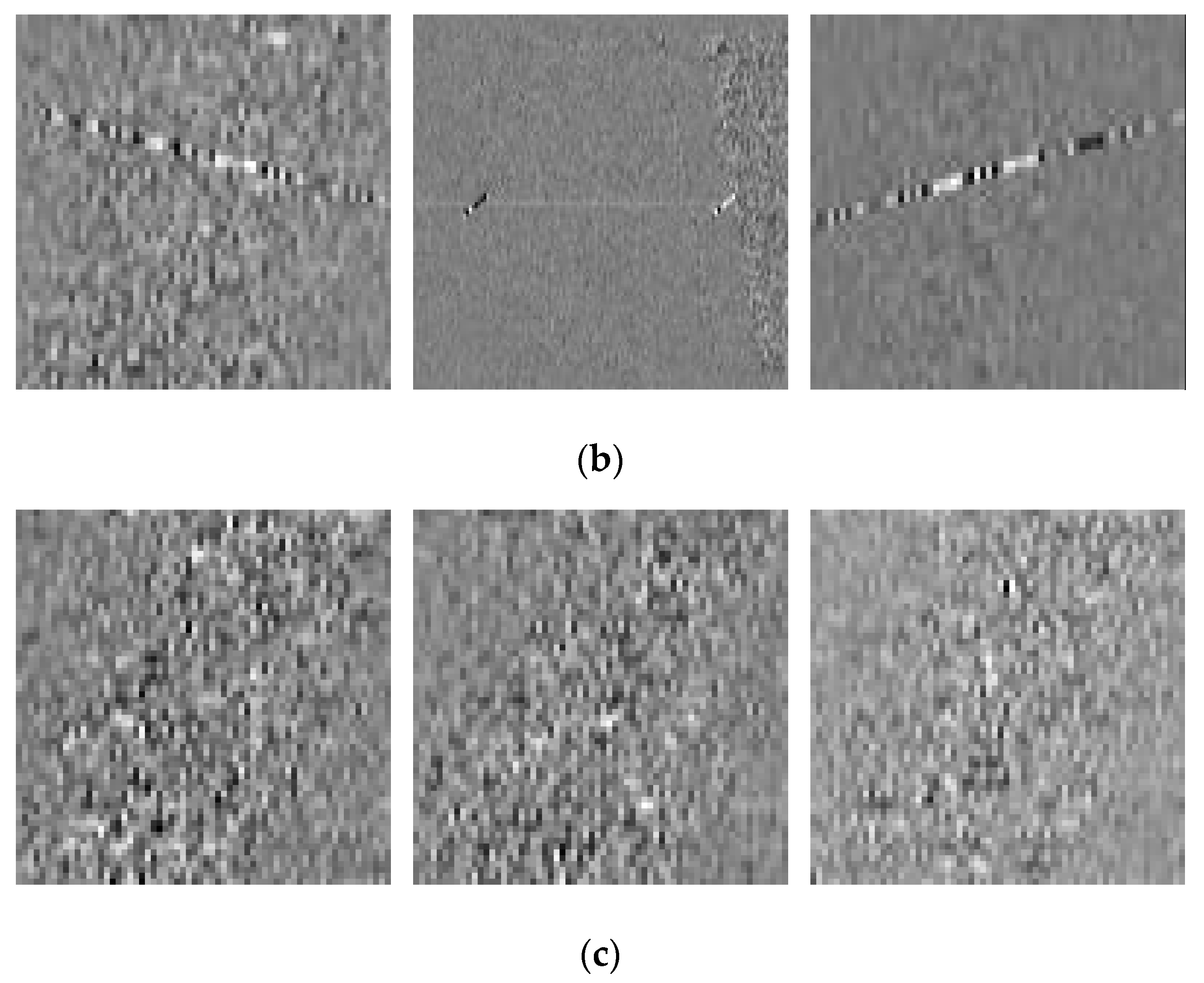
Figure 4.
Samples of echoes in time–frequency representation used for training the IDN. (a) Shows the NBI-corrupted echoes, (b) shows the WBI-corrupted echoes, and (c) shows the echoes without interference.
Figure 4.
Samples of echoes in time–frequency representation used for training the IDN. (a) Shows the NBI-corrupted echoes, (b) shows the WBI-corrupted echoes, and (c) shows the echoes without interference.


Figure 5.
The interference mitigation network (IMN) framework.

Figure 6.
Workflow of the interference detection and mitigation based on a deep convolutional neural network (DCNN).
Figure 6.
Workflow of the interference detection and mitigation based on a deep convolutional neural network (DCNN).

Figure 7.
Simulated SAR echoes in the time–frequency domain for training and testing the IMN. (a) the original SAR echoes without interference, and (b) the interference-corrupted echoes.
Figure 7.
Simulated SAR echoes in the time–frequency domain for training and testing the IMN. (a) the original SAR echoes without interference, and (b) the interference-corrupted echoes.

Figure 8.
The convergence curve of training accuracy with training iterations.

Figure 9.
Representation in the time–frequency domain. (a) Short-time Fourier transform (STFT) of the NBI-free pulse. (b) STFT of the simulated NBI-corrupted pulse. (c) STFT after the range spectrum notch filtering. (d) STFT after the eigensubspace filtering. (e) STFT after the IMN.
Figure 9.
Representation in the time–frequency domain. (a) Short-time Fourier transform (STFT) of the NBI-free pulse. (b) STFT of the simulated NBI-corrupted pulse. (c) STFT after the range spectrum notch filtering. (d) STFT after the eigensubspace filtering. (e) STFT after the IMN.

Figure 10.
Representation in the time–frequency domain. (a) STFT of the WBI-free pulse. (b) STFT of the simulated WBI-corrupted pulse. (c) STFT after the instantaneous-spectrum notch filtering. (d) STFT after the eigensubspace filtering. (e) STFT after the IMN.
Figure 10.
Representation in the time–frequency domain. (a) STFT of the WBI-free pulse. (b) STFT of the simulated WBI-corrupted pulse. (c) STFT after the instantaneous-spectrum notch filtering. (d) STFT after the eigensubspace filtering. (e) STFT after the IMN.

Figure 11.
The representation of the (a) 500th and (b) 1000th measured NBI-contaminated echoes in the time–frequency domain.
Figure 11.
The representation of the (a) 500th and (b) 1000th measured NBI-contaminated echoes in the time–frequency domain.

Figure 12.
The detection probability of radar pulse before NBI mitigation, where the red line represents the threshold.
Figure 12.
The detection probability of radar pulse before NBI mitigation, where the red line represents the threshold.

Figure 13.
Mitigation results. (a) the SAR image without interference mitigation, (b) the SAR image after applying the range-spectrum notch filtering, (c) the SAR image after applying the eigensubspace filtering, and (d) the SAR image after applying the IMN.
Figure 13.
Mitigation results. (a) the SAR image without interference mitigation, (b) the SAR image after applying the range-spectrum notch filtering, (c) the SAR image after applying the eigensubspace filtering, and (d) the SAR image after applying the IMN.


Figure 14.
The representation of the measured WBI-contaminated echoes in the time–frequency domain. (a) The STFT of the WBI-contaminated echo before de-ramping, and (b) the STFT of the WBI-contaminated echo after de-ramping.
Figure 14.
The representation of the measured WBI-contaminated echoes in the time–frequency domain. (a) The STFT of the WBI-contaminated echo before de-ramping, and (b) the STFT of the WBI-contaminated echo after de-ramping.

Figure 15.
The detection probability of radar pulse before WBI mitigation, where the red line represents the threshold.
Figure 15.
The detection probability of radar pulse before WBI mitigation, where the red line represents the threshold.

Figure 16.
The SAR imaging results (a) without interference mitigation and (b) after IMN.

Figure 17.
Mitigation results. (a) The SAR image without interference mitigation, (b) the SAR image after applying the instantaneous-spectrum notch filtering, (c) the SAR image after applying the eigensubspace filtering, and (d) the SAR image after applying the IMN.
Figure 17.
Mitigation results. (a) The SAR image without interference mitigation, (b) the SAR image after applying the instantaneous-spectrum notch filtering, (c) the SAR image after applying the eigensubspace filtering, and (d) the SAR image after applying the IMN.


Figure 18.
The representation of two measured WBI-contaminated echoes in the time–frequency domain.

Figure 19.
The detection probability of radar pulse before WBI mitigation, where the red line represents the threshold.
Figure 19.
The detection probability of radar pulse before WBI mitigation, where the red line represents the threshold.

Figure 20.
Mitigation results. (a) The SAR image without interference mitigation, (b) the SAR image after applying the instantaneous-spectrum notch filtering, (c) the SAR image after applying the eigensubspace filtering, and (d) the SAR image after applying the IMN.
Figure 20.
Mitigation results. (a) The SAR image without interference mitigation, (b) the SAR image after applying the instantaneous-spectrum notch filtering, (c) the SAR image after applying the eigensubspace filtering, and (d) the SAR image after applying the IMN.


Table 1.
IDN Architecture.
| Input: Images in the Temporal–Frequency Domain | |
|---|---|
| Layer 1 | Conv. (3,3,64), stride = 1; ReLU layer; |
| Layer 2 | Conv. (3,3,64), stride = 1; ReLU layer; |
| Layer 3 | MP. (2,2), stride = 2; |
| Layer 4 | Conv. (3,3,128), stride = 1; ReLU layer; |
| Layer 5 | Conv. (3,3,128), stride = 1; ReLU layer; |
| Layer 6 | MP. (2,2), stride = 2; |
| Layer 7 | Conv. (3,3,256), stride = 1; ReLU layer; |
| Layer 8 | Conv. (3,3,256), stride = 1; ReLU layer; |
| Layer 9 | Conv. (3,3,256), stride = 1; ReLU layer; |
| Layer 10 | MP. (2,2), stride = 2; |
| Layer 11 | Conv. (3,3,512), stride = 1; ReLU layer; |
| Layer 12 | Conv. (3,3,512), stride = 1; ReLU layer; |
| Layer 13 | Conv. (3,3,512), stride = 1; ReLU layer; |
| Layer 14 | MP. (2,2), stride = 2; |
| Layer 15 | Conv. (3,3,512), stride = 1; ReLU layer; |
| Layer 16 | Conv. (3,3,512), stride = 1; ReLU layer; |
| Layer 17 | Conv. (3,3,512), stride = 1; ReLU layer; |
| Layer 18 | MP. (2,2), stride = 2; |
| Layer 19 | Fc. (1,1,4096); |
| Layer 20 | Fc. (1,1,4096); |
| Layer 21 | Fc. (1,1,2); |
| Layer 22 | Softmax layer. |
Table 2.
The IMN Architecture.
| Interference Mitigation Network | |
|---|---|
| Input: Images in the Temporal–Frequency Domain | |
| Layer 1 | Conv. (3,3,64), stride = 1; ReLU layer; |
| Block 1 | Conv. (3,3,64), stride = 1; BN; ReLU layer; Conv. (3,3,64), stride = 1; BN; Es. (Layer 1); |
| Block 2 | Conv. (3,3,64), stride = 1; BN; ReLU layer; Conv. (3,3,64), stride = 1; BN; Es. (Block 1); |
| …… | |
| Block 16 | Conv. (3,3,64), stride = 1; BN; ReLU layer; Conv. (3,3,64), stride = 1; BN; Es. (Block 15); |
| Layer 18 | Conv. (3,3,64), stride = 1; BN; Es. (Layer 1); |
| Layer 19 | Conv. (3,3,64), stride=1. |
Table 3.
Comparison for the simulated NBI-contaminated echo.
| Range-Spectrum Notch Filtering | Eigensubspace Filtering | IMN | Improvement (%) | |
|---|---|---|---|---|
| ISR(dB) | 5.08 | 5.09 | 5.32 | 4.72/4.52 |
| SDR(dB) | −11.66 | −11.75 | −12.32 | 5.66/4.81 |
Table 4.
Comparison for the WBI-contaminated echo.
| Instantaneous-Spectrum Notch Filtering | Eigensubspace Filtering | IMN | Improvement (%) | |
|---|---|---|---|---|
| ISR(dB) | 5.47 | 5.49 | 5.49 | 0.37/0.00 |
| SDR(dB) | –9.62 | –10.22 | –12.77 | 32.74/24.95 |
Table 5.
The SAR image quality evaluation for the measured NBI-contaminated data.
| Range Spectrum Notch Filtering | Eigensubspace Filtering | IMN | Improvement (%) | |
|---|---|---|---|---|
| AG | 4.926 | 4.974 | 5.288 | 7.35/6.31 |
| MSD | 0.049 | 0.050 | 0.052 | 6.12/4.00 |
| GLD | 41.561 | 41.941 | 44.524 | 7.13/6.16 |
Table 6.
SAR image quality evaluation for the measured WBI-contaminated data.
| Instantaneous Spectrum Notch Filtering | Eigensubspace Filtering | IMN | Improvement (%) | |
|---|---|---|---|---|
| MNR (dB) | −15.03 | −15.43 | −15.72 | 4.59/1.88 |
| AG | 6.25 | 6.41 | 6.69 | 7.04/4.37 |
| MSD | 0.052 | 0.053 | 0.055 | 5.77/3.77 |
| GLD | 50.407 | 51.747 | 53.875 | 6.88/4.11 |
Table 7.
SAR image quality evaluation for the measured WBI-contaminated data.
| Instantaneous Spectrum Notch Filtering | Eigensubspace Filtering | IMN | Improvement (%) | |
|---|---|---|---|---|
| MNR (dB) | –0.43 | –0.60 | –0.64 | 48.84/6.67 |
| AG | 3.55 | 3.21 | 3.83 | 7.89/19.31 |
| MSD | 0.013 | 0.012 | 0.015 | 15.38/25.00 |
| GLD | 29.16 | 26.20 | 30.85 | 5.80/17.75 |
© 2019 by the authors. Licensee MDPI, Basel, Switzerland. This article is an open access article distributed under the terms and conditions of the Creative Commons Attribution (CC BY) license (http://creativecommons.org/licenses/by/4.0/).
Share and Cite
MDPI and ACS Style
Fan, W.; Zhou, F.; Tao, M.; Bai, X.; Rong, P.; Yang, S.; Tian, T. Interference Mitigation for Synthetic Aperture Radar Based on Deep Residual Network. Remote Sens. 2019, 11, 1654. https://0-doi-org.brum.beds.ac.uk/10.3390/rs11141654
AMA Style
Fan W, Zhou F, Tao M, Bai X, Rong P, Yang S, Tian T. Interference Mitigation for Synthetic Aperture Radar Based on Deep Residual Network. Remote Sensing. 2019; 11(14):1654. https://0-doi-org.brum.beds.ac.uk/10.3390/rs11141654
Chicago/Turabian StyleFan, Weiwei, Feng Zhou, Mingliang Tao, Xueru Bai, Pengshuai Rong, Shuang Yang, and Tian Tian. 2019. "Interference Mitigation for Synthetic Aperture Radar Based on Deep Residual Network" Remote Sensing 11, no. 14: 1654. https://0-doi-org.brum.beds.ac.uk/10.3390/rs11141654
Note that from the first issue of 2016, this journal uses article numbers instead of page numbers. See further details here.