Article

SmokeNet: Satellite Smoke Scene Detection Using Convolutional Neural Network with Spatial and Channel-Wise Attention

1
State Key Laboratory of Fire Science, University of Science and Technology of China, Jinzhai 96, Hefei 230026, China
2
Department of Civil and Architectural Engineering, City University of Hong Kong, Tat Chee Avenue, Kowloon, Hong Kong, China
3
Department of Electrical and Computer Engineering, The University of North Carolina at Charlotte, Charlotte, NC 28223, USA
*
Author to whom correspondence should be addressed.
Remote Sens. 2019, 11(14), 1702; https://0-doi-org.brum.beds.ac.uk/10.3390/rs11141702
Submission received: 31 May 2019 / Revised: 15 July 2019 / Accepted: 16 July 2019 / Published: 18 July 2019

Abstract

:
A variety of environmental analysis applications have been advanced by the use of satellite remote sensing. Smoke detection based on satellite imagery is imperative for wildfire detection and monitoring. However, the commonly used smoke detection methods mainly focus on smoke discrimination from a few specific classes, which reduces their applicability in different regions of various classes. To this end, in this paper, we present a new large-scale satellite imagery smoke detection benchmark based on Moderate Resolution Imaging Spectroradiometer (MODIS) data, namely USTC_SmokeRS, consisting of 6225 satellite images from six classes (i.e., cloud, dust, haze, land, seaside, and smoke) and covering various areas/regions over the world. To build a baseline for smoke detection in satellite imagery, we evaluate several state-of-the-art deep learning-based image classification models. Moreover, we propose a new convolution neural network (CNN) model, SmokeNet, which incorporates spatial and channel-wise attention in CNN to enhance feature representation for scene classification. The experimental results of our method using different proportions (16%, 32%, 48%, and 64%) of training images reveal that our model outperforms other approaches with higher accuracy and Kappa coefficient. Specifically, the proposed SmokeNet model trained with 64% training images achieves the best accuracy of 92.75% and Kappa coefficient of 0.9130. The model trained with 16% training images can also improve the classification accuracy and Kappa coefficient by at least 4.99% and 0.06, respectively, over the state-of-the-art models.

Graphical Abstract

1. Introduction

Wildfire is a destructive natural disaster that poses serious threats for human lives, property, and ecosystems [1]. The smoke emitted by biomass burning perturbs the atmospheric radiation balance, air quality, and ecological energy budget [2,3]. However, fire smoke can also be a significant signal of biomass burning, which plays an important role in wildfire detection. Therefore, improved smoke detection is important in the identification of new fires, as well as in the subsequent fire rescue and emergency management [4]. With the rapid development in the past decades, satellite remote sensing brings a great opportunity for this task with the advantages of timeliness, wide observation, and low cost [5]. Nevertheless, the identification of smoke using satellite data is challenging because the fire smoke has varying shapes, colors, scopes, and spectral overlaps [2,3,6]. This makes it difficult to distinguish smoke from similar disasters and complex land cover types, such as clouds, dust, haze, and so on.
On the basis of the differences between smoke and some typical land cover types, a variety of smoke detection methods were developed. Visual interpretation is the most commonly used method to identify smoke. It utilizes three spectral bands of satellite sensor as the three channels of red, green, and blue (RGB) to generate the true-color or false-color composition images [7,8,9,10], for example, using bands 1, 4, and 3 of Moderate Resolution Imaging Spectroradiometer (MODIS) to yield the true-color RGB image [10], or bands 1, 2, and 4 of Advanced Very High Resolution Radiometer (AVHRR) to form the false-color RGB image [9]. This method can be used for manual visual discrimination of smoke, whereas it cannot automatically process massive data [2]. Another popular method is the multi-threshold method [2,3,10,11,12,13], which extracts the regionally optimal thresholds for the reflectance or brightness temperature (BT) of the fixed spectral bands based on historical data, and then combines them to exclude cloud class as well as some land covers, and finally identifies smoke. Xie et al. [12] developed a set of thresholds to discriminate smoke pixels and Wang et al. [13] modified them using MODIS data. Zhao at el. [3] investigated different detecting schemes for the smoke above the land and ocean using spectral and spatial threshold sets. Despite that the fixed thresholds for multiple bands may be valid in local regions, it is difficult to determine the optimal thresholds because of the spatial and temporal variations [6]. This can lead to the small regions/areas of smoke being neglected, which reduces the timeliness of fire alarm. In addition, Li et al. [14] developed an automatic algorithm to detect smoke area by K-means clustering and fisher linear discrimination, and Li et al. [2,6] explored the neural network to identify smoke pixels in the image. These methods used the training samples of a few classes besides smoke, such as cloud, water, and vegetation. However, the actual classes in satellite imagery are more complicated. When the methods that only considered these few typical classes are applied across regions, the effectiveness and applicability of these methods will be reduced.
Unlike the previous investigations that mainly focused on the pixel-level smoke detection, the objective of this study is to identify the images containing wildfire smoke, that is, the image-level smoke detection. The scene classification task aims to interpret a satellite image with a semantic label [15,16], which contributes to the smoke scenes’ discrimination and wildfire identification. In recent years, deep learning techniques have made impressive achievements in computer vision and image processing, which brings new momentum into the field of remote sensing [17,18]. A large amount of satellite data provides a unique opportunity to use the deep learning method in the application of smoke scene identification. Nevertheless, existing aerial or satellite datasets for scene classification mainly focus on the land-use types. For example, UC-Merced Dataset [19], WHU-RS Dataset [20], RSSCN7 Dataset [21], and AID Dataset [22] contain high-resolution aerial images of the specific land-use types, such as airplane, baseball diamond, bare land, beach, desert, farmland, forest, storage tanks, pond, river, and so on. However, these datasets do not involve the classes related to wildfire. Previous smoke detection datasets are mainly collected from surveillance cameras. The smoke image dataset used in the work of [23] was constructed with 1220 smoke images and 1648 non-smoke images. The smoke image datasets consisting of the real smoke images from videos and synthetic smoke images generated from rendering with the real background were introduced in the works of [24,25,26]. Moreover, smoke video datasets in the works of [27,28] provide smoke and non-smoke videos. Some smoke videos were also introduced in the dynamic scene dataset DynTex [29], which is composed of over 650 sequences of dynamic textures. The dataset in the work of [30] has 11 classes with each class containing more than 50 videos. These smoke datasets composed of images or videos are acquired from the conventional cameras, which can be used in the surveillance application. However, the close observation scenes in these datasets are very different from the satellite observations in texture, color, background, and so on. In addition, the advantages of wide observation, low cost, and timeliness of satellite sensors to detect smoke scenes are valuable for wildfire detection. As far as we know, there is no satellite remote sensing smoke detection dataset so far. This motivates us to construct a new large-scale smoke dataset with satellite imageries to tackle this dilemma. Therefore, we collected a new dataset using MODIS data, namely USTC_SmokeRS, by considering smoke-related classes. The dataset contains thousands of satellite imageries from fire smoke and several classes that are visually very close to smoke, such as cloud, dust, and haze with various natural backgrounds. As the image label is easier to determine than the pixel label, we constructed the new dataset and developed a model used for smoke scene classification, which is deemed as the first stage of fire detection. The pixel-level smoke dataset will also be constructed in future work.
Scene classification has drawn increasing attention in the last decade. Traditional methods adopted the bag-of-visual-words (BOVW) approach to the land-use scenes with the features extracted by scale invariant feature transform (SIFT) method [19,31]. Deep belief network (DBN) [21] and sparse autoencoder (SA) [32] were also used to capture the representative features of different classes. Recently, the convolutional neural network (CNN) has been employed to the scene classification task and achieved the state-of-the-art performance. A variety of networks have been developed such as AlexNet [16], VGGNet [33], GoogLeNet [34], ResNet [35], and DenseNet [36] to push the state-of-the-art of image classification on benchmark datasets like ImageNet and CIFAR-10/100 [37,38]. In addition, the visual attention mechanism inspired by the human perception was developed to selectively utilize the informative features during the image processing, which can enhance the representation capacity of networks [39,40]. With the successes of the attention mechanism in machine translation [41] and object detection [42], it has been introduced into a wider range of applications such as image captioning [43,44], video [45], and scene classification [46,47,48]. For the scene classification task, Wang et al. [47] proposed the residual attention module that incorporates the residual learning idea [35] and the bottom-up top-down feedforward structure [49] to obtain the attention-aware features. Multiple modules were stacked to generate the residual attention network. In contrast, Hu et al. [48] focused on the channel-wise relationship and designed the squeeze-and-excitation (SE) block with a lightweight gating mechanism. The SE-Net stacked by multiple SE blocks can perform recalibration of channel-wise features to improve the network capacity. Although these attention-based models performed well [47,48] on some datasets, it is necessary to further exploit the most informative spatial features to improve the classification results. As each image is assigned with a label in the scene classification task, the target object located in partial regions of the image should be allocated with the most responsive receptive fields [42,43,44,47]. Hence, the effective network design for comprehensive use of spatial and channel-wise attention is of critical importance to improve the model performance.
This study presents a new smoke detection model (SmokeNet) that fully exploits the spatial and channel-wise attentive information to identify smoke scenes. Different from the spatial attention used in the work of [47], we propose a bottleneck gating mechanism of spatial attention that can generate spatial attentive features. On the basis of the new USTC_SmokeRS dataset, we examine the performance of SmokeNet and compare it with the state-of-the-art models. In summary, the contributions of this work are three-fold.
  • We construct a new satellite imagery dataset based on MODIS data for smoke scene detection. It consists of 6225 RGB images from six classes. This dataset will be released as the benchmark dataset for smoke scene detection with satellite remote sensing.
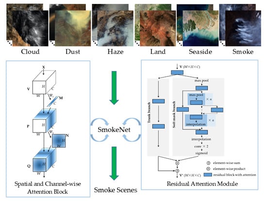
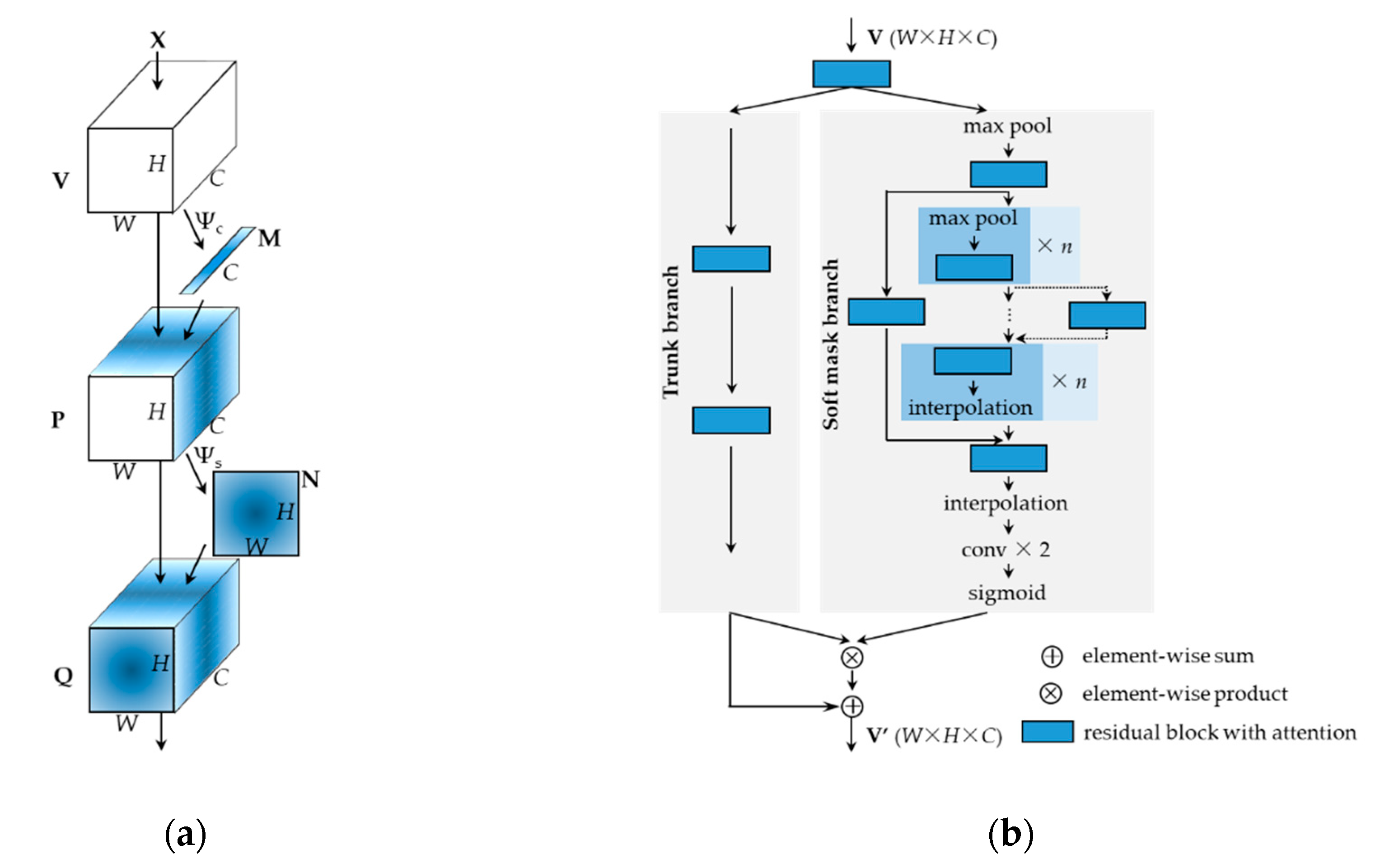
  • We improve the spatial attention mechanism in a deep learning network for scene classification. The SmokeNet model with spatial and channel-wise attention is proposed to identify the smoke scenes.
  • Experimental results on the new dataset show that the proposed model outperforms the state-of-the-art methods.
The remainder of this paper is organized as follows. Section 2 introduces the new dataset and the proposed model. Section 3 reports the experimental results. Section 4 provides the results analysis and discussion. Finally, Section 5 makes a few concluding remarks.

2. Materials and Methods

2.1. Dataset

2.1.1. Data Source

The data of the MODIS sensor mounted on Terra and Aqua satellites have been widely used for wildfire detection, monitoring, and assessment [3,6,13,50,51,52]. Since the launch of the Terra satellite in December 1999 [53] and the Aqua satellite in May 2002 [54], a large amount of MODIS data of wildfires has been captured during the past two decades. Besides, 38 spectral bands of the MODIS sensor covering from the visible to thermal infrared (TIR) domain can provide abundant spectral information for wildfire identification. Moreover, the MODIS sensor has four overpasses per day and a revisit of 1–2 days [50,55], which contributes to the monitoring of a wildfire development. Therefore, we select the MODIS data as our data source, and it can be acquired from our remote sensing platform located in Hefei, China and the Level-1 and Atmosphere Archive & Distribution System (LAADS) Distributed Active Archive Center (DAAC) located in the Goddard Space Flight Center in Greenbelt, Maryland, USA (https://ladsweb.nascom.nasa.gov/). The original MODIS Level 1B data were pre-processed in ENVI software by geometric correction to the universal transverse mercator (UTM) projection, and by radiometric calibration [56] to the data of reflectance and radiance. The MODIS bands 1, 4, and 3 can be used as the red, green, and blue channels to yield the true-color RGB images [10,14].

2.1.2. Classes

Taking into account the similar features of fire smoke in satellite imageries, we collected images of six wildfire-related scene classes based on MODIS data. The six classes are Cloud, Dust, Haze, Land, Seaside, and Smoke. The reasons for collecting these classes are listed as follows.
Smoke: Smoke is an important product in the development of a wildfire. It can quickly diffuse to a large scope, serving as a reliable signal for wildfire detection [57]. Therefore, we select smoke as the target class for wildfire detection. The images of smoke in different diffusion ranges are collected in the dataset. This contributes to the detection of the early stage of wildfires.
Dust/Haze: Dust and haze are considered as the negative classes to the smoke. In the practical application of fire detection, the similarity in texture and spectral characteristics of dust, haze, and smoke poses a huge challenge to the classification [58]. Besides, these large-scale disasters can overlap with various backgrounds, which brings challenges for their classification. Considering these difficulties, we include the images of dust and haze in our dataset.
Cloud: Cloud is the most common class in satellite imageries. It has the similar shape, color, and spectral features in comparison to smoke [6]. Meanwhile, smoke frequently mixes with cloud when wildfires occur. This makes it necessary to integrate the cloud images in our dataset.
Land/Seaside: As wildfires occur mainly on the land or near the seaside, these two classes are used as the backgrounds of fire smoke. Some land covers and geographic features, for example, the lakes illuminated by sunlight at certain angles, the bare soil of high reflectivity, the snow mountain, and the waves and sediments near the seaside, can also resemble the smoke. Moreover, land and seaside are the main classes in satellite imageries, which makes them essential for constructing the dataset.

2.1.3. Data Collection and Annotation

In order to construct the new smoke dataset, five students participated in the process of data collection and annotation. For scene classification, the image-level label was assigned to each image. The annotators were trained to collect the images of six classes according to the following criteria.
(1) We searched the wildfire, dust, and haze information all over the world in accordance with the historical news reporting by Google, Baidu, and other websites. The MODIS data of these disaster events span nearly twenty years and cover six continents except for Antarctica. The dust data were mainly obtained over the Middle East, Africa, and China, while the haze data mainly came from China and India. A large portion of smoke data was over North America, because of the frequent occurrence of large wildfires. Cloud and land images were also collected from these data. After the collection of MODIS data, the data pre-processing methods including geometric correction and radiometric calibration were performed to obtain the geometrically corrected reflectance and radiance data.
(2) On the basis of the information of the collected events (event type, time of occurrence, geographic location, and so on) and the spectral characteristics of these classes, we can determine the label for the events in the satellite imageries. The true-color and false-color composition RGB images were utilized together to identify fire smoke from other aerosol types, land, and seaside. For example, the true-color composition RGB image of MODIS bands 1, 4, and 3 can display both of the smoke and cloud [2,6], while the false-color composition RGB image of bands 7, 5, and 6 only displays the cloud as well as the post-fire area [50,59].
(3) The MODIS/Terra & Aqua Thermal Anomalies and Fire 5-Min L2 Swath 1 km products (MOD14/MYD14 products) were used to identify the wildfires, which can help us infer the location of fire smoke. In addition, according to the geographical location coordinates, the Google Earth software provides high-resolution satellite images, which can help determine the land cover types, for example, the lakes, snow mountains, and surfaces with high reflectivity. The product and software can provide meta information for our data collection and image label assignment.
(4) As long as there is fire smoke in the image, this image is labeled as the smoke class. The smoke, dust, and haze classes have the highest priority in the image label assignment. It is worth noting that the images of smoke, dust, and haze do not contain two other classes of this priority. This has been carefully checked in the annotation process to reduce the ambiguity between classes. However, the smoke, dust, and haze images may contain other classes such as cloud, land, or seaside, which is more in line with the real situation. In contrast, the secondary priority class in label assignment is the cloud and the lowest priorities are land and seaside.
(5) The true-color composition RGB images generated from MODIS bands 1, 4, and 3 were used to construct the new smoke dataset. The characteristics of MODIS bands 1, 3, and 4 are listed in Table 1. We used the dataset of true-color RGB images to develop our scene classification model because most optical satellite sensors can generate these RGB images compared with multispectral data. Also, this can ensure that the proposed model can be applied to the RGB images of other satellite sensors.

2.1.4. USTC_SmokeRS Dataset

The new dataset, namely USTC_SmokeRS, contains a total of 6225 RGB images from six classes: Cloud, Dust, Haze, Land, Seaside, and Smoke. Each image was saved as the “.tif” format with the size of 256 × 256 and the spatial resolution of 1 km. The number of images in each class is presented in Table 2, and the spatial distribution statistics of the images are presented in Figure 1. Moreover, Figure 2 shows some example images of these six classes in the dataset. The RGB dataset has been publicly released at https://pan.baidu.com/s/1GBOE6xRVzEBV92TrRMtfWg (password: 5dlk).

2.2. Method

Convolutional neural networks (CNNs) with the effective, scalable, and end-to-end learning structures have been widely used in scene classification [15,46]. Among these CNNs, ResNet with a residual learning framework is easy to optimize and can improve the accuracy of deep networks [35]. Besides, the attention mechanism brings a new momentum into the improvement of CNNs to exploit the most informative features. It has been demonstrated that the channel attention mechanism in the SE block [48] can effectively enhance the classification ability of the network. In addition, the spatial information is also very important for the scene classification task. In order to improve the classification results, the model should focus on the label-related regions rather than the irrelevant regions, for example, the background, in an image. On the basis of the structure design of the SE block, we further develop the spatial attention mechanism to enhance the network. This helps the model to make full use of the class-specific information for the scene classification.
Concretely, an input image X is transformed by the operations including convolution, pooling, and activation to obtain the output V = [ v 1 ,   v 2 ,   ,   v C ] , where v i is the i-th channel of the output V. Then, the attention mechanism is used for the output V to generate the spatial and channel-wise outputs Q and P. The structure illustration of the spatial and channel-wise attention is shown in Figure 3a, and the corresponding functions are defined as follows:
P = Ψ c ( V ) ,
Q = Ψ s ( V ) ,
where X ∈ ℝW×H×C, V ∈ ℝW×H×C, P ∈ ℝW×H×C, Q ∈ ℝW×H×C; C and C represent the total number of channels of input X and output V. W′ and W are the width of X and V, while H and H are the height of them. Functions Ψ c and Ψ s refer to the channel-wise and spatial attention, respectively.
In the process of channel-wise attention, we use the global average pooling for each channel of V to generate the channel feature Z = [ z 1 ,   z 2 ,   ,   z C ] , where z i is a statistical scalar of each channel. To obtain the channel-wise attention distribution M = [ m 1 ,   m 2 ,   ,   m C ] , we employ two fully connected layers with a sigmoid function, as done in the work of [48]. Finally, the distribution M is multiplied by V to generate the channel-wise attention output P   = [ p 1 ,   p 2 ,   ,   p C ] . The whole process can be defined as follows:
M = f 2 ( W 2 f 1 ( W 1 Z + b 1 ) + b 2 ) ,
p i = m i v i ,
where Z ∈ ℝC, M ∈ ℝC, W 1 ∈ ℝC/r×C, and W 2 ∈ ℝC×C/r are the weights; b 1   ∈ ℝC/r and b 2 ∈ ℝC are the biases; r is the reduction ratio, which is set to 16 following the parameter choice in the work of [48]; i indexes the channel number; and f 1 and f 2 denote ReLU and sigmoid activation function.
For the process of spatial attention, the transformation output V is firstly reshaped to U = [ u 1 ,   u 2 ,   ,   u l ] , where u j is the feature in the j-th location of each channel of V and l = W × H . Then, we also use two fully connected layers followed by a sigmoid function to obtain the spatial attention distribution N = [ n 1 ,   n 2 ,   ,   n C ] , where n i is the spatial attention distribution of v i . Finally, we multiply the distribution N by V to generate the spatial attention output Q = [ q 1 ,   q 2 ,   ,   q C ] . The whole process is formulated as follows:
N = f 2 ( W 2 f 1 ( W 1 U + b 1 ) + b 2 ) ,
q i = n i v i ,
where u j ∈ ℝC, N ∈ ℝW×H×C; and j indexes the location number. W 1 ∈ ℝC/r×C and W 2 ∈ ℝC×C/r are the weights. b 1 ∈ ℝC/r and b 2 ∈ ℝC are the biases, and r is set to 16.
In addition, we also integrate the residual attention modules (denoted as the RA module) [47] in our SmokeNet model to further exploit the discriminative information. The structure of the RA module is illustrated in Figure 3b. The output V ∈ ℝW×H×C of previous layers is processed by the RA module to generate V′ ∈ ℝW×H×C. The soft mask branch of the RA module uses the bottom-up top-down structure to generate the attention masks to improve the trunk branch features. Similar to the structure design of ResNet, the two-branch module adopts the residual attention learning to combine the outputs of soft mask branch and trunk branch. The criteria of residual attention learning is defined as follows:
O ( V ) = ( 1 + S ( V ) ) T ( V ) ,
where S(V), T(V), and O(V) represent the output of soft mask brunch, trunk branch, and RA module, respectively.
We also compared SmokeNet with two other effective models. The spatial and channel-wise attention ResNet (SCResNet) only utilizes the residual blocks with spatial and channel-wise attention in ResNet50 [35], whereas the channel-wise AttentionNet (CAttentionNet) incorporates the residual blocks only with channel-wise attention into the AttentionNet56 [47], which is stacked by RA modules. By integrating all the attention mechanisms, the proposed SmokeNet model, merging the residual blocks with spatial and channel-wise attention into AttentionNet56, can effectively improve the feature representation capacity for scene classification by using the most informative spatial information and channels of the intermediate feature maps. The overall structures of the SCResNet, CAttentionNet, and the proposed SmokeNet models are described in Table 3.

2.3. Implementation Details

The USTC_SmokeRS dataset (100%, 6225) was randomly divided into three subsets: training set (64%, 3984), validation set (16%, 999), and testing set (20%, 1242). In view of the difficulties in collecting disaster images, we investigated the performance of each model trained with four different proportions of training images: 16% (994), 32% (1988), 48% (2985), and 64% (3984). In these experiments, the validation and testing sets still use the same images and the proportions of 16% (999) and 20% (1242), respectively. The image sets for training, validation, and testing are listed in Table 4.
To fairly compare the performance of the state-of-the-art and proposed models, each model was trained, validated, and tested on the same images under the same experimental setting. Also, the initial parameters, optimization method, and loss function were identical for each model. Each model was trained on the training set and validated on the validation set. Afterwards, the trained parameters with the optimal validation accuracy were loaded to the model for the scene classification on the testing set. Specifically, training was carried out by the Adam method for stochastic optimization [61] with the weight decay (L2 penalty) set to 1 × 10⁻⁴. The loss function was the cross entropy loss. The learning rate was initially set to 0.001, and then decreased by the multiplication with a factor of 0.5 when the validation loss stopped decreasing. The batch size was set to 32, and maximum epochs to 200.
During the training phase, the input images with size of 256 × 256 were firstly resized to 230 × 230. Then, data augmentation with random image cropping to 224 × 224 and random horizontal and vertical flipping were employed. The resizing and cropping operations could ensure that the small regions/areas of smoke on the edge of the smoke images would not be removed. Afterwards, the input images were normalized with the mean and standard deviation value of 0.5. Through the experimental tests, these values can achieve better results than the values used in ImageNet images or the computed values for each channel in each image. During the validation and testing phases, the input images were directly resized to the size of 224 × 224 and processed by the normalization with the same mean and standard deviation values as used in the training phase.
All the experiments were conducted on the computer server with an E5-2630 CPU, two NVIDIA GeForce RTX 2080Ti GPUs with 11-GB memory. The operating system was Ubuntu 16.04 and the implementation framework was based on PyTorch [62] with CUDA toolkit.

2.4. Evaluation Protocols

We used the confusion matrix and evaluation metrics including testing accuracy, Kappa coefficient (K), omission error (OE), and commission error (CE) to quantitatively assess the model performance. The testing accuracy is computed by dividing the correctly classified testing images by the total number of testing images. OE is the ratio between the number of missing classified images of one class and the actual number of this class, while CE is calculated as the ratio between the number of one class falsely classified to other classes and the predicted number of this class [6]. Kappa coefficient (K) is frequently used in remote sensing for the assessment of accuracy and agreement degree [63,64]. In brief, the higher the accuracy and K, the lower the OE and CE, and the better the classification results. The confusion matrix example of t classes and the formulas of these evaluation metrics are shown in Table 5.
In order to reasonably explain the models’ decisions to predict the image class, we also employed the gradient-weighted class activation mapping (Grad-CAM) and the Guided Grad-CAM approaches [65] to generate the evaluating visualizations for the input images. The Grad-CAM approach was developed for the CNN-based models to coarsely highlight the discriminative regions in an image used to predict the image class. This technique can be combined with the guided backpropagation method [66], leading to the Guided Grad-CAM approach [65]. Guided Grad-CAM generates a high-resolution class-specific localization map, which can help us interpret the model prediction results. Therefore, the Grad-CAM and Guided Grad-CAM visualizations were utilized to qualitatively evaluate the model performance.

3. Results

3.1. Accuracy Assessment

On the basis of different proportions of training images from the USTC_SmokeRS dataset, we compared the performance of five state-of-the-art networks (VggNet-BN [33], ResNet [35], DenseNet [36], SE-ResNet [48], and AttentionNet [47]) with the proposed model (SmokeNet). In addition, we also evaluated the classification accuracy of two other models (SCResNet and CAttentionNet). The classification results of these eight models trained with four proportions (16%, 32%, 48%, and 64%) of training images are presented in Figure 4. The testing accuracy, K, OE, and CE comparisons are shown in Figure 4a–d, respectively. It can be found that the accuracy and K increase, while OE and CE decrease, as the number of training images increases. This is because more training images can help the models learn more robust features of each class. In addition, OE of the smoke scene detection of each model is higher than CE, which indicates that some smoke scenes are difficult to correctly recognize. This can be attributed to the similarity between the small regions/areas of smoke and the complex land covers. Furthermore, the proposed SmokeNet outperforms other models under different proportions/ratios of training images.
The testing accuracy, K value, and number of parameters of the eight models trained with 16% training images and the corresponding OE and CE of smoke class are listed in Table 6. It can be seen that the proposed SmokeNet outperforms other models with the accuracy of 85.10%, K of 0.8212, OE of 29.56%, and CE of 10.06% using the same 16% training images. The model improves the accuracy and K by at least 4.99% and 0.0600, respectively, over the state-of-the-art approaches. In addition, compared with the SE-ResNet50 model, SCResNet50 model also improves the accuracy by 3.14% and K by 0.0376, and decreases the OE by 7.88% and CE by 7.39% with a marginal increase (0.51 million) of network parameters. This demonstrates that the proposed spatial attention can effectively enhance the classification capacity of the network. Moreover, compared with the CAttentionNet56 model that combines the residual blocks only with channel-wise attention into AttentionNet56, the SmokeNet increases the accuracy and K value by 1.53% and 0.0184, respectively, while it also reduces the OE and CE by 1.47% and 11.73%, respectively. This further validates the efficacy of the proposed spatial attention mechanism for scene classification.
Table 7 shows the confusion matrix on testing set of the SmokeNet model trained with 64% training images. The results reveal that smoke scenes are prone to be confused with the dust, haze, and land images, as there are 16 smoke scenes misclassified to the haze and land classes, while six dust scenes are misclassified to the smoke class. This is because the dust and haze classes have similar shape and color with the widely spreading smoke under specific conditions such as illumination, wind, and so on [58]. Meanwhile, it is difficult to detect some small regions/areas of smoke emitted from the early stage of wildfire as a result of the similarities with highly reflective surfaces, lakes, or snow mountains in the land images, which caused the misclassification of smoke scenes to the land class. In addition, the dust and haze classes can be easily misclassified to each other as both of them are large-scale disasters with similar features of texture and color. These similarities among the smoke, dust, haze, and land classes further emphasize the significance to integrate them into the new dataset, making the dataset more challenging and practical for real-world application.

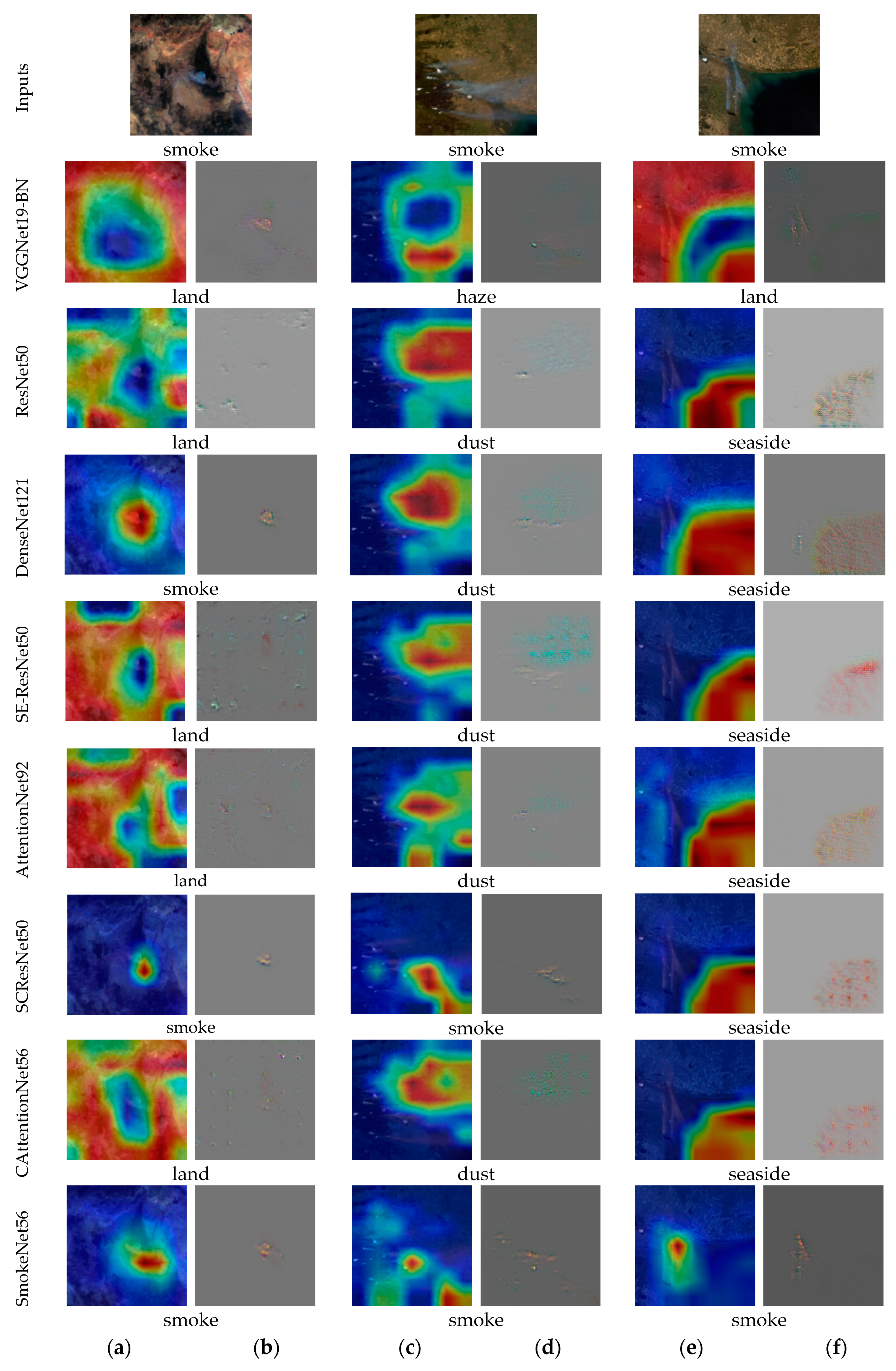
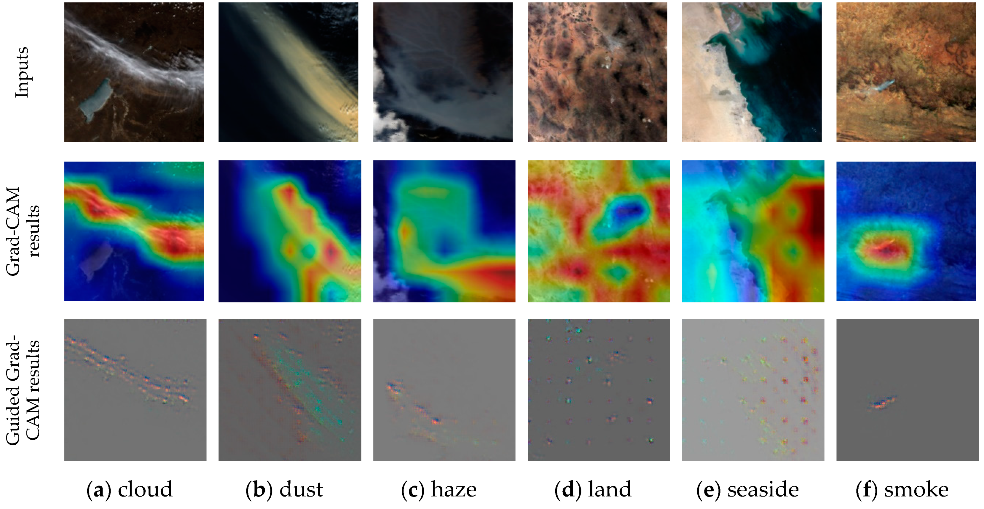
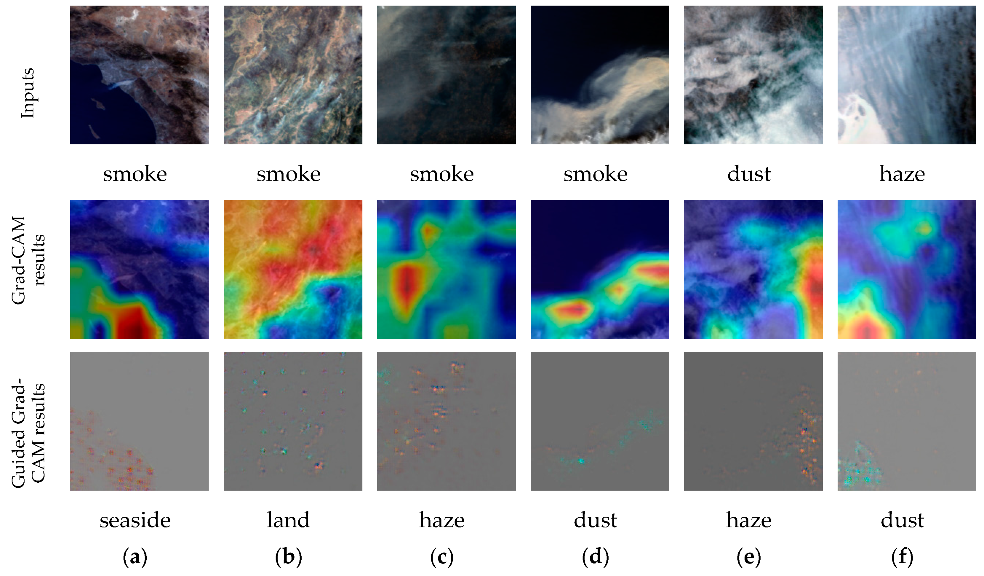
3.2. Visualization Analysis

The Grad-CAM and Guided Grad-CAM approaches were used to generate the evaluating visualizations for the input images to explain the models’ decision for scene classification. Figure 5 shows the comparison results of Grad-CAM and Guided Grad-CAM visualizations (presented in the second row to the last row) for three input smoke images (shown in the first row) based on eight models trained with 16% training images. The image classes predicted by these models for the three smoke images are displayed below the visualization results in each row. From the visualization results, it can be seen that the models, except for SmokeNet56 and SCResNet50, can only focus on the main features in an image, such as the texture and color of land, coastline, and water, which makes the small regions/areas of smoke difficult to detect using these models. In contrast, the SmokeNet56 and SCResNet50 models can utilize the class-discriminative features to correctly identify the class of smoke scenes. This illustrates that the proposed spatial attention improves the spatial-awareness capacity of networks for the discrimination of small regions/areas of smoke. On the basis of the visualization comparisons in the last three rows, the visualizations of SmokeNet56 model present more and fine-grained details of smoke over those of SCResNet50 and CAttentionNet56 models. Also, the Guided Grad-CAM results for SmokeNet56 model in Figure 5b,d,f columns can locate multiple smoke areas in comparison with the two other models. This demonstrates that the spatial, channel-wise attention, and RA modules integrated in the SmokeNet56 model contribute to the effective discrimination and accurate localization of multiple small smoke regions.
We also used the Grad-CAM and Guided Grad-CAM approaches to visualize the important regions that support the SmokeNet56 model to predict different classes, as shown in Figure 6. The model parameters were trained with 64% training images. The example images of six classes in the first row were correctly classified using the trained model. The second and third rows present the Grad-CAM and Guided Grad-CAM visualizations for each image. The important regions highlighted in red in the Grad-CAM visualizations reveal that the SmokeNet can use the most informative features to correctly identify the class in an image. Besides, the Guided Grad-CAM visualizations can display finer details of localization, shape, and texture of cloud, dust, haze, and smoke classes. For land and seaside images, the model can use the valid features in the whole image to determine their classes. On the basis of the qualitative analysis from the evaluating visualizations, it is thus believed that the proposed SmokeNet model integrating the spatial, channel-wise attention, and RA modules can effectively capture the class-discriminative features, so as to improve the classification results.
Figure 7 shows a few failure predictions and the corresponding visualizations of the SmokeNet model trained with 64% training images. The first row presents the input images and their actual labels, while the remaining rows show the Grad-CAM and Guided Grad-CAM visualizations and the predicted classes. From the evaluating visualizations, it can be seen that the small regions/areas of smoke emitted at the beginning of wildfire are very similar to some land surfaces in texture and color, as shown in Figure 7a,b. This means the model can only focus on the main features in the image. In contrast, when the smoke spreads over a wide area, it is difficult to distinguish it from the large-scale disasters such as haze and dust, which leads to the failures in the prediction for Figure 7c,d. Also, these similarities bring challenges for the discrimination between the haze and dust images in Figure 7e,f. Moreover, the overlaps of different classes, for example, haze and water at the bottom left of Figure 7f, can confuse the model.

4. Discussion

The classification results and evaluating visualizations indicate that the proposed SmokeNet model can achieve higher accuracy than the state-of-the-art models for scene classification on the USTC_SmokeRS dataset. For the purpose of remote sensing-based wildfire detection, we tried our best to collect thousands of satellite imageries of fire smoke and five smoke-related classes. This can solve the dilemma of lacking wildfire-related dataset. Meanwhile, the proposed SmokeNet has the advantage of integrating spatial channel-wise attention [48] and residual attention modules [47] to fully exploit the spatial class-discriminative features. The new dataset and model can effectively assist the identification of wildfire smoke, dust, and haze using satellite remote sensing.
In order to achieve the prompt detection of wildfire, we focus on the identification for the important wildfire signal, that is, smoke [57]. As mentioned in the works of [18,22], scene classification can automatically interpret an image with a specific class. From this point of view, unlike the previous smoke detection research [2,4,6,10,14], this paper aims to recognize the images containing the wildfire smoke, which is of critical importance to the rapid wildfire detection. However, existing aerial datasets for scene classification mainly concentrate on the specific land-use types, as shown in the works of [19,20,21,22], while the smoke-related datasets [23,24,25,26,27,28,29,30] were collected from the conventional cameras with close observation. These datasets cannot meet the demand of our task. This prompts us to delve into the long-term process of disaster data collection and processing. Optical satellite sensors may cover multi- and hyper-spectral domain [17], whereas the true-color RGB images generated from the visible spectral domain of red, green, and blue are commonly used for visual interpretation [6,7,14]. To ensure the applicability of the proposed model in different satellite sensors, RGB images were used instead of multispectral data to develop the smoke detection algorithm. In the future, we can also explore the use of CNN pre-trained parameters trained on large-scale RGB datasets to further improve the classification results of this task, which proves to be effective in the works of [33,67,68]. Therefore, we constructed the USTC_SmokeRS dataset with the true-color MODIS RGB images.
On the basis of the practical situation of fire smoke detection and the actual classes in the satellite imageries, we integrated more smoke-like aerosol classes and land covers in this new dataset, for example, cloud, dust, haze, bright surfaces, lakes, seaside, vegetation, and so on. This is an important improvement in comparison with the previous research [2,6,14], which considered only a few specific classes. Although this increases the difficulty of classification, it is very important for practical smoke detection. It is also worth noting that the images of each class contain a variety of land covers despite that there are six classes in the dataset. For example, the images of land class may consist of different classes of vegetation, surfaces, lakes, or mountains. The high inter-class similarities and small intra-class variations of the dataset make it more challenging to effectively distinguish the smoke scenes from other classes.
Uncertainties, Errors, and Accuracies: The effectiveness of the state-of-the-art and proposed models were validated on the new dataset. Given that the disaster images are more difficult to obtain as compared with the ordinary land-use types, we set up the experimental protocols with four different proportions of training images as described in Section 2.3. The experimental results illustrate that the proposed SmokeNet model outperforms other models trained with different numbers of training images. This is because SmokeNet can not only dynamically recalibrate the channel-wise features and generate the attention-aware features, but also optimize the representation of spatial information using the proposed spatial attention mechanism. The advantages were confirmed by the results in Figure 4 and Table 6. This refinement can effectively boost the spatial-aware capacity of network so as to take advantage of the class-specific features in an image for scene classification. To verify this statement, we also show the attention visualizations of different models in Figure 5 and Figure 6. Moreover, the proposed SmokeNet can process and identify around 20 images per second with a GeForce RTX 2080Ti GPU, which ensures the recognition speed of fire smoke in practical application. In this paper, the spatially explicit tests were not performed, but the spatial differences can be further explored in future work using the images divided according to the specific geographic regions.
In summary, the proposed SmokeNet demonstrated better capacity for smoke scene detection by merging the spatial and channel-wise attention. The new dataset collected in this study is also instrumental for researchers and practitioners working in the field of wildfire detection and remote sensing. In addition to the MODIS data, the proposed method has promising application prospects to identify fire smoke in the RGB images of other satellite sensors, such as the Advanced Himawari Imager (AHI) data of Himawari-8 satellite, Operational Land Imager (OLI) data of Landsat-8 satellite, Visible Infrared Imaging Radiometer Suite (VIIRS) data of Suomi National Polar-orbiting Partnership (S-NPP) satellite, Geostationary Operational Environmental Satellite (GOES) data, Sentinel satellite data, and GaoFen-4 (GF-4) satellite data, among others. As the satellite spatial resolution influences the range of smoke and land cover features in an image when the satellite data are processed into the true-color RGB images, the transfer learning among the satellite RGB images with different spatial resolutions is worth further exploration. In the future, we will assess the effectiveness of our model in the application of various satellite RGB images with different spatial resolutions. In addition, considering of the abundant spectral bands in satellite sensors, we will develop new algorithms that can utilize multispectral data and RGB images simultaneously to solve the difficulties discussed in Figure 7, thereby improving the classification results. Furthermore, the pixel-level smoke dataset will be constructed to help develop the model for the discrimination of smoke pixels and spreading areas in an image.

5. Conclusions

We propose a new CNN-based method to detect the smoke scenes using satellite remote sensing. As a result of the complex aerosol and land cover types in satellite imagery, taking only a few specific classes into account for algorithm development reduces the discrimination accuracy in practical smoke detection. Therefore, we constructed a new satellite imagery smoke dataset (USTC_SmokeRS) consisting of RGB images from more fire-related disasters and more complex land covers. Also, we developed the SmokeNet model merging the spatial and channel-wise attention, which can fully exploit the class-discriminative features for scene classification. To validate the model performance, we compared the proposed model with the state-of-the-art approaches on the new dataset. The experimental results indicate that our model can achieve higher accuracy and Kappa coefficient, as well as lower omission and commission error than the baseline models. The SmokeNet achieves the best accuracy of 92.75% and Kappa coefficient of 0.9130 using 64% training images. It also improves the accuracy and Kappa coefficient by at least 4.99% and 0.0600, respectively, and decreases omission and commission error by at least 1.47% and 5.52%, respectively, using 16% training images. The analysis also demonstrates that the proposed model with the spatial-aware and channel-wise attention is able to capture the most informative information in images for smoke scene detection.
Future research will be devoted to the model application in more satellite imageries with different spatial resolutions, and the utilization of multispectral data for smoke detection.

Author Contributions

Conceptualization, R.B. and W.S.; methodology, R.B., J.Y., and C.C.; software, R.B. and J.Y.; validation, R.B. and C.C.; formal analysis, C.C. and W.S.; investigation, R.B. and J.Y.; resources, W.S. and S.L.; data curation, R.B. and W.S.; writing—original draft preparation, R.B.; writing—review and editing, C.C., W.S., and S.L.; visualization, C.C. and R.B.; supervision, W.S., S.L., and C.C.; funding acquisition, W.S. and S.L.

Funding

This research was funded by National Key R&D Program of China, grant number 2018YFC0807000; the Research Grants Council, University Grants Committee of the Hong Kong Special Administrative Region (Project No. CityU 11300815); and the Fundamental Research Funds for the Central Universities, grant number WK6030000105.

Acknowledgments

The authors are grateful for the websites used to collect disaster information and the utilization of MODIS Level 1B data from Level-1 and Atmosphere Archive & Distribution System (LAADS) Distributed Active Archive Center (DAAC), located in the Goddard Space Flight Center in Greenbelt, Maryland (https://ladsweb.nascom.nasa.gov/).

Conflicts of Interest

The authors declare no conflict of interest.

Abbreviations

The following abbreviations are used in this paper:
MODISModerate Resolution Imaging Spectroradiometer
AVHRRAdvanced Very High Resolution Radiometer
BTbrightness temperature
BOVWbag-of-visual-words
SIFTscale invariant feature transform
DBNdeep belief network
SAsparse autoencoder
CNNconvolutional neural network
SEsqueeze-and-excitation
TIRthermal infrared
LAADSLevel-1 and Atmosphere Archive & Distribution System
DAACDistributed Active Archive Center
UTMUniversal Transverse Mercator
RA moduleresidual attention module
OEomission error
CEcommission error
KKappa coefficient
Grad-CAMGradient-weighted Class Activation Mapping
AHIAdvanced Himawari Imager
OLIOperational Land Imager
VIIRSVisible Infrared Imaging Radiometer Suite
S-NPPSuomi National Polar-orbiting Partnership
GOESGeostationary Operational Environmental Satellite
GFGaoFen

Websites

The following websites were used in the collection of the new dataset:
Google searchhttps://www.google.com/
Baidu searchhttps://www.baidu.com/
NASA Visible Earthhttps://visibleearth.nasa.gov/
NASA Earth Observatoryhttps://earthobservatory.nasa.gov/
Monitoring Trends in Burn Severity (MTBS)https://www.mtbs.gov/
Geospatial Multi-Agency Coordination (GeoMAC)https://www.geomac.gov/
Incident Information System (InciWeb)https://inciweb.nwcg.gov/
China Forest and Grassland Fire Preventionhttp://www.slfh.gov.cn/
DigitalGlobe Bloghttp://blog.digitalglobe.com/
California Forestry and Fire Protectionhttp://www.calfire.ca.gov/
MyFireWatch—Bushfire map information Australiahttps://myfirewatch.landgate.wa.gov.au/
World Air Quality Index Sitemaphttps://aqicn.org/

References

  1. Ryu, J.-H.; Han, K.-S.; Hong, S.; Park, N.-W.; Lee, Y.-W.; Cho, J. Satellite-Based Evaluation of the Post-Fire Recovery Process from the Worst Forest Fire Case in South Korea. Remote Sens. 2018, 10, 918. [Google Scholar] [CrossRef]
  2. Li, Z.Q.; Khananian, A.; Fraser, R.H.; Cihlar, J. Automatic detection of fire smoke using artificial neural networks and threshold approaches applied to AVHRR imagery. IEEE T. Geosci. Remote Sens. 2001, 39, 1859–1870. [Google Scholar] [Green Version]
  3. Zhao, T.X.-P.; Ackerman, S.; Guo, W. Dust and smoke detection for multi-channel imagers. Remote Sens. 2010, 2, 2347–2368. [Google Scholar] [CrossRef]
  4. Chrysoulakis, N.; Herlin, I.; Prastacos, P.; Yahia, H.; Grazzini, J.; Cartalis, C. An improved algorithm for the detection of plumes caused by natural or technological hazards using AVHRR imagery. Remote Sens. Environ. 2007, 108, 393–406. [Google Scholar] [CrossRef]
  5. Xie, Z.; Song, W.; Ba, R.; Li, X.; Xia, L. A Spatiotemporal Contextual Model for Forest Fire Detection Using Himawari-8 Satellite Data. Remote Sens. 2018, 10, 1992. [Google Scholar] [CrossRef]
  6. Li, X.L.; Song, W.G.; Lian, L.P.; Wei, X.G. Forest Fire Smoke Detection Using Back-Propagation Neural Network Based on MODIS Data. Remote Sens. 2015, 7, 4473–4498. [Google Scholar] [CrossRef] [Green Version]
  7. Chrysoulakis, N.; Opie, C. Using NOAA and FY imagery to track plumes caused by the 2003 bombing of Baghdad. Int. J. Remote Sens. 2004, 25, 5247–5254. [Google Scholar] [CrossRef]
  8. Randriambelo, T.; Baldy, S.; Bessafi, M.; Petit, M.; Despinoy, M. An improved detection and characterization of active fires and smoke plumes in south-eastern Africa and Madagascar. Int. J. Remote Sens. 1998, 19, 2623–2638. [Google Scholar] [CrossRef]
  9. Kaufman, Y.J.; Setzer, A.; Justice, C.; Tucker, C.; Pereira, M.; Fung, I. Remote sensing of biomass burning in the tropics. In Fire in the Tropical Biota; Springer: Berlin/Heidelberg, Germany, 1990; pp. 371–399. [Google Scholar]
  10. Xie, Y.; Qu, J.J.; Xiong, X.; Hao, X.; Che, N.; Sommers, W. Smoke plume detection in the eastern United States using MODIS. Int. J. Remote Sens. 2007, 28, 2367–2374. [Google Scholar] [CrossRef]
  11. Giglio, L.; Descloitres, J.; Justice, C.O.; Kaufman, Y.J. An Enhanced Contextual Fire Detection Algorithm for MODIS. Remote Sens. Environ. 2003, 87, 273–282. [Google Scholar] [CrossRef]
  12. Xie, Y.; Qu, J.; Hao, X.; Xiong, J.; Che, N. Smoke plume detecting using MODIS measurements in eastern United States. In Proceedings of the EastFIRE Conference, Fairfax, VA, USA, 11–13 May 2005; pp. 11–13. [Google Scholar]
  13. Wang, W.T.; Qu, J.J.; Hao, X.J.; Liu, Y.Q.; Sommers, W.T. An improved algorithm for small and cool fire detection using MODIS data: A preliminary study in the southeastern United States. Remote Sens. Environ. 2007, 108, 163–170. [Google Scholar] [CrossRef]
  14. Li, X.L.; Wang, J.; Song, W.G.; Ma, J.; Telesca, L.; Zhang, Y.M. Automatic Smoke Detection in MODIS Satellite Data based on K-means Clustering and Fisher Linear Discrimination. Photogramm. Eng. Remote Sens. 2014, 80, 971–982. [Google Scholar] [CrossRef]
  15. LeCun, Y.; Bottou, L.; Bengio, Y.; Haffner, P. Gradient-based learning applied to document recognition. Proc. IEEE 1998, 86, 2278–2324. [Google Scholar] [CrossRef] [Green Version]
  16. Krizhevsky, A.; Sutskever, I.; Hinton, G.E. Imagenet classification with deep convolutional neural networks. In Proceedings of the Advances in Neural Information Processing Systems, Lake Tahoe, NV, USA, 3–6 December 2012; pp. 1097–1105. [Google Scholar]
  17. Zhu, X.X.; Tuia, D.; Mou, L.; Xia, G.-S.; Zhang, L.; Xu, F.; Fraundorfer, F. Deep learning in remote sensing: A comprehensive review and list of resources. IEEE Geosci. Remote Sens. Mag. 2017, 5, 8–36. [Google Scholar] [CrossRef]
  18. Zhang, L.; Zhang, L.; Du, B. Deep learning for remote sensing data: A technical tutorial on the state of the art. IEEE Geosci. Remote Sens. Mag. 2016, 4, 22–40. [Google Scholar] [CrossRef]
  19. Yang, Y.; Newsam, S. Bag-of-visual-words and spatial extensions for land-use classification. In Proceedings of the 18th SIGSPATIAL International Conference on Advances in Geographic Information Systems, San Jose, CA, USA, 3–5 November 2010; pp. 270–279. [Google Scholar]
  20. Xia, G.-S.; Yang, W.; Delon, J.; Gousseau, Y.; Sun, H.; Maître, H. Structural high-resolution satellite image indexing. In Proceedings of the ISPRS TC VII Symposium-100 Years ISPRS, Vienna, Austria, 5–7 July 2010; pp. 298–303. [Google Scholar]
  21. Zou, Q.; Ni, L.; Zhang, T.; Wang, Q. Deep learning based feature selection for remote sensing scene classification. IEEE Geosci. Remote Sens. Lett. 2015, 12, 2321–2325. [Google Scholar] [CrossRef]
  22. Xia, G.-S.; Hu, J.; Hu, F.; Shi, B.; Bai, X.; Zhong, Y.; Zhang, L.; Lu, X. AID: A benchmark data set for performance evaluation of aerial scene classification. IEEE T. Geosci. Remote Sens. 2017, 55, 3965–3981. [Google Scholar] [CrossRef]
  23. Yuan, F. Video-based smoke detection with histogram sequence of LBP and LBPV pyramids. Fire Saf. J. 2011, 46, 132–139. [Google Scholar] [CrossRef]
  24. Xu, G.; Zhang, Y.; Zhang, Q.; Lin, G.; Wang, J. Deep domain adaptation based video smoke detection using synthetic smoke images. Fire Saf. J. 2017, 93, 53–59. [Google Scholar] [CrossRef] [Green Version]
  25. Zhang, Q.-x.; Lin, G.-h.; Zhang, Y.-m.; Xu, G.; Wang, J.-j. Wildland forest fire smoke detection based on faster R-CNN using synthetic smoke images. Proc. Eng. 2018, 211, 441–446. [Google Scholar] [CrossRef]
  26. Xu, G.; Zhang, Q.; Liu, D.; Lin, G.; Wang, J.; Zhang, Y.J.I.A. Adversarial Adaptation From Synthesis to Reality in Fast Detector for Smoke Detection. IEEE Access 2019, 7, 29471–29483. [Google Scholar] [CrossRef]
  27. Lin, G.; Zhang, Y.; Zhang, Q.; Jia, Y.; Xu, G.; Wang, J. Smoke detection in video sequences based on dynamic texture using volume local binary patterns. KSII Trans. Internet Inf. Syst. 2017, 11, 5522–5536. [Google Scholar] [CrossRef]
  28. Toreyin, B.U. Computer Vision Based Fire Detection Software & Dataset. Available online: http://signal.ee.bilkent.edu.tr/VisiFire/ (accessed on 10 March 2019).
  29. Péteri, R.; Fazekas, S.; Huiskes, M.J. DynTex: A comprehensive database of dynamic textures. Patt. Recogn. Lett. 2010, 31, 1627–1632. [Google Scholar] [CrossRef]
  30. Bansal, R.; Pundir, A.S.; Raman, B. Dynamic Texture Using Deep Learning. In Proceedings of the TENCON 2017–2017 IEEE Region 10 Conference, Penang, Malaysia, 5–8 November 2017. [Google Scholar]
  31. Zhu, Q.; Zhong, Y.; Zhao, B.; Xia, G.-S.; Zhang, L. Bag-of-visual-words scene classifier with local and global features for high spatial resolution remote sensing imagery. IEEE Geosci. Remote Sens. Lett. 2016, 13, 747–751. [Google Scholar] [CrossRef]
  32. Zhang, F.; Du, B.; Zhang, L. Saliency-guided unsupervised feature learning for scene classification. IEEE Trans. Geosci. Remote Sens. 2015, 53, 2175–2184. [Google Scholar] [CrossRef]
  33. Simonyan, K.; Zisserman, A. Very deep convolutional networks for large-scale image recognition. arXiv 2014, arXiv:1409.1556. [Google Scholar]
  34. Szegedy, C.; Liu, W.; Jia, Y.; Sermanet, P.; Reed, S.; Anguelov, D.; Erhan, D.; Vanhoucke, V.; Rabinovich, A. Going deeper with convolutions. In Proceedings of the IEEE Conference on Computer Vision and Pattern Recognition, Boston, MA, USA, 7–12 June 2015; pp. 1–9. [Google Scholar]
  35. He, K.; Zhang, X.; Ren, S.; Sun, J. Deep residual learning for image recognition. In Proceedings of the IEEE Conference on Computer Vision and Pattern Recognition, Las Vegas, NV, USA, 27–30 June 2016; pp. 770–778. [Google Scholar]
  36. Huang, G.; Liu, Z.; Van Der Maaten, L.; Weinberger, K.Q. Densely connected convolutional networks. In Proceedings of the IEEE Conference on Computer Vision and Pattern Recognition, Honolulu, HI, USA, 21–26 June 2017; pp. 4700–4708. [Google Scholar]
  37. Russakovsky, O.; Deng, J.; Su, H.; Krause, J.; Satheesh, S.; Ma, S.; Huang, Z.; Karpathy, A.; Khosla, A.; Bernstein, M.; et al. ImageNet large scale visual recognition challenge. IJCV 2015, 115, 211–252. [Google Scholar] [CrossRef]
  38. Krizhevsky, A.; Hinton, G. Learning Multiple Layers of Features from Tiny Images; No. 4. Technical Report; University of Toronto: Toronto, ON, Canada, 2009; Volume 1. [Google Scholar]
  39. Itti, L.; Koch, C. Computational modelling of visual attention. Nat. Rev. 2001, 2, 194. [Google Scholar] [CrossRef] [PubMed]
  40. Mnih, V.; Heess, N.; Graves, A. Recurrent models of visual attention. In Proceedings of the Advances in Neural Information Processing Systems, Montreal, ON, Canada, 8–13 December 2014; pp. 2204–2212. [Google Scholar]
  41. Bahdanau, D.; Cho, K.; Bengio, Y.J. Neural machine translation by jointly learning to align and translate. arXiv 2014, arXiv:1409.0473. [Google Scholar]
  42. Ba, J.; Mnih, V.; Kavukcuoglu, K.J. Multiple object recognition with visual attention. arXiv 2014, arXiv:1412.7755. [Google Scholar]
  43. Xu, K.; Ba, J.; Kiros, R.; Cho, K.; Courville, A.; Salakhudinov, R.; Zemel, R.; Bengio, Y. Show, attend and tell: Neural image caption generation with visual attention. In Proceedings of the International Conference on Machine Learning, Lille, France, 6–11 July 2015; pp. 2048–2057. [Google Scholar]
  44. Chen, L.; Zhang, H.; Xiao, J.; Nie, L.; Shao, J.; Liu, W.; Chua, T.-S. Sca-cnn: Spatial and channel-wise attention in convolutional networks for image captioning. In Proceedings of the IEEE Conference on Computer Vision and Pattern Recognition, Honolulu, HI, USA, 21–26 July 2017; pp. 5659–5667. [Google Scholar]
  45. Miech, A.; Laptev, I.; Sivic, J. Learnable pooling with context gating for video classification. arXiv 2017, arXiv:1706.06905. [Google Scholar]
  46. Jaderberg, M.; Simonyan, K.; Zisserman, A. Spatial transformer networks. In Proceedings of the Advances in Neural Information Processing Systems, Montreal, ON, Canada, 7–12 December 2015; pp. 2017–2025. [Google Scholar]
  47. Wang, F.; Jiang, M.; Qian, C.; Yang, S.; Li, C.; Zhang, H.; Wang, X.; Tang, X. Residual attention network for image classification. In Proceedings of the IEEE Conference on Computer Vision and Pattern Recognition, Honululu, HI, USA, 21–26 July 2017; pp. 3156–3164. [Google Scholar]
  48. Hu, J.; Shen, L.; Sun, G. Squeeze-and-excitation networks. In Proceedings of the IEEE Conference on Computer Vision and Pattern Recognition, Salt Lake City, UT, USA, 18–22 June 2018; pp. 7132–7141. [Google Scholar]
  49. Newell, A.; Yang, K.; Deng, J. Stacked hourglass networks for human pose estimation. In Proceedings of the European Conference on Computer Vision, Amsterdam, The Netherlands, 11–14 October 2016; pp. 483–499. [Google Scholar]
  50. Ba, R.; Song, W.; Li, X.; Xie, Z.; Lo, S. Integration of Multiple Spectral Indices and a Neural Network for Burned Area Mapping Based on MODIS Data. Remote Sens. 2019, 11, 326. [Google Scholar] [CrossRef]
  51. Wang, J.; Song, W.; Wang, W.; Zhang, Y.; Liu, S. A new algorithm for forest fire smoke detection based on modis data in heilongjiang province. In Proceedings of the 2011 International Conference on Remote Sensing, Environment and Transportation Engineering (RSETE), Nanjing, China, 24–26 June 2011; pp. 5–8. [Google Scholar]
  52. Melchiorre, A.; Boschetti, L. Global Analysis of Burned Area Persistence Time with MODIS Data. Remote Sens. 2018, 10, 750. [Google Scholar] [CrossRef]
  53. Terra. The EOS Flagship. Available online: https://terra.nasa.gov/ (accessed on 4 May 2019).
  54. Aqua Earth-Observing Satellite Mission. Aqua Project Science. Available online: https://aqua.nasa.gov/ (accessed on 4 May 2019).
  55. Pagano, T.S.; Durham, R.M. Moderate resolution imaging spectroradiometer (MODIS). In Proceedings of the Sensor Systems for the Early Earth Observing System Platforms, Orlando, FL, USA, 25 August 1993; pp. 2–18. [Google Scholar]
  56. Axel, A.C. Burned Area Mapping of an Escaped Fire into Tropical Dry Forest in Western Madagascar Using Multi-Season Landsat OLI Data. Remote Sens. 2018, 10, 371. [Google Scholar] [CrossRef]
  57. Allison, R.S.; Johnston, J.M.; Craig, G.; Jennings, S. Airborne optical and thermal remote sensing for wildfire detection and monitoring. Sensors 2016, 16, 1310. [Google Scholar] [CrossRef] [PubMed]
  58. Su, Q.; Sun, L.; Di, M.; Liu, X.; Yang, Y. A method for the spectral analysis and identification of Fog, Haze and Dust storm using MODIS data. Atmos. Meas. Tech. Discuss. 2017, 2017, 1–20. [Google Scholar] [CrossRef]
  59. Li, R.R.; Kaufman, Y.J.; Hao, W.M.; Salmon, J.M.; Gao, B.C. A technique for detecting burn scars using MODIS data. IEEE Trans. Geosci. Remote 2004, 42, 1300–1308. [Google Scholar] [CrossRef]
  60. Continent. Wikipedia. Available online: https://en.wikipedia.org/wiki/Continent (accessed on 10 July 2019).
  61. Kingma, D.; Ba, J. Adam: A method for stochastic optimization. arXiv 2014, arXiv:1412.6980. [Google Scholar]
  62. Paszke, A.; Gross, S.; Chintala, S.; Chanan, G.; Yang, E.; DeVito, Z.; Lin, Z.; Desmaison, A.; Antiga, L.; Lerer, A. Automatic differentiation in pytorch. In Proceedings of the NIPS 2017 Autodiff Workshop: The Future of Gradient-based Machine Learning Software and Techniques, Long Beach, CA, USA, 9 December 2017. [Google Scholar]
  63. Stroppiana, D.; Azar, R.; Calo, F.; Pepe, A.; Imperatore, P.; Boschetti, M.; Silva, J.M.N.; Brivio, P.A.; Lanari, R. Integration of Optical and SAR Data for Burned Area Mapping in Mediterranean Regions. Remote Sens. 2015, 7, 1320–1345. [Google Scholar] [CrossRef] [Green Version]
  64. Yu, S.; Jia, S.; Xu, C. Convolutional neural networks for hyperspectral image classification. Neurocomputing 2017, 219, 88–98. [Google Scholar] [CrossRef]
  65. Selvaraju, R.R.; Cogswell, M.; Das, A.; Vedantam, R.; Parikh, D.; Batra, D. Grad-cam: Visual explanations from deep networks via gradient-based localization. In Proceedings of the IEEE International Conference on Computer Vision, Las Vegas, NV, USA, 26 June–1 July 2016; pp. 618–626. [Google Scholar]
  66. Springenberg, J.T.; Dosovitskiy, A.; Brox, T.; Riedmiller, M. Striving for simplicity: The all convolutional net. arXiv 2014, arXiv:1412.6806. [Google Scholar]
  67. Sultani, W.; Chen, C.; Shah, M. Real-World Anomaly Detection in Surveillance Videos. In Proceedings of the IEEE Conference on Computer Vision and Pattern Recognition, Salt Lake City, UT, USA, 18–22 June 2018; pp. 6479–6488. [Google Scholar]
  68. Hu, F.; Xia, G.-S.; Hu, J.; Zhang, L. Transferring deep convolutional neural networks for the scene classification of high-resolution remote sensing imagery. Remote Sens. 2015, 7, 14680–14707. [Google Scholar] [CrossRef]
Figure 1. Spatial distribution of six classes of images in the USTC_SmokeRS dataset. The statistics of geographic location of the images are based on the seven-continent model [60].
Remotesensing 11 01702 g001
Figure 2. Example images of the six classes in the USTC_SmokeRS dataset. The images in the first column to the sixth column belong to Cloud, Dust, Haze, Land, Seaside, and Smoke, respectively.
Remotesensing 11 01702 g002
Figure 3. Structure illustration of the spatial, channel-wise attention, and the residual attention module. (a) Spatial and channel-wise attention; (b) residual attention (RA) module, where n denotes the number of units (n ≥ 0), the dotted line is disconnected if n is 0 and 1, and is connected when n is larger than 1; the blue block is the residual block [35] with spatial or channel-wise attention.
Remotesensing 11 01702 g003
Figure 4. Classification results of the state-of-the-art models (VggNet19-BN, ResNet50, DenseNet121, SE-ResNet50, and AttentionNet92), the combined models (CAttentionNet56 and SCResNet50), and the proposed SmokeNet56 trained with four proportions (16%, 32%, 48%, and 64%) of training images. (a) Testing accuracy; (b) Kappa coefficient; (c) omission error (OE) of the smoke class; (d) commission error (CE) of the smoke class.
Remotesensing 11 01702 g004
Figure 5. Comparison of gradient-weighted class activation mapping (Grad-CAM) and Guided Grad-CAM visualizations for the eight models. The first row presents the input smoke images and the remaining rows show the visualizations for the models listed on the left. (a), (c), and (e) columns are the Grad-CAM results highlighting the important regions in red; (b), (d), and (f) columns are the high-resolution class-discriminative visualizations of Guided Grad-CAM. The image class predicted by each model is displayed below the visualizations.
Remotesensing 11 01702 g005
Figure 6. Visualizations for the example images from six classes. The first row shows the input images, and the second and third rows present the visualizations of Grad-CAM and Guided Crad-CAM approaches, respectively.
Remotesensing 11 01702 g006
Figure 7. Examples of some failure predictions and the corresponding evaluating visualizations. The first row shows the input images and their actual labels, the second and third rows present the Grad-CAM and guided Crad-CAM visualizations and the predicted classes.
Remotesensing 11 01702 g007
Table 1. Characteristics of MODIS spectral bands 1, 3, and 4.
Spectral BandsBandwidth (µm)Spectral DomainPrimary Application
10.620–0.670redLand/Cloud Boundaries
30.459–0.479blueLand/Cloud Properties
40.545–0.565green
Table 2. Number of images for each class in the USTC_SmokeRS Dataset.
ClassCloudDustHazeLandSeasideSmoke
Number116410091002102710071016
Table 3. Structure details of the SCResNet, CAttentionNet, and proposed SmokeNet models.
Output SizeSCResNetCAttentionNetSmokeNet
112 × 112conv, 7 × 7, 64, stride 2
56 × 56max pool, 3 × 3, stride 2
56 × 56 ( conv ,   1   ×   1 ,   64   conv ,   3   ×   3 ,   64 conv ,   1   ×   1 ,   256 2 fc ,   ( 16 ,   256 ) 2 fc ,   ( 16 ,   256 )   ) × 3 ( conv ,   1   ×   1 ,   64 conv ,   3   ×   3 ,   64 conv ,   1   ×   1 ,   256 2 fc ,   ( 16 ,   256 ) ) × 1
RA-C module1 1 × 1
( conv ,   1   ×   1 ,   64   conv ,   3   ×   3 ,   64 conv ,   1   ×   1 ,   256 2 fc ,   ( 16 ,   256 ) 2 fc ,   ( 16 ,   256 )   ) × 1
RA-SC module1 2 × 1
28 × 28 ( conv ,   1   ×   1 ,   128   conv ,   3   ×   3 ,   128 conv ,   1   ×   1 ,   512 2 fc ,   ( 32 ,   512 ) 2 fc ,   ( 32 ,   512 )   ) × 4 ( conv ,   1   ×   1 ,   128 conv ,   3   ×   3 ,   128 conv ,   1   ×   1 ,   512 2 fc ,   ( 32 ,   512 ) ) × 1
RA-C module2 × 1
( conv ,   1   ×   1 ,   128   conv ,   3   ×   3 ,   128 conv ,   1   ×   1 ,   512 2 fc ,   ( 32 ,   512 ) 2 fc ,   ( 32 ,   512 )   ) × 1
RA-SC module2 × 1
14 × 14 ( conv ,   1   ×   1 ,   256   conv ,   3   ×   3 ,   256 conv ,   1   ×   1 ,   1024 2 fc ,   ( 64 ,   1024 ) 2 fc ,   ( 64 ,   1024 )   ) × 6 ( conv ,   1   ×   1 ,   256 conv ,   3   ×   3 ,   256 conv ,   1   ×   1 ,   1024 2 fc ,   ( 64 ,   1024 ) ) × 1
RA-C module3 × 1
( conv ,   1   ×   1 ,   256   conv ,   3   ×   3 ,   256 conv , 1   ×   1 ,   1024 2 fc ,   ( 64 ,   1024 ) 2 fc ,   ( 64 ,   1024 )   ) × 1
RA-SC module3 × 1
7 × 7 ( conv ,   1   ×   1 ,   512   conv ,   3   ×   3 ,   512 conv ,   1   ×   1 ,   2048 2 fc ,   ( 128 ,   2048 ) 2 fc ,   ( 128 ,   2048 )   ) × 3 ( conv ,   1   ×   1 ,   512 conv ,   3   ×   3 ,   512 conv ,   1   ×   1 ,   2048 2 fc ,   ( 128 ,   2048 ) ) × 3 ( conv ,   1   ×   1 ,   512   conv ,   3   ×   3 ,   512 conv , 1   ×   1 ,   2048 2 fc ,   ( 128 ,   2048 ) 2 fc ,   ( 128 ,   2048 )   ) × 3
1 × 1global average poolaverage pool, 7 × 7, stride 1
fc, softmax, 6
1 RA-C module denotes the residual attention module using the residual block with the channel-wise attention. 2 RA-SC module denotes the residual attention module using the residual block with the spatial and channel-wise attention. n in RA module 1, 2, and 3 is set to 2, 1, and 0, respectively, which are the same as in the work of [47]. The operations, kernel size, and number of output channels are presented in the parentheses. fc represents one fully connected layer and the size of its output is shown after it. The number of the stacked units is outside the parentheses.
Table 4. Image sets for training, validation, and testing.
Image SetNumber of ImagesProportion
Training set99416%
198832%
298548%
398464%
Validation set99916%
Testing set124220%
USTC_SmokeRS6225100%
Table 5. Confusion matrix example of t classes and the formulas of accuracy, Kappa coefficient, omission error, and commission error.
ClassPredicted Class 1Predicted Class tOmission Error (OE)Commission Error (CE)
Actual Class 1N11N1t OE class 1 = N 1 + N 11 N 1 + CE class 1 = N + 1 N 11 N + 1
Actual Class tNt1Ntt OE class t = N t + N t t N t + CE class t = N + t N t t N + t
Accuracy Accuracy = 1 t N i i N
Kappa coefficient (K) K = N 1 t N i i 1 t ( N i + N + i ) N 2 1 t ( N i + N + i )
In this table, i denotes a certain class and t is the total number of classes; N represents the total number of images; Nii refers to the number of correctly classified images in the diagonal; and Ni+ and N+i are the sum of images in the i-th row and i-th column, respectively.
Table 6. Classification results of the eight models trained with 16% training images and the number of model parameters.
ModelLayersAccuracy (%)KOE (%)CE (%)Params (Million)
VGGNet-BN [33]1954.670.457287.6865.28143.68
ResNet [35]5073.510.682153.2036.6725.56
DenseNet [36]12178.100.737134.4831.797.98
AttentionNet [47]9277.860.734241.8732.1883.20
SE-ResNet [48]5080.110.761243.8422.9728.07
CAttentionNet5683.570.802831.0321.7950.57
SCResNet5083.250.798835.9615.5828.58
SmokeNet5685.100.821229.5610.0653.52
Table 7. Confusion matrix on testing set of the SmokeNet model trained with 64% training images.
ClassCloudDustHazeLandSeasideSmokeOE (%)CE (%)
Cloud227013012.162.99
Dust01741551613.4310.77
Haze0131833018.5013.68
Land443193015.859.39
Seaside002119711.991.50
Smoke3488217812.325.32
Accuracy92.75%
K0.9130

