Article

Comparing Deep Neural Networks, Ensemble Classifiers, and Support Vector Machine Algorithms for Object-Based Urban Land Use/Land Cover Classification

by
Shahab Eddin Jozdani
1,
Brian Alan Johnson
2 and
Dongmei Chen
1,*
1
Department of Geography and Planning, Queen’s University, Kingston, ON K7L 3N6, Canada
2
Natural Resources and Ecosystem Services Area, Institute for Global Environmental Strategies, 2108-1 Kamiyamaguchi, Hayama, Kanagawa 240-0115, Japan
*
Author to whom correspondence should be addressed.
Remote Sens. 2019, 11(14), 1713; https://0-doi-org.brum.beds.ac.uk/10.3390/rs11141713
Submission received: 10 June 2019 / Revised: 5 July 2019 / Accepted: 16 July 2019 / Published: 19 July 2019
(This article belongs to the Section Urban Remote Sensing)

Abstract

:
With the advent of high-spatial resolution (HSR) satellite imagery, urban land use/land cover (LULC) mapping has become one of the most popular applications in remote sensing. Due to the importance of context information (e.g., size/shape/texture) for classifying urban LULC features, Geographic Object-Based Image Analysis (GEOBIA) techniques are commonly employed for mapping urban areas. Regardless of adopting a pixel- or object-based framework, the selection of a suitable classifier is of critical importance for urban mapping. The popularity of deep learning (DL) (or deep neural networks (DNNs)) for image classification has recently skyrocketed, but it is still arguable if, or to what extent, DL methods can outperform other state-of-the art ensemble and/or Support Vector Machines (SVM) algorithms in the context of urban LULC classification using GEOBIA. In this study, we carried out an experimental comparison among different architectures of DNNs (i.e., regular deep multilayer perceptron (MLP), regular autoencoder (RAE), sparse, autoencoder (SAE), variational autoencoder (AE), convolutional neural networks (CNN)), common ensemble algorithms (Random Forests (RF), Bagging Trees (BT), Gradient Boosting Trees (GB), and Extreme Gradient Boosting (XGB)), and SVM to investigate their potential for urban mapping using a GEOBIA approach. We tested the classifiers on two RS images (with spatial resolutions of 30 cm and 50 cm). Based on our experiments, we drew three main conclusions: First, we found that the MLP model was the most accurate classifier. Second, unsupervised pretraining with the use of autoencoders led to no improvement in the classification result. In addition, the small difference in the classification accuracies of MLP from those of other models like SVM, GB, and XGB classifiers demonstrated that other state-of-the-art machine learning classifiers are still versatile enough to handle mapping of complex landscapes. Finally, the experiments showed that the integration of CNN and GEOBIA could not lead to more accurate results than the other classifiers applied.

1. Introduction

1.1. High Spatial Resolution Urban Mapping

Since the launch of IKONOS—the first commercial high-spatial resolution (HSR) spaceborne sensor—in 1999, much research has focused on developing new methods for analyzing HSR images (spatial resolution < 4 m). Undoubtedly, one of the most common applications of HSR remote sensing (RS) data is urban land use/land cover (LULC) mapping. Due to rapid changes in urban areas, maps must frequently be updated to support urban management and planning. Apart from the fine resolution of HSR imagery, its ability to provide ongoing and ad hoc monitoring is also beneficial for urban (change) mapping.
A major challenge in using HSR imagery for urban LULC mapping, however, is the high degree of complexity of urban features, e.g., in terms of their spectral, spatial, and textural properties [1]. For instance, different types of urban LULC features may have very similar spectral properties (e.g., buildings and road). Moreover, some urban LULC features like buildings have spectral and spatial properties that may vary widely even within a single urban area. Owing to these reasons, applying traditional pixel-wise approaches to classify urban LULC often leads to unsatisfactory results [2,3]. In fact, since a single pixel in an HSR image represents just a small part of an LULC object (e.g., building rooftop or tree crown), pixel-wise classification cannot properly model the variability of different LULC types. To put it differently, the lack of extra information (i.e., spectral, spatial, and textural) hinders pixel-wise classification schemes from correctly assigning individual pixels to their real-world land classes.
To overcome this problem, Geographic Object-Based Image Analysis (GEOBIA) was developed [4]. GEOBIA deals with the shortcomings of pixel-based approaches by including an additional step in the classification phase, known as image segmentation. The objective of image segmentation is to group pixels into semantically similar nonoverlapping regions from which additional spectral, spatial, and textural features can be extracted and used for classification. In contrast to pixel-based techniques, image segments (or image objects) are the smallest addressable element in the GEOBIA framework. These image segments are typically desired to accurately represent real-world, meaningful entities (although this can be difficult to achieve in practice). As shown in many previous studies, GEOBIA often leads to more accurate classification results than pixel-based approaches, particularly for HSR images [1,3,5,6].

1.2. Machine learning Classifiers for Object-Based Classification

Aside from the base units for classification (pixels or image segments), the selection of a suitable classifier is also of critical importance for urban LULC mapping. The success of machine learning (ML) algorithms in classification of highly complex data has substantially increased their applications for RS analysis, and indeed they have been found to significantly outperform parametric methods in many past RS studies [6,7].
A wide variety of ML classification techniques exist, with ensemble decision tree classifiers (e.g., Random Forest (RF), Bagging Trees (BT), Boosted Trees, etc.) [8,9] and Support Vector Machine (SVM) [10] being among the most commonly utilized for GEOBIA-based urban LULC classification [11]. More recently, algorithms employing deep learning (DL) (i.e., Deep Neural Networks (DNNs)) [12] have also become very popular for LULC classification [13]. Recently, several powerful architectures of DL models have been developed for the classification of RS images [14,15,16]. It is, however, still arguable how well these DL algorithms perform against ensemble algorithms and SVM for the purpose of urban LULC classification. This is particularly true in the case of LULC classification using a GEOBIA approach, as it can be difficult to combine GEOBIA with some popular DL algorithms, e.g., convolutional neural networks (CNNs) [17,18].
Recently, a few studies have explicitly targeted the comparison of DL and other common ML algorithms. In Liu, et al. [19], the aim was to show whether DL could outperform SVM for the classification of hyperspectral data. In this regard, a deep sparse autoencoder (SAE) [20]—one of the variants of DL algorithms—was applied against SVM. The authors concluded that SVM generally performed better than SAE in their experiments. Moreover, as they outlined, the best accuracies generated by SAE were close to those of SVM. In their study, however, the authors attributed the unexpected performance of SAE in comparison with SVM to the insufficient number of labeled samples in the hyperspectral data sets under consideration. İn a similar study, Zhang, et al. [21] implemented an object-based framework to compare DL (i.e., SAE and stacked denoising autoencoders (DAE) [22]) and common ML classifiers (i.e., SVM, K-nearest neighbors, and Bayes) for fine-scale urban mapping. They trained these algorithms on a 181-dimensioanl feature space (i.e., spectral features (including “brightness”, “mean”, “standard deviation”, “max/min pixel values”, etc.), spatial features (including “area”, “asymmetry”, “border index/length”, “compactness”, “elliptic fit”, etc.), and textural features (including “GLCM” and “GLDV”) to assess the capability of each algorithm in urban mapping using a high-dimensional data set. In contrast to the study conducted by Liu, et al. [19], Zhang, et al. [21] concluded that the DNNs achieved higher accuracies than SVM (by 6%) for urban mapping. They reported that their proposed DL framework was superior to the other classifiers evaluated. Fu, et al. [17] compared CNN with RF and SVM for the classification of urban LULC types using a GEOBIA approach, and found that CNN led to 5–10% increases in overall classification accuracy. However, because CNN classification features were extracted for fixed-sized square image blocks rather than segment boundaries (due to the limitations of CNNs in this regard), classification results tended to be erroneous if segments had curved or elongated shapes. A similar approach was applied by Liu and Abd-Elrahman [23]. The important difference in their approach was the use of multiview images taken by UAVs. In that method, after extracting the object from each image acquired from a specific angle, the image patch was incorporated into a CNN. The main advantage of this approach was that it accounts for spectral difference of the image objects, so that less training data are needed. However, this demands for multiview images and could be computationally intensive.

1.3. Objective

In spite of the novelty of the above-mentioned studies in comparing DL and other state-of-the-art ML classifiers for urban LULC mapping, to our knowledge, no comprehensive comparison with other commonly used ensemble learners (aside from RF) for fine-scale urban LULC mapping has been performed to better judge the potential of different DL architectures in urban mapping in a GEOBIA-based setup. There are several aspects that distinguish this study from other recent studies on comparing ML algorithms. First, we aimed to compare different types of ML algorithms that are reported to be mature in several studies [19,24,25,26,27]. Some of these algorithms, however, have not been comprehensively compared with each other. For example, although it is argued that RF is the most popular ensemble model for the classification of RS images [24], it has not been thoroughly experimentally compared with other (state-of-the-art) tree ensemble approaches in the context of LULC classification using the GEOBIA approach. Second, along with not applying other variants of autoencoders, the efficacy of applying a deep regular multilayer perceptron (MLP) model without performing any pretraining procedure or specific regularization has not been investigated. Moreover, in previous studies, the potential of an object-based CNN model against other object-based DL models was not evaluated to judge if the integration of CNN and GEOBIA can perform better than the other types of GEOBIA-based DNNs. Finally, we used a multiscale GEOBIA classification in our comparisons (except for the CNN). Notwithstanding that in several previous studies the importance of multiscale mapping has been shown [3,6,28], almost all the similar studies chose to use a single-scale comparison [19,25,27,29].
Taking into account these limitations, this study focused on the comparison of two popular variants of stacked autoencoders (i.e., SAE and variational autoencoders (VAE)), MLP, and CNN for GEOBIA LULC classification. In addition, the DNNs applied were compared with some of the most powerful ensemble tree classifiers (i.e., RF, BT, GB [30], and XGB [31]) as well as SVM to provide a comprehensive comparison.

2. Overview of Selected ML Classifiers

2.1. Ensemble Classifiers

A basic principle behind ensemble learning is that, by combining a series of classifiers that perform slightly better than random guessing (known as weak learners), a single strong classifier can be constructed. A decision tree (DT) classifier [32] is the epitome of a weak learner, and is often incorporated into ensembles to establish a strong classifier. One popular type of ensemble tree models is referred to as Bootstrap Aggregation, or Bagging Trees (BT) [33]. As with its other ensemble counterparts, the BT model aims to address the problem of overfitting of DTs. The BT model involves randomly selecting a subset of the training data (with replacement) to train each individual decision tree model in the ensemble. The final classification result is obtained through majority voting of the output (i.e., LULC class) of the individual DTs in the ensemble.
The RF classifier is similar to BT in that each DT in the ensemble is grown using a random subset of the training data, but RF also randomly selects a subset of the classification variables for classifying each DT [24]. The generated DTs thus have higher variance and lower bias. To train an RF model, two hyperparameters need to be set: the number of randomly selected features (Mtry) used for splitting each node and the number of trees (Ntree). Based on the experiments of Breiman [9], reasonable accuracy was obtained on different data sets when Mtry was set to log 2 ( M ) + 1 where M is the number of variables. In addition, Lawrence, et al. [34] reported that an Ntree of 500 or more produced unbiased estimates of error.
Boosting algorithms are greedy techniques that are also popular in the context of RS [26]. Unlike BT and RF, boosting models do not grow DTs in parallel. They instead sequentially train individual DTs, each of which is an improved version of the previous one that resulted in smaller error rate. The most commonly used type of boosting algorithms is perhaps Adaptive Boosting (AdaBoost) [35]. The foundation of boosting was later improved by introducing a more generalized solution called gradient boosting (GB) [36]. GB works based on minimizing a loss function through fitting an additive basis function model sequentially to the gradient residual of the loss function. Another improved version of the regular gradient tree boosting model recently proposed is XGB [31]. This type of ensemble tree models has been recently reported to be a powerful ML algorithm for mapping purposes in RS [37,38]. This algorithm is in fact a specific implementation of the concept of the regular GB. In XGB, a regularization term (added to the loss function) is used to constrain the model, thereby helping control the complexity of the model, better avoiding overfitting. To train an XGB model, three main parameters should be set: Ntree, learning rate (eta), and the depth of each individual tree (depth). Tuning these three free parameters helps improve the performance of the model in terms of both speed and accuracy.

2.2. Support Vector Machines (SVM)

SVM is one of the most commonly used classifiers in the ML community that categorizes data using an optimally separating hyperplane [10]. One key advantage of SVM for RS applications is its ability to handle high dimensionality data using relatively few training samples [39]. However, in cases where the number of features is much greater than the number of training samples, which is the so-called curse of dimensionality, this classifier fails to generate acceptable results. In general, a radial basis function (rbf) is used as the kernel for this classifier because it provides a trade-off between time-efficiency and accuracy [40]. This classifier has two free parameters that need to be tuned, namely C (penalty parameter of the error term) and ε (the margin of tolerance). These two parameters are typically selected by cross-validation of the training samples and grid-search.

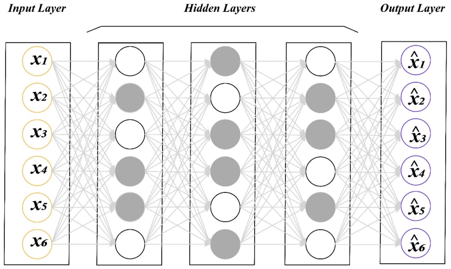
2.3. Deep Learning Architectures

The structure of an MLP, which is of the family of feedforward networks, can be schematically seen in Appendix A (Figure A1). An MLP is composed of four main components: Input layer, neurons (nodes), hidden layers, and output layer. To put it simply, an MLP can be defined as a series of layers of neurons successively connected to each other by weights, which are iteratively adjusted through an optimization process. The training procedure in feedforward neural networks is based on the back-propagation algorithm. This algorithm propagates error from the output layer to the input layer. Through this process, which usually employs stochastic gradient descent approach for optimizing the loss function, the weights in each layer of the network are updated iteratively until network’s error rate reaches a desired minimum state.
In the earlier forms of feedforward networks, adding more than one layer to the network did not have any effect on the accuracy. In fact, the gradient update was not able to back-propagate the error to the first layers, and thus no parameter update was applied to them; this phenomenon, known as vanishing gradients, was one of the main barriers to applying DNNs. In one of the revolutionary findings by Glorot and Bengio [41] in the field of neural networks, this problem was overcome using a new strategy for weight initialization. This provided new insights into taking advantage of DNNs to model complex patterns in different applications including object detection/recognition, semantic segmentation, hand-written recognition, speech recognition, etc.
Although the number of hidden layers and neurons can affect the performance of a network, there is not any solid rule for determining optimal values for them. It is also obvious that fitting more complex models (by designing more complex DNNs) to the input data increases the possibility of overfitting. To address this problem, these two hyperparameters can be set by performing cross-validation or based on a user’s a priori knowledge. In addition, to overcome overfitting, regularization techniques, including dropout, are normally applied to increase the generalizability of the model.
Autoencoders are a variant of neural networks that are structurally similar to MLPs. The main application of an autoencoder is to find the features that best represent input data reconstructed, helping prevent overfitting, especially in cases where sufficient labeled data are not available [42]. Therefore, they could be very useful in RS applications because of the difficulty in collecting labeled data. As seen in Figure A2, an autoencoder has two main parts that distinguish it from an MLP, namely the coding layer and decoding layer. In the coding layer, the network learns to map the data to a lower-dimensional feature space, similar to what Principal Component Analysis (PCA) does.
The decoding layer is responsible for reconstructing the coded, dimensionally reduced data. To put it differently, this layer approximates the input data using the coded data. It is therefore evident that the number of neurons in the input layer must be the same as the number of neurons in the output layer. To reconstruct complex data more accurately, it is possible to stack multiple autoencoders together, resulting in a deep autoencoder or stacked autoencoder. The coding layers of a stacked autoencoder can also be fed into a supervised learning model for classification purposes.
Explicitly reducing the number of neurons that our output from the encoding layer is not the only solution to reduce dimensionality and to extract useful structures from the input data in an unsupervised setup. Penalizing the neurons of a stacked autoencoder is another way to compress feature space, which permits the same or more neurons in successive layers as their input features. In this regard, one solution is to add a sparsity term to the loss function to establish SAE (Figure A3). To put it simply, by adding this sparsity term during training process, some neurons in the coding layer are deactivated to preclude the model from memorizing the pattern/structure of training data. Sparsifying the network at each training iteration helps the network learn more useful features to reconstruct the input data even when a larger number of neurons in the hidden layers are used. The sparsity term commonly used is Kullback–Leibler (KL) divergence, which is a function for comparing the similarity between two distributions. This extra term added to the loss function has two free parameters: sparsity parameter and sparsity weight. The sparsity parameter controls the average activation of hidden neurons (i.e., neurons in the hidden layer(s)). The sparsity weight is a scale value that determines the magnitude of the sparsity term imposed.
Another powerful type of autoencoders is variational autoencoder (VAE) [43]. Unlike regular autoencoders and SAEs, a VAE is a probabilistic model; that is, a VAE maps the input data to a probability distribution (in the coding space or latent space) rather than to a fixed encoded vector. Instead of learning a function to map a single data point in the feature space into an encoded single value, a VAE learns the parameters (i.e., mean and standard deviation) of a probability distribution (in a latent space) from the input data. From this probability distribution, which is typically chosen (but not limited) to be Gaussian, a single data point is randomly sampled through an additional layer called sampling layer. Finally, the samples are fed into the decoding layer to apply the reconstruction process. A VAE also takes advantage of the KL divergence for comparing the distribution learned with a normal distribution (with a mean of 0 and standard deviation of 1). In other words, the KL divergence controls if the learned distribution is not significantly different from a normal distribution (For more detailed information on VAEs, the reader is recommended to refer to Doersch [44]). As implied from the above descriptions, VAEs are inherently generative models. Indeed, the capability of VAEs in transforming input data to a probability distribution and then sampling from it helps them be able to generate new instances from the probability distribution constructed. This feature is useful in cases where sufficient labeled data are not available for classification so that the analyst can use a VAE to synthesize new instances to improve the accuracy and generalizability of modeling.
Another variant of feedforward multilayer models is CNN, which is perhaps currently the most popular DL model for object detection/identification. CNNs are very simplistic analogies of the mammalian visual cortex. Unlike MLP and autoencoders, inputs into CNNs are image patches, not vectorized data, which is very useful for extracting/learning spatial and contextual features. In a CNN architecture, a fixed-size image patch is mapped to a vector of probabilities calculated for each of the classes considered [42]. Another difference between an MLP and a CNN is that CNNs are not fully connected (except their last layer), which means that each neuron is not connected to all other neurons in the next layer. In fact, this is the main advantage of CNNs that helps them generate learned features through applying sequentially convolutional filters to fixed-size inputs. In the first layers, convolutional filters extract low-level features (e.g., edges). The last layers, on the other hand, are responsible for extracting and learning high-level information (e.g., land features). When stacked together, these convolutional layers can be very beneficial to detect/recognize objects of interest. To improve the efficiency of CNNs, some convolutional layers are followed by a pooling/subsampling layer to reduce output size of the convolutional layers. One of the problems with CNNs is that they only accept fixed-size image patches. In RS mapping, this can negatively affect classification results because LULC boundaries for geometrically distorted and for small LULCs can be ignored by the convolutional filters used in the CNN, which causes unwanted uncertainty in the classification process [29]. One of the solutions to address this problem is to integrate GEOBIA with a CNN to account for the boundaries of land features to be classified.

3. Methods and Materials

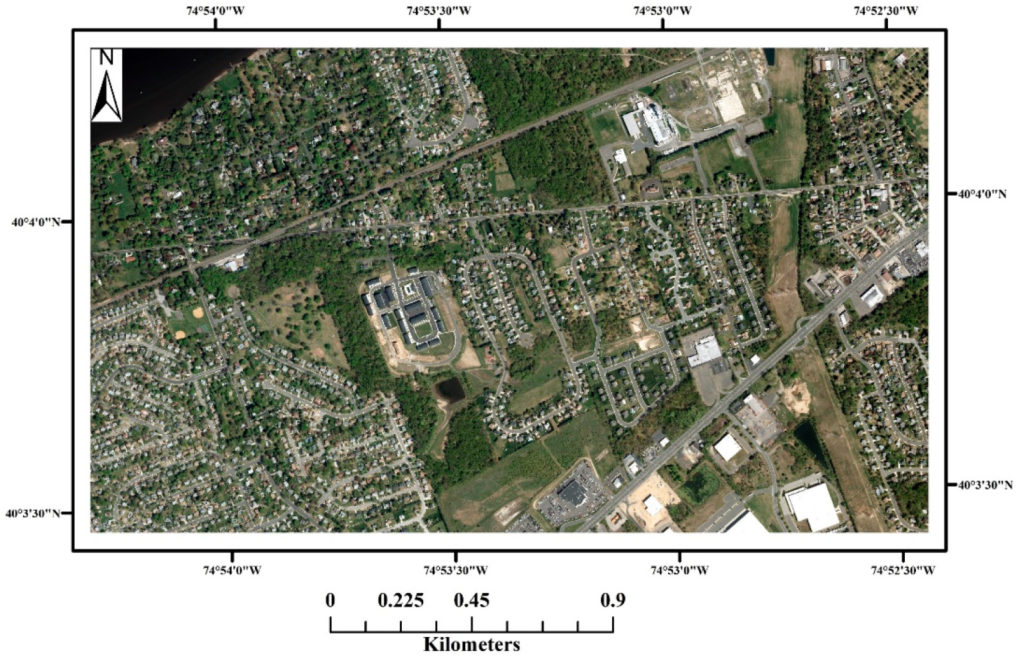
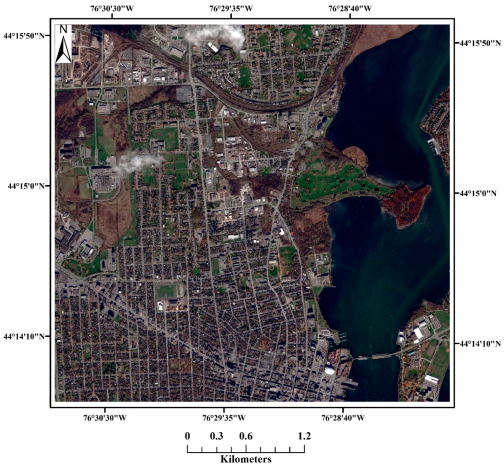
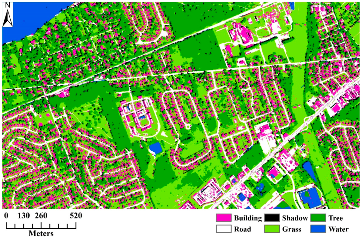
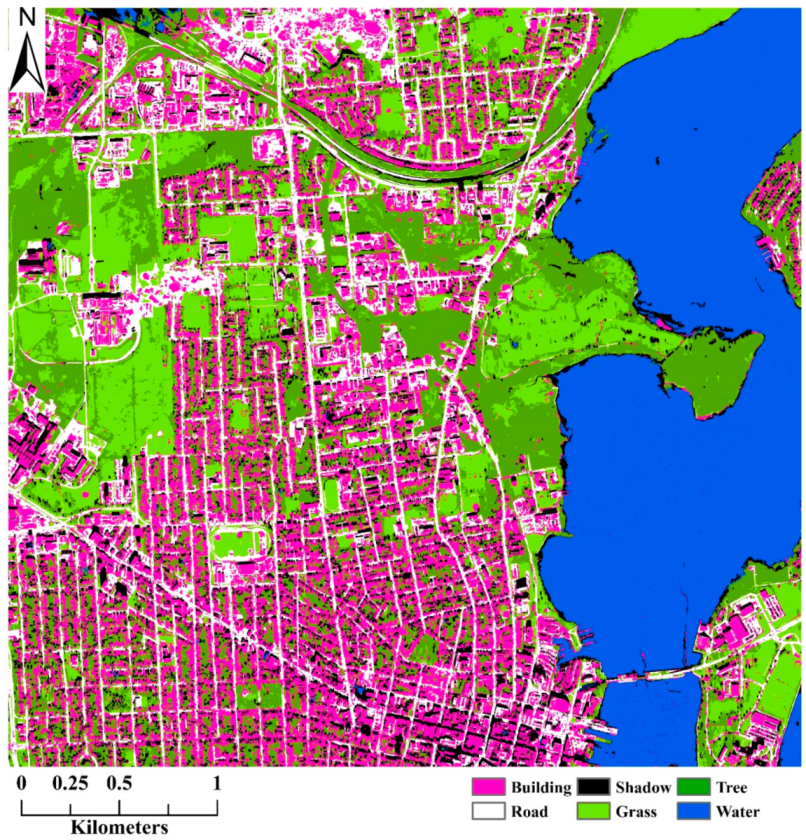
3.1. Study Area and Data

To compare the classifiers in this study, we selected two HSR images. The first image was an aerial HSR image of an urban area in Calhoun, Illinois, USA (Figure 1). This image had a spatial resolution of 30 cm and a radiometric resolution of 8 bits with four spectral channels (i.e., Red, Green, Blue, and NIR). This HSR image is freely accessible through EarthExplorer. The urban area covered in this image consists of heterogeneous and diverse LULC features, making it suitable for our analyses.
The other image used was a WorldView-2 image acquired in 2010 covering the city of Kingston, Ontario, Canada (Figure 2). For this study, we used the RGB and NIR-1 bands. We also pansharpened the image to take advantage of the 50 cm spatial resolution provided by the panchromatic band. As in the first image, various complex urban LULCs were present in this image. However, this image had a more heterogeneous structure than the other image did, which was useful to challenge different classifiers utilized.

3.2. Image Segmentation and Feature Extraction

In this study, we used the multiresolution segmentation (MRS) algorithm proposed by Baatz and Schäpe [45], which is one of the most commonly used segmentation algorithms for RS image analysis. The MRS algorithm has three free parameters: scale parameter (SP), color/shape weights, and smoothness/compactness weights. The SP is the most important parameter because it implicitly governs the average size of image segments, and setting it appropriately is critical for achieving accurate segmentation and classification results [46,47,48]. This parameter is conventionally set through a time-consuming and subjective trial-and-error process. To overcome this problem, automatic approaches are widely used to generate optimal segmentation results. In several studies, it has been emphasized that different LULCs have their own inherent scales [6,28,49]. It is therefore often better to segment an image using multiple SPs rather than a universal one to extract different LULCs of interest [46]. In this regard, to extract buildings using the MRS algorithm, we segmented the image using the SP derived from the degree-2 polynomial (DP) model proposed by Jozdani, et al. [6]. The polynomial model is only applicable for buildings, so for the remaining classes, we employed Estimation of Scale Parameter (ESP) tool [5,28] (one of the most commonly used automatic approaches to the estimation of SP). However, for the 50 cm image, the SP estimated by the ESP was very coarse and did not lead to an acceptable segmentation. We instead estimated an appropriate SP for the other classes using the supervised method F-measure [46].
To take advantage of the multiscale power of GEOBIA, the two segmentation levels were then overlaid, and the spectral/spatial/texture features computed for the coarser level (i.e., the superobjects) were assigned to the segments they contained in the finer segmentation level (i.e., the subobjects). Utilizing this type of multiscale approach was found to improve classification accuracy in past GEOBIA studies utilizing ML classifiers [3,50,51].
We aimed to use a high-dimensional data set in our experiments because one of the main goals of this study was to evaluate the potential of each model to handle high-dimensional data, and to analyze the performance and efficacy of autoencoder models in comparison with the other models for urban LULC mapping. For this purpose, in addition to the features recommended Ma, et al. [51], we calculated some other useful features for the image segments generated. The features calculated were as follows (overall, 33 features).
  • Spectral features: “brightness”, “mean”, “standard deviation”, “skewness”.
  • Spatial features: “area”, “asymmetry”, “border index”, “border length”, “compactness”, “main direction”, “roundness”, “shape index”, “length”.
  • Textural features: “GLCM” features (homogeneity, contrast, dissimilarity, entropy, Ang. 2nd moment, mean, standard deviation, correlation).
  • Vegetation index: “NDVI”.
Each of the computed features was then standardized (to have a mean of 0 and a standard deviation of 1).
In recent years, there have been a few studies on the integration of GEOBIA and CNN [17,25,27,29]. In this study, we integrated a 50-layer ResNet model [52] with the image segments generated by MRS. In this approach, the first step was to prepare the inputs (image patches) that should be fed into the network. The size of the image patches in this CNN model is 224 × 224 with three channels, although data sets having more channels can be used through a simple modification of the model. To incorporate GEOBIA into CNN, we followed a similar approach proposed by Fu, et al. [17] and Zhang, et al. [27] to first extract image patches corresponding to the image objects generated by the segmentation. In this approach, we computed the smallest oriented bounding box (with minimum areas) of each image segment. Then, we extracted the bounding boxes enclosing image segments, and resized them to 224 × 224. Finally, to keep the aspect ratio fixed, we used zero padding while resizing the image patches. The final image patches therefore had a size of 224 × 224 with four channels (RGB and NIR). When integrating CNN and GEOBIA, the segments themselves are not generally extracted and resized to be directly used as inputs into a CNN because it eliminates the context information, and thus affecting the performance of the CNN to extract concrete features. There are generally two ways of taking advantage of CNNs (and generally DNNs); the first way is to use a pretrained model that can be retrained on a new data set. The other way is to train the model from scratch. The advantage of the first approach is that the model can be trained and could lead to satisfying results even if a limited number of data are used. This approach known as transfer learning, however, requires using the same size and number of channels (i.e., in most cases, only RGB) for the new data set. Since we intended to use four channels, we chose the second approach and trained the model from scratch.
In this study, from the 30 cm image, we gathered statistically independent and nonadjacent LULC training and testing data (training/testing segments) using a simple random sampling (SRS) approach to make sure the analyses and results are not biased [53]. Overall, 5571 image segments, representing six different LULC types (buildings (1559 samples), road (908 samples), trees (1181 samples), grass (1084 samples), water (107 samples), shadow (732)), were collected for the training set, and 1248 pixels for the testing set to evaluate the performance of the classification models established. From the 50 cm image, 1030 samples for buildings, 764 samples for road, 352 samples for shadow, 684 samples for grass, 415 samples for trees, and 355 samples for water were extracted. A total of 1432 pixels were also randomly selected as the test set for this image. It should be also noted that no training/test samples from the cloud-contaminated parts of the 50 cm image were collected, because the underlying LULC types were not apparent in those areas. Since the training data gathered for both the images were imbalanced, we applied the Synthetic Minority Oversampling Technique (SMOTE) [54] to artificially balance the training set, as this was found beneficial in past studies using imbalanced data [55,56] and machine learning classifiers [57].

3.3. Implementation of Classifiers

We implemented all the classification models in this study using Python programming language. To implement the DL classifiers, we used the “TensorFlow” framework which is an open source library developed by “Google Brain” [58]. TensorFlow allows the implementation of a DL network on either CPU or GPU, provided that the GPU is supported by the framework. In this study, we implemented the networks on an Nvidia GeForce GTX 1080 Ti GPU. It is generally recommended to implement DNNs on a supported powerful GPU because it significantly reduces the execution time during training and inference. The RF, GB, BT, and SVM classifiers were applied using the open source “scikit-learn” module [59], which is the most commonly used ML module in Python. For the XGB classifier, we applied the “XGBoost” module in Python. As a trade-off between fast convergence and less execution time, a learning rate of 0.1 was chosen for the XGB and GB models. The hyperparameters of the SVM model were selected using a 5-fold cross-validation (C = 100, ε = 0.01).
As already stated, autoencoders are unsupervised ML algorithms that are typically used as a pretraining step. Therefore, for supervised classification, they should be combined with a supervised classifier. In other words, the supervised classifier applies the features generated by the autoencoder to perform classification. In this study, after training the autoencoder models, we used their lower-level layers in an MLP model to establish a new classifier using these pretrained layers. We also performed fine-tuning to the model through applying back-propagation algorithm to the encoder layers.
When training a neural network model, choosing a stopping criterion is important because it helps preclude overfitting, especially when (very) deep networks are utilized. One of the most commonly used stopping criteria is to terminate training process after a certain number of iterations. In this study, we trained the autoencoder models for 200 iterations and then recorded their encoder layers for supervised classification. The MLP and CNN models were trained for 2000, and 300 iterations, respectively. For all the DL models, we used Adam optimizer to minimize the loss function, a learning rate of 0.001 in the optimization process, and Rectified Linear Unit (ReLU) as the activation function. For the MLP and all the autoencoders in the supervised setup, we applied the l2 regularizer and a dropout of 0.25 to reduce overfitting during classification. For the SAE model, the sparsity parameter and the sparsity weight were both set to 0.1. The remaining parameter settings of the four neural networks applied are presented in Table 1.

4. Results and Discussion

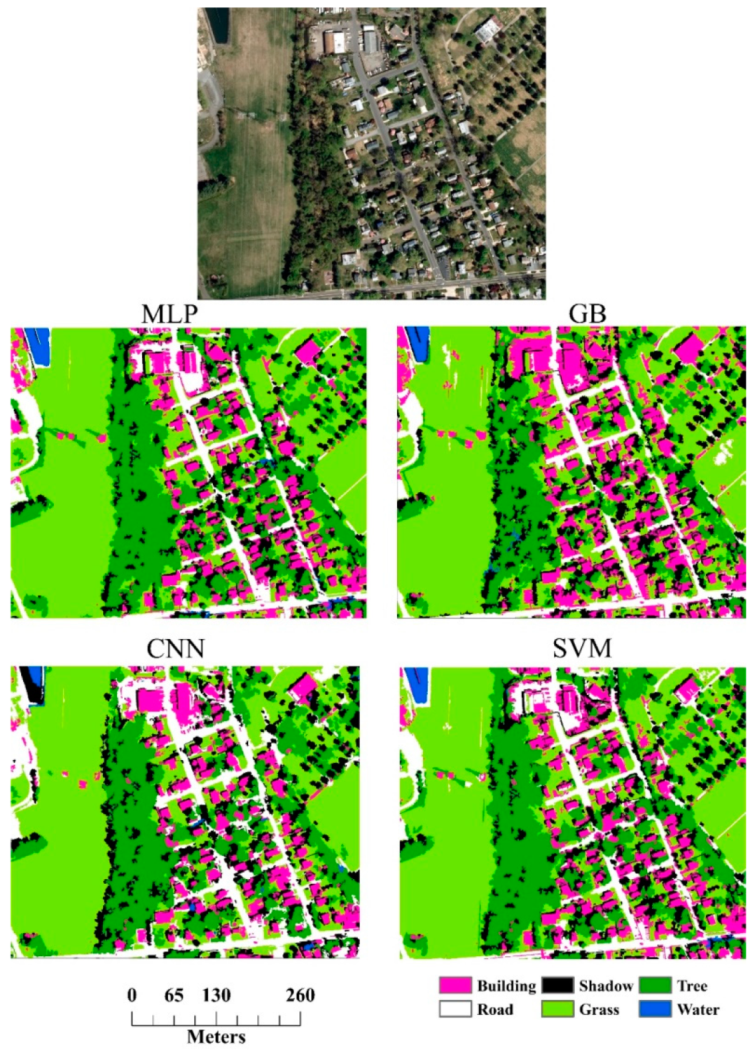
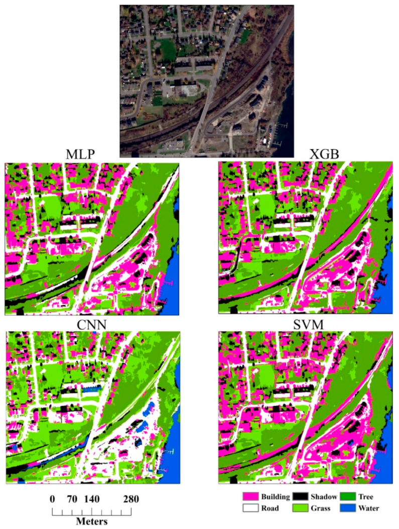
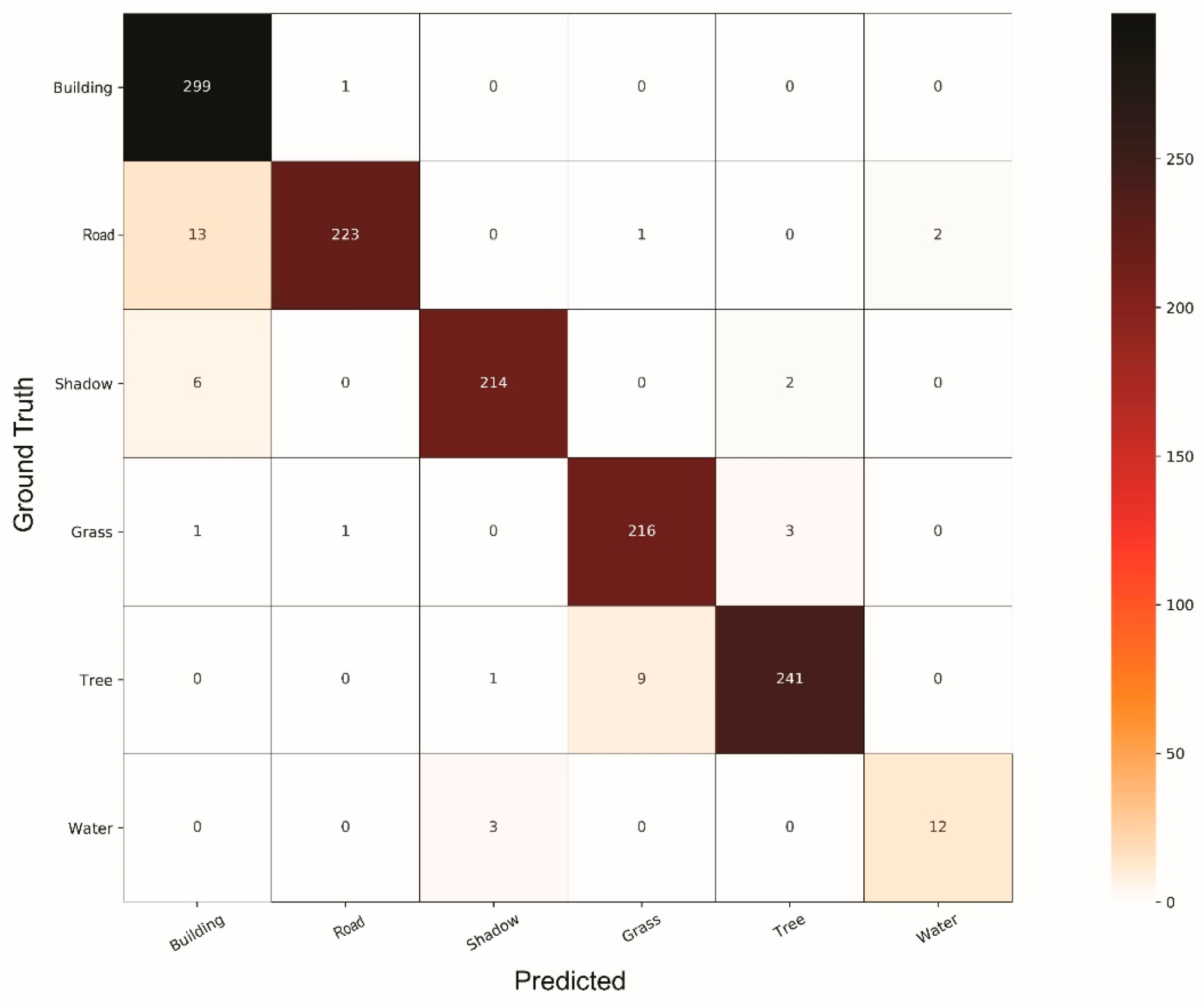
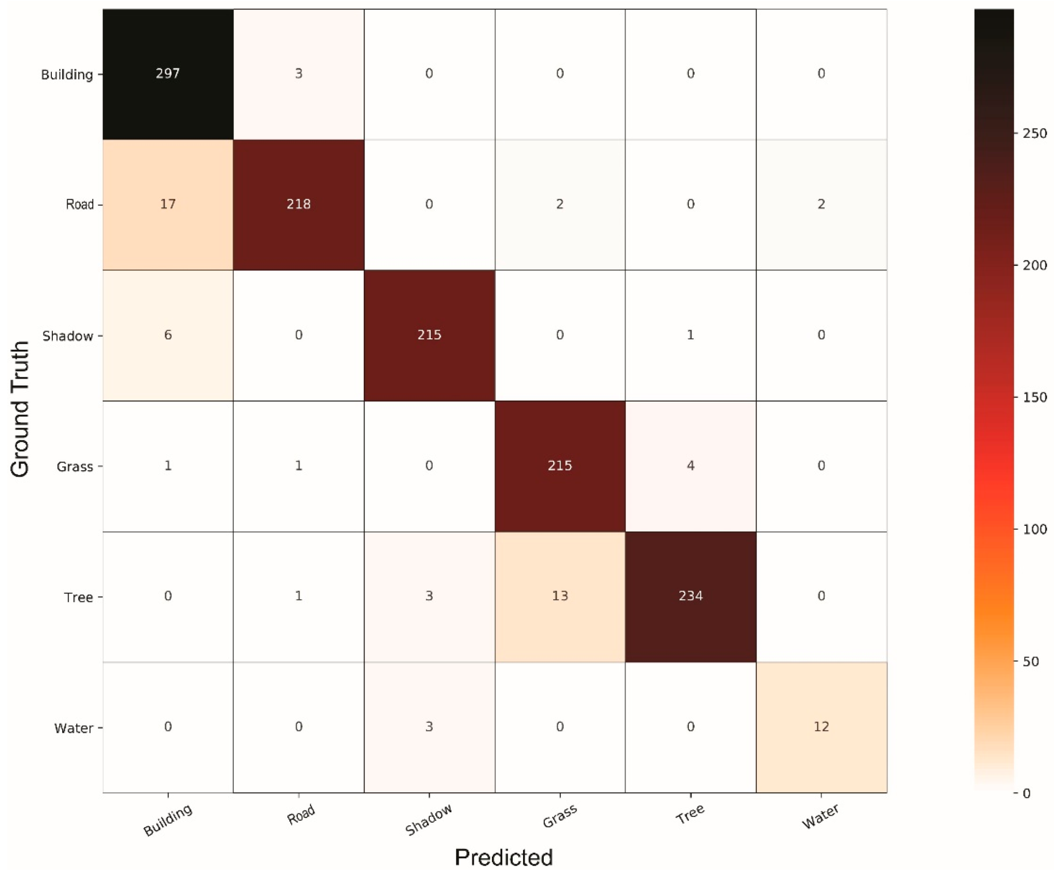
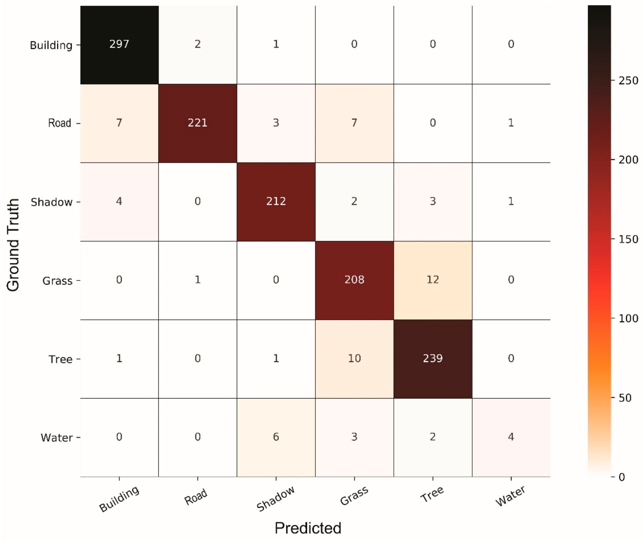
4.1. Comparison of Classifiers

Based on Table 2, the best accuracies were achieved by the MLP model for the 30 cm image. The other DNNs led to > 2% worse accuracy than the MLP. Of the ensemble classifiers, the BT (the simplest ensemble classifier tested) achieved the worst overall accuracy, and this can likely be ascribed to the fact that it was unable to handle the high dimensionality of the data. As elaborated earlier, BT uses the entire feature set for training the DTs in the ensemble. Thus, when features are highly correlated, the corresponding individual DTs are also highly correlated, and the BT model suffers from overfitting [26]. The RF model reduces the correlation between the DTs in the ensemble through random sampling of features, which led to an increase in classification accuracy in our experiment. The GB and XGB models led to further improvement in classification accuracy in our experiments. From this, it can be shown that even using tree stumps as a base classifier GB can generate accurate results because the ensemble is composed in such a way that each tree generated is an improved version of the previous one. Although XGB performed slightly worse than GB, it is much faster thanks to its highly parallelized implementation/concept. This advantage is specifically valuable when working with very large data sets (e.g., classification of time series RS images). As the data set become larger, it can also be speculated that XGB starts performing better than GB in terms of accuracy due to its regulation term that helps increase the generalizability of the algorithm.
To realize if the difference between the XGB and GB classifiers was statistically significant, we applied a McNemar’s test. The null hypothesis of this test is that there is no difference between the two results. Applying this test led to a large p-value (> 0.05) indicating that the two classifiers were not statistically different from each other. After these two classifiers, the SVM model was the most accurate one, with a small difference from the XGB.
Of the models applied, the SAE model had the worst performance. This shows that applying pretraining in a GEOBIA setup could not result in any accuracy improvement, though a high dimensional data set was applied. In fact, squeezing the feature space did not add any useful information to the classification construct to obtain a more accurate result in the 30 cm image.
In Appendix B (Figure A4, Figure A5, Figure A6 and Figure A7), the confusion matrices for the MLP, GB, SVM, and CNN classification results (i.e., the most accurate classifiers from each category in our study) can be seen. From these confusion matrices, the greatest difficulty for all the models was differentiating between grass and tree. This was mainly due to the high degree of spectral similarity between some of the samples in the two LULC classes. Moreover, none of the spatial and/or textural features computed were capable of significantly differentiating between them. Another common source of classification error was the spectral similarity between the building and road classes. Buildings in particular were highly heterogeneous in terms of their spectral and structural (spatial) properties, and mapping them is perhaps one of the most challenging parts in urban classification using RS. One of the greatest virtues of the MLP applied was its higher accuracy in the classification of building samples. As our results showed, the smallest number of misclassified building samples was obtained by the MLP model.
Besides providing the entire map generated by MLP (as the most accurate classifier for this 30 cm image) in Appendix C (Figure A12), a subset of the classification map generated by each of the MLP, GB, SVM, and CNN models for visual comparison is illustrated in Figure 3.
According to Table 3, the experiments on the 50 cm image led to similar conclusions. The MLP classifier again produced the most accurate result. In contrast to the 30 cm image, the XGB model resulted in a slightly better result than the GB. Again, this difference was not statistically significant. Of the ensemble classifiers, the BT model led to the worst accuracies. This, however, should be noted that the accuracy difference between this classifier and the other ensemble ones was more significant than the one generated for the 30 cm image.
As with the previous results for the 30 cm image, the CNN model failed to produce more accurate results than the other DL models did. According to these experiments, although it was hypothesized that integrating a CNN model and GEOBIA could better help model object boundaries; this integration was highly dependent on the object’s shape and size. If the object is elongated, the bounding box enclosing it may largely contain other LULC types. Or if the segment is very small, the model may not be able to extract and learn useful features. These two problems are exacerbated when it comes to extremely resizing image patches (i.e., bounding boxes which are either very small or very large) to correspond the input size of the network. This therefore misleads the classifier which causes a high rate of misclassification.
The confusion matrices (Figure A8, Figure A9, Figure A10 and Figure A11) computed for the four classifiers on the 50 cm image echoed the same problem of the classifiers with the building and road and grass and tree classes. In addition to this problem, the results of this image showed that some samples of the shadow and building classes were misclassified. This misclassification was generally caused by the fact that some shadow samples in both the training and test sets were not pure and/or were composed of some parts of the buildings. In other words, the texture of some shadow samples was not very homogeneous to be correctly classified. As a result, the classifiers failed to correctly classify some of the samples of these two classes to their true ones.
Besides providing the entire map generated by MLP (as the most accurate classifier for this 50 cm image) in Figure A13, a subset of the 50 cm image along with the generated maps by MLP, XGB, CNN, and SVM classifiers is illustrated in Figure 4.
As the classification maps produced for the 50 cm image depict, the CNN resulted in the noisiest result, though it produced a more homogenous map for the 30 cm image. Another important strength of the MLP in the 50 cm image was correctly classifying elongated features, especially roads. According to Figure 4, the MLP classified roads much more accurate than the other classifiers.

4.2. General Discussion

Although our experiments showed the superiority of MLP over the other state-of-the-art ML classifiers in terms of classification accuracy, there are some important considerations regarding its efficiency that need to be further discussed. In general, DL models tend to be more complex than ensemble models and SVM. This means that they need more parameter tuning in the training stage. As stated earlier, parameter tuning and optimization are often performed using cross-validation for ML algorithms. However, in some cases, DL models could have millions of weights to be optimized in each iteration [42]. Therefore, training such models is itself time consuming, and thus manual tuning or rules of thumb are preferred over cross-validation, which could potentially have a negative impact on the accuracy of the network. An obvious solution is to implement the entire model on a GPU to significantly decrease training time. This, as a result, allows the user to test different parameter settings that better meet the requirements of the application for which the DL model is to be used. Another popular strategy is to take advantage of transfer learning [60]. In this respect, instead of training a model from scratch, pretrained models are retrained on the user’s classes of interest. Transfer learning has two important advantages: (1) it does not typically need many new training data and (2) the weights of the model can be optimized on the new data set in a much fewer number of iterations. Novelli, et al. [61] conducted an experiment to analyze two main scenarios (i.e., fine-tuning the model and using the pretrained model as a feature extractor) for retraining a pretrained model. In that study, it was shown that fine-tuning of pretrained models led to better accuracy. The deep models that are widely used in the literature, however, may not always be useful to be generalized to all domains. For example, they may not have been designed to accept inputs with more than three channels (i.e., RGB), which may not be favorable for RS applications where images usually have extra channels [17]. Therefore, these models should be redesigned and trained from scratch, which is computationally inefficient and needs sufficient training data [61].
Moreover, DNNs is that their performance depends greatly on the number of labeled training samples; that is, DNNs generally perform better if they are fed with a large number of labeled samples [25]. In many RS applications, collecting a large number of labeled samples for each class of interest is difficult and error prone. For example, over some urban areas, there might not be a sufficient number of water bodies or green spaces to use for training the model. Moreover, in some cases, the complexity of the urban landscape may require the analyst to conduct field surveys to gather ground truth data, which is costly and time consuming. Considering the above-mentioned factors, it may still be more efficient to use non-DL algorithms, especially GB/XGB and SVM that can perform well even using limited training samples, for urban mapping within a GEOBIA framework, which have been widely reported to be very accurate [19,26].
Aside from selecting a good classifier, the features extracted from the image are also of importance. In a traditional GEOBIA approach, the analyst needs to use hand-crafted features in the classification phase. Undoubtedly, the number and the choice of the features both affect the final classification accuracy. Despite few studies on appropriate image (object) features for LULC mapping (like [51]), the previously recommended features could be highly domain specific, and could not be properly generalized to other LULC types and study areas. In contrast to hand-engineered features, the features in a CNN are learned automatically from the input data during training. These distinctive, machine-learned features are learned by the CNN based on classes spectral, contextual, and spatial properties, and thus increasing their generalizability capabilities.

5. Conclusions

In this paper, we evaluated the potential of several object-based DL models (i.e., MLP, RAE, SAE, VAE, and CNN) in comparison with other state-of-the-art ML classifiers (i.e., SVM, RF, BT, GB, and XGB) for object-based urban LULC mapping over a complex landscape. We applied our experiments on two HSR RS images (one of which an aerial image with 30 cm resolution, and the other a pansharpened WorldView-2 image with 50 cm resolution). As the experiments indicated, MLP model led to the most accurate classification results. However, it is also important to note that GB/XGB and SVM produced highly accurate classification results as well, demonstrating the versatility of these ML algorithms. This should be highlighted that while there is hype towards DL, other ML classifiers may still produce very close results to those of DNNs. This is particularly important because the complexity of tuning a DNNs can be time consuming and sometimes confusing, so simpler classifiers like SVM may be preferable in some cases (e.g., when training data is sparse).
In this study, one of our hypotheses was that the use of autoencoders as pretraining procedure would improve the classification results. Although autoencoders are often reported to be useful as a proxy for addressing the limited number of training data, our experiments showed that the use of autoencoders for unsupervised pretraining not only did not improve the supervised classification accuracy, but also degraded the accuracy. In fact, applying an MLP alone without any pretraining resulted in more accurate results.
The McNemar’s test also showed that the XGB and GB and RAE and SAE classifiers trained for the 30 cm image were not statistically different from each other, respectively. For the 50 cm image, the McNemar’s test indicated that the XGB and GB; SVM and RAE; and SAE and RF classifiers were not statistically different, respectively.
The last lesson drawn from this study was that integration of CNN with GEOBIA is not yet mature enough. According to the experiments in this study, we found that this integration did not add any improvement to the classification of the two images applied, and thus led to lower accuracies than the other DNNs employed. This as a result demands for more in-depth research in the future on the ways these two approaches can more optimally take advantage of each other’s strengths for supervised classification of RS images.

Author Contributions

S.E.J conceptualized the methodology, performed the analyses, and wrote the manuscript with B.A.J., D.C supervised the research and improved the methodology and analyses, and edited the final manuscript.

Funding

This research was funded by Natural Sciences and Engineering Research Council of Canada (NSERC) grant number RGPIN-2019-05773 awarded to D.C.

Conflicts of Interest

The authors declare no conflicts of interest.

Appendix A

Schematic structures of MLP and autoencoders can be seen in this appendix.
Figure A1. Graphical representation of an MLP model with two hidden layers.
Remotesensing 11 01713 g0a1
Figure A2. Graphical representation of a regular autoencoder model with a hidden layer.
Remotesensing 11 01713 g0a2
Figure A3. Graphical representation of an SAE model with three hidden layers. Note: Gray-colored circles are neurons deactivated using the regularization term.
Remotesensing 11 01713 g0a3

Appendix B

The confusion matrices calculated for the classifiers trained on the 30 cm and 50 cm test images
Figure A4. Confusion matrix derived from the MLP model for 30 cm image.
Remotesensing 11 01713 g0a4
Figure A5. Confusion matrix derived from the GB model for 30 cm image.
Remotesensing 11 01713 g0a5
Figure A6. Confusion matrix of the SVM for 30 cm image.
Remotesensing 11 01713 g0a6
Figure A7. Confusion matrix of the CNN model for 30 cm image.
Remotesensing 11 01713 g0a7
Figure A8. Confusion matrix of the MLP model for 50 cm image.
Remotesensing 11 01713 g0a8
Figure A9. Confusion matrix of the XGB model for 50 cm image.
Remotesensing 11 01713 g0a9
Figure A10. Confusion matrix of the SVM model for 50 cm image.
Remotesensing 11 01713 g0a10
Figure A11. Confusion matrix of the CNN model for 50 cm image.
Remotesensing 11 01713 g0a11

Appendix C

The final classification maps produced by the most accurate classifiers (MLPs) for the 30 cm and 50 cm images, respectively.
Figure A12. Classification map generated by combining classification maps of the MLP model for the 30 cm image.
Remotesensing 11 01713 g0a12
Figure A13. Classification map generated by combining classification maps of the MLP model for the 50 cm image.
Remotesensing 11 01713 g0a13

References

  1. Blaschke, T. Object based image analysis for remote sensing. ISPRS J. Photogramm. Remote Sens. 2010, 65, 2–16. [Google Scholar] [CrossRef] [Green Version]
  2. Myint, S.W.; Gober, P.; Brazel, A.; Grossman-Clarke, S.; Weng, Q. Per-pixel vs. object-based classification of urban land cover extraction using high spatial resolution imagery. Remote Sens. Environ. 2011, 115, 1145–1161. [Google Scholar] [CrossRef]
  3. Johnson, B.; Xie, Z. Classifying a high resolution image of an urban area using super-object information. ISPRS J. Photogramm. Remote Sens. 2013, 83, 40–49. [Google Scholar] [CrossRef]
  4. Blaschke, T.; Hay, G.J.; Kelly, M.; Lang, S.; Hofmann, P.; Addink, E.; Queiroz Feitosa, R.; van der Meer, F.; van der Werff, H.; van Coillie, F.; et al. Geographic Object-Based Image Analysis—Towards a new paradigm. ISPRS J. Photogramm. Remote Sens. 2014, 87, 180–191. [Google Scholar] [CrossRef] [PubMed]
  5. Drǎguţ, L.; Tiede, D.; Levick, S.R. ESP: A tool to estimate scale parameter for multiresolution image segmentation of remotely sensed data. Int. J. Geogr. Inf. Sci. 2010, 24, 859–871. [Google Scholar] [CrossRef]
  6. Jozdani, S.E.; Momeni, M.; Johnson, B.A.; Sattari, M. A regression modelling approach for optimizing segmentation scale parameters to extract buildings of different sizes. Int. J. Remote Sens. 2018, 39, 684–703. [Google Scholar] [CrossRef]
  7. Yu, L.; Liang, L.; Wang, J.; Zhao, Y.; Cheng, Q.; Hu, L.; Liu, S.; Yu, L.; Wang, X.; Zhu, P.; et al. Meta-discoveries from a synthesis of satellite-based land-cover mapping research. Int. J. Remote Sens. 2014, 35, 4573–4588. [Google Scholar] [CrossRef]
  8. Dietterich, T.G. An Experimental Comparison of Three Methods for Constructing Ensembles of Decision Trees: Bagging, Boosting, and Randomization. Mach. Learn. 2000, 40, 139–157. [Google Scholar] [CrossRef]
  9. Breiman, L. Random Forests. Mach. Learn. 2001, 45, 5–32. [Google Scholar] [CrossRef] [Green Version]
  10. Cortes, C.; Vapnik, V. Support-vector networks. Mach. Learn. 1995, 20, 273–297. [Google Scholar] [CrossRef]
  11. Ma, L.; Li, M.; Ma, X.; Cheng, L.; Du, P.; Liu, Y. A review of supervised object-based land-cover image classification. ISPRS J. Photogramm. Remote Sens. 2017, 130, 277–293. [Google Scholar] [CrossRef]
  12. Hinton, G.E.; Osindero, S.; Teh, Y.-W. A fast learning algorithm for deep belief nets. Neural Comput. 2006, 18, 1527–1554. [Google Scholar] [CrossRef] [PubMed]
  13. Zhu, X.X.; Tuia, D.; Mou, L.; Xia, G.; Zhang, L.; Xu, F.; Fraundorfer, F. Deep Learning in Remote Sensing: A Comprehensive Review and List of Resources. IEEE Geosci. Remote Sens. Mag. 2017, 5, 8–36. [Google Scholar] [CrossRef] [Green Version]
  14. Boualleg, Y.; Farah, M.; Farah, I.R. Remote Sensing Scene Classification Using Convolutional Features and Deep Forest Classifier. IEEE Geosci. Remote Sens. Lett. 2019, 1–5. [Google Scholar] [CrossRef]
  15. Lv, X.; Ming, D.; Chen, Y.; Wang, M. Very high resolution remote sensing image classification with SEEDS-CNN and scale effect analysis for superpixel CNN classification. Int. J. Remote Sens. 2019, 40, 506–531. [Google Scholar] [CrossRef]
  16. Zhao, J.; Yu, L.; Xu, Y.; Ren, H.; Huang, X.; Gong, P. Exploring the addition of Landsat 8 thermal band in land-cover mapping. Int. J. Remote Sens. 2019, 40, 4544–4559. [Google Scholar] [CrossRef]
  17. Fu, T.; Ma, L.; Li, M.; Johnson, B.A. Using convolutional neural network to identify irregular segmentation objects from very high-resolution remote sensing imagery. J. Appl. Remote Sens. 2018, 12, 21. [Google Scholar] [CrossRef]
  18. Liu, S.; Qi, Z.; Li, X.; Yeh, G.A. Integration of Convolutional Neural Networks and Object-Based Post-Classification Refinement for Land Use and Land Cover Mapping with Optical and SAR Data. Remote Sens. 2019, 11, 690. [Google Scholar] [CrossRef]
  19. Liu, P.; Choo, K.-K.R.; Wang, L.; Huang, F. SVM or deep learning? A comparative study on remote sensing image classification. Soft Comput. 2017, 21, 7053–7065. [Google Scholar] [CrossRef]
  20. Ng, A. Sparse Autoencoder. 2010. Available online: https://web.Stanf.Edu/Cl./Cs294a/Sparseautoencoder.pdf (accessed on 10 August 2017).
  21. Zhang, X.; Chen, G.; Wang, W.; Wang, Q.; Dai, F. Object-Based Land-Cover Supervised Classification for Very-High-Resolution UAV Images Using Stacked Denoising Autoencoders. IEEE J. Sel. Top. Appl. Earth Obs. Remote Sens. 2017, 10, 3373–3385. [Google Scholar] [CrossRef]
  22. Vincent, P.; Larochelle, H.; Lajoie, I.; Bengio, Y.; Manzagol, P.-A. Stacked Denoising Autoencoders: Learning Useful Representations in a Deep Network with a Local Denoising Criterion. J. Mach. Learn. Res. 2010, 11, 3371–3408. [Google Scholar]
  23. Liu, T.; Abd-Elrahman, A. Deep convolutional neural network training enrichment using multi-view object-based analysis of Unmanned Aerial systems imagery for wetlands classification. ISPRS J. Photogramm. Remote Sens. 2018, 139, 154–170. [Google Scholar] [CrossRef]
  24. Belgiu, M.; Drăguţ, L. Random forest in remote sensing: A review of applications and future directions. ISPRS J. Photogramm. Remote Sens. 2016, 114, 24–31. [Google Scholar] [CrossRef]
  25. Liu, T.; Abd-Elrahman, A.; Morton, J.; Wilhelm, V.L. Comparing fully convolutional networks, random forest, support vector machine, and patch-based deep convolutional neural networks for object-based wetland mapping using images from small unmanned aircraft system. GIScience Remote Sens. 2018, 55, 243–264. [Google Scholar] [CrossRef]
  26. Maxwell, A.E.; Warner, T.A.; Fang, F. Implementation of machine-learning classification in remote sensing: An applied review. Int. J. Remote Sens. 2018, 39, 2784–2817. [Google Scholar] [CrossRef]
  27. Zhang, X.; Wang, Q.; Chen, G.; Dai, F.; Zhu, K.; Gong, Y.; Xie, Y. An object-based supervised classification framework for very-high-resolution remote sensing images using convolutional neural networks. Remote Sens. Lett. 2018, 9, 373–382. [Google Scholar] [CrossRef]
  28. Drăguţ, L.; Csillik, O.; Eisank, C.; Tiede, D. Automated parameterisation for multi-scale image segmentation on multiple layers. ISPRS J. Photogramm. Remote Sens. 2014, 88, 119–127. [Google Scholar] [CrossRef]
  29. Zhang, C.; Sargent, I.; Pan, X.; Li, H.; Gardiner, A.; Hare, J.; Atkinson, P.M. An object-based convolutional neural network (OCNN) for urban land use classification. Remote Sens. Environ. 2018, 216, 57–70. [Google Scholar] [CrossRef] [Green Version]
  30. Mason, L.; Baxter, J.; Bartlett, P.; Frean, M. Boosting algorithms as gradient descent. In Proceedings of the 12th International Conference on Neural Information, Denver, CO, USA, 29 November–4 December 1999. [Google Scholar]
  31. Chen, T.; Guestrin, C. XGBoost: Reliable Large-scale Tree Boosting System. arXiv 2016. [Google Scholar] [CrossRef]
  32. Breiman, L. Classification and Regression Trees; Wadsworth Statistics Series; Chapman and Hall: London, UK, 1984; Volume 19, p. 368. [Google Scholar]
  33. Breiman, L. Bagging Predictors. Mach. Learn. 1996, 24, 123–140. [Google Scholar] [CrossRef]
  34. Lawrence, R.L.; Wood, S.D.; Sheley, R.L. Mapping invasive plants using hyperspectral imagery and Breiman Cutler classifications (randomForest). Remote Sens. Environ. 2006, 100, 356–362. [Google Scholar] [CrossRef]
  35. Freund, Y.; Schapire, R.E. A Decision-Theoretic Generalization of On-Line Learning and an Application to Boosting. J. Comput. Syst. Sci. 1997, 55, 119–139. [Google Scholar] [CrossRef] [Green Version]
  36. Friedman, J.H. Greedy function approximation: A gradient boosting machine. Ann. Stat. 2001, 29, 1189–1232. [Google Scholar] [CrossRef]
  37. Georganos, S.; Grippa, T.; Vanhuysse, S.; Lennert, M.; Shimoni, M.; Kalogirou, S.; Wolff, E. Less is more: Optimizing classification performance through feature selection in a very-high-resolution remote sensing object-based urban application. GIScience Remote Sens. 2018, 55, 221–242. [Google Scholar] [CrossRef]
  38. Georganos, S.; Grippa, T.; Vanhuysse, S.; Lennert, M.; Shimoni, M.; Wolff, E. Very High Resolution Object-Based Land Use–Land Cover Urban Classification Using Extreme Gradient Boosting. IEEE Geosci. Remote Sens. Lett. 2018, 15, 607–611. [Google Scholar] [CrossRef]
  39. Melgani, F.; Bruzzone, L. Classification of hyperspectral remote sensing images with support vector machines. IEEE Trans. Geosci. Remote Sens. 2004, 42, 1778–1790. [Google Scholar] [CrossRef] [Green Version]
  40. Mountrakis, G.; Im, J.; Ogole, C. Support vector machines in remote sensing: A review. ISPRS J. Photogramm. Remote Sens. 2011, 66, 247–259. [Google Scholar] [CrossRef]
  41. Glorot, X.; Bengio, Y. Understanding the difficulty of training deep feedforward neural networks. In Proceedings of the Thirteenth International Conference on Artificial Intelligence and Statistics, Sardinia, Italy, 13–15 May 2010; pp. 249–256. [Google Scholar]
  42. LeCun, Y.; Bengio, Y.; Hinton, G. Deep learning. Nature 2015, 521, 436. [Google Scholar] [CrossRef]
  43. Kingma, D.P.; Welling, M. Auto-Encoding Variational Bayes. arXiv 2013, arXiv:1312.6114. [Google Scholar]
  44. Doersch, C. Tutorial on Variational Autoencoders. arXiv 2016, arXiv:1606.05908. [Google Scholar]
  45. Baatz, M.; Schäpe, A. Multiresolution Segmentation: An optimization approach for high quality multi-scale image segmentation. In Angewandte Geographische Informationsverarbeitung XII. Beiträge zum AGIT-Symposium Salzburg 2000; Herbert Wichmann Verlag: Karlsruhe, Germany, 2000; pp. 12–23. [Google Scholar]
  46. Johnson, A.B.; Bragais, M.; Endo, I.; Magcale-Macandog, B.D.; Macandog, B.P. Image Segmentation Parameter Optimization Considering Within- and Between-Segment Heterogeneity at Multiple Scale Levels: Test Case for Mapping Residential Areas Using Landsat Imagery. ISPRS Int. J. Geo-Inf. 2015, 4, 2292–2305. [Google Scholar] [CrossRef] [Green Version]
  47. Grybas, H.; Melendy, L.; Congalton, R.G. A comparison of unsupervised segmentation parameter optimization approaches using moderate- and high-resolution imagery. GIScience Remote Sens. 2017, 54, 515–533. [Google Scholar] [CrossRef]
  48. Georganos, S.; Lennert, M.; Grippa, T.; Vanhuysse, S.; Johnson, B.; Wolff, E. Normalization in Unsupervised Segmentation Parameter Optimization: A Solution Based on Local Regression Trend Analysis. Remote Sens. 2018, 10, 222. [Google Scholar] [CrossRef]
  49. Johnson, A.B.; Jozdani, E.S. Identifying Generalizable Image Segmentation Parameters for Urban Land Cover Mapping through Meta-Analysis and Regression Tree Modeling. Remote Sens. 2018, 10, 73. [Google Scholar] [CrossRef]
  50. Gholoobi, M.; Kumar, L. Using object-based hierarchical classification to extract land use land cover classes from high-resolution satellite imagery in a complex urban area. J. Appl. Remote Sens. 2015, 9. [Google Scholar] [CrossRef]
  51. Ma, L.; Cheng, L.; Li, M.; Liu, Y.; Ma, X. Training set size, scale, and features in Geographic Object-Based Image Analysis of very high resolution unmanned aerial vehicle imagery. ISPRS J. Photogramm. Remote Sens. 2015, 102, 14–27. [Google Scholar] [CrossRef]
  52. He, K.; Zhang, X.; Ren, S.; Sun, J. Deep Residual Learning for Image Recognition. In Proceedings of the 2016 IEEE Conference on Computer Vision and Pattern Recognition (CVPR), Las Vegas, NV, USA, 27–30 June 2016; pp. 770–778. [Google Scholar]
  53. Johnson, A.B. Scale Issues Related to the Accuracy Assessment of Land Use/Land Cover Maps Produced Using Multi-Resolution Data: Comments on “The Improvement of Land Cover Classification by Thermal Remote Sensing”. Remote Sens. 2015, 7, 8368–8390. [Google Scholar] [CrossRef]
  54. Chawla, N.V.; Bowyer, K.W.; Hall, L.O.; Kegelmeyer, W.P. SMOTE: Synthetic minority over-sampling technique. J. Artif. Intell. Res. 2002, 16. [Google Scholar] [CrossRef]
  55. Bogner, C.; Seo, B.; Rohner, D.; Reineking, B. Classification of rare land cover types: Distinguishing annual and perennial crops in an agricultural catchment in South Korea. PLoS ONE 2018, 13, e0190476. [Google Scholar] [CrossRef]
  56. Buda, M.; Maki, A.; Mazurowski, M.A. A systematic study of the class imbalance problem in convolutional neural networks. Neural Netw. 2018, 106, 249–259. [Google Scholar] [CrossRef] [Green Version]
  57. Johnson, B.A.; Tateishi, R.; Hoan, N.T. A hybrid pansharpening approach and multiscale object-based image analysis for mapping diseased pine and oak trees. Int. J. Remote Sens. 2013, 34, 6969–6982. [Google Scholar] [CrossRef]
  58. Abadi, M.; Agarwal, A.; Barham, P.; Brevdo, E.; Chen, Z.; Citro, C.; Corrado, G.S.; Davis, A.; Dean, J.; Devin, M.; et al. TensorFlow: Large-Scale Machine Learning on Heterogeneous Distributed Systems. arXiv 2016, arXiv:1603.04467. [Google Scholar]
  59. Pedregosa, F.; Varoquaux, G.; Gramfort, A.; Michel, V.; Thirion, B.; Grisel, O.; Blondel, M.; Prettenhofer, P.; Weiss, R.; Dubourg, V.; et al. Scikit-learn: Machine Learning in Python. J. Mach. Learn. Res. 2011, 12, 2825–2830. [Google Scholar] [CrossRef]
  60. Ma, L.; Liu, Y.; Zhang, X.; Ye, Y.; Yin, G.; Johnson, B.A. Deep learning in remote sensing applications: A meta-analysis and review. ISPRS J. Photogramm. Remote Sens. 2019, 152, 166–177. [Google Scholar] [CrossRef]
  61. Novelli, A.; Aguilar, A.M.; Aguilar, J.F.; Nemmaoui, A.; Tarantino, E. AssesSeg—A Command Line Tool to Quantify Image Segmentation Quality: A Test Carried Out in Southern Spain from Satellite Imagery. Remote Sens. 2017, 9, 40. [Google Scholar] [CrossRef]
Figure 1. 30 cm aerial image covering an urban area in Calhoun, Illinois, USA.
Remotesensing 11 01713 g001
Figure 2. 50 cm WorldView-2 image covering a subregion the city of Kingston, Ontario, Canada.
Remotesensing 11 01713 g002
Figure 3. Subsets of classification maps generated by the regular deep multilayer perceptron (MLP), Gradient Boosting Trees (GB), convolutional neural network (CNN), and support vector machines (SVM) models generated for the 30 cm image.
Remotesensing 11 01713 g003
Figure 4. Subsets of classification maps generated by the MLP, XGB, CNN, and SVM models for the 50 cm image.
Remotesensing 11 01713 g004
Table 1. Layer configurations of deep learning (DL) models applied.
Model# of Hidden Layers# of Neurons in Each Hidden LayerTotal # of Trainable Parameters
MLP3100-100-10034,306
RAE3100-30-10012,863
SAE2100-10016,833
VAE3100-20-1008213
CNN (ResNet)50Refer to He, et al. [52]23,537,728
Table 2. Accuracy measures derived from the models applied on the 30 cm image.
Classifier (30 cm)Overall AccuracyKappaF1-Score
RF94.470.9310.945
GB95.990.9500.960
XGB95.910.9490.959
BT94.310.9290.944
SVM95.430.9430.954
MLP96.550.9570.965
RAE94.390.9300.945
SAE93.670.9210.938
VAE94.310.9290.945
CNN94.630.9300.944
Table 3. Accuracy measures derived from the models applied on the 50 cm image.
Classifier (50 cm)Overall AccuracyKappaF1-Score
RF92.040.9040.921
GB92.870.9140.929
XGB92.940.9150.930
BT90.780.8890.908
SVM92.450.9090.925
MLP93.640.9230.937
RAE92.450.9090.925
SAE91.890.9020.919
VAE92.730.9130.928
CNN91.410.8960.913

